Simplified Weather-Related Building Energy Disaggregation and Change-Point Regression: Heating and Cooling Energy Use Perspective

Abstract

End-use consumption provides more detailed information than total consumption and reveals the mechanism of energy flow through a given building. Specifically, for weather-sensitive energy end-uses, it enables the prioritization and selection of heating and cooling areas requiring investigation and actions. One of the major barriers to acquiring such heating and cooling information for small- and medium-sized buildings or low-income households is the high cost related to submetering and maintenance. The end-use data, especially for heating and cooling end-uses, of such-sized buildings are a national blind spot. In this study, to alleviate this measurement cost problem, two weather-sensitive energy disaggregation methods were examined: the simplified weather-related energy disaggregation (SED) and change-point regression (CPR) methods. The first is a nonparametric approach based on heuristics, whereas the second is a parametric approach. A comparative analysis (one-way ANOVA, correlation analysis, and individual comparison) was performed to explore the disaggregation results regarding heating and cooling energy perspectives using a measurement dataset (MEA) from eleven office buildings. The ANOVA results revealed that there was no significant difference between the three groups (SED, CPR, and MEA); rather strong correlation was observed (r > 0.95). Furthermore, an analysis of the building-level comparison showed that the more distinct the seasonal usage in the monthly consumption pattern, the lower the estimation error. Thus, the two approaches appropriately estimated the amount of heating and cooling used compared with the measurement dataset and demonstrated the possibility of mutual complements.

1. Introduction

1.1. Background

Building-level energy performance indicators have been extensively discussed in numerous studies [1,2,3,4,5]. The total energy use intensity (EUI), defined as the sum of all annual energy consumption divided by gross floor area, is still widely used as the major performance benchmark indicator because of its practicality and cost-effectiveness. The dependence on the EUI can be attributed to the limitations of other prospective performance benchmark indicators that require the acquisition of substantial information with limited time and resources.

Although the EUI is an aggregated quantity of all end-uses, its meaning is non-indicative. Therefore, it is not useful to identify the opportunities and prioritize the potential actions provided within a detailed diagnostic framework [3,4,5]. Therefore, EUI and end-use-related benchmarking indicators are crucial for ensuring confidence in benchmarking assessment. The progress of the Internet of Things (IoT) technology has increased the affordability of related instruments; in particular, the cost of a smart power meter or gas meter has been considerably reduced. Nonetheless, the determination of the energy consumed at the end-uses involves a substantial cost. In several cases, the labor cost is critical, and it increases pro rata based on floor-by-floor or zone-by-zone installation, or a maintenance level for hardware and sensor networks, including both pre- and post-processing [6].

This is one of the major barriers inhibiting the promotion of end-use metering in small- and medium-sized buildings (e.g., gross floor area (GFA) < 3000 m²) or low-income households [7,8,9]. Evidently, only large or rich buildings (e.g., GFA > 10,000 m²) are favorable to such end-use metering. For most small- and medium-sized buildings or low-income households, the value of such trials may be low from a practical perspective. Even if each end-use consumption is metered, the lack of samples hinders setting national benchmarks (e.g., an energy consumption target or minimum requirement) [5,7,8]. As such, the determination of whether the end-use consumption (i.e., for heating and cooling) is at an appropriate level is challenging. Consequently, the distribution of such end-use consumption may remain a national blind spot; this deficiency of information considerably hinders the implementation of relevant policies and the promotion of green remodeling businesses (Zero-Energy Buildings) [10,11,12]. This highlights the requirement to initially address this cost barrier.

1.2. Aims and Scope

From a policy perspective, the effectiveness and widespread application of end-use energy benchmarking is contingent on the availability of reliable end-use data. Unfortunately, end-use metering is expensive and infrequently done in most buildings [7,8]. To overcome this problem, a disaggregation of EUI is required. In this study, the disaggregation problem focusing on heating and cooling was explored from a national point of view as a solution to ease the cost problem of end-use measurement. The study was limited to the disaggregation approach [13] based on monthly data resolution and did not cover techniques based on high-resolution (e.g., sub-hourly) time series data (e.g., non-intrusive load monitoring method [14]).

Weather-sensitive energy end-uses enable the prioritization and selection of heating and cooling areas requiring investigation and actions. With respect to heating and cooling energy use, this study examined two weather-sensitive energy disaggregation approaches: the simplified weather-related energy disaggregation (SED) [5,9,15], and change-point regression (CPR) methods [13,16,17].

The SED method cost-effectively produces three practical indicators by dividing the monthly total energy consumption into cooling-related (summer-sensitive energy), heating-related (winter-sensitive energy), and baseload (weather-insensitive energy) energies. The approach utilizes the shoulder months in spring and autumn, during which the predominant energy use shifts from heating to cooling and cooling to heating, respectively. Thus, it simply splits the total energy use into weather-insensitive energy and weather-sensitive energy using a set of rules that consider the monthly variations. Only information from monthly energy bills may be used with this method. In situations where heating and cooling information is needed but not easily accessible, such a heuristic-based approach provides notable practicality.

Kim et al. [5] suggested a framework for developing a benchmarking database for heating and cooling consumption for Korean public buildings (4336 buildings) using the SED method. The existing total EUI-based benchmarking simply raised the issue that buildings with high baseload energy are classified as high-consuming buildings, and showed the need to build a benchmark DB based on heating and cooling energies by the SED approach. Such a benchmark database provides an opportunity to prioritize potential actions for more detailed analysis. Ahn et al. [15] used the SED method to determine the correlation between building characteristics and the amount of the energies (total, heating, cooling, and baseload) for 4625 office buildings in Seoul, Korea. Ji et al. [18] used the SED method to investigate the performance gap between simulation results (from Building Energy Efficiency Certificates) and actual energy consumption regarding heating and cooling. A total of 222,813 non-residential buildings located throughout Korea were analyzed. The Weatherization Assistance Program (WAP) administered by the US Department of Energy (DOE) [9,19] used the SED approach for preliminary utility bill analysis to evaluate heating and cooling performance with the aim of reducing energy costs for low-income families by improving energy efficiency.

In summary, the SED has mainly been used in the preliminary analysis (e.g., Weatherization Assistance Program or utility bill analysis) [9,19] or in nationwide benchmarking research, especially in South Korea, with four distinctive seasons [5,15,18]. Unfortunately, the SED approach has so far remained a heuristic one because the previous studies did not address validation of the disaggregation results.

The CPR, also known as building energy signature analysis, is a widely used approach that enables linear, change-point linear, and multiple-linear inverse models based on the monthly energy bill information and outdoor temperature information of the target building to estimate the heating, cooling, and baseload energy [13,16,17]. This method was developed in the 1980s and is widely used today [20]. It has been applied to energy performance analyses of a variety of building types, including residential [21,22,23,24,25], commercial [26,27,28,29], and industrial [30,31]. However, it requires a separate specialized tool (e.g., the IMT tool [32,33]) for processing peace-wise nonlinear regression modeling and optimization [16], and thus requires the specialized tool embedded and executed inside the self-developed program when processing a large number of buildings [34]. Recently, optimization-based automatic model selection methods have been studied [35].

Furthermore, end-use measurement (MEA) provides reliable results compared to other estimates (i.e., weather-sensitive energy uses). The drawback, however, is obvious: it involves a high cost, complex installation, occupant-caused measurement disruptions, measurement contamination due to wiring, and sensor malfunction [36].

The advantages and disadvantages of these approaches are prominent. Thus, the aim of this study was to explore the output differences (cooling- and heating-related uses) between SED and CPR. To validate disaggregated outputs, the MEA was conducted for eleven office buildings in South Korea.

We first assume that there is a strong correlation between the results of the SED (simply disaggregated energy usage), CPR (estimated weather-sensitive energy usage), and the MEA (actual heating and cooling energy usage). Thus, it is appropriate to actively consider the suboptimal option. In this context, studies comparing and validating the differences between the two approaches using actual measurement data are still insufficient. Therefore, the aim of this study was to compare the estimation outcomes of the heuristic-based (SED) and data-driven (CPR) methods with the measured heating and cooling consumption (MEA).

Figure 1 provides a research flowchart on the disaggregation performance comparison for heating and cooling energy use. It consists of four steps as follows:

• (Step 1) collection of the detailed hourly measurement dataset;
• (Step 2) aggregation of measured end-uses into energy sources and time resolution from hourly to monthly;
• (Step 3) disaggregation of each energy source into yearly heating and cooling energy uses again; and
• (Step 4) comparison of each group by ANOVA and correlation analysis to check causes of the largest estimation deviation.

2. Methods and Materials

2.1. Data Collection

A dataset of eleven office buildings located in Seoul, South Korea was used. The descriptions of 11 buildings are presented in

Table 1. Descriptions of target buildings.

ID	Age	GFA [m2]	Number of Stories	HVAC System	Service Hot Water System
bldg01	1995	22,471	19F/B7	Absorption chiller–heater CAV (W/IH), FCU	Electric water heater
bldg02	1983	10,517	10F/B2	Steam boiler, turbo chiller CAV (W/IH), FCU	Steam boiler
bldg03	1968	2482	7F/B1	Absorption chiller–heater PAC, FCU	Electric water heater
bldg04	2008	31,787	20F/B6	Absorption chiller–heater VAV (W/AH), FPU	Steam boiler
bldg05	1990	1265	5F/B1	Hot water boiler, compression chiller FCU	Hot water boiler
bldg06	1971	4034	4F/B1	EHP	Electric water heater
bldg07	2006	29,547	21F/B5	Absorption chiller–heater CAV (W/AH), FCU	Steam boiler
bldg08	2008	1633	5F/B1	Hot water boiler, EHP, PAC	Hot water boiler
bldg09	1967	2408	4F/B2	Steam boiler, EHP	Electric water heater
bldg10	1995	7124	11F/B4	EHP	Electric water heater
bldg11	2007	19,973	12F/B5	District heating and cooling CAV (W/IH), FCU, EHP	District heating

CAV: constant air volume system, FCU: fan coil unit system, PAC: packaged air conditioner, VAV: variable air volume system, FPU: fan powered unit, EHP: electric heat pump system, IH: isothermal humidification, AH: adiabatic humidification.

, detailing the year of construction, total floor area, number of floors, and types of HVAC systems. The measurement period for each building was from 2017 to 2018, but 2018 was selected considering data completeness (a complete dataset for 12 months). The dataset consisted of 4 small- and medium-sized buildings and 7 large buildings. Five buildings use gas or heat as a cooling energy source while six buildings use electricity. Five buildings also provide hot water with electricity.

The building energy end-uses were measured based on ISO12655 [37] and the KIAEBS S-7 [38] protocol (Figure 2). Since the target building did not exhibit any special usage, only eight end-uses were considered: (1) space heating, (2) space cooling, (3) domestic hot water, (4) air movement, (5) lighting, (6) office electric appliances, (7) indoor transportation, and (8) building auxiliary devices (e.g., main water pumps). The definition of the eight end-uses is as follows. For details on the measurement method, refer to [39].

• Space heating: energy consumption of the main heating systems. This includes central heating plants (boiler, etc.), heating-related water circulation pumps, and individual heating equipment (EHP, GHP, hot air heater, electric heating panel, etc.).
• Space cooling: energy consumption of the main cooling systems. This includes central cooling plants (chiller, cooling tower), cooling-related water circulation pump, and individual cooling equipment (EHP, GHP, PAC, etc.).
• Domestic hot water: energy consumption of the main hot water supply systems. This includes central hot water plants (boiler, etc.), water circulation pumps, and individual hot water supply equipment (electric water heater, gas water heater, etc.).
• Air movement: energy consumption of the fans of main air handling units (AHU, outdoor air conditioner, FCU, EHP, GHP, etc.). This includes air-moving processes by fans, such as heating, cooling, ventilation, and air circulation.
• Lighting: electricity consumption of lighting equipment branched from the distribution panel.
• Electric appliances: electricity consumption of the plug-load branched from the distribution panel.
• Indoor transportation: electricity consumption of elevators and escalators.
• Building auxiliary devices: electricity consumption of the water pumps except for heating and cooling use.

2.2. Energy Profiles of Target Buildings

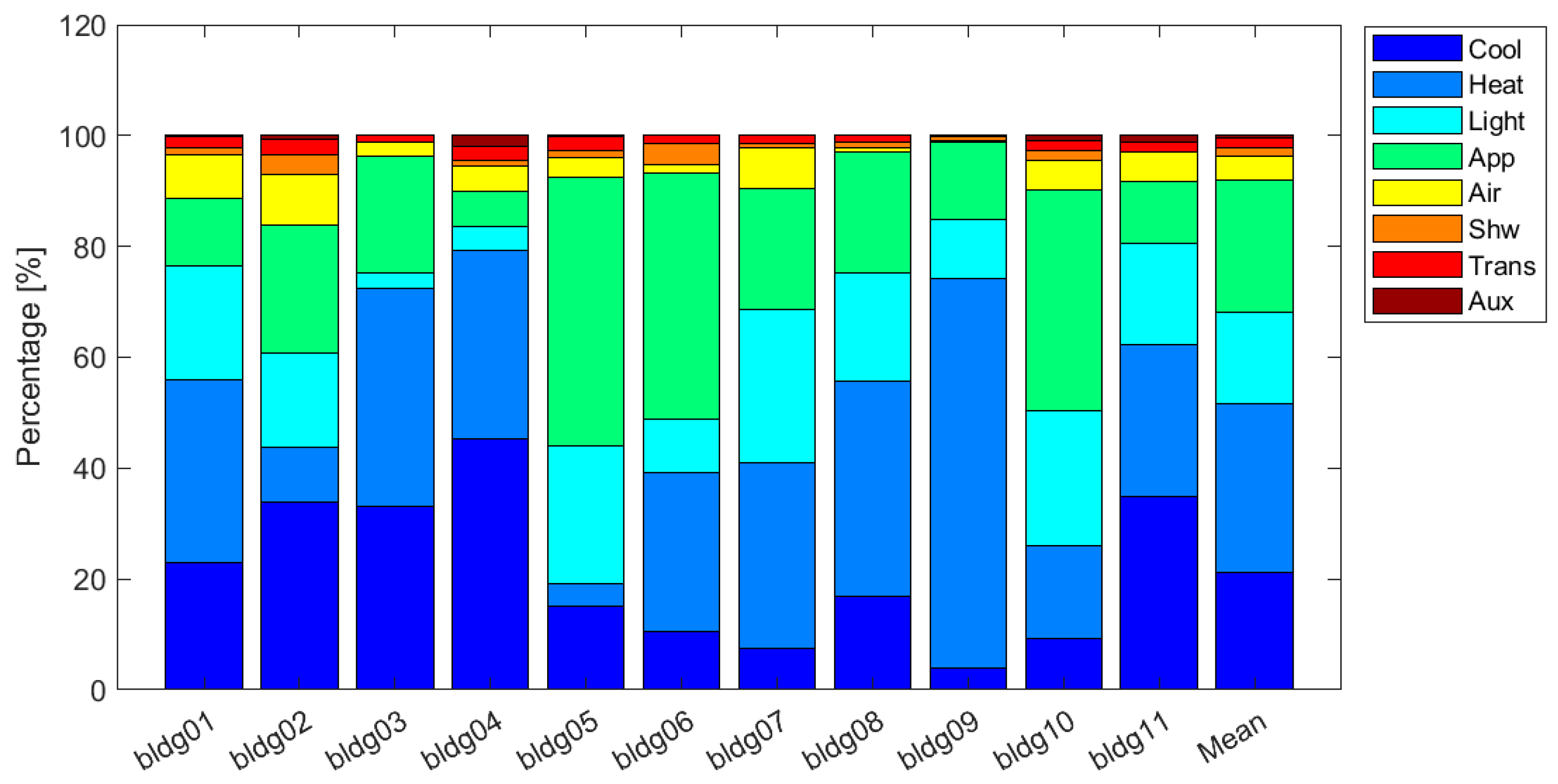
Figure 3 shows the ratio of the measured eight end-uses. The average ratios, denoted as Mean in Figure 3, of Cool, Heat, Light, App, Air, Shw, Aux, and Trans of the sample building are approximately 21%, 35%, 14%, 23%, 4%, 2%, and 1%, respectively.

In the case of bldg07 and bldg09, the percentage of heating and cooling use is outside the normal range; e.g., the ratio of Cool is very low at approximately 7.4% and 3.8%, while that for Heat is quite high at approximately 34% and 70%, respectively. Another case is bldg05, where the ratio of Heat is very low at approximately 4.1%; however, the ratio of App is approximately 48.5%, which seems to be quite large. Nearly all the buildings were equipped with a service hot water system (Table 1), but the ratio of Shw appears to be negligibly low, averaging 1.9%. Similarly, for most of the sampled buildings, the average ratios of Trans and Aux are also fairly low, with average values of approximately 1.7% and 0.6%, respectively. Refer to Appendix A for additional information on the descriptive statistics of each building.

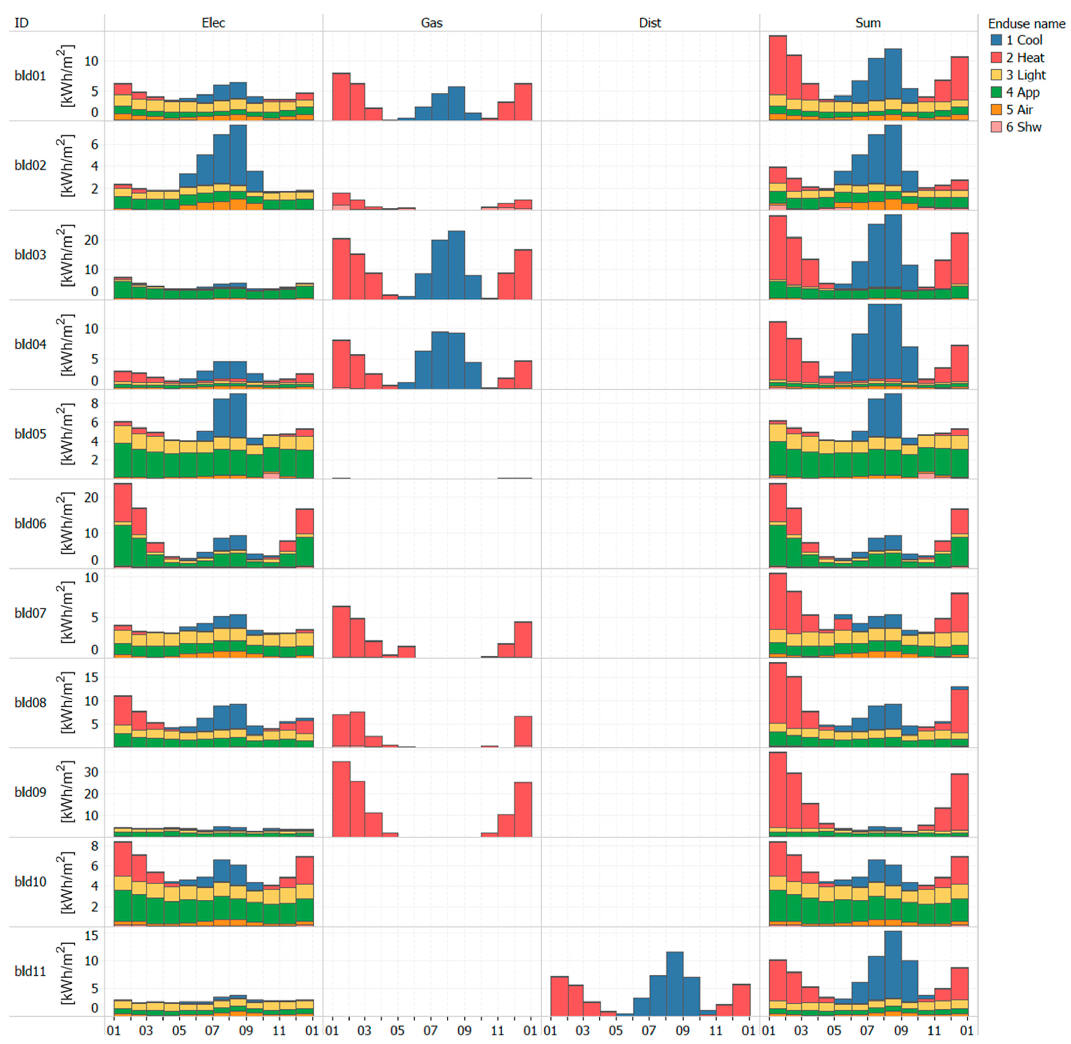
Figure 4 shows the monthly energy use by source (electricity, gas, and others) and the eight end-uses. All buildings demonstrated a very common pattern of up-and-down energy use. District heating or city gas for cooling is used in four buildings (bldg01, 03, 04, and 11); as advised by the Korean government, a cooling system using gas or district heating is used for certain-sized buildings to avoid peak electricity power. Meanwhile, three buildings (bldg06, 08, and 10) use electricity for heating. Additionally, auxiliary (Aux), indoor transportation (Trans), lighting (Light), and appliance (App) consumption does not change significantly throughout the year (Figure 4). Conversely, cool and heat clearly show seasonal patterns, and certain Air and Shw also show such trends. Such seasonal patterns of App, Air, and Shw increase the difference by acting as noise in the results of estimating seasonal usage of SED and CPR. For example, in the case of bldg01, 02, 07, 10, and 11, the Air ratio is 7.9%, 9.1%, 7.3%, 5.3%, and 5.4%, respectively, which is somewhat larger than that of other buildings (Figure 4).

Looking at the Sum pattern (the rightmost column in Figure 4), the time-series pattern can be classified into four types based on the consumption height in winter and summer: a heating and cooling load type (W-shape: bldg01, 03, 04, and 11), a heating load dominant type (U-shape: bldg06, 07, 08, and 09), a cooling load dominant type (A-shape: bldg02, 05), and a baseload dominant type (B-shape: bldg10). It can be expected that the SED and CPR estimation accuracy will vary according to these patterns. That is, in the case of having a distinct seasonal pattern such as the W-shape, the influence of noise (e.g., fluctuations in Air, Shw, App, and Light) on heating and cooling will be reduced and the estimation accuracy will be high. In the case of the U-shape, the noise influence on heating (cooling) usage will be decreased (increased). Similarly, in the case of the A-shape, the opposite applies. In the case of the B-shape, it is expected that the SED and CPR estimations will be less accurate because they are sensitively influenced by small fluctuations of the noises that are assumed to be stable.

2.3. Simplified Weather-Sensitive Energy Disaggregation (SED) Approach

The SED approach generates three quantities: summer-sensitive energy, winter-sensitive energy, and baseload energy. A brief graphical explanation of this method is presented in Figure 5 and Equations (1)–(4). In the figure, the y-axis indicates the EUI of a certain energy source, and the x-axis represents the month. In addition, $E{t}_i$, $E{c}_i$, $E{h}_i$, and $E{b}_i$ denote the total energy, cooling-related energy, heating-related energy, and baseload energy at month $i$, respectively, wherein the subscript $i$ denotes the $i^{th}$ month in {1,…,12}. $E{m}_s\left(1-\beta \right)$ denotes the deviation between $E{t}_f$ and $E{t}_s$. The subscript f indicates the month corresponding to the minimum value of $E{t}_i$, and the subscript $s$ indicates the month with the second-lowest value of $E{t}_i$. The values of f and s should be mutually and exclusively located in the shoulder season. Considering heating and cooling degree-days of each month in South Korea, f and s were set to be located in a range between March to May and September to November, respectively.

$$Eb=\left(E{t}_f+\beta ·E{m}_s\right)\times 12$$

(1)

$$Eh={{\displaystyle \sum }}_{i=1}^{f-1}[E{t}_i-(E{t}_f+\beta ·E{m}_s)]+{{\displaystyle \sum }}_{i=s+1}^{12}[E{t}_i-(E{t}_f+\beta ·E{m}_s)]+\frac{E{m}_s(1-\beta )}{2}$$

(2)

$$Ec={{\displaystyle \sum }}_{i=f+1}^{s-1}[E{t}_i-(E{t}_f+\beta ·E{m}_s)]+\frac{E{m}_s(1-\beta )}{2}$$

(3)

where

$$E{m}_s=E{t}_s-E{t}_f$$

(4)

In this study,$\beta$, denoting the baseload adjustment factor in Equations (1)–(3), is newly introduced; the closer to zero (one), the less (more) weight given to $Eb$ In previous studies [5,15,18], $\beta$ was set to zero; hence $Eb$ would be underestimated, but $Eh \mathrm{and} Ec$ were overestimated, when the consumption in one of the shoulder seasons is extremely small due to vacancy or vacation. Hence, such an adjustment factor is needed to alleviate the extreme small values (e.g., zero) of shoulder season consumption.

In this study, $\beta$ was set to 0.5 (averaging the height of two shoulder months, f and s) for stability. The monthly baseload ($E{t}_f+\beta ·E{m}_s$, right-hand side of Equation (1)) was calculated by averaging the two lowest monthly quantities considering shoulder seasons (f, s). The Weatherization Assistance Program [9,19] uses slightly different criteria to split the baseload, i.e., it calculates the baseload by averaging the three lowest quantities without considering shoulder seasons.

SED is premised on the naïve assumption that heating or cooling energy consumptions are negligibly small during the change in seasons (spring and autumn). Accordingly, if a building has year-long heating or cooling loads (e.g., hospitals, banks, and data centers), estimation errors will increase. This method, in particular, has advantages in terms of affordability and simplicity. The quantity (Ec and Eh) can be calculated even with abnormal fluctuations during heating or cooling seasons because it does not assume a linear relationship between heating (or cooling) energy and outdoor temperature. The outputs (Ec and Eh), however, are sensitive to unusually low values during shoulder seasons.

It should be noted that the SED is suitable for South Korea’s climate as the country experiences a temperate climate with four distinct seasons. In particular, winters (January and December) are typically cold and dry, whereas summers (July and August) are hot and humid. As shown in Figure 6, we can assume that the inflection points may occur from heating to cooling and from cooling to heating in the spring (March~May) and autumn (September~November), respectively. Based on this pattern, the cooling- (Ec) and heating-related (Eh) energy usage can be disaggregated by subtracting the minimum value, regarded as the base load energy (Eb), during the transition of seasons from the monthly EUI pattern. The peak heating and cooling energy consumption may differ depending on the building type (e.g., residential or commercial). A building that does not follow such a sinusoidal pattern may be regarded as an exceptional case (e.g., long vacancy or system failure).

2.4. Change-Point Regression (CPR) Approach

The CPR approach is among the widely used energy signature methods [17]. It utilizes historical monthly consumption data against average outdoor temperatures. The CPR, also known as piecewise linear regression model, is a de facto standard analysis approach often used in predicting heating and cooling energy sensitivity (or consumption) against outdoor temperature in residential and commercial buildings, specifically discussed in [20].

The physical basis of the linear change point methods is already established, and with appropriate interpretation, certain parameters such as the balance point temperature can be estimated. The model shapes considered for this algorithm include two- to five-parameter models (

Table 2. CPR models [17].

Model Type	Form	Description
One-parameter (1P)	E = b0	Non-weather-sensitive demand
Two-parameter (2P)	E = b0 + b1 T
Three-parameter (3P)
for heating	E = b0 + b1 (b2 − T)+	Seasonal weather-sensitive use (fuel in winter, electricity in summer for cooling)
for cooling	E = b0 + b1 (T − b2)+
Five-parameter (5P)	E = b0+ b1 (b3 − T)+ + b2 (T − b4)+	Heating and cooling supplied by same meter

T denotes monthly mean daily outdoor dry-bulb temperature. b₀, b₁, b₂, b₃, and b₄ represent parameters to be estimated for piecewise linear regression models. ()⁺ notation indicates a case in which the parenthetic term is set to 0 if it is evaluated as a negative number.

). In this study, the four-parameter model was excluded for simplicity of analysis.

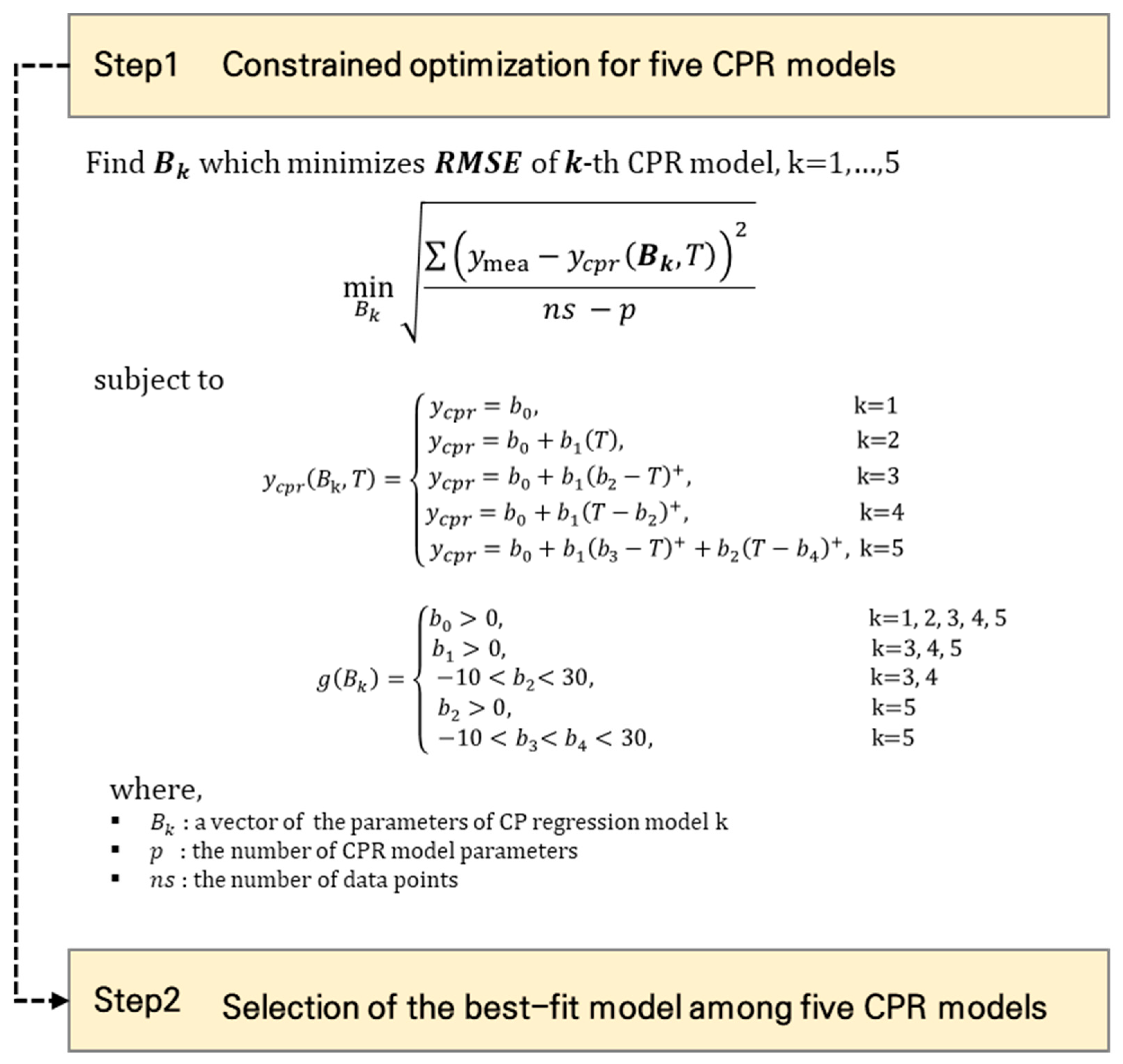
In this study, the optimal CPR model type is selected through the following steps (Figure 7).

• Step 1: constrained optimization is carried out to identify the best model coefficients ($B_k$) for each of the five different model types (k = 1,…,5). It comprises the constraint function for model coefficients ($\mathrm{g}\left(B_k\right)$) and the objective function for minimizing root-mean-squared error (RMSE) [16]. Constraints were set for each model coefficient to maintain its geometry.
• Step 2: the optimal model type with the lowest RMSE is chosen. By using the optimal model, heating and cooling energy consumption are predicted and summed to yearly values. All process is repeated at each energy source.

The only difference between our approach and the original approach is the optimization technique. In particular, our approach is based on the constraint optimization technique, while that of the original is based on a two-stage grid search algorithm [13,16,32]. The regression modeling and model type selection process were implemented in the MATLAB R2021a environment with the optimization toolbox.

3. Results

3.1. SED Outputs

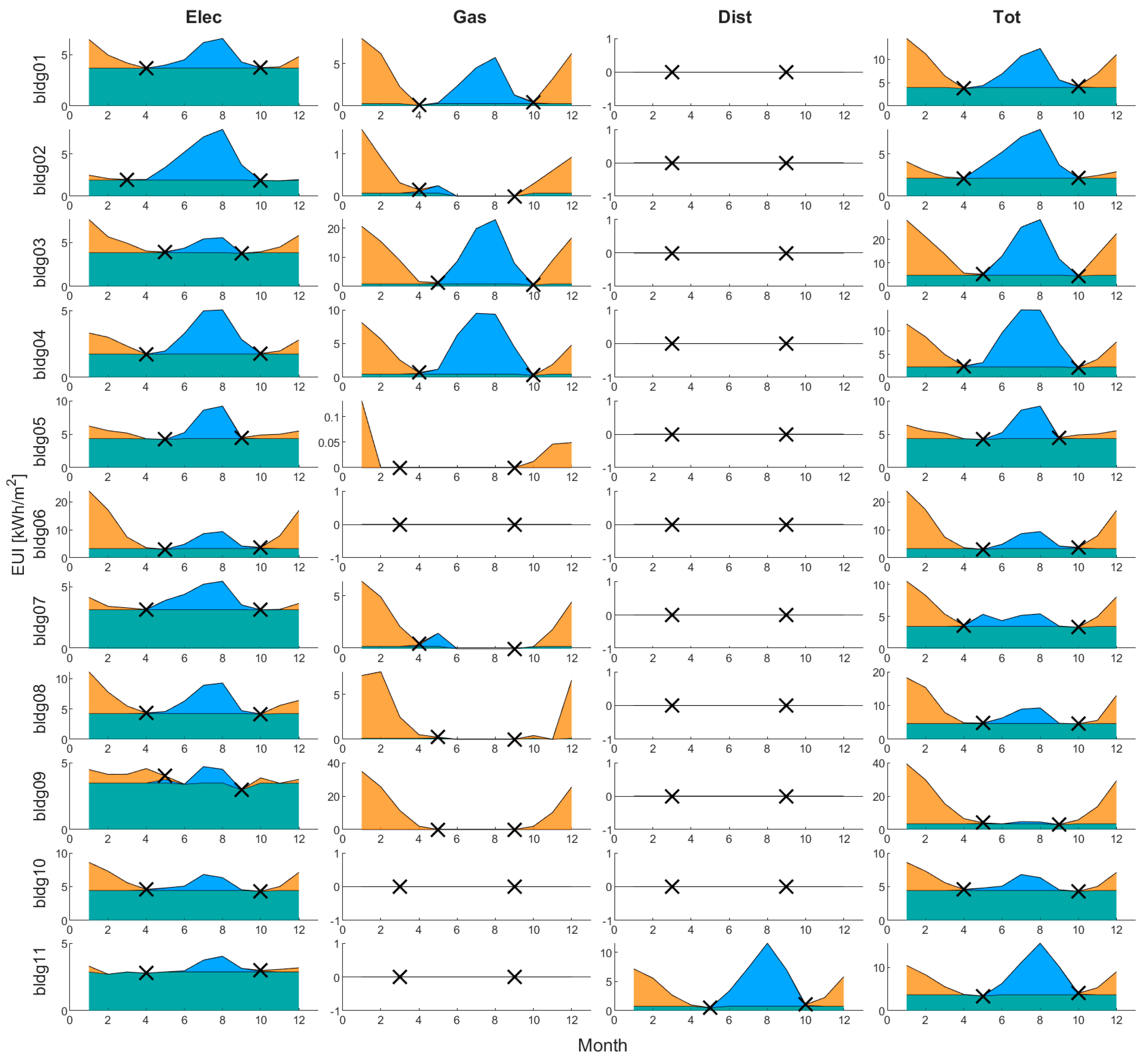
The disaggregation results of the SED approach are presented in Figure 8. The SED was sequentially applied to each monthly energy source (electricity, gas, district heating), and each output was summed to produce the total heating and cooling consumption of a building (Tot in Figure 8). All buildings showed a typical seasonal swing pattern in their energy use. The months with minimum electricity consumption were observed frequently for April (6 of 11: bldg01, 04, 07, 08, 10, and 11) and October (8 of 11: bldg01, 02, 04, 06, 07, 08, 10, and 11).

In the case of electricity use, seasonal variations were observed in most buildings, and the degree of rise and fall of energy use varied depending on whether the gas or district heat sources were used for cooling. Since bldg06 and 10 managed the heating loads with EHP, we observed a pattern of increasing electricity consumption during winter. In contrast, the use of absorption chiller–heaters significantly increased the amount of gas used in the summer (June–September) for bldg01, 03, and 04 (Table 1), excluding bldg07 in which the absorption chiller was not actively used.

In particular, bldg09 used more than 70% energy for heating by gas and less than 4% of energy for cooling, which represents a typical residential building consumption pattern. As bldg11 actively used district heating energy sources for managing both heating and cooling loads, it seemed that the seasonal variation of electricity consumption is minimal.

3.2. CPR Outputs

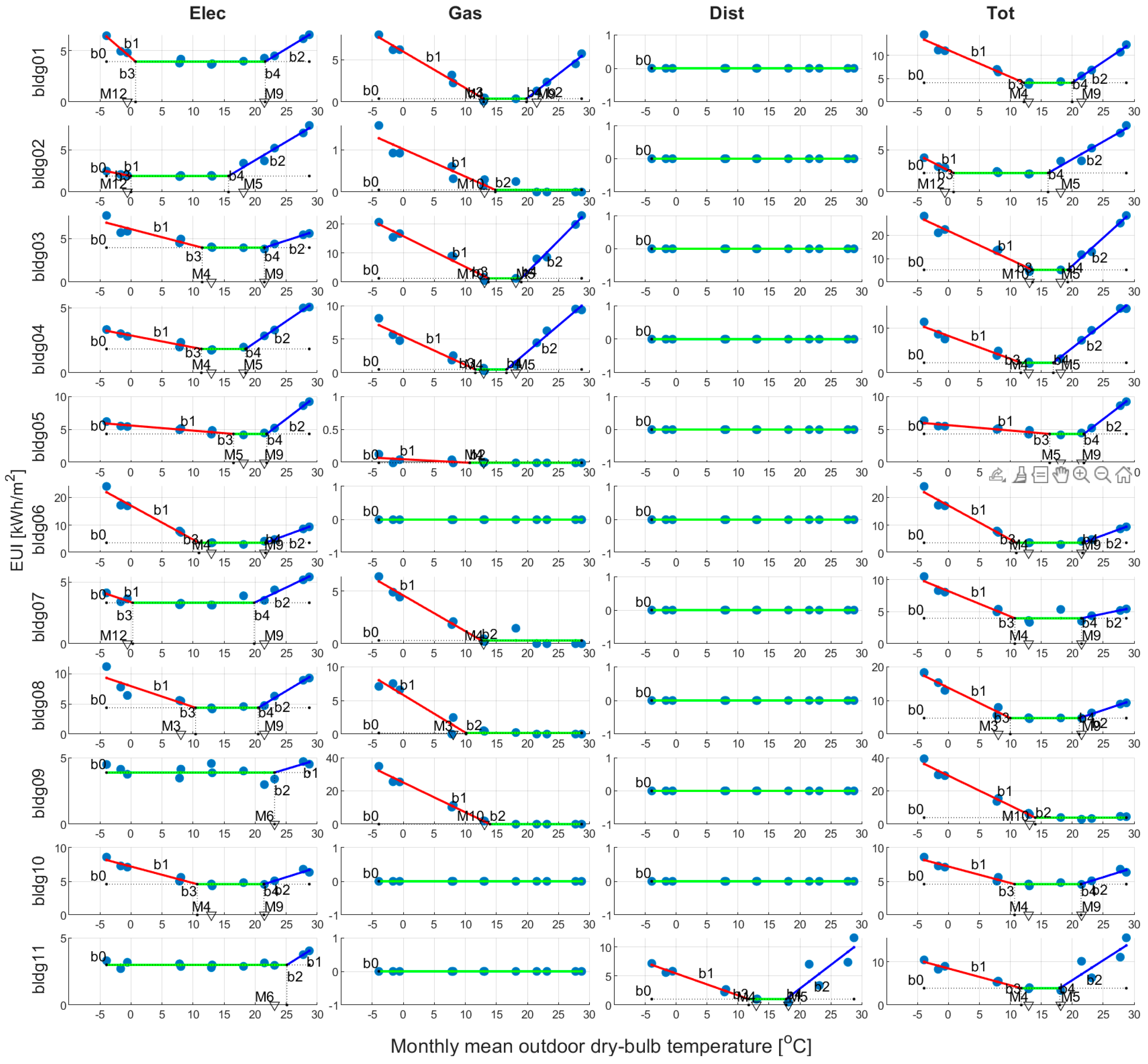
The CPR results are presented in Figure 9. The solid-blue line denotes the cooling slope, the solid-red line represents the heating slope, and the green line indicates the baseload (b₀). The change-point was denoted in the form of “M00” (e.g., the notation M10 indicates October).

The monthly pattern of electricity usage exhibited a distinct seasonal variation in most buildings (as shown in Figure 4 and Figure 8). As observed, the 5p model was mostly selected at the electricity source, except for bldg09 and 11. For bldg09 and 11, the 3p-cool model was selected because of the increase in electricity consumption in summer; however, it seems that 3p-cool model was barely chosen for bldg09.

At the gas energy source, the 5p model was selected frequently due to the heat-driven cooling system (e.g., absorption chiller): for bldg01, 03, and 04, which are equipped with an absorption chiller–heater, but not for bldg07 (Table 1). For bldg07, the absorption chiller was not actively used to manage the cooling load and the 3p-heat model was chosen. In particular, the 5p model was selected for bldg11, which actively uses district heating energy sources for managing both heating and cooling load.

Regarding the total energy use, the 5p model was expected for most buildings considering the target building type (office building), but for bldg09, the 3p-heat model was chosen. It is speculated that some cooling equipment may be operated sub-optimally or turned off, but further research is needed to draw definitive conclusions.

Detailed information on the model parameters is described in

Table 3. Parameters of the best-fit model by energy sources.

ID	Energy Source	CPR Type	b0a	b1b	b2c	b3d	b4e	R2
bldg01	Elec	5p	3.94	0.52	0.37	0.74	21.63	0.97
	Gas	5p	0.38	0.43	0.57	12.95	19.85	0.99
	Tot	5p	4.11	0.58	0.90	12.19	19.99	0.98
bldg02	Elec	5p	1.89	0.14	0.44	0.00	15.72	0.98
	Gas	3p_h	0.05	0.07	14.83	n/a	n/a	0.91
	Tot	5p	2.25	0.37	0.42	0.83	16.10	0.97
bldg03	Elec	5p	3.94	0.19	0.23	11.47	21.50	0.89
	Gas	5p	1.29	1.06	2.15	13.72	19.00	0.98
	Tot	5p	5.22	1.22	2.40	13.59	19.28	0.98
bldg04	Elec	5p	1.84	0.09	0.33	11.35	18.47	0.99
	Gas	5p	0.50	0.42	0.78	11.61	16.63	0.97
	Tot	5p	2.27	0.52	1.09	11.70	16.95	0.98
bldg05	Elec	5p	4.35	0.08	0.71	16.52	21.88	0.99
	Gas	3p_h	0.00	0.01	10.72	n/a	n/a	0.50
	Tot	5p	4.35	0.08	0.71	16.36	21.88	0.98
bldg06	Elec	5p	3.66	1.22	0.82	10.96	21.67	0.98
	Tot	5p	3.66	1.22	0.82	10.96	21.67	0.98
bldg07	Elec	5p	3.33	0.17	0.24	0.28	19.86	0.91
	Gas	3p_h	0.31	0.34	12.59	n/a	n/a	0.96
	Tot	5p	3.98	0.40	0.20	10.73	21.50	0.93
bldg08	Elec	5p	4.37	0.34	0.62	10.41	20.51	0.87
	Gas	3p_h	0.17	0.56	10.11	n/a	n/a	0.95
	Tot	5p	4.75	0.90	0.62	9.98	21.14	0.97
bldg09	Elec	3p_c	3.88	0.14	23.14	n/a	n/a	0.27
	Gas	3p_h	0.00	1.79	13.97	n/a	n/a	0.99
	Tot	3p_h	3.92	1.80	14.02	n/a	n/a	0.99
bldg10	Elec	5p	4.58	0.25	0.29	10.68	21.43	0.95
	Tot	5p	4.58	0.25	0.29	10.68	21.43	0.95
bldg11	Elec	3p_c	2.98	0.29	25.13	n/a	n/a	0.82
	Dist	5p	1.01	0.38	0.82	11.73	17.78	0.84
	Tot	5p	3.89	0.39	0.92	11.77	17.98	0.85

^a Unit: kWh/m², ^b Unit: kWh/m² °C, ^c Unit: for 3p °C or for 5p kWh/m² °C, ^d Unit: °C, ^e Unit: °C.

. Most of the models have an R² of 0.8 or higher, showing excellent explanatory power. As a special case, some models have bad R² values; for example, those for the gas model of bldg05 and the electric model of bldg09 are 0.5 and 0.27, respectively. It is presumed that the consumption itself is very small and the monthly consumption pattern is unstable for both cases (Figure 4 and Figure 8).

3.3. Group Difference in Approaches

One-way analysis of variance (ANOVA) tests were conducted to identify significant between approaches in cooling- and heating-related energy use. The factors were SED, CPR, and MEA. Before proceeding with the ANOVA tests, it was necessary to check whether the dataset was approximately normally distributed. The original dataset exhibited positive skew in all cases, and data were thus log-transformed to obtain an approximately normal distribution. Finally, a one-way ANOVA revealed that there was not a statistically significant difference between the three approaches (p-values were 0.821 and 0.980 for cooling and heating, respectively (

Table 4. ANOVA summary table for three approaches (SED, CPR, and MEA).

Variable		Sum of Squares	Df	Mean Square	F	Sig.
Cooling-related	Between groups	0.3406	2	0.1703	0.20	0.8212
	Within groups	25.7693	30	0.8589
	Total	26.1099	32
Heating-related	Between groups	0.0040	2	0.0216	0.02	0.9807
	Within groups	30.9801	30	1.0326
	Total	31.0205	32

)).

Figure 10 shows the distribution of log-transformed cooling and heating energy use among the three approaches. Indeed, the difference in distribution between the three methods appears to be negligible. However, in the case of cooling, the median of CPR is slightly lower; in the case of heating, the median of MEA is slightly higher but seems to be negligible.

Additionally, the Pearson correlation coefficient was measured for pair comparison. The Pearson correlation coefficient is commonly used for a measure of the strength of a linear association between two variables (X, Y) and is denoted by $r_{X,Y}$ (Equation (5)). The numerator is the covariance between the two variables, and the denominator is the product of the standard deviation of each variable. The correlation coefficient has a range of −1 to 1, with 0 denoting no association and 1 (−1) denoting a significantly positive (negative) correlation.

$$r_{X,Y}=\frac{{{\displaystyle \sum }}_i^n\left(X_i-\overline{X}\right)\left(Y_i-\overline{Y}\right)}{\sqrt{{{\displaystyle \sum }}_i^n{\left(X_i-\overline{X}\right)}^2}\sqrt{{{\displaystyle \sum }}_i^n{\left(Y_i-\overline{Y}\right)}^2}}$$

(5)

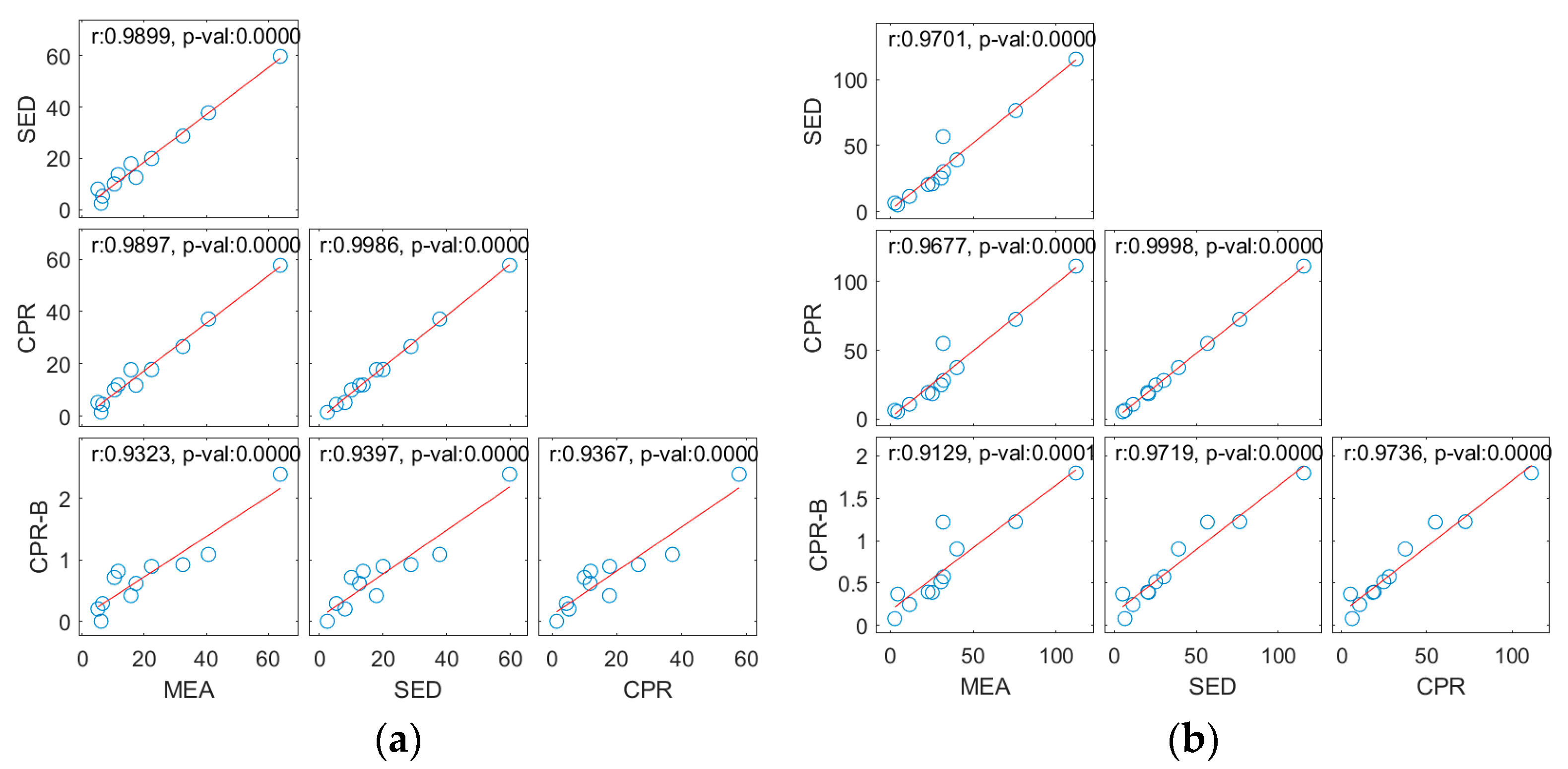
As shown in Figure 11, in the case of cooling-related energy, the correlation coefficients among the actual measurement and the estimation methods were more than 0.95 for all combinations (MEA vs. SED, MEA vs. CPR, and SED vs. CPR), which can be deemed a strong correlation. The same conclusion can be drawn for heating-related energy use (all r values of all combinations >0.95).

To check the correlation between the slope parameter (b₁ or b₂) of Total energy use by CPR (see Table 3) and SED outputs, the group CPR-B was included on purpose. Interestingly, the correlation between the SED and CPR-B was also very high (r = 0.939 for cooling, r = 0.971 for heating). This result implies that all methods (SED, CPR, MEA, and CPR-B) yield a very similar “rank” in the context of relative evaluation, e.g., benchmarking application, although they may not guarantee accuracy in terms of cooling- and heating-related energy quantity.

3.4. Errors in Estimation

For some buildings, there may be large or very small deviations between the measured values and the estimated heating- and cooling-related consumption. This section examines disaggregation differences at the individual building level perspective to gain insight into the cause of the difference.

The common metrics used for evaluating the estimation deviation include percentage error (PE), mean percentage error (MPE, or bias), and mean absolute percentage error (MAPE). These are defined as follows:

$$P{E}_i=\frac{\left(ME{A}_i-ES{T}_i\right)}{ME{A}_i}\times 100\%$$

(6)

$$MPE=\frac{1}{N}{\displaystyle \sum }_{i=1}^{N}P{E}_i$$

(7)

$$MAPE=\frac{1}{N}{{\displaystyle \sum }}_{i=1}^N\left|P{E}_i\right|$$

(8)

where $ME{A}_i$ and $ES{T}_{\mathrm{i}}$ are the $i$-th measurement and estimate, respectively. The MPE represents the mean estimation error, representing the systematic error of the model (e.g., SED and CPR) for under- or over-estimation. MAPE yields the average magnitude of estimation errors.

In

Table 5. Individual comparison among three approaches.

Experiment	ID	EUI [kWh/m2·yr]			PE [%]		Pattern Type 3
		MEA	SED 1	CPR 2	SED vs. MEA	CPR vs. MEA
Cooling-related	bldg01	22.4	20.0	17.8	−10.7	−20.6	W
	bldg02	15.7	17.9	17.7	13.9	12.6	A
	bldg03	63.9	59.7	57.7	−6.6	−9.7	W
	bldg04	40.7	37.7	37.1	−7.3	−8.8	W
	bldg05	10.4	10.1	10.0	−3.1	−3.8	A
	bldg06	11.6	13.7	11.9	18.4	2.7	U
	bldg07	5.1	8.0	5.2	59.1	3.1	U
	bldg08	17.4	12.6	11.8	−27.5	−32.2	U
	bldg09	6.1	2.5	1.4	−59.2	−76.6	U
	bldg10	6.6	5.3	4.5	−18.7	−32.2	B
	bldg11	32.5	28.7	26.6	−11.5	−18.1	W
Heating-related	bldg01	32.2	30.2	28.1	−6.3	−12.8	W
	bldg02	4.5	5.0	5.3	11.1	17.8	A
	bldg03	75.6	76.5	72.5	1.1	−4.1	W
	bldg04	30.7	25.3	24.8	−17.5	−19.0	W
	bldg05	2.8	6.4	6.3	131.1	127.0	A
	bldg06	31.9	56.8	55.0	77.9	72.4	U
	bldg07	22.9	20.5	19.3	−10.7	−15.9	U
	bldg08	40.2	39.1	37.4	−2.8	−6.9	U
	bldg09	111.9	115.5	111.3	3.2	−0.6	U
	bldg10	11.7	11.4	10.7	−2.4	−8.0	B
	bldg11	25.4	20.9	18.4	−17.9	−27.5	W

Note: ¹ Quantity is calculated by adding all estimated cooling-related energy uses by each energy source; ² Quantity is calculated by adding all predicted summer- or winter-sensitive energy uses by each energy source based on the optimal model; ³ W: heating and cooling load type, U: heating dominant load type, A: cooling dominant load type, B: baseload dominant type.

, the measured annual cooling and heating consumption (MEA) are presented along with the estimates obtained using the SED and CPR.

• Estimation in cooling-related energy: large PEs were observed for U- and B-shape buildings: bldg06, 07, 08, 09, and 10, regardless of SED and CPR. The absolute value of PE is in the range 18%–59%. This is significantly large compared to the W- and A-shape buildings (Figure 4), which have smaller PEs in the range between 3% and 14%. As mentioned in Section 2.2, such U- and B-shape types are weak by small fluctuations when estimating cooling energy use. The same is true for CPR: the largest PE was observed for U- and B-shape buildings. The absolute value of PE is in the range 3.1%–75.6%. Notably, the PE of bldg07 is small, but it seems that it happens by chance.
• Estimation in heating-related energy: as expected, the largest PE was observed for the A-shape building (bldg05). The absolute values of PE of SED and CPR are approximately 131% and 127.0%, respectively. Interestingly, bldg06, having a U-shape pattern, shows a relatively large error in SED and CPR (77.9% and 72.4%, respectively); the pattern of App shows seasonal variation, i.e., a W-shape as shown in Figure 4. One possible explanation is that the use of zone air conditioners or electric heaters was not fully controlled during the field measurement. The second reason is that energy end-uses of such zonal systems were mixed into “plug-load” branches and summed into the App category. This leads to seasonal fluctuations of the energy use of App, consequently leading to large errors. It should be noted that fully controlled measurement is difficult in practice; hence, it is necessary to analyze the results with these circumstances taken into account [36]. Since these measurement issues are outside the scope of this study, this was not addressed.

The MPEs of both approaches were under- and over-estimated for cooling and heating, by approximately −5%–17% and 15%–11%, respectively (

Table 6. Summary of overall errors.

Experiment	Metrics	SED vs. MEA	CPR vs. MEA
Cooling-related	MPE	−5%	−17%
	MAPE	21%	20%
Heating-related	MPE	15%	11%
	MAPE	26%	28%

). The MAPEs of both approaches are shown as 30% or less in both cooling and heating. Evidently, both approaches produce marginally better results in cooling than heating.

4. Discussion

4.1. Advantanges and Disadvantages of the Estimation Methods

As discussed in Section 3.3, there was no significant difference between the groups when comparing SED and CPR with the measured heating and cooling usage (Table 4), and the two had a high correlation with each other (Figure 11). Additionally, on average, the MPE and MAPE metrics were at an acceptable level, notwithstanding some inaccuracy as discussed in Section 3.4. Although there are methods that derive similar results, the advantages and disadvantages of each method are clear, so the points to be considered in actual use or interpretation are discussed:

• The processing algorithm for SED is light, can processes large datasets rapidly. Moreover, since it is a non-parametric approach, it can be implemented in Excel based on a simple calculation process. However, since the outdoor air temperature is not used, the correlation information between the outdoor air temperature and the energy consumption is lost. In addition, when it is necessary to compare the outputs between different climate regions, a weather normalization technique is needed. However, for CPR, such normalization is unnecessary because it already includes outdoor air temperature in the slope parameter.
• The advantage of the CPR method is that new information such as the balance temperature and slope parameter, and R², can be obtained. Such information can be used to determine the heating and cooling energy performance. For example, based on the balance temperature, it is possible to guess the relative internal heat gain (e.g., equipment) intensity level or the comfort level [31]. In the case of R², it is explanatory information for the outdoor temperature and, through this, the efficiency of operation of the building or the level of uncertainty in the behavior of occupants can be guessed. This information cannot be known through SED. In addition to the outdoor air temperature, other variables that affect energy consumption also can be considered. In other words, one of the primary benefits is that change-point multi-variable regression (CP-MVR) research has somewhat preceded it [20,26,31]. On the contrary, it requires an advanced analysis tool in which the optimization algorithm is run. As a result, the computation time may be relatively long. Another drawback is the finding that the optimal model process is sensitive to outliers. One or two outliers can lead to an upside-down shape, or a biased slope can be estimated [16]. To solve this problem, quantile regression [26] can be considered, but the complexity and difficulty increase. To use CPR more easily in practice, it is necessary to provide a special tool with increased usability in the government level. A representative example is the BETTER project [34].

4.2. Impact of Monthly Use Pattern in Estimation Error

Four monthly use patterns were classified (Figure 4 and Table 5). The W-shape is a heating and cooling load dominant type (bldg01, 03, 04, and 11); the U-shape is a heating load dominant type (bldg06, 07, 08, and 09); the A-shape is a cooling load dominant type (bldg02, and 05); and the B-shape is a baseload dominant type (bldg10). Such classification is intended to distinguish the strength of weather-sensitive energy. The more distinct shape is shown in terms of heating or cooling, and more accurate estimates are obtained. Hence, the estimation process is robust to noise (fluctuations of the remainders: App, Light, Air, etc.), and vice versa. Therefore, when using SED and CPR in practice, it is recommended to check the estimation reliability considering the four shapes. Although this study did not quantify the classification criteria of the four shapes, such shapes could be distinguished by calculating the amount of consumption in summer (or winter) divided by the amount of consumption in shoulder seasons (spring and autumn).

4.3. Implication of Strong Correlation of Each Approaches in Relative Evaluation

A strong correlation between the output values of SED, CPR, MEA, and CPR-B is shown in Figure 11. As mentioned in Section 3.3, the result implies that all methods yield very similar “ranks” in the context of relative evaluation (benchmarking). Specifically, the high correlation between SED, CPR, CPR-B, and MEA implies the possibility of mutual replacement. Regardless of the approach used, it can be expected that the relative evaluation rankings will be similar. When no detailed measurement database that supports establishing the target value or minimum requirement at the national level is available, the outputs of disaggregation approaches (SED or CPR) and weather-sensitive energy indicators can be used as alternative elements for constructing the benchmarking database. It is worth highlighting that a high correlation between the MEA and SED (or CPR) outputs does not imply high estimation accuracy. Therefore, it is necessary to use the SED, CPR, CPR-B, and MEA according to the given situation and purpose.

5. Conclusions and Limitations

The limitation of the total EUI to act as an energy performance indicator is that all end-uses are aggregated into one. This provides a crude indication of the energy performance. To obtain more indicative results, at least of weather-related energy end-uses, i.e., heating and cooling must be known. Such weather-sensitive quantities are more insightful for identifying the opportunities and prioritizing the potential actions for a more detailed analysis rather than total EUI.

For most small- and medium-sized buildings or low-income households, submetering by end-use is not feasible due to the expensive installation and management costs. The end-use data, especially for heating and cooling end-uses, of such buildings are a national blind spot. It is challenging to determine an adequate amount of energy use even when end-use data are gathered or submetered since there are no national benchmarks (goal values or minimum requirements) [5,8]. This issue is a major challenge faced by the South Korean government. In this context, this study investigated the two estimation approaches, SED and CPR, compared with the measurement dataset, MEA, from eleven office buildings.

In conclusion, SED and CPR estimated the amount of heating and cooling use appropriately compared with MEA. The result shows that the two approaches produce very similar outputs, and their outputs are strongly correlated. It implies the possibility of mutual complementation between the three approaches (SED, CPR, and MEA) for producing heating and cooling energy usage. However, it is important to note that these approaches have clear advantages and disadvantages, and thus should be used depending on the application context. The results are summarized as follows.

• Group differences. The ANOVA result showed that there was no significant difference among the three approaches of SED, CPR, and MEA. p-values were 0.821 and 0.980 for cooling and heating, respectively (Table 4).
• Correlation. A strong correlation of r = 0.97 or higher was found when the four groups (SED, CPR, CPR-B, and MEA) were compared for cooling and heating (Figure 11). This implies the possibility of mutual complementarity.
• Estimation accuracy. The MPEs of both approaches were over- and under-estimated by roughly −5%–17% and 15%–11%, respectively (Table 6). The MAPEs for cooling and heating were both found to be at or below 30%. It was shown that both approaches produce marginally better results in cooling than heating quantity.
• Individual differences in estimation error. It was found that the four monthly use patterns (W, U, A, and B-shape) had a significant impact on the estimation accuracy of the SED and CPR when comparing differences between individual buildings. The stronger (weaker) the weather-sensitive energy, the smaller (larger) the estimation error. As mentioned in Section 4.2, however, this study did not provide classification criteria for the four shapes. Further study is needed for quantifying classification.

Currently, the monthly energy consumption can be acquired on a nationwide scale (especially in South Korea) because of the National Building Energy integrated Database (NBED) [12,41,42]. The NBED is an integrated database in which the monthly energy database (from energy suppliers) is linked to the building registry (including address, completion year, primary space use, gross floor area, and number of floors, etc.). Therefore, cumulative frequency distributions of heating and cooling indicators for small- and medium-sized buildings in the NBED can easily be established by applying the SED or CPR when MEA is not feasible.

The findings of this study can be applied to NBED-like databases that have a wide geospatial range but a coarse (e.g., monthly) temporal interval. Therefore, it is envisaged that the practice of energy benchmarking will produce more actionable results by focusing on weather-sensitive energy (heating and cooling) rather than total use. This study was limited to eleven office buildings located in a temperate climate with four distinct seasons (Figure 6). Further study is needed considering larger sample sizes, and various building use types and characteristics.

References

1. Pérez-Lombard, L.; Ortiz, J.; González, R.; Maestre, I.R. A review of benchmarking, rating and labelling concepts within the framework of building energy certification schemes. Energy Build. 2009, 41, 272–278. [Google Scholar] [CrossRef]
2. Borgstein, E.H.; Lamberts, R.; Hensen, J.L.M. Evaluating energy performance in non-domestic buildings: A review. Energy Build. 2016, 128, 734–755. [Google Scholar] [CrossRef]
3. Mathew, P.; Mills, E.; Bourassa, N.; Brook, M. Action-oriented benchmarking: Using the CEUS database to benchmark commercial buildings in California. Energ. Eng. 2008, 105, 6–18. [Google Scholar] [CrossRef] [Green Version]
4. Chung, W. Review of building energy-use performance benchmarking methodologies. Appl. Energy 2011, 88, 1470–1479. [Google Scholar] [CrossRef]
5. Kim, D.W.; Kim, Y.M.; Lee, S.E. Development of an energy benchmarking database based on cost-effective energy performance indicators: Case study on public buildings in South Korea. Energy Build. 2019, 191, 104–116. [Google Scholar] [CrossRef]
6. Zhai, Z.; Salazar, A. Assessing the implications of submetering with energy analytics to building energy savings. Energy Built Environ. 2020, 1, 27–35. [Google Scholar] [CrossRef]
7. Wang, S.; Yan, C.; Xiao, F. Quantitative energy performance assessment methods for existing buildings. Energy Build. 2012, 55, 873–888. [Google Scholar] [CrossRef]
8. Katipamula, S.; Underhill, R.M.; Goddard, J.K.; Taasevigen, D.J.; Piette, M.A.; Granderson, J.; Kuruganti, T. Small- and Medium-Sized Commercial Building Monitoring and Controls Needs: A Scoping Study (No. PNNL-22169, 1063081); Pacific Northwest National Laboratory (PNNL): Richland, WA, USA, 2012.
9. Gov, n.d. About the Weatherization Assistance Program. Available online: https://www.energy.gov/eere/wap/about-weatherization-assistance-program (accessed on 16 June 2022).
10. Sesana, M.M.; Salvalai, G. A review on building renovation passport: Potentialities and barriers on current initiatives. Energ. Build. 2018, 173, 195–205. [Google Scholar] [CrossRef] [Green Version]
11. Sesana, M.M.; Rivallain, M.; Salvalai, G. Overview of the available knowledge for the data model definition of a building renovation passport for non-residential buildings: The ALDREN Project Experience. Sustainability 2020, 12, 642. [Google Scholar] [CrossRef] [Green Version]
12. Ji, C.; Choi, M.; Hong, T.; Yeom, S.; Kim, H. Evaluation of the effect of a building energy efficiency certificate in reducing energy consumption in Korean apartments. Energy Build. 2021, 248, 111168. [Google Scholar] [CrossRef]
13. Kissock, J.K.; Haberl, J.S.; Claridge, D.E. Development of a Toolkit for Calculating Linear, Change-Point Linear and Multiple-Linear Inverse Building Energy Analysis Models, ASHRAE Research Project 1050-RP [Final Report]; Energy Systems Laboratory, Texas A&M University: College Station, TX, USA, 2002. [Google Scholar]
14. Pereira, L.; Nunes, N. Performance Evaluation in Non-Intrusive Load Monitoring: Datasets, Metrics, and Tools—A Review. WIREs Data Min. Knowl. Discov. 2018, 8, e1265. [Google Scholar] [CrossRef] [Green Version]
15. Ahn, K.U.; Shin, H.S.; Park, C.S. Energy analysis of 4625 office buildings in South Korea. Energies 2019, 12, 1114. [Google Scholar] [CrossRef] [Green Version]
16. Paulus, M.T.; Claridge, D.E.; Culp, C. Algorithm for automating the selection of a temperature dependent change point model. Energy Build. 2015, 87, 95–104. [Google Scholar] [CrossRef]
17. ASHRAE. Handbook: Fundamentals 2017; American Society of Heating, Refrigerating and Air Conditioning Engineers: Atlanta, GA, USA, 2017. [Google Scholar]
18. Ji, C.; Hong, T.; Kim, H.; Yeom, S. Effect of Building Energy Efficiency Certificate on Reducing Energy Consumption of Non-Residential Buildings in South Korea. Energy Build. 2022, 255, 111701. [Google Scholar] [CrossRef]
19. Energy Auditor—Single Family 2.0: Utility Bill Analysis. Available online: https://www.energy.gov/eere/wap/downloads/energy-auditor-single-family-20-utility-bill-analysis (accessed on 29 September 2022).
20. Haberl, J.S.; Cho, S. Literature Review of Uncertainty of Analysis Methods (Inverse Model Toolkit), Report to the Texas Commission on Environmental Quality; Energy Systems Laboratory, Texas A&M University: College Station, TX, USA, 2004. [Google Scholar]
21. Oh, S.; Kim, K.H. Change-Point Modeling Analysis for Multi-Residential Buildings: A Case Study in South Korea. Energy Build. 2020, 214, 109901. [Google Scholar] [CrossRef]
22. Prahl, D.; Beach, R. Analysis of Pre-Retrofit Building and Utility Data; National Renewable Energy Lab. (NREL): Golden, CO, USA, 2014.
23. Park, J.S.; Lee, S.J.; Kim, K.H.; Kwon, K.W.; Jeong, J.-W. Estimating Thermal Performance and Energy Saving Potential of Residential Buildings Using Utility Bills. Energy Build. 2016, 110, 23–30. [Google Scholar] [CrossRef]
24. Eriksson, M.; Akander, J.; Moshfegh, B. Investigating Energy Use in a City District in Nordic Climate Using Energy Signature. Energies 2022, 15, 1907. [Google Scholar] [CrossRef]
25. Aragon, V.; James, P.A.B.; Gauthier, S. The Influence of Weather on Heat Demand Profiles in UK Social Housing Tower Blocks. Build. Environ. 2022, 219, 109101. [Google Scholar] [CrossRef]
26. Meng, Q.; Xiong, C.; Mourshed, M.; Wu, M.; Ren, X.; Wang, W.; Li, Y.; Song, H. Change-point multivariable quantile regression to explore effect of weather variables on building energy consumption and estimate base temperature range. Sustain. Cities Soc. 2020, 53, 101900. [Google Scholar] [CrossRef]
27. Kissock, J.K.; Reddy, T.A.; Claridge, D.E. Ambient-temperature regression analysis for estimating retrofit savings in commercial buildings. J. Sol. Energy Eng. Trans. ASME 1998, 120, 168–176. [Google Scholar] [CrossRef]
28. Ruch, D.; Claridge, D.E. A Four-Parameter Change-Point Model for Predicting Energy Consumption in Commercial Buildings. J. Sol. Energy Eng. 1992, 114, 77–83. [Google Scholar] [CrossRef]
29. Burak Gunay, H.; Shen, W.; Newsham, G.; Ashouri, A. Detection and Interpretation of Anomalies in Building Energy Use through Inverse Modeling. Sci. Technol. Built Environ. 2019, 25, 488–503. [Google Scholar] [CrossRef]
30. Kissock, J.; Seryak, J. Understanding Manufacturing Energy Use Through Statistical Analysis. In Proceedings of the Industrial Energy Technology Conference, Houston, TX, USA, 21–22 April 2004. [Google Scholar]
31. Golden, A.; Woodbury, K.; Carpenter, J.; O’Neill, Z. Change Point and Degree Day Baseline Regression Models in Industrial Facilities. Energy Build. 2017, 144, 30–41. [Google Scholar] [CrossRef] [Green Version]
32. Kissock, J.K.; Haberl, J.S.; Claridge, D.E. Inverse Modeling Toolkit: Numerical Algorithms, Ashrae KC-03-2-1(RP-1050); American Society of Heating, Refrigerating and Air Conditioning Engineers: Atlanta, GA, USA, 2003. [Google Scholar]
33. Haberl, J.; Sreshthaputra, A.; Claridge, D.; Kissock, J. Inverse Model Toolkit: Application and Testing. KC-03-02-2(RP-1050); American Society of Heating, Refrigerating and Air Conditioning Engineers: Atlanta, GA, USA, 2003. [Google Scholar]
34. Szum, C.; Zhou, N.; McQuillen, D.; Ding, C.; Li, H. Johnson Publishing Controls, Inc.: Han, & USDOE. (2021, July 27). In Building Efficiency Targeting Tool for Energy Retrofits (BETTER) Web Application (BETTER Web App) v.1.0; Computer Software; Lawrence Berkeley National Lab. (LBNL): Berkeley, CA, USA, 2021. [Google Scholar] [CrossRef]
35. Li, H.; Szum, C.; Nesler, C.; Lisauskas, S.; Snyder, S. Targeting Building Energy Efficiency Opportunities: An Open-Source Analytical and Benchmarking Tool. In Proceedings of the ASHRAE Winter Conference, Atlanta, GA, USA, 12–16 January 2019. [Google Scholar]
36. Healy, W. Measurement Challenges in Achieving Energy Monitoring Systems in Buildings, Technical Note (NIST TN), National Institute of Standards and Technology, Gaithersburg, MD, [online]. 2010. Available online: https://tsapps.nist.gov/publication/get_pdf.cfm?pub_id=904372 (accessed on 14 September 2022).
37. International Standard Organization (ISO). ISO12655; Energy Performance of Buildings—Presentation of Measured Energy Use of Buildings. International Organization for Standardization: Geneva, Switzerland, 2013.
38. KIAEBS. Methods for Classification, Measurement and Normalization of Energy Consumption by End-Use in Office Buildings; Korean Institute of Architectural Sustainable Environment and Building Systems: Seoul, South Korea, 2016. [Google Scholar]
39. Song, S.-Y.; Jin, H.-S.; Ha, S.-Y.; Kim, S.-I.; Kim, Y.-J.; Lee, S.-J.; Suh, I.-A. Detailed Office Building Energy Information Based on In Situ Measurements. Energies 2020, 13, 3050. [Google Scholar] [CrossRef]
40. KMA Weather Data Service. Available online: https://data.kma.go.kr/resources/html/en/aowdp.html (accessed on 1 September 2022).
41. Cho, M.S.; Le, D.Y. An Analysis of Residential Building Energy Consumption Using Building Energy Integrated Database—Focused on Building Uses, Regions, Scale and the Year of Construction Completion. J. Real Estate Anal. 2017, 3, 101–118. [Google Scholar] [CrossRef]
42. Ji, C.-Y.; Choi, M.-S.; Gwon, O.-I.; Jung, H.-R.; Shin, S.-E. Greenhouse gas emissions from building sector based on national building energy database. J. Archi. Inst. Korea Struct. Constr. 2020, 36, 143–152. [Google Scholar]
Figure 1. Research flowchart.
Buildings 12 01717 g001
Figure 2. Measured end-uses.
Buildings 12 01717 g002
Figure 3. Ratio of the end-use consumption. Cool: space cooling, Heat: space heating, Light: lighting, App: office electric appliances, Air: air movement by fans, Shw: domestic hot water, Aux: building auxiliary devices, Trans: indoor transportation, Mean: the mean value of the eleven buildings.
Buildings 12 01717 g003
Figure 4. Monthly energy end-uses profiles of eleven buildings (Elec: electricity, Gas: city gas, Dist: district heating).
Buildings 12 01717 g004
Figure 5. Monthly energy usage patterns in a temperate climate with four distinct seasons.
Buildings 12 01717 g005
Figure 6. Daily mean outdoor air temperatures in 2018 in Seoul, South Korea. Source: KMA Weather Data Service [40].
Buildings 12 01717 g006
Figure 7. Procedure overview for selecting the optimal CPR model type.
Buildings 12 01717 g007
Figure 8. SED results by energy sources (blue: E c ; orange: E h ; green: E b ). The markers (X) are estimated shoulder points (f, s) at spring and autumn seasons.
Buildings 12 01717 g008
Figure 9. CPR results by energy sources (blue: cooling slope, red: heating slope, green: baseload).
Buildings 12 01717 g009
Figure 10. Distribution of log of estimates (SED, CPR) and measurement (MEA).
Buildings 12 01717 g010
Figure 11. Correlation matrix among three approaches (SED, CPR, and MEA) plus CPR-B, which is a slope parameter (b1 or b2) based on Total energy consumption (Table 3): (a) cooling-related energy use; (b) heating-related energy use.
Buildings 12 01717 g011