Calibration of the Length of the Plastic Hinge for Numerical Models of Reinforced Concrete Members

Abstract

A proper and computationally efficient numerical modeling of the nonlinear cyclic flexural behavior of reinforced concrete members is crucial for the assessment of the seismic response of RC framed structures. To mitigate the problem of damage localization and improve the stability of the numerical model, force beam column elements with fiber cross-section and finite length hinges located at the ends of the member are often used. In this case, the accuracy in the prediction of the cyclic response is strictly dependent on the length assigned to the plastic hinge. In the past, several authors have proposed formulations to evaluate this crucial parameter based on observations and data from laboratory tests. Nevertheless, the values given by these expressions can differ significantly from each other. In this paper, the optimal value for the length of the plastic hinge is calibrated by comparison between laboratory and numerical test results. Laboratory tests are selected to identify members that are representative of columns of existing reinforced concrete buildings. Based on the optimal values of the plastic hinge length found for the selected set of laboratory tests, a simple relation of the plastic hinge length has been proposed.

1. Introduction

Numerical modeling of Reinforced Concrete (RC) members is a key factor for the seismic assessment of the RC structures. To investigate the inelastic behavior of beams and columns, these members are usually modeled by means of one-dimensional concentrated or distributed plasticity elements. In modeling of framed structures, concentrated plasticity models with plastic hinges of finite length are often preferred to distributed plasticity models to limit the damage localization problems and improve the computational efficiency. Concentrated plasticity elements have two plastic hinges at the ends and an elastic part in the middle. The geometry and the mechanical characterization of the plastic hinges, in particular the length L_pl of the plastic hinges, are of outmost importance for the accuracy of the response of RC members as they govern the load carrying and deformation capacities, as well as the energy dissipation of the member. In the past, several authors proposed formulations for the prediction of the length of the plastic hinge of RC members based on laboratory tests. However, large discrepancies exist among the results of these formulations, mainly because the inelastic behavior of materials is not discontinuous in real members and because different criteria may be considered to identify the length of the plastic hinge.

According to these formulations, several factors contribute to the value of L_pl, e.g., the shear span of the member, the depth of the cross-section, the mechanical properties of concrete (e.g., compressive strength, elastic modulus, compressive fracture energy), the geometric and mechanical properties of the longitudinal and transverse reinforcements (e.g., geometric percentage of steel bars and yield strength of steel), the effectiveness of confinement in the volume of the plastic hinge, and the axial force and the shear force. This makes the research for an analytical expression of the length of the plastic hinge an issue that is still open today.

Most of the proposed formulations are empirical in nature and calibrated against data obtained from laboratory experiments [1].

In 1956, Baker [2] elaborated a formula based on an experimental campaign consisting of 94 tests on beams and columns. The main variables considered were the compressive strength of concrete (f_c), the yield stress of the longitudinal rebars (f_yl), and the cross-sectional area of the longitudinal reinforcements in tension and in compression and the normalized axial force (i.e., the ratio of the axial force to the resisting axial force of concrete in the cross-section). According to Baker, the value of L_pl can vary between 0.4 d and 2.4 d (where d is the effective depth of the cross-section) in flexural members characterized by usual values of the shear span ratio L_v/d.

Later, from 1964 to 1967, Mattock [3,4] drew up two proposals based on 37 experimental tests on beams. In his experimental campaign, he took into account the compressive strength of concrete (f_c = 28 ÷ 41 MPa), the effective depth of the cross-section (25.4 ÷ 50.8 cm), the shear span ratio L_v/d (2.75 ÷ 11), the yield strength of the longitudinal reinforcement f_yl (324÷414 MPa) and its geometric percentage (ρ_l = 1.0 ÷ 3.0%). The same author stated that the spreading of the inelastic behavior along the element increases with the ratio L_v/d.

In 1982, Park et al. [5] performed tests on four square-section columns with L_v/h = 2.0 (where h is the depth of the cross-section) and normalized axial force ν between 0.2 and 0.6. The authors concluded that the normalized axial force does not play a significant role for the determination of L_pl and proposed, for columns, the use of a single value of L_pl = 0.4 h. In a similar way, from 1993 to 1998, Sheikh et al. [6,7,8] conducted other laboratory tests (mostly characterized by high values of the normalized axial force) and observed that the length of the plastic hinge L_pl was approximately equal to h.

In 1987, Priestley and Park [9] proposed a formula that depends on the length of the element and on the diameter of the longitudinal rebars. Later, in 1992, Paulay and Priestley [10] modified the previous equation to take into account the yield strength of steel. They stated that L_pl = h/2 can generally be assumed for typical columns.

In 2001, Mendis [11] conducted laboratory tests on 13 simply-supported beams and 4 columns with low axial force. He concluded that L_pl increases with the shear span ratio L_v/d and the geometric percentage of longitudinal reinforcement ρ_l, whereas it decreases with the increase of the geometric percentage of the transverse reinforcement ρ_v. Based on the tests on columns, Mendis stated that the length of the plastic hinge is not influenced by the axial force.

In 2008, Bae and Bayrak [12] performed tests on four squared columns with L_v/h ranging from 5 to 7 and normalized axial force ranging from 0.2 to 0.5. They proposed a procedure to evaluate L_pl under conditions of purely flexural behavior of the element. Through this procedure, validated on the tested columns, the authors performed a parametric analysis to establish that the parameters that mostly influenced L_pl are the normalized axial force ν, the shear span ratio L_v/h and the geometric ratio of the longitudinal reinforcement ρ_l. In particular, according to Bae and Bayrak, the length L_pl increased with the normalized axial force ν, the aspect ratio L_v/h and ρ_l.

More recently, Fardis et al. [13,14,15] proposed two empirical formulations of L_pl for members with axial force, in the presence of monotonic and cyclic load conditions. The proposed expressions primarily depended on the depth of the cross-section, the shear span ratio and the normalized axial force.

Although there is some agreement between the conclusions of the research studies aiming at the evaluation of the length of the plastic hinge (e.g., the influence of parameters such as the shear span ratio L_v/h or the height of the section), there are still some contrasting opinions regarding the influence of some parameters (e.g., the volumetric ratio of transverse reinforcement is considered to be relevant only by Mendis [11]). In addition, some of the parameters that are considered in the experiments (e.g., mechanical characteristics of materials, normalized axial force) still do not appear in most formulas.

In this scenario, a new formulation of L_pl is proposed here for columns that are common in existing RC framed buildings built in Italy between the 1970s and early 2000s. The optimal length of the plastic hinge is derived from comparison between the cyclic response of laboratory tests and results from numerical simulations. To this end, the authors have first examined the formulations proposed in the literature for the numerical modeling of materials and members. Based on this study, the authors have selected specified formulations of the material and member models and proposed some modifications to the usual simulation of concrete confinement. Second, a set of 33 experimental tests has been collected among those available in the literature. The selected columns have rectangular section and have failed in a flexural mode without slipping of the steel bars. Then, for each test, the value of the plastic hinge length has been calibrated so that the response of the numerical model be as close as possible to that of the laboratory test, in terms of energy dissipation and aspect of the lateral force—lateral displacement plot. Based on the obtained optimal values of the length of the plastic hinge, a relationship has been searched between the optimal value of L_pl and the geometric and mechanical characteristics of the specimens. The proposed relation is simple and reveals to be able to reproduce with satisfying accuracy the results of the considered experimental tests. The validity of this relation is restricted to the investigated ranges of the geometric and mechanical parameters and to the use of the assumed models of materials and members.

2. Modeling of Materials

2.1. Concrete

The uniaxial response of unconfined and confined concretes is simulated by means of the uniaxial material model “Concrete04” implemented in OpenSees [16]. Based on preliminary numerical tests conducted using others concrete material models (e.g., ConcreteCM), it has been found that the material model Concrete04 represents a good compromise between accuracy in the simulation of the cyclic response of concrete and numerical stability of the model.

2.1.1. Unconfined Concrete

The monotonic response of unconfined concrete under negative axial strains (shortening) is equal to that proposed by Mander et al. [17]. The value of the compressive strength f_c is equal to the mean value reported by the authors of the laboratory tests, whereas the modulus of elasticity is assumed equal to the value proposed by Chang and Mander [18]:

$$E_{\mathrm{c}}=8200f_{\mathrm{c}}^{3/8} (f_{\mathrm{c}} \mathrm{in} \mathrm{MPa})$$

(1)

The axial strain ε_c0, corresponding to the peak compressive strength, is given by the expression proposed by Chang and Mander [18]. It should be noted that the expression reported below has been converted from the original formula (expressed in psi):

$${\mathsf{\epsilon }}_{\mathrm{c}0}=\frac{f_{\mathrm{c}}^{1/4}}{1153} (f_{\mathrm{c}} \mathrm{in} \mathrm{MPa})$$

(2)

Loading and unloading paths follow the rules proposed by Karsan and Jirsa [19], i.e., they are linear, but their slope decreases with the increase in the axial strain. The monotonic response under positive axial strains (elongation) is described by an initially linear function and by a nonlinear softening branch with a degradation exponential function. The loading and unloading paths are linear with the slope equal to the secant stiffness at the point where the unloading path takes place. The tensile strength f_ct is evaluated as a function of the compressive strength f_c by means of the following relation:

$$f_{\mathrm{ct}}=0.30{\left(f_{\mathrm{c}}-8\right)}^{2/3} (f_{\mathrm{c}} \mathrm{in} \mathrm{MPa})$$

(3)

The above equation is recommended in Eurocode 2 [20] for concrete of strength classes ≤C 50/60 and is adequate for the simulation of the cyclic response of the specimens considered in this paper, as shown in successive sections. To ensure higher stability to the numerical analyses, the ultimate compressive strain of the unconfined concrete ε_cu is assumed to be fairly high and equal to 2%. This choice does not influence the accuracy of the global response appreciably because the post-peak branch of the stress-strain law of the unconfined concrete is rather steep and thus the compressive stress corresponding to high values of strain is low.

2.1.2. Confined Concrete

The compressive strength of confined concrete f_cc is evaluated according to the confinement model proposed by Chang and Mander [18,21] whereas the modulus of elasticity E_cc is obtained by Equation (1) as a function of f_cc. The slope of the softening branch of the monotonic compressive response of the “Concrete04” material is strongly influenced by the strain ε_cc0 corresponding to the peak compressive stress f_cc. The strain ε_cc0 is calibrated here so that the stress resulting from the “Concrete04” model at a strain of 3 ε_cc0 be equal to the value f_f suggested by Chang and Mander [18] for the same value of strain (see Appendix A). The parameters related to the response in tension are equal to those assumed for the unconfined concrete.

The ultimate compressive strain of confined concrete ε_ccu is assumed equal to three times the value that Priestley et al. [22] suggested on the basis of tests on members subjected to axial force only. A similar increment was also proposed by Scott et al. [23] in members subjected to combined axial force and bending moment in order to consider the strain gradient in the cross-section. Therefore, the ultimate compressive strain assumed here for confined concrete is

$${\mathsf{\epsilon }}_{\mathrm{ccu}}=3\cdot \left[0.004+1.4\hspace{0.17em}{\mathsf{\rho }}_{\mathrm{vol},\mathrm{st}}\left(\frac{f_{\mathrm{y},\mathrm{st}}\hspace{0.17em}{\mathsf{\epsilon }}_{\mathrm{su}}}{f_{\mathrm{cc}}^{}}\right)\right]$$

(4)

where f_y,st, ε_su and ρ_vol,st are, respectively, the yield stress, the ultimate strain and the volumetric ratio of the transverse reinforcement.

2.2. Steel

The uniaxial response of the steel bars has been modeled by means of the material model “Reinforcing Steel” implemented in the program Opensees [16]. This model [17,24] takes account of the Bauschinger effect and considers isotropic and kinematic hardening of steel. In addition, the model allows the simulation of buckling [25,26] and fatigue phenomena of steel rebars [27].

In the following numerical analyses, the modulus of elasticity is assumed equal to 210,000 MPa whereas the yield and ultimate stress (and the ultimate strain, if reported) are obtained from the papers written by the authors of the laboratory tests. Strain and tangent at initial strain hardening have been calibrated as a function of the main mechanical characteristics of the steel bars. Isotropic hardening has been neglected owing to the absence of data able to accurately define this effect in the considered experimental tests. After an initial phase of the research in which buckling and fatigue of steel bars have been considered, the authors have decided to neglect these phenomena in the examined specimens in order to facilitate numerical convergence. It is the opinion of the authors that consideration of buckling and fatigue may be important for the simulation of some tests but that their implementation in existing material models needs further investigation to produce general improvement in the accuracy of the response.

3. Modeling of the Cross-Section

This section provides details about the discretization of the cross-section in fibers. The local reference system is such that the local x axis coincides with the longitudinal axis of the element (global Y-axis) while the local axes y and z lie in the plane of the cross- section. The orientation of the local y and z axes follows the right-hand rule and, in the present numerical analyses, the local y axis is aligned according to the global X axis, but with opposite direction.

The discretization of the cross-section in OpenSees [16] requires the identification of a series of “homogeneous” areas which the same material is assigned to. The unconfined and confined concrete areas are divided into rectangles and assigned through the coordinates of two opposing vertices of the rectangles. The subdivision of the patch into fibers depends on the size of the patch and must, in any case, take account of the relationship between desired precision and computational burden. In addition, in the case of the present study, plane models are analyzed. Owing to this, the patch has been subdivided into strips that are parallel to the local z-axis and that have a width equal to that of the patch. In the following numerical analyses, the side of the confined concrete area that is parallel to the applied lateral force is divided into 50 strips. The side of the unconfined concrete areas that are parallel to the lateral force are subdivided similarly to the confined concrete area, whereas the side of the other unconfined concrete areas is divided into 10 strips. The longitudinal reinforcing bars are considered concentrated in single points and characterized by the cross-sectional area and barycentric coordinates. In addition, the cross-sectional areas of the bars placed at the same distance from the neutral axis are, more conveniently, concentrated in a single fiber.

4. Confinement of Concrete

When a RC member is subjected to uniaxial compression, the transverse reinforcement (i.e., spirals, stirrups, ties) passively resists the lateral expansion of the concrete volume that is inside the center line of the stirrups. This action results in some lateral compressive stresses on the surface of that concrete volume, which produce an increase in the peak compressive stress and in the ultimate strain of the material.

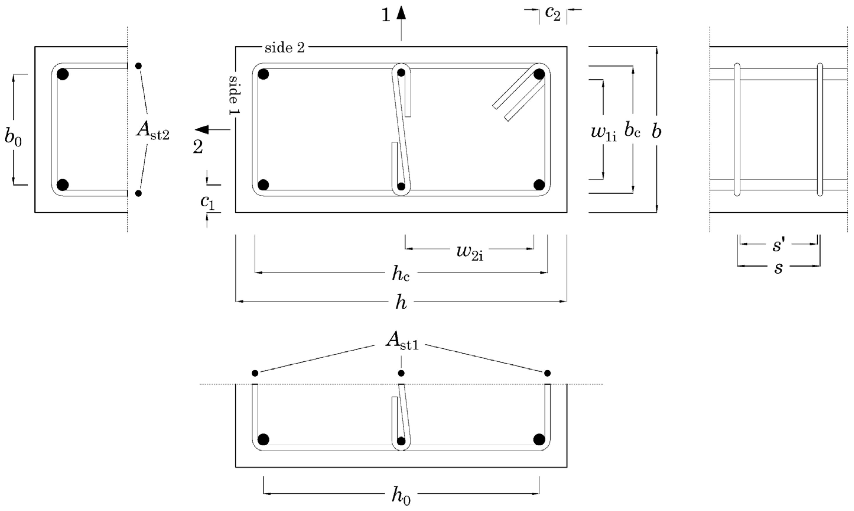
In this research study, the confinement mechanism is investigated with reference to prismatic elements characterized by a rectangular cross-section and endowed with stirrups and ties. Symbols adopted in this paper are shown in Figure 1. An orthogonal reference system is considered on the cross-section which identifies direction 1 (vertical direction in the figure) and direction 2 (horizontal direction in the figure). The maximum level of confinement may be calculated assuming that stirrups have yielded, and the lateral compressive stresses are uniformly distributed on the lateral surface of the concrete inside the center line of the stirrups. This situation corresponds to a confinement effect caused by stirrup legs with an extremely low spacing both in the cross-section and along the longitudinal axis of the member (later referred to as “uniform” confinement). The magnitude of this lateral compressive stress is, in general, different along the two orthogonal directions previously named 1 and 2. The lateral compressive stresses, σ_l1 and σ_l2, along such directions are given by the translation equilibrium between the lateral compressive force exerted by the transverse reinforcement on concrete and the axial force in the transverse reinforcement at yielding

$${\sigma }_{\mathrm{l}1}=\hspace{0.17em}{\mathsf{\rho }}_{\mathrm{st},1}\hspace{0.17em}{f}_{\mathrm{y},\mathrm{st}}$$

(5)

$${\sigma }_{\mathrm{l}2}=\hspace{0.17em}{\mathsf{\rho }}_{\mathrm{st},2}\hspace{0.17em}{f}_{\mathrm{y},\mathrm{st}}$$

(6)

where ρ_st,1 and ρ_st,2 are the volumetric ratio of the transverse reinforcement in the two orthogonal directions

$${\mathsf{\rho }}_{\mathrm{st},1}=\frac{{\displaystyle \sum _{i=1}^{n_{\mathrm{b},1}}{A}_{\mathrm{st},\mathrm{i}}\hspace{0.17em}}}{s\hspace{0.17em}{h}_{\mathrm{c}}}\hspace{1em}\hspace{1em}\hspace{1em}{\mathsf{\rho }}_{\mathrm{st},2}=\frac{{\displaystyle \sum _{i=1}^{n_{\mathrm{b},2}}{A}_{\mathrm{st},\mathrm{i}}\hspace{0.17em}}}{s\hspace{0.17em}{b}_{\mathrm{c}}}$$

(7)

In the above relations, n_b,1 and n_b,2 are the numbers of stirrups legs producing lateral compressive stresses in directions 1 and 2, respectively; A_st,i is the cross-sectional area of the single leg of the stirrup (or tie); b_c and h_c are the distances between the opposite legs of the stirrups, as reported in Figure 1.

4.1. Confinement Effectiveness Factor

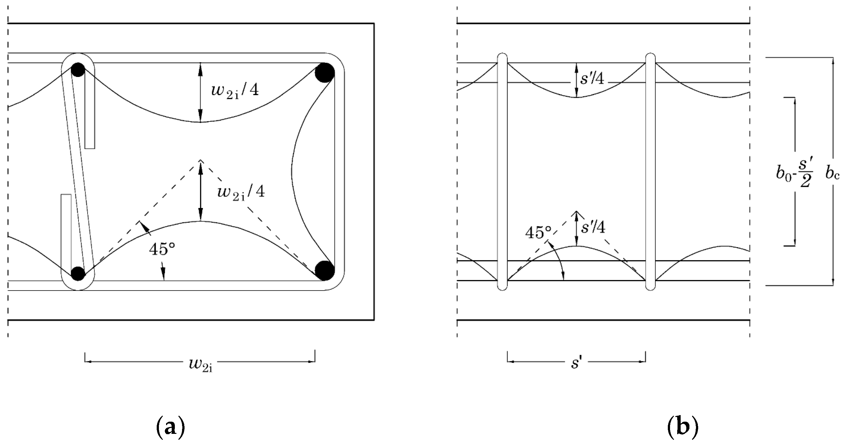
In the case of stirrups arranged with moderate or high spacing (s > 5 cm), the confinement effects are concentrated, in the plane of the transverse reinforcement, close to the longitudinal bars blocked to the transverse movement by stirrups or ties, as shown in Figure 2a. Starting from these blocked points the lateral confinement stresses spread towards the inside of the element, both in the plane of the transverse reinforcement and along the longitudinal axis of the member between two subsequent stirrups, as shown in Figure 2b. The three-dimensional spreading of the confinement stresses defines an effectively confined concrete volume that is smaller than the prismatic volume enclosed by the transverse reinforcement. The ratio between these two volumes provides an index of the effectiveness of confinement called “confinement effectiveness factor” (k_e). Applying this factor to the confinement stresses associated with a uniform confinement, the “effective” values of the confinement stresses are obtained.

$$f_{\mathrm{l}1}=k_{\mathrm{e}}\hspace{0.17em}{\mathsf{\rho }}_{\mathrm{st},1}\hspace{0.17em}{f}_{\mathrm{y},\mathrm{st}}$$

(8)

$$f_{\mathrm{l}2}=k_{\mathrm{e}}\hspace{0.17em}{\mathsf{\rho }}_{\mathrm{st},2}\hspace{0.17em}{f}_{\mathrm{y},\mathrm{st}}$$

(9)

To calculate k_e, the evaluation of the effectively confined volume is necessary. In the literature ([17,18,28]), it is commonly accepted that the lateral compressive stresses spread from the blocked points following parabolic arcs with ending tangents at 45° both in the plane of the cross-section and along the longitudinal axis of the member, as shown in Figure 2a,b. Even though a geometric description of the confined solid is possible, the rigorous calculation of its volume is not straightforward, particularly for complex arrangements of stirrups and ties. A conservative estimate of this volume is obtained by means of the approach introduced by Mander et al. [17] and currently adopted by standards, by means of two partial confinement effectiveness factors, named α_n and α_s, that embody the effects of confinement in the plane of the cross-section and along the longitudinal axis of the member.

The partial confinement effectiveness factor α_n is calculated in the plane of the cross-section and is the ratio of the area A_c,n that is effectively confined to the area enclosed by the center line of the stirrups. The factor α_s, instead, is calculated along the longitudinal axis of the member and is the ratio of the effectively confined area to the area enclosed by the center line of the longitudinal bars between two successive stirrups. The cross-sectional area of the effectively confined concrete A_e is obtained through the following relation as a function of both α_n and α_s, i.e.,

$$A_{\mathrm{e}}={\mathsf{\alpha }}_{\mathrm{n}}{\mathsf{\alpha }}_{\mathrm{s}}{A}_{\mathrm{c}}$$

(10)

where A_c is the cross-sectional area of concrete inside the center line of stirrups. The area A_e is considered constant along the longitudinal axis of the element (where spacing and layout of the stirrups are constant).

To evaluate α_n, let us consider the confinement stresses in the plane of the stirrups, i.e., where the effectively confined area is maximum and calculate the area A_c,n subtended by the parabolic arcs. If w_i is the inner distance between two adjacent bars blocked by stirrups, the area subtended by the single parabola is obtained through simple geometric considerations: a parabola with a tangent at 45° has a maximum height equal to w_i/4 and an average height equal to 2/3 of the maximum height. The area subtended by the single parabolic arc is therefore:

$$A_{\hspace{0.17em}\mathrm{p},\mathrm{i}}=\frac{1}{6}{w}_{\hspace{0.17em}\mathrm{i}}^{\hspace{0.17em}2}$$

(11)

The area A_c,n is obtained by subtracting the area subtended by the parabolic arcs from the area enclosed by the center line of the stirrups:

$$A_{\mathrm{c},\mathrm{n}}=b_{\mathrm{c}}{h}_{\mathrm{c}}-{\displaystyle \sum _{i=1}^{n_{\mathrm{b}1}-1}\hspace{0.17em}\frac{1}{6}{w}_{\hspace{0.17em}1,\mathrm{i}}^{\hspace{0.17em}2}}-{\displaystyle \sum _{i=1}^{n_{\mathrm{b}2}-1}\hspace{0.17em}\frac{1}{6}{w}_{\hspace{0.17em}2,\mathrm{i}}^{\hspace{0.17em}2}}$$

(12)

where w_1,i and w_2,i are the distances between adjacent blocked bars in the two directions.

The partial confinement effectiveness factor α_n is obtained dividing A_c,n by the area enclosed by the center line of the stirrups, i.e.,

$${\mathsf{\alpha }}_{\mathrm{n}}=1-{\displaystyle \sum _{i=1}^{n_{\mathrm{b}1}-1}\hspace{0.17em}\frac{1}{6\hspace{0.17em}{b}_{\mathrm{c}}{h}_{\mathrm{c}}}{w}_{\hspace{0.17em}1,\mathrm{i}}^{\hspace{0.17em}2}}-{\displaystyle \sum _{i=1}^{n_{\mathrm{b}2}-1}\hspace{0.17em}\frac{1}{6\hspace{0.17em}{b}_{\mathrm{c}}{h}_{\mathrm{c}}}{w}_{\hspace{0.17em}2,\mathrm{i}}^{\hspace{0.17em}2}}$$

(13)

To evaluate α_s, let us consider the parabolic arcs between two subsequent stirrups in the direction of the longitudinal axis. At a distance s′/2 from the stirrups, where s′ is the inner distance between two successive stirrups, the confined area reduces to the value given by the following relation

$$A_{\mathrm{c},\mathrm{s}}=\left(b_{\mathrm{c}}-\frac{s^{\prime }}{2}\right)\left(h_{\mathrm{c}}-\frac{s^{\prime }}{2}\right)=b_{\mathrm{c}}{h}_{\mathrm{c}}\left(1-\frac{s^{\prime }}{2\hspace{0.17em}{b}_{\mathrm{c}}}\right)\left(1-\frac{s^{\prime }}{2\hspace{0.17em}{h}_{\mathrm{c}}}\right)$$

(14)

Dividing the area A_c,s by the area enclosed by the centerline of the stirrups, the partial confinement effectiveness factor α_s is obtained:

$${\mathsf{\alpha }}_{\mathrm{s}}=\left(1-\frac{s^{\prime }}{2\hspace{0.17em}{b}_{\mathrm{c}}}\right)\left(1-\frac{s^{\prime }}{2\hspace{0.17em}{h}_{\mathrm{c}}}\right)$$

(15)

This expression is the one proposed by Chang and Mander [18]. A similar expression is reported in Eurocode 8 [29], where, however, the distances w_i and s′ are measured from the centroid of the bars and from the centerline of the stirrups, respectively.

4.2. Proposed Volume of Confined Concrete

The procedure set out in the previous section brings the effectively confined volume, defined in three dimensions by the spreading of the confinement stresses, back to a prismatic volume having cross-sectional area A_e, as described in Equation (10). To investigate the effects of the simplifications reported in Eurocode 8 for the evaluation of this latter cross-sectional area, Vulinovic et al. [30] have recently calculated the exact value of the above effectively confined concrete volume starting from the geometrical assumptions of Eurocode 8, i.e., assuming that the ends of the parabolic arcs are inclined at an angle of 45°. The rigorous calculation was performed graphically by means of the software Autocad. In particular, the external surface of the effectively confined volume was obtained by translating the parabolic arcs that lie on a cross-section along the longitudinal axis of the member on the parabolic arcs that go from one stirrup to another. The resulting volume obtained by the rigorous calculation was assumed to be the “exact” volume of the effectively confined concrete. Then, the “exact” confinement effectiveness factor was calculated as the ratio of the exact volume of the effectively confined concrete to the volume of the concrete inside the center lines of the stirrups. This exact value of the confinement effectiveness factor was compared with the value of the confinement effectiveness factor calculated according to Eurocode 8. The investigation was conducted on a series of columns with square cross-section characterized by different arrangements of the transverse reinforcement.

The results showed that, in all the considered cases, the analytical evaluation performed according to EC8 led to conservative evaluations of the confinement effectiveness factor, i.e., the value of the confinement effectiveness factor determined by EC8 was always lower than the geometrically rigorous confinement effectiveness factor. Specifically, the “exact” confinement effectiveness factor was, on the average, 32% higher than the factor evaluated according to EC8. This proved that the simplifications that are usually introduced for the evaluation of the confinement effectiveness factor led to a significant underestimation of this factor.

In addition to these observations, it is important to keep in mind that the confinement mechanism is based on the hypothesis that the confinement stresses spread towards the interior of the member following parabolic arcs with tangents at 45°. To the knowledge of the authors, this assumption was introduced by Sheikh and Uzumeri [28] without any supporting experimental justification. In light of these considerations, the evaluation of the confinement effectiveness factor with the method based on factors α_n and α_s described above appears to be rather penalizing. In line with these conclusions, Ghersi [31] suggested reducing the subtractive terms of the factor α_n by 2/3 and thus proposed the following relation:

$${{\mathsf{\alpha }}^{\prime }}_{\mathrm{s}}=\left(1-\frac{s^{\prime }}{3\hspace{0.17em}{b}_{\mathrm{c}}}\right)\left(1-\frac{s^{\prime }}{3\hspace{0.17em}{h}_{\mathrm{c}}}\right)$$

(16)

It should be noted that the calculation of the confinement effectiveness factor shown above refers to the case of members subjected to axial force only and thus to members not in a seismic condition. In fact, in the occurrence of earthquakes, columns are always subjected to the combined action of axial force and bending moment and often are cracked because of these internal forces. Beams can even be cracked because of the action of the sole effect of gravity loads. In any case, cracking causes confinement conditions that are different from those in uniformly compressed members. However, in the conventional analysis of structures the confinement effectiveness factor remains equal to the one determined assuming that the section is entirely and uniformly compressed.

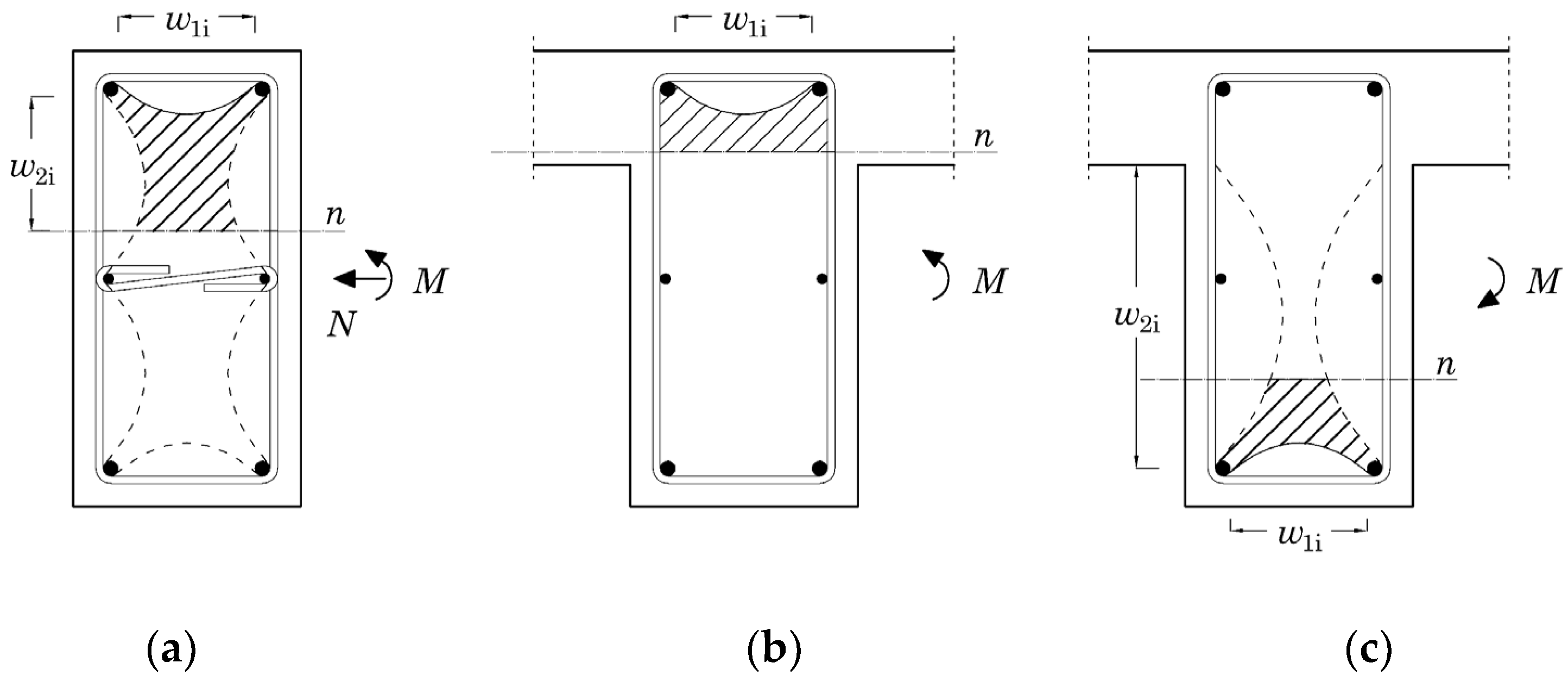
More specifically, close to the neutral axis of the cross-section, concrete subjected to low positive strains offers an efficient confinement to the adjacent compressed material, as shown in Figure 3a. This is valid for both columns and beams. Beams, however, deserve a separate comment owing to their partial embedment in the slab. In fact, if the beam is subjected to positive bending moment and the compressed part of the cross-section falls within the depth of the slab, the concrete in the compressed part of the beam cross-section is confined by the slab. In such cases, a less effective confinement action can occur only on the upper side of the member, as shown in Figure 3b [31]. If the bending moment is negative, the concrete subjected to low positive longitudinal strains provides an efficient confinement at the level of the neutral axis; on the remaining sides of the cross-section the confinement effectiveness is governed by the presence of longitudinal bars that are blocked to the lateral movement by stirrups and ties. However, the parabolic arcs on the left and right sides of the beam extend from the longitudinal bars in compression to the intrados of the slab, and not from the longitudinal bars in compression to the longitudinal bars in tension. This determines a lower height of the parabolic arcs that develop on the left and right sides of the cross-section, as shown in Figure 3c [31]. Referring to the case of columns, the authors note that the simulation of the response of the specimens on the basis of the confinement effectiveness factors calculated according to Eurocode 8 has revealed the impossibility to reproduce with satisfying accuracy the response of some members, particularly of those with low values of the volumetric ratio of the transverse reinforcement, owing to the low values of the corresponding confinement effectiveness factors.

Based on the above considerations and to the evidence of the numerical simulations, the authors propose here to use (for members subjected to combined axial force and moderate-to-large bending moments) a diffusion angle of the confinement stresses lower than 45° and such as to reduce the height of the parabolic arcs by 50%, compared with the case with a tangent at 45° (the proposed angle is equal to 26.57°). This means considering a similar reduction for the subtractive terms that appear in the expressions of the coefficients α_n and α_s, i.e.,

$${\mathsf{\alpha }}_{\mathrm{n}}=1-0.5{\displaystyle \sum _{i=1}^{n_{\mathrm{b}1}-1}\hspace{0.17em}\frac{1}{6\hspace{0.17em}{b}_{\mathrm{c}}{h}_{\mathrm{c}}}{w}_{\hspace{0.17em}1,\mathrm{i}}^{\hspace{0.17em}2}}-0.5\hspace{0.17em}{\displaystyle \sum _{i=1}^{n_{\mathrm{b}2}-1}\frac{1}{6\hspace{0.17em}{b}_{\mathrm{c}}{h}_{\mathrm{c}}}{w}_{\hspace{0.17em}2,\mathrm{i}}^{\hspace{0.17em}2}}$$

(17)

$${\mathsf{\alpha }}_{\mathrm{s}}=\left(1-0.5\frac{s^{\prime }}{2\hspace{0.17em}{b}_{\mathrm{c}}}\right)\left(1-0.5\frac{s^{\prime }}{2\hspace{0.17em}{h}_{\mathrm{c}}}\right)$$

(18)

4.3. Application of Confinement to the Numerical Model

According to the approach proposed by Mander et al. [17], the properties of the unconfined concrete are assigned to the concrete fibers that fall outside the center line of the outermost stirrups, whereas those determined through the confinement model by means of the effective confinement stresses [Equations (8) and (9)] are assigned to the fibers inside the center line of the outermost stirrups. Thereby, the confinement effectiveness coefficient affects the strength and ductility properties of the entire prismatic volume of concrete inside the center line of the outermost stirrups.

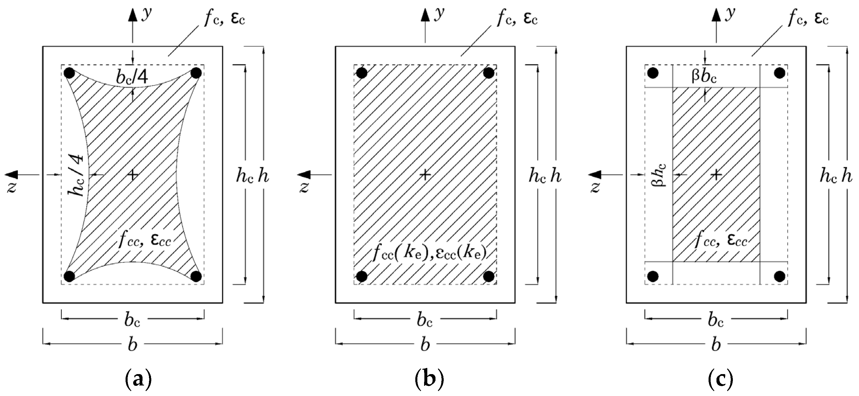
To arrive at a simpler and more accurate description of the confinement mechanism in the column, the authors propose here to apply the mechanical properties of the “uniformly” confined concrete to a part of the concrete fibers that are inside the center line of the outermost stirrups and that are characterized by a total area equal to A_e [see Equation (10)]. This approach is consistent with the geometric meaning of the confinement effectiveness factor.

Virtually, it would be possible to discretize the cross-section so as to reproduce the spreading of the confinement stresses in the cross-section (Figure 4a). However, as resulting from the numerical analyses, such a level of detail is not advantageous, also because of the inevitable complications in the description of the concrete patches. The solution suggested herein envisages the search for a rectangular perimeter of the “uniformly” confined concrete which is obtained through an offset of the center line of the outermost stirrups (Figure 4b,c). The distance from the proposed perimeter to the center line of the outermost stirrups is defined as a function of a scale factor β and of the lengths b_c and h_c, as shown in Figure 4c. The scale factor is obtained equating the area of the new rectangular patch of confined concrete to the area of the rectangle defined by the center lines of the outermost stirrups times the effectiveness confinement factor, i.e.,

$$b_{\mathrm{c}}{h}_{\mathrm{c}}-2\mathsf{\beta }{b}_{\mathrm{c}}^2-2\mathsf{\beta }{h}_{\mathrm{c}}^2+4{\mathsf{\beta }}^2{b}_{\mathrm{c}}{h}_{\mathrm{c}}=k_{\mathrm{e}}{b}_{\mathrm{c}}{h}_{\mathrm{c}}$$

(19)

Reordering and solving the above equation for β leads to the following relation:

$$\mathsf{\beta }=\frac{2\left(b_{\mathrm{c}}^2+h_{\mathrm{c}}^2\right)\pm \sqrt{4{\left(b_{\mathrm{c}}^2+h_{\mathrm{c}}^2\right)}^2-16\hspace{0.17em}{b}_{\mathrm{c}}^2{h}_{\mathrm{c}}^2\hspace{0.17em}\left(1-k_{\mathrm{e}}\right)}}{8\hspace{0.17em}{b}_{\mathrm{c}}{h}_{\mathrm{c}}}$$

(20)

The sign corresponding to the desired solution is the one for which, if k_e = 1, the β scale factor is equal to 0, i.e., the minus sign.

5. Modeling of Members

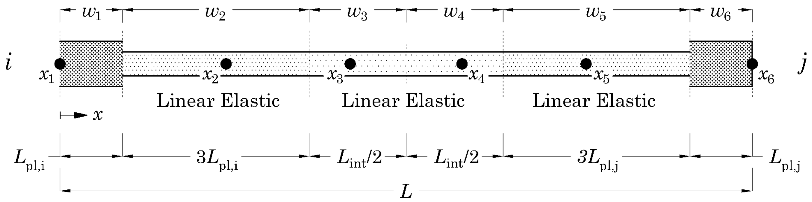
In this research study, the authors have used the forceBeamColumn element implemented in OpenSees with the “HingeRadau” integration rule. The choice of using a model with concentrated plasticity instead of distributed plasticity is justified by the following reasons: (1) In general, in the study of framed buildings in seismic situations, the formation of plastic hinges is expected at the ends of members and is rare in the middle of a member (e.g., beam) and (2) the adoption of a simpler model of a member implies greater computational effectiveness, which translates into a greater numerical stability of the model and higher processing rate.

The formulation of the element used for the analyses was proposed by Scott and Fenves [32] (Modified Two-Point Gauss Radau) and considers a total of six integration points: while the first and last points fall into the inelastic parts at the ends of the element, the other four points fall into the central elastic section, as shown in Figure 5. The ending sections have length equal to L_pl,i and L_pl,j. The elastic section is further divided into three sub-sections of lengths equal to 3L_pl,i, L-4(L_pl,i+ L_pl,j), and 3L_pl,j, respectively. The weights corresponding to the integration points 1 and 6 (x₁ = 0, x₆ = L) are equal to L_pl,i and L_pl,j, whereas the weights corresponding to points 2 and 5 (x₂ = 8/3 L_pl,i, x₅ = L-8/3 L_pl,j) are equal to 3L_pl,i and 3L_pl,j, respectively.

The formulation above was preferred to others since it allows the user to govern the localization of damage in the plastic hinge region by simply adjusting the values of L_pl,i and L_pl,j.

For more details on the formulation of the considered forceBeamColumn element, the readers are invited to refer to reference [32], as an exhaustive discussion of the subject is beyond the scope of this work.

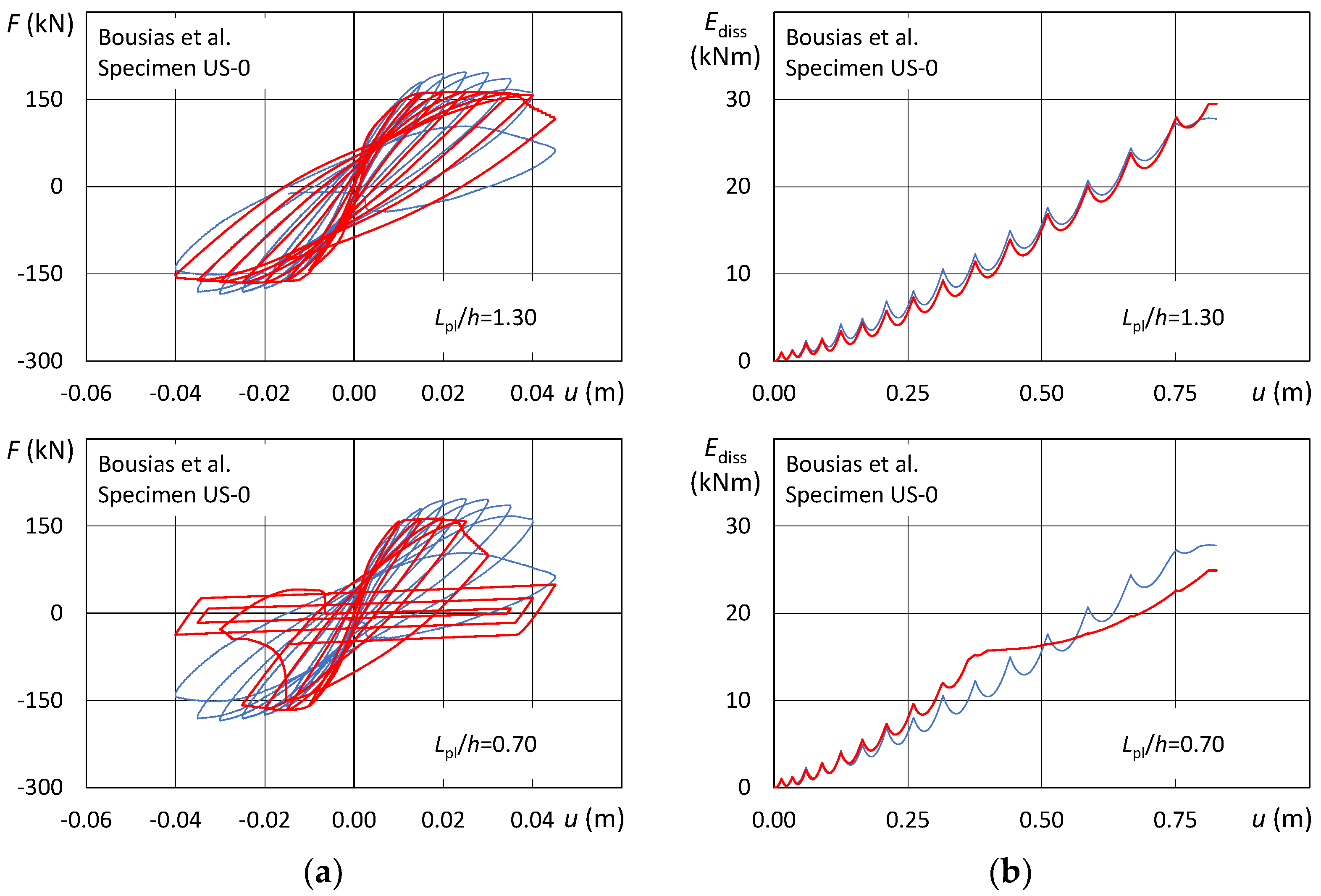
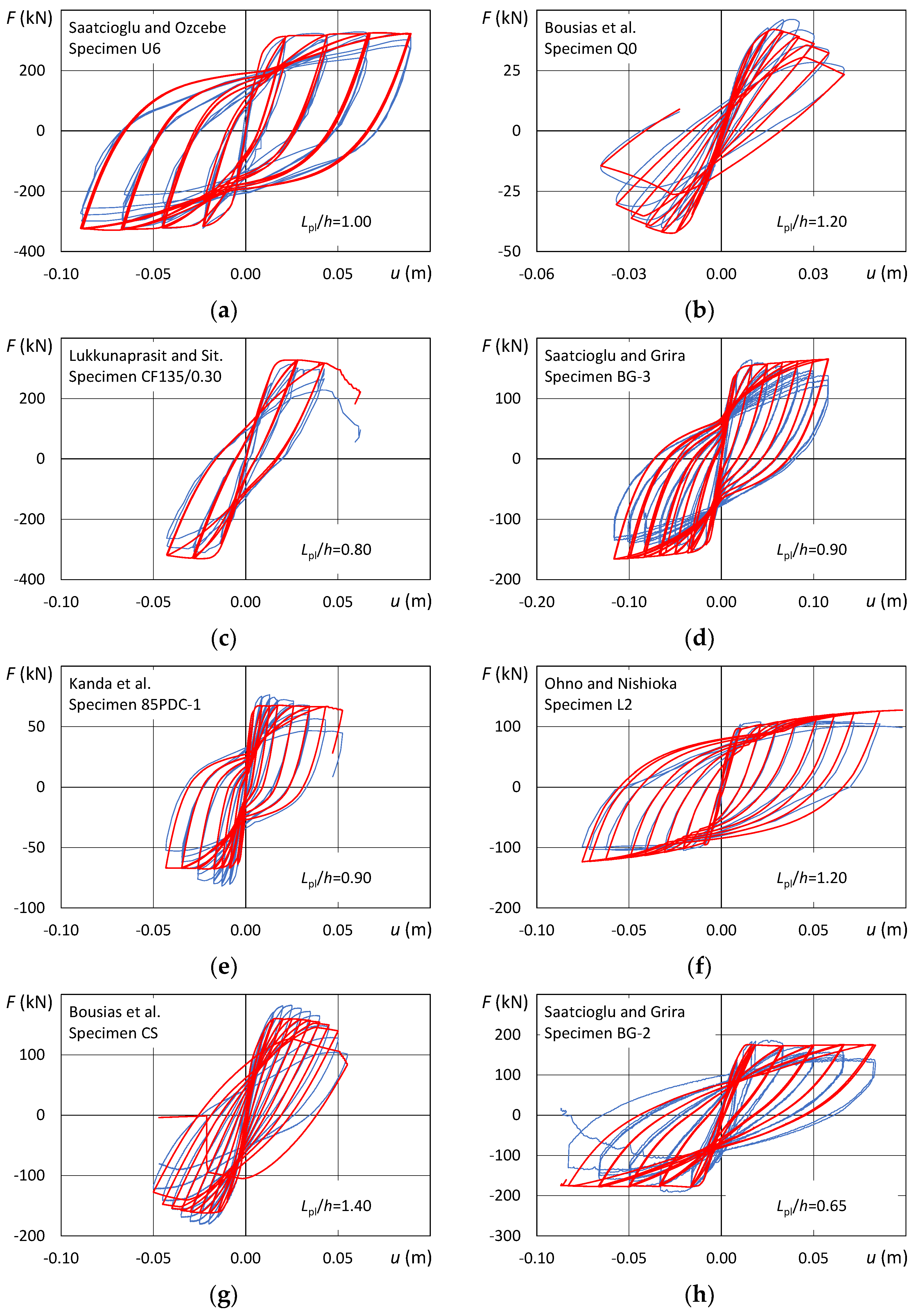
6. Laboratory Tests

The considered laboratory tests have been selected from the database of the European Union Seventh Framework Program [FP7/2007-2013] [33]. This database contains data on hundreds of experiments divided by type of RC element (beams, columns and walls). The available information includes (1) geometry of the cross-section, (2) size of the specimen and configuration of the test setup, (3) cross-sectional area and arrangement of the longitudinal and transverse reinforcements, (4) axial force, (5) mechanical properties of concrete and steel, and (6) cyclic force-displacement data recorded during the laboratory test.

The selected specimens are representative of RC columns that are common in existing buildings built between the 1970s and early 2000s. In particular, the authors have selected tests conducted on columns (i.e., members with axial force and symmetric longitudinal reinforcement) with a rectangular cross-section and failing in a flexural mode without slippage of the steel bars. Some other filters were placed (with a few exceptions) on material properties, loading conditions, and geometry. In particular, the compressive strength of concrete f_c is in the range from 18 to 48 MPa, the yielding strength of the longitudinal bars f_yl is in the range from 313 to 586 MPa, the shear span ratio L_v/h is in the range from 3 to 7.6; the diameter of the bars is in the range from 14 mm to 20 mm and the normalized axial force ν is in the range from 0 to 0.77.

As a result, a total of 33 tests were selected from the following research: Bousias et al. [34,35], Saatcioglu and Ozcebe [36], Saatcioglu and Grira [37], Sheikh and Khoury [38], Kanda et al. [39], Ohno and Nishioka [40], Lukkunaprasit and Sittipunt [41], and Matamoros [42].

Table 1. Main geometric and mechanical characteristics of the selected specimens.

	ID	fc [MPa]	fyl [MPa]	B [mm]	H [mm]	Lv/d [-]	ρs,tot [%]	ρvol,st [%]	N/Acfc [-]
Bousias et al. [34,35]	US-0	18.30	560	250	500	3.42	0.81	0.40	0.38
Bousias et al. [34,35]	CS-0	18.30	560	250	500	3.42	0.81	0.40	0.38
Bousias et al. [34,35]	Q-0	27.00	313	250	250	7.62	0.99	0.52	0.44
Bousias et al. [34,35]	Q-0L1	30.30	313	250	250	7.27	0.99	0.47	0.41
Bousias et al. [34,35]	Q-0L2	30.30	313	250	250	7.27	0.99	0.47	0.42
Bousias et al. [34,35]	Q-0L1a	28.10	313	250	250	7.27	0.99	0.47	0.63
Bousias et al. [34,35]	Q-0L2a	28.10	313	250	250	7.27	0.99	0.47	0.57
Bousias et al. [34,35]	Q-RCM	30.60	487	400	400	4.57	0.79	0.95	0.18
Saatcioglu and Grira [37]	BG-1	34.00	456	350	350	5.45	1.95	0.99	0.43
Saatcioglu and Grira [37]	BG-2	34.00	456	350	350	5.45	1.95	1.98	0.43
Saatcioglu and Grira [37]	BG-3	34.00	456	350	350	5.45	1.95	1.97	0.20
Saatcioglu and Grira [37]	BG-4	34.00	456	350	350	5.45	2.93	1.31	0.46
Saatcioglu and Grira [37]	BG-5	34.00	456	350	350	5.45	2.93	2.66	0.46
Saatcioglu and Grira [37]	BG-6	34.00	478	350	350	5.55	2.29	2.64	0.46
Saatcioglu and Grira [37]	BG-7	34.00	456	350	350	5.40	2.93	1.27	0.46
Saatcioglu and Grira [37]	BG-8	34.00	456	350	350	5.40	2.93	1.28	0.23
Saatcioglu and Grira [37]	BG-10	34.00	428	350	350	5.42	3.28	2.64	0.46
Sheikh and Khoury [38]	AS 18	32.80	508	305	305	6.82	2.45	2.64	0.77
Sheikh and Khoury [38]	AS 19	32.30	508	305	305	6.82	2.45	1.49	0.47
Sheikh and Khoury [38]	AS 3	33.20	508	305	305	6.82	2.45	1.49	0.60
Sheikh and Khoury [38]	ES 13	32.60	508	305	305	6.82	2.45	1.67	0.76
Kanda et al. [39]	85PDC-1	24.80	374	250	250	3.69	1.62	1.09	0.12
Ohno and Nishioka [40]	L1	24.80	362	400	400	4.57	1.42	0.78	0.03
Ohno and Nishioka [40]	L2	24.80	362	400	400	4.57	1.42	0.78	0.03
Ohno and Nishioka [40]	L3	24.80	362	400	400	4.57	1.42	0.78	0.03
Lukkunaprasit and Sittipunt [41]	CF135/0.30	35.70	471	400	400	4.16	3.14	0.91	0.30
Lukkunaprasit and Sittipunt [41]	CF135/0.37	30.50	475	400	400	4.16	3.14	0.91	0.37
Matamoros [42]	C5-20N	48.30	586	203	203	4.14	1.93	3.04	0.14
Matamoros [42]	C5-40N	38.10	572	203	203	3.70	1.93	2.40	0.36
Saatcioglu and Ozcebe [36]	U3	34.80	430	350	350	3.28	3.21	1.42	0.14
Saatcioglu and Ozcebe [36]	U4	32.00	438	350	350	3.28	3.21	2.13	0.15
Saatcioglu and Ozcebe [36]	U6	37.00	437	350	350	3.28	3.21	1.02	0.13
Saatcioglu and Ozcebe [36]	U7	39.00	437	350	350	3.28	3.21	1.02	0.13

summarizes the tests selected together with the main geometric and mechanical characteristics of the specimens, including the geometric percentage of the volumetric ratio of the transverse reinforcement ρ_vol,_st and the geometric ratio of the longitudinal reinforcement ρ_s,tot.

7. Numerical Analyses

Each specimen is modeled as a 2D cantilever beam with a rotational spring at the base. This latter component is added to reproduce the elastic rotational deformability at the base of the specimen. The three degree of freedom numerical model consists of three nodes connected by two elements i.e., one forceBeamColumn element and one zero-length element. Nodes 1 and 2 have coordinates that coincide with the origin of the reference system and node 3 has the abscissa equal to that of the nodes 1 and 2 and the ordinate equal to the height of the specimen, measured from the base to the point of application of the lateral force. All the degrees of freedom of node 1 are restrained. The zero-length element connects nodes 1 and 2 while the forceBeamColumn element connects nodes 2 and 3. The assigned zero-length element consists of three elastic springs. The stiffness of the material assigned to the rotational spring is calibrated so that the slope of the initial part of the simulated response matches the slope of the first part of the experimental response; the stiffness of the elastic material assigned to the translational springs is very high to prevent relative displacements between nodes 1 and 2. The value of the length of the plastic hinge to be assigned to the fixed end of the forceBeamColumn element is calibrated to match the response of the laboratory test. At the other end of the element a very small value is assigned to le plastic hinge length (i.e., 1.0 cm). Both the inelastic and elastic sections of the element are assigned a discretized fiber cross-section according to the criteria set out in previous sections. Three materials are assigned to the fibers of the inelastic section: two concrete materials (one for confined material and one for non-confined material) and one steel material. The considered uniaxial material models are “Concrete04” and “ReinforcingSteel”. The mechanical properties assigned to the materials in the inelastic sections of the element have been discussed in previous sections. The concrete material model assigned to the relevant fibers of the elastic section is characterized by the elastic modulus of the unconfined concrete whereas the steel material model is characterized by the elastic modulus of steel. Second order effects are not simulated as they had been eliminated from the results of the laboratory tests [33].

The axial force is first applied to node 3 through a force control integration procedure. Then, the cyclic test is reproduced by applying a displacement protocol at Node 3 in the transverse direction, via a displacement control integration procedure. The displacement story of the test that is to be reproduced is used as displacement protocol. The Krylov-Newton integration algorithm is used. The “Norm Unbalance” test with tolerance set equal to 5 × 10⁻³ is used to determine if convergence has been reached or not.

8. Optimal Length of the Plastic Hinge

The only data of the model that need to be calibrated are the stiffness of the rotational spring at the base of the element and the length of the plastic hinge. The stiffness of the rotational spring is first adjusted to match the stiffness of the specimen in the initial phase of the laboratory test. Then, the length of the plastic hinge L_pl is modified until a correspondence between the real and simulated responses is obtained.

The accuracy of the numerical simulation is preliminarily evaluated by comparing the visual aspect of the lateral force-lateral displacement plots. Subsequently, the accuracy in the prediction of the cumulated energy dissipated at each cycle of the loading protocol has been determined by comparing the cumulated area subtended by the above plots. As an example, the comparison between the laboratory test and numerical responses is reported in Figure 6 for two values of length of plastic hinge (L_pl/h = 1.30 or 0.70) with reference to the specimen US-0 tested by Bousias et al. [34]. In particular, the lateral load-lateral displacement plots are reported on the left side of the figure while the energy cumulated-lateral displacement plot is on the right side of the figure. The curve referring to the laboratory test is shown by solid blue line while the curve referring to the numerical test is shown by solid red line. As is evident, an erroneous evaluation of the length of the plastic hinge (in this case 0.70) may cause significantly inaccurate evaluations of the flexural response. In particular, the underestimation of the length of the plastic hinge causes higher strains in the plastic hinge, and thus leads to overestimate severely the degradation of the mechanical strength and stiffness of the column.

The lateral load, lateral displacement plots referring to some of the considered specimens and to the numerical analyses performed with the optimal length of the plastic hinge are illustrated in Figure 7. The numerical simulation of the real tests highlights the effectiveness of the modeling and the numerical stability of the model. In general, once the length of the plastic hinge has been given a proper value, the numerical model reveals the ability to accurately simulate the hysteretic cycles of the experimental tests regardless of the geometric, mechanical, and construction details of the single test. It should also be noted that the laboratory tests were pushed up to displacements associated with chord rotation demands much greater than the corresponding ultimate values. Even in these conditions, the proposed numerical models showed no signs of numerical instability.

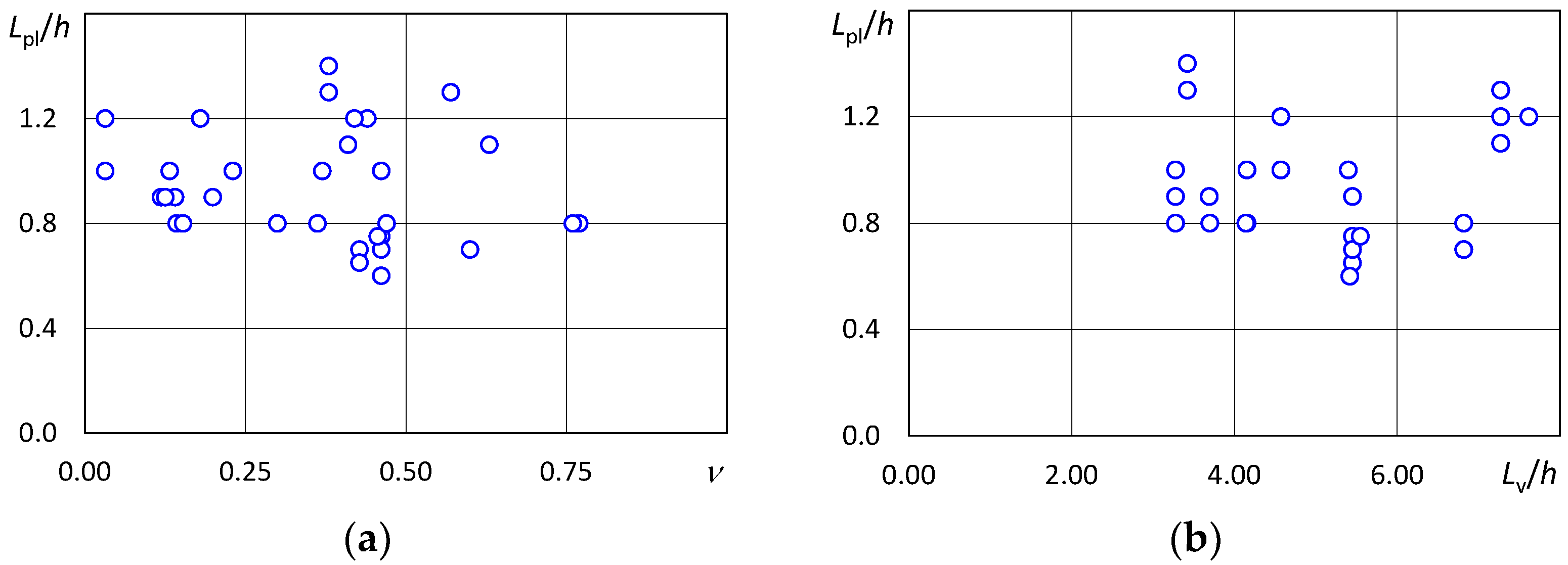
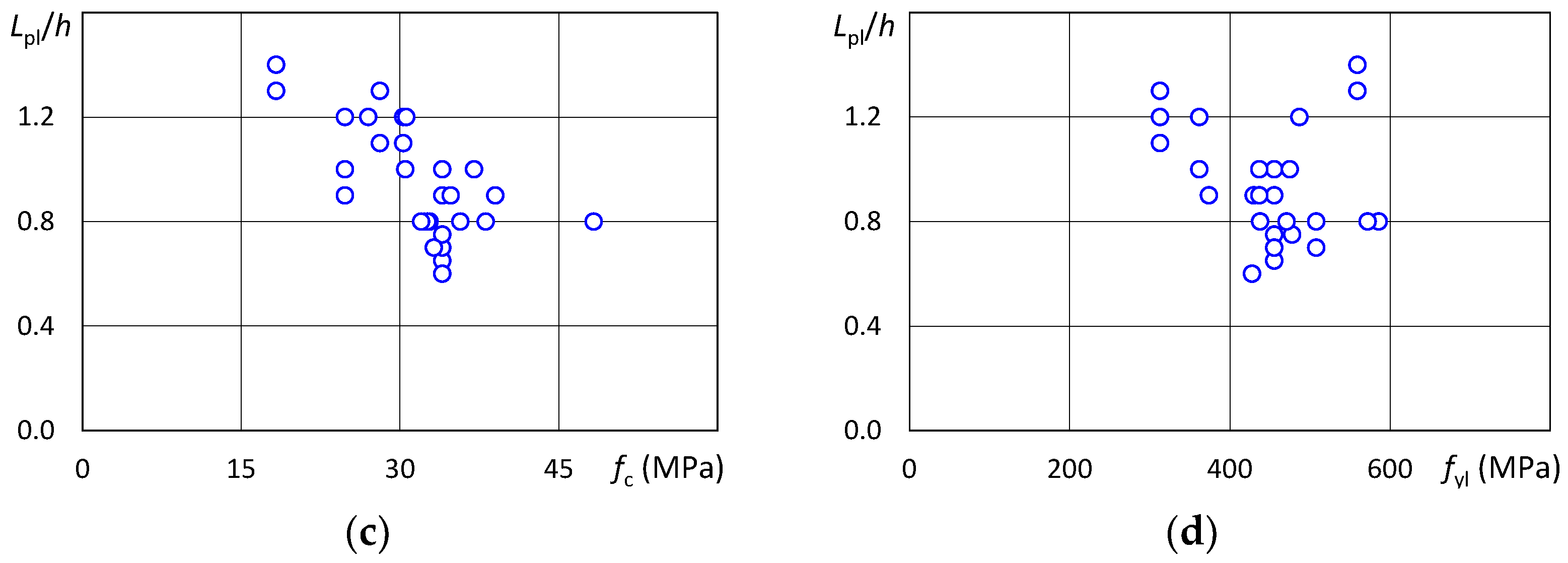
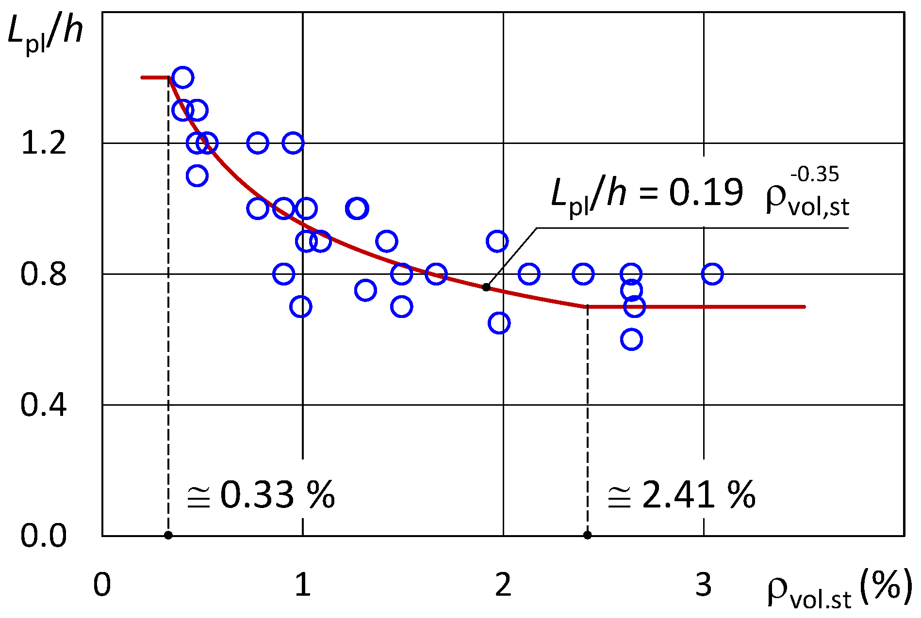
9. Proposed Expression of the Length of the Plastic Hinge

To propose a relation for the determination of the length of the plastic hinge, the values of L_pl obtained through calibration have been plotted as a function of the main geometric and mechanical parameters of the specimens. First, the dependence of L_pl on the normalized axial force ν has been investigated. Among the selected tests, the values of ν (0.0 ÷ 0.77) vary in a wide range of values and this should be sufficient to identify any possible dependence of L_pl on ν. However, the plot of the normalized length of the plastic hinge L_pl/h versus ν, reported in Figure 8a, does not show a clear trend. Equally dispersed are also the points that represent L_pl/h as a function of the shear span ratio L_V/h of the specimen, as shown in Figure 8b. The trend of L_pl/h as a function of the compressive strength of the concrete f_c seems to reveal an inverse proportionality relationship, as shown in Figure 8c. However, the authors of the present paper believe that the values of the compressive strength considered here, with a single exception, vary in a narrow range (i.e., 18-40 MPa) and do not allow general and reliable conclusions. On the other hand, for the considered specimens, L_pl/h does not show any appreciable trend as a function of the yield strength of the longitudinal steel bars f_yl, as shown in Figure 8d. Finally, the optimal length of the plastic hinge L_pl/h is represented as a function of ρ_vol,st by blue circles in Figure 9. In this case, an inverse proportionality relationship is evident between L_pl/h and ρ_vol,st. In particular, for values of ρ_vol,st between 0.50% and 1.50%, the value of L_pl/h varies from a maximum value of about 1.50 up to about 0.70. The value of L_pl/h remains almost constant for ρ_vol,st greater than 2.00%. This trend is effectively interpreted through a power function of the type:

$$L_{\mathrm{pl}}/h=a\hspace{0.17em}{\mathsf{\rho }}_{\mathrm{vol},\mathrm{st}}^{\mathrm{b}}+c$$

(21)

where the values of the coefficients a, b and c have been obtained through an optimization procedure performed using the Excel Solver. Specifically, starting from tentative values of a, b, and c, the optimization procedure searches for a combination of the three coefficients which minimizes the sum of the squares of the differences between the optimal values of L_pl/h and the predicted values. In order to consider more mathematical solutions, the optimization procedure has been repeated 20 times with different tentative values. Based on the values of a, b, and c giving the optimal solutions, the following formula is proposed:

$$L_{\mathrm{pl}}/h=0.19\hspace{0.17em}{\mathsf{\rho }}_{\mathrm{vol},\mathrm{st}}^{-0.35}$$

(22)

Coefficient “c” resulting from the optimization process was always negligible and then has been assumed equal to zero in the proposed equation. Further, it has been chosen to limit the proposed value of L_pl/h to 1.40 from above and to 0.70 from below. These limitations come into play for values of ρ_vol,st lower than 0.33% and greater than 2.41%, respectively. Figure 9 shows the prediction of the optimal values of L_pl/h in the range of values of ρ_vol,st of practical interest.

10. Conclusions

This paper deals with the problem of numerical modeling of members of existing reinforced concrete buildings and specifically with two crucial aspects in modeling of reinforced concrete members: (1) the application of the confinement model to RC members and (2) the calibration of the length of the plastic hinge. Both issues have been treated to achieve accuracy of response, numerical stability, and computational efficiency.

The proposed numerical model uses the element with concentrated plasticity proposed by Scott and Fenves [32]. The uniaxial material model considered for concrete is named “Concrete04” in Opensees whereas the uniaxial material model considered for the longitudinal bars is named “ReinforcingSteel”.

The value of the plastic hinge length that leads to the best prediction of the cyclic response of laboratory tests available in the literature has been determined. The examined specimens are representative of reinforced concrete columns of existing buildings built between the 1970s and early 2000s. In particular, the authors have selected tests conducted on columns with rectangular cross-section and failing in a flexural mode without slipping of steel bars. In most cases, the shear span ratio of the specimens is in the range from 3 to 6 and the normalized axial force is in the range from 0.2 to 0.4. The average compressive strength of concrete is in the range from 20 to 40 MPa and the yielding strength of the longitudinal bars is in the range from 350 to 500 MPa.

The main conclusions of the study are here reported:

-

The confinement effectiveness factor calculated according to Eurocode 8 penalizes the response of RC columns, particularly those with low values of the volumetric ratio of the transverse reinforcement. The authors have proposed a less restrictive volume of confined concrete, in addition to a fiber discretization technique that is consistent with the geometric meaning of the confinement effectiveness factor.

-

A simple relation has been proposed to calculate the optimum length of the plastic hinge of the numerical element with concentrated plasticity. The optimum length of the plastic hinge decreases with the increase of the volumetric ratio of the transverse reinforcement and ranges from 0.7 to 1.4 times the depth of the cross-section.

The conclusions are drawn based on a set of specimens with moderate variation of the geometric and mechanical properties of the materials in order to represent the response of usual members of existing reinforced concrete buildings. A greater number of laboratory tests will be considered in the future to extend the proposed modeling to a broader range of the considered parameters.