1. Introduction
Buildings consume most of their energy during the operating phase of their entire service life. Specifically, about 60% of energy is used for air conditioning to provide a comfortable living and working environment [
1,
2,
3]. In order to reduce energy consumption in buildings, efficient energy use and management should be implemented for the operational phase. To meet this need, countless studies have been undertaken that focus on the development of high-efficiency facilities, control solutions, and energy management systems. However, in order to optimize energy performance from the design stage to the operation stage, the accurate prediction of energy consumption and the demands of the building must be addressed first.
Various studies of accurate energy consumption and demand prediction have employed neural network techniques based on machine learning. For example, Cheng et al. used an artificial neural network (ANN) model to investigate building envelope performance, parameters, heating degree day, and cooling degree day as input variables and were able to increase the prediction accuracy by more than 96% compared to the existing method [
4].
Peng et al. proposed an ANN model that predicts the refrigeration load by combining the box model and Jenkins model and showed performance of less than 2.1% mean absolute percentage error [
5]. Roldan et al. proposed an ANN model for predicting the time-temperature curve using short-term building energy consumption, usage temperature, and type of building as input variables. They obtained high prediction accuracy after testing in real buildings for one year [
6].
Turhan et al. compared the results of predicting the thermal load according to the building envelope conditions using ANN with those obtained from the building energy simulation tool. They observed a high similarity between ANN prediction techniques and the results of building energy simulation tools and confirmed an average absolute percentage of 5.06% and a prediction success rate of 0.977 [
7]. Ferlito et al. developed an ANN model that uses monthly building electrical energy consumption data and showed a prediction accuracy of 15.7% to 17.97% root mean square error (RMSE) [
8]. Li et al. proposed an energy consumption prediction technique that simplifies a complex building into several blocks in the initial design stage based on an ANN algorithm. The prediction result of cooling and heating energy consumption showed a relative deviation within ±10%, and the total energy consumption showed a predictive performance within 10% of the relative deviation [
9].
Le Cam et al. used a closed-loop nonlinear autoregressive neural network training algorithm to predict the energy consumption of the air supply fan in an air-handling unit (AHU) [
10]. Their results showed a predictive performance of 5.5% RMSE and 17.6% coefficient of variation of the RMSE (CvRMSE) [
10]. Ahmed et al. predicted the power load of a single building using ANN and random forest (RF) models and compared and analyzed each predictive performance. Their proposed ANN model yielded an average CvRMSE of 4.91%, and the RF model showed an average CvRMSE of 6.10% by adjusting the depth of the tree [
11].
Ding et al. investigated prediction accuracy by combining eight input variables using an ANN model and a support vector machine (SVM) [
12]. They improved the prediction accuracy by optimizing the combination of variables using K-means, and among the variables, historical cooling capacity data showed the highest correlation with prediction accuracy [
12].
Koschwitz et al. predicted data-driven thermal loads using NARX RNNs (nonlinear autoregressive exogenous recurrent neural networks) of different depths and an ε-SVM regression model. Predicting the monthly load in non-residential regions in Germany found that the NARX RNNs showed higher accuracy levels than the ε-SVM regression model [
13]. Niu et al. evaluated the energy consumption prediction performance of the AHU in a Bayesian network training model and ARX (autoregressive with external) model. All the models used in their study satisfied ASHRAE Guideline 14 and, among them, the Bayesian network training algorithm exhibited the best prediction performance [
14]. Chen et al. improved the accuracy of the prediction model by adopting the concept of clustering to preprocess data when predicting the energy consumption of the chiller system. Important variables for the cluster chiller mode were successfully identified using data mining, K-mean clustering, and gap statistics, and the predictive accuracy and reliability of the energy baseline of the model were effectively improved when key variables were applied [
15]. Panahizadeh et al. predicted the performance and coefficient of thermal energy consumption of absorption coolers using three widely used machine learning methods: artificial neural networks, support vector machines, and genetic programming. When the newly estimated formulas were used for the performance coefficients, and thermal energy consumption of each cooler based on genetic programming, the accuracy of the determinants were 0.97093 and 0.95768 [
16]. Charron et al. proposed machine learning and deep learning models to predict the power consumption of a water-cooled chiller. The prediction model consisted of a thermodynamic model and multilayer perceptron (MLP), and the time series prediction model adopted MLP, one-dimensional convolutional neural network (1D-CNN), and long short-term memory (LSTM). The best time series prediction performance was LSTM, which showed the results of R2 of 0.994, MAE of 0.233, and RMSE of 1.415. Models selected for both MLP and LSTM showed predictive results approximate to actual data [
17].
When predicting building energy consumption and cooling loads using machine learning methods, including ANN models, the prediction accuracy must be above a certain level. In order to derive better prediction results, researchers also evaluate the performance of various prediction models under the same conditions.
This research team has been continuously conducting research into various prediction methods related to the operation of air conditioning equipment through machine learning. For example, ref. [
18] investigated a study of heat pump energy consumption predictions using an ANN model and found that the CvRMSE of 19.49% in the training period and 22.83% in the testing period satisfy the ASHRAE standard. In another study of cooling load predictions using MATLAB’s NARX (with eXogenous) feedforward neural networks model, ref. [
19] confirmed the prediction performance with a CvRMSE of 7% or less. In yet another study, the energy consumption of the air handling unit and the absorption heat pump during the cooling period was predicted using the ANN model. Both the air handling unit and the absorption heat pump prediction models obtained results satisfying ASHRAE guidelines. Through these research results, it was reaffirmed that the artificial neural network-based prediction model could obtain relatively high accuracy prediction results with only a sufficient amount of data [
20].
Based on this earlier work, the energy consumption and load predictions based on ANNs were conducted to develop an energy management technique for centralized air conditioning systems. The ANN model, which is used in various ways in the field of prediction, has numerous detailed algorithms.
Previous studies used a single machine learning algorithm, but this study evaluated the predictive performance of each algorithm using various algorithms classified as multilayer shallow neural networks among deep learning neural network techniques to predict the energy consumption of absorption heat pumps. The predictive performance of 12 multilayer shallow neural network training algorithms was evaluated using energy consumption data of the heating period absorption heat pump in the actual building. Previous studies have shown that machine learning techniques generally have higher predictive performance as large amounts of data are used for training. Among them, shallow natural network models have a simple structure, which reduces the likelihood of overfitting, but instead, it is common to get good results when using a sufficient amount of data [
21]. In this study, we examined whether prediction results that meet the criteria of ASHRAE guideline 14 can be obtained when training shallow natural network models with a small amount of data (251 datasets).
Section 2 describes how to write multilayer shallow neural network-based energy consumption prediction models, how to collect data for use in research, and how to use evaluation criteria for prediction results.
Section 3 summarizes the prediction results of 12 natural network training algorithms and evaluates the prediction performance, and
Section 4 summarizes the research results.
2. Methodology
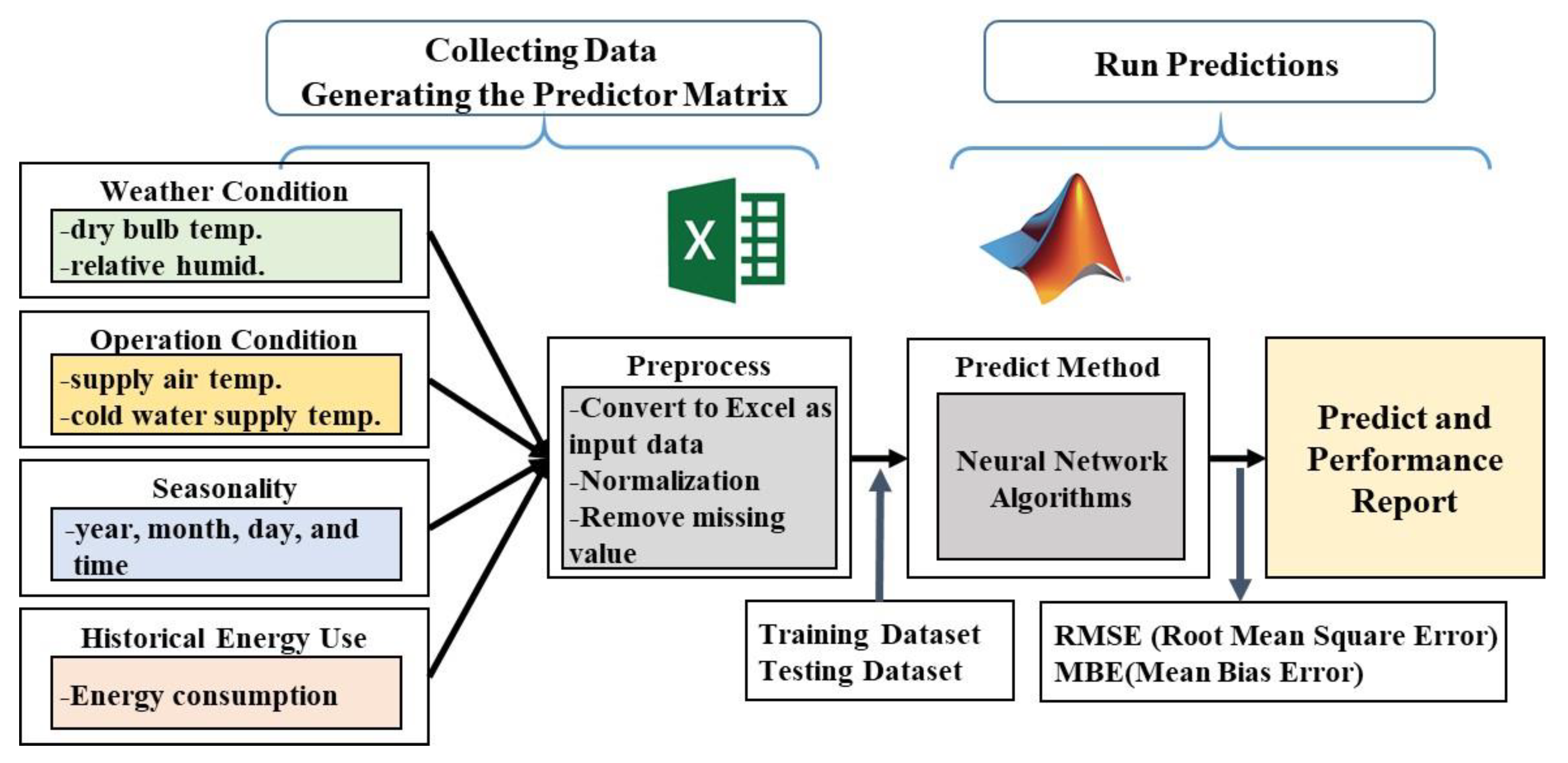
Figure 1 shows the process of predicting the energy consumption of the absorption heat pump. Data necessary for prediction is collected from the target building and changed to an appropriate form for use as input data. In this process, all data is preprocessed. In this way, input data are prepared to predict energy consumption using natural network algorithms. Finally, the predictive performance of each algorithm is evaluated through the prediction results.
2.1. Collection of Absorption Heat Pump Operational Data
The dataset used for training the neural network training algorithms is composed of absorption heat pump data that were measured during the heating period in an actual office building which is located in Seoul, Korea. The building is an office facility with a total floor area of 41,005.32 m2 and a total of 18 floors. An absorption heat pump with a capacity of 600 USRT is the heat source facility. From 10 December 2020 to 12 January 2021, weather data and absorption heat pump operation data were collected to predict the energy consumption of one absorbent heat pump operated during the heating period. All data were collected on an hourly basis, and for energy consumption, cumulative usage was used for an hour. The entire dataset was preprocessed before the prediction was performed. First, the entire dataset was normalized to a value in the range of 0 to 1, and missing values in which the air conditioning facility was not operated were removed. Energy consumption prediction was performed using 251 data points that were preprocessed in this way.
2.2. Neural Network Algorithms
The deep learning neural network training algorithms included in the Neural Networks Toolbox of MATLAB (R2021a) were adopted to predict energy consumption, and multilayer shallow neural network training algorithms were used as training algorithms. Multilayer neural network training data exhibit excellent performance when optimized using the gradient of the neural network’s performance with regard to neural network weights and the Jacobian matrix of the neural network error. The gradient and Jacobian matrix are calculated using a backpropagation algorithm. The backpropagation algorithm performs calculations by going backward through the neural network. The following twelve neural network training algorithms were compared to predict energy consumption: Levenberg–Marquardt (LM), Bayesian regularization (BR), Broyden–Fletcher–Goldfarb–Shanno (BFGS) quasi-Newton (BFG), resilient propagation (RP), scaled conjugate gradient (SCG), conjugate gradient backpropagation with Powell–Beale restarts (CGB), conjugate gradient backpropagation with Fletcher-Reeves updates (CGF), conjugate gradient backpropagation with Polak-Ribiére updates (CGP), one-step secant (OSS), gradient descent with momentum and adaptive learning rate (GDX), gradient descent with momentum (GDM), and gradient descent (GD) models.
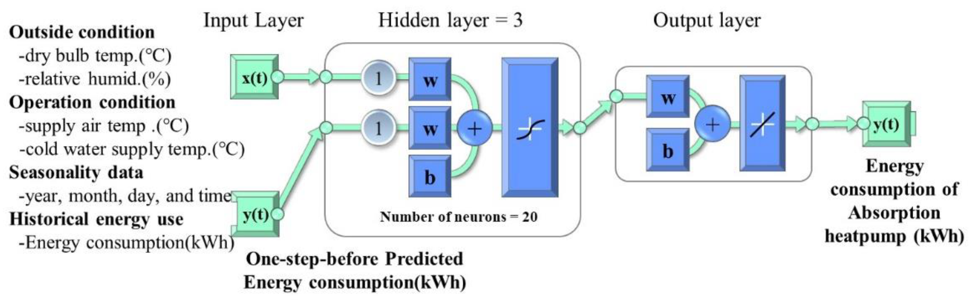
Figure 2 is a schematic diagram of the neural network used in this study, which is a two-layer feedforward neural network with a sigmoid transfer function in the hidden layer and a linear transfer function in the output layer. Neural network training algorithms are typically composed of an input layer, hidden layer, and output layer. This neural network also stores previous values of x(t) and y(t) sequences using tapped delay lines. Since y(t) is a function of y(t−1), y(t−2), …, y(t−d), the output y(t) of the neural network is fed back to the neural network input through delay.
For neural network learning in the input layer, outside conditions, seasonality data, historical energy consumption data, and energy consumption prediction results fed back from output layers are used as the input values. The hidden layer receives input signals every hour from the input layer and performs neural network calculations through internal neurons. The hidden layers were set to 3 and the number of neurons to 20. The output layer outputs the energy consumption (kWh) prediction result for an hour after the input signal point based on the hidden layer calculation result.
2.3. Prediction Criteria for Neural Network Training Algorithms
The input values are the dry bulb temperature of the outside air, relative humidity, cold water supply temperature, and water supply flow rate. The year and date were used as seasonality data.
The structural parameter is the state of the hidden layer and neuron in which actual learning takes place, and the learning capacity is determined according to the number. Epoch, a learning parameter that is used as a unit of learning, is defined as one complete pass through the entire data set.
Table 1 lists the conditions.
In order to obtain more accurate prediction results, missing values were removed due to the non-operation hours, and the dataset was normalized. A total of 250 data points from 10 December 2020 to 12 January 2021 were used for the analysis. All training data were normalized to values between 0 and 1.
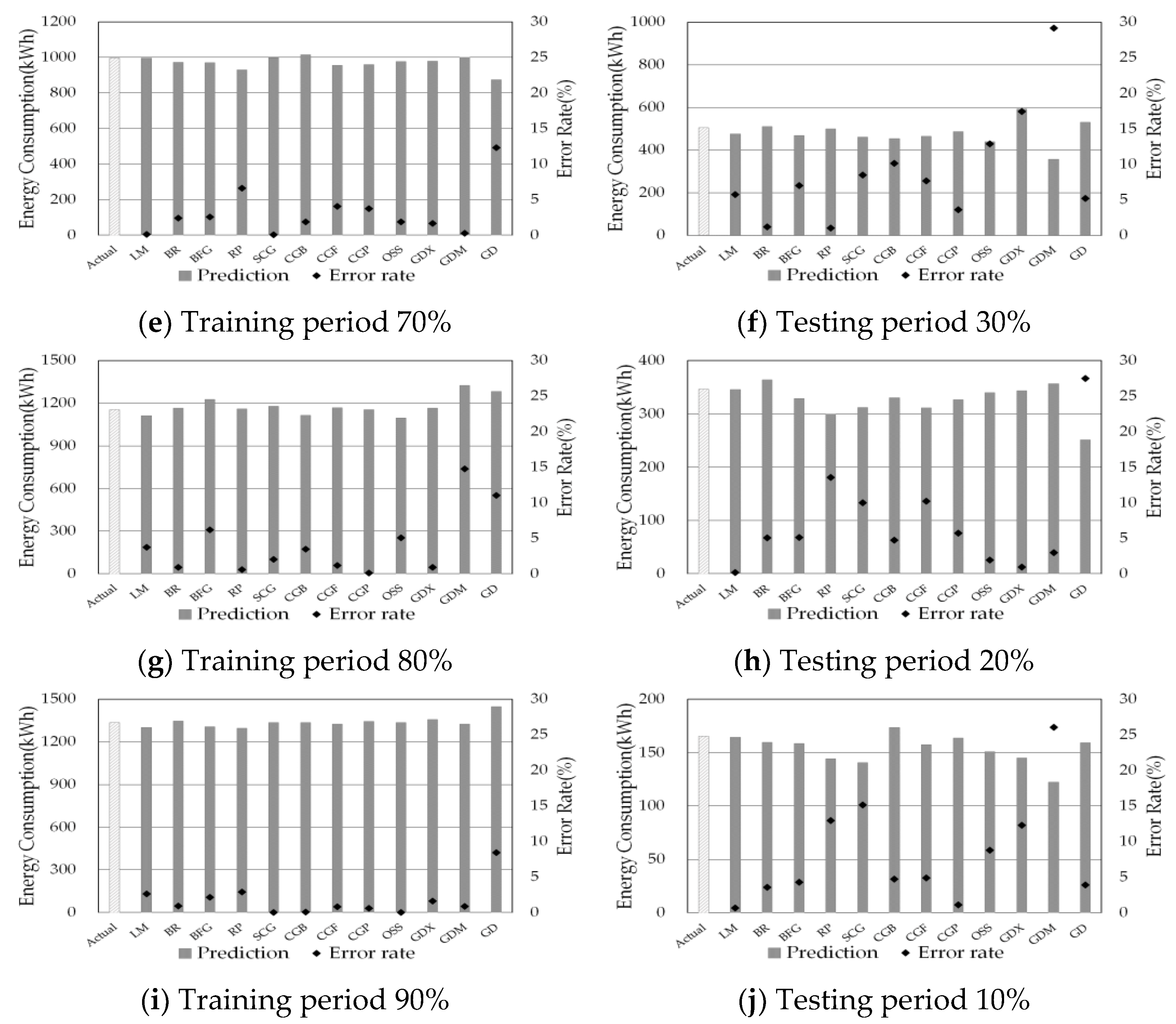
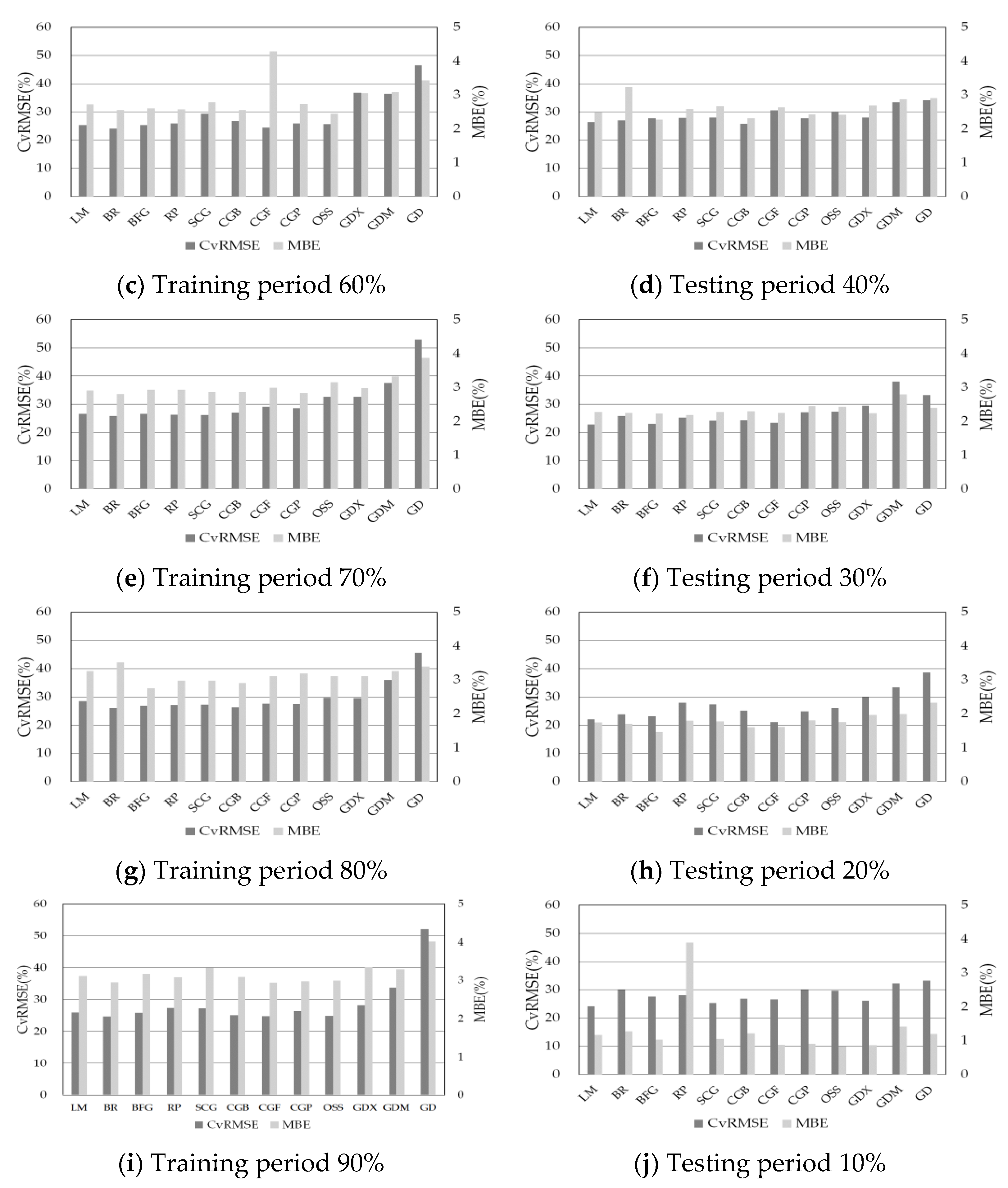
The training data size was changed from 50% to 90%, and thus, energy consumption could be predicted.
2.4. Performance Evaluation Indicators
The predictive performance of each model was evaluated according to ASHRAE Measurement and Verification (M&V) guidelines, the U.S. Department of Energy Federal Energy Management Program (FEMP) guidelines, and the International Performance Measurement and Verification Protocol (IPMVP).
Table 2 shows that ASHRAE, FEMP, and IPMVP present an M&V protocol for building energy management and serve to establish the Building Energy Model’s predictive accuracy criteria for predicting building energy performance. In this study, the CvRMSE and MBE were employed as performance indicators. CvRMSE refers to the degree of variance of the estimates, and MBE is an error analysis indicator that tracks how close estimates form a cluster to the target. Equations (1) and (2) present the formulas for obtaining the CvRMSE and MBE.
where
n is the number of data points,
p is the number of parameters,
is the utility data used for calibration,
is the simulation predicted data, and
is the arithmetic mean of the sample of
n observations.
4. Discussion
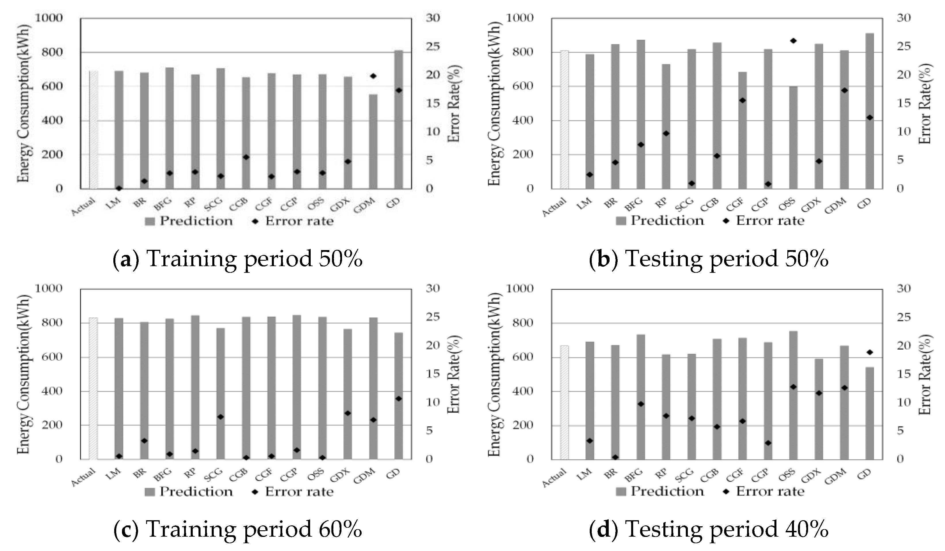
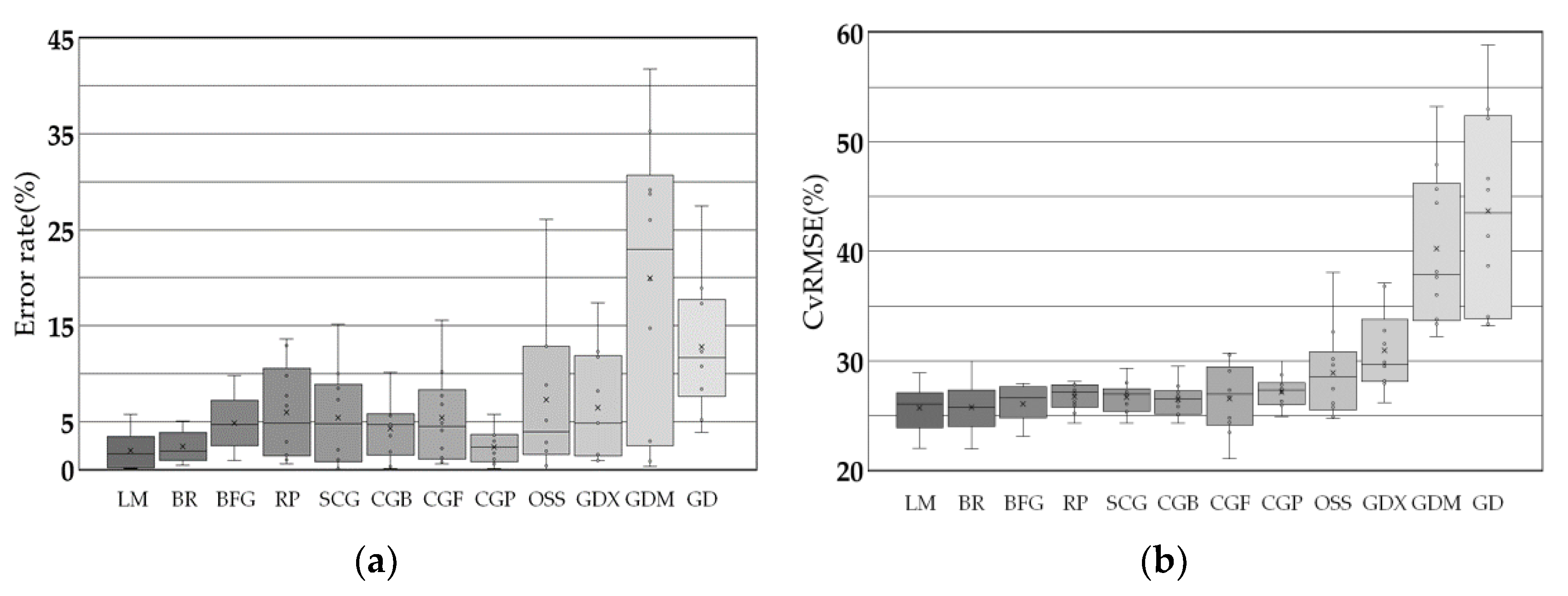
To determine how each algorithm changes its prediction performance with the change in training test data size,
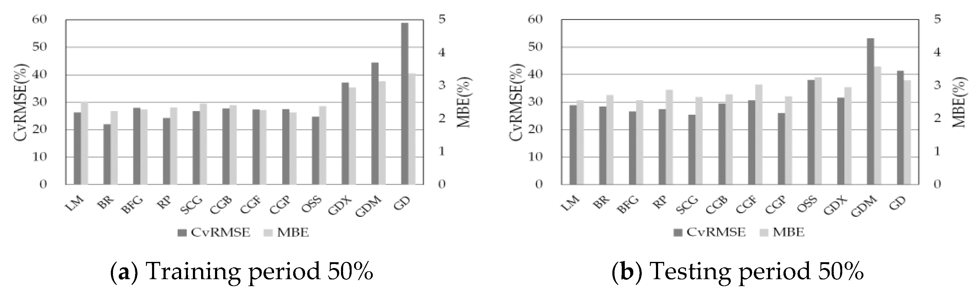
Figure 5a,b show the distribution of the error rate and CvRMSE, respectively, for the energy consumption prediction results under all conditions for each algorithm.
Table 3 provides a summary of the minimum, maximum, and standard deviations (SDs) of the error rate and CvRMSE for each algorithm. Based on the overall energy consumption predictions, LM, BR, and CGP showed the best results in terms of the distribution of the error rates. LM showed an SD of 1.94 with a minimum error rate of 0.09% and a maximum error rate of 5.76 percent. BR showed a minimum error rate of 0.41% and a maximum of 5.05%, with an SD of 1.68, and CGP showed a minimum error rate of 0.13% and a maximum of 5.73%, with an SD of 1.76. The other algorithms showed high error rates of 9.78~41.77%, among which OSS had the worst results with 8.16 SD, followed by GDM with 41.77 SD and GD with 27.52 SD.
For CGF, OSS, GDX, GDM, and GD, the CvRMSE SDs of the prediction results are 3.13~9.08, confirming that the prediction performance of these algorithms was poor. The other algorithms had SDs of 1.27~2.33 and exhibited predictive performances that satisfy ASHRAE Guideline 14. When the error rate and CvRMSE results are combined, LM and BR exhibit the best prediction performance. These two models are known to be suitable for nonlinear regression problems [
25,
26], which is confirmed in this study as well.
Models such as GDX, GDM, and GD, which are gradient-based methods, are algorithms that find the minimum value of a function through the gradient of the loss function. One of the disadvantages of this gradient descent method is the local minima problem. This problem occurs when it is difficult to find a unique minimum value because the graph of the loss function becomes complex, which is known to be mainly due to the learning rate. Among the gradient-based algorithms, the significantly poor prediction performance of GDM and GD is considered to have caused this problem.
As such, in this study, the multilayer neural network algorithms of the same series show different prediction performance even under the same conditions. Therefore, when applying a multilayer neural network algorithm to a project, an appropriate algorithm that can obtain the best results must be selected by considering the type and amount of data to be predicted.
5. Conclusions
In this study, the ability of twelve multilayer neural network algorithms under the same conditions were compared and evaluated to predict the energy consumption of an absorption heat pump in an air conditioning system. A predictive model using twelve shallow multilayer neural network algorithms was developed. The monthly heating operation data of the absorbent heat pump were compared and evaluated with the prediction performance of each algorithm according to data training size.
The energy consumption was compared and evaluated with the prediction performance of various shallow multilayer neural network training algorithms based on backpropagation algorithms using measured data and confirmed that the prediction performance differs for each model. LM and BR, which are generally known to be suitable for nonlinear regression predictions, exhibited the best predictive performance among the models studied because they satisfy ASHRAE Guideline 14 and also had low error percentages in the results. On the other hand, the error in the prediction results for GDM and GD, the gradient-based methods, was large, and their prediction performance was poor enough not to satisfy ASHRAE Guideline 14 under all conditions.
Based on these results, the prediction performance may differ for each model, even for multilayer neural network training algorithms that are based on the same backpropagation algorithms. Applying the prediction algorithm to the field may change the amount of collected data and the prediction period, so stable results must be obtained even if the ratio of training and testing period changes. In the field of HVAC facilities, energy consumption, heating and cooling loads, etc., which are major predictions, are in the form of time series, so it would be advantageous to apply nonlinear regression prediction models such as Levenberg–Marquard backpropagation (LM) and Bayesian regulation backpropagation (BR). In addition, despite the use of a small amount of data of (251 data points) for training, it was confirmed that predictive performance that satisfies the criteria of ASHRAE guideline 14 could be obtained by selecting an appropriate algorithm. Therefore, in order to carry out the project and obtain the best results, an appropriate model must be selected in consideration of the characteristics of the project.
Machine learning algorithms work well for data used to train models, but overfitting may occur that is not properly generalized in new data. In this study, the amount of data was limited, so it was not possible to test whether the model was overfit. In future studies, more dates will be secured to conduct research on the development of better performance prediction models.


