A Nonintrusive Load Monitoring Method for Office Buildings Based on Random Forest

Abstract

Load monitoring can help users learn end-use energy consumption so that specific energy-saving actions can be taken to reduce the energy consumption of buildings. Nonintrusive monitoring (NIM) is preferred because of its low cost and nondisturbance of occupied space. In this study, a NIM method based on random forest was proposed to determine the energy consumption of building subsystems from the building-level energy consumption: the heating, ventilation and air conditioning system; lighting system; plug-in system; and elevator system. Three feature selection methods were used and compared to achieve accurate NIM based on weather parameters, wavelet analysis, and principal component analysis. The implementation of the proposed method in an office building showed that it can obtain the subloads accurately, with root-mean-square errors of less than 46.4 kW and mean relative errors of less than 12.7%. The method based on weather parameters can provide the most accurate results. The proposed method can help improve the energy efficiency of building service systems during the operation or renovation stage.

1. Introduction

Buildings can account for 50% of the total energy consumption of society and 30% of greenhouse gas emissions [1]. Therefore, decreasing the energy consumption of buildings plays a key role in sustainable development. For buildings, the energy consumption mainly includes embodied energy and operational energy. The embodied energy consists of energy used in the process of manufacturing building material, constructing buildings, and destructing buildings [2]. The operational energy often results from the heating, ventilation, and air conditioning (HVAC) system; lighting system; plug-in system; and elevator system [3], which accounts for 80–90% of the life-cycle energy consumption [4]. By reducing the operational energy, life-cycle energy can decline obviously. For existing buildings in operation, performance evaluation and renovation projects play an important role in reducing operational energy consumption and carbon emission.

Monitoring the energy consumption of subsystems is an effective approach to evaluate building efficiency and provide guidance for renovation. A study showed that detailed feedback information from monitoring systems could be provided for users, which can encourage energy-saving behavior, improve energy management, and upgrade fault diagnosis [5]. Buildings can achieve more than 10% of potential carbon savings by obtaining details on energy consumption, indicating its importance in energy management [6].

The general approach to obtain device-level energy consumption is to install sensors for the devices of interest, which is called intrusive monitoring [5]. Although the approach can obtain accurate data on energy consumption, it is expensive and complex with privacy concerns [7,8,9]. A more promising approach for monitoring the individual energy consumption of devices is nonintrusive monitoring (NIM). NIM measures only the total power consumption and the energy consumption of each appliance, which is calculated by intelligent algorithms [10,11]. After it was first proposed by Hart [12], many algorithms have been introduced into NIM approaches, such as hidden Markov models [10], discriminative sparse coding [13], deep learning [14], random forest (RF) [15], and neural networks [16]. A NIM method based on a decision bagging tree classifier was proposed in [17], which applies principal component analysis (PCA) to extract the fused time-domain features. The proposed method showed excellent performance on three real household datasets with an accuracy of over 98%. A convolutional neural network-based NIM model with differential input was applied to appliance-level load monitoring in residential buildings [18]. The model accurately identified the energy consumption of refrigerators, microwaves, and dishwashers with a low mean square error (MSE) and mean absolute error. A NIM algorithm based on Karhunen-Loeve expansion was proposed to disaggregate household appliances using voltage-specific appliance signatures to ensure the accuracy of disaggregation in the case of large voltage fluctuations [19]. The disaggregation algorithm yielded accurate results with an average accuracy of over 92.5%, even under severe voltage fluctuations. A hybrid NIM algorithm was proposed for residential power load disaggregation, which combined factorial hidden Markov models and iterative subsequence dynamic time warping to accurately identify the characteristics of appliances and decrease the intrusiveness of offline training [20]. The approach can accurately disaggregate multiple operating appliances and performed better than the existing factorial hidden Markov model benchmark. Current research has focused on residential buildings rather than commercial buildings because most domestic appliances have limited states (on/off or multiple stages), where their loads are easy to obtain from the total load. However, commercial buildings consume large quantities of energy and it is necessary to monitor their energy consumption for energy conservation.

In office buildings, there are four main subsystems, namely HVAC systems, lighting systems, elevator systems, and plug-in systems. The HVAC system provides a comfortable indoor environment for occupants, and its load results from outdoor parameters and occupant activities. The lighting system provides occupants with a comfortable luminous environment. Its load is associated with the usage duration and type of lighting devices. The elevator system performs the function of transportation in office buildings and its load is mainly influenced by the commute time. The plug-in system includes plug-in office devices such as desktops, printers, and copiers. Its load is determined by the usage duration and rated power consumption of these devices. The energy consumption data of these subsystems would provide useful information on the energy efficiency and usage of buildings, such as typical and atypical operating conditions and characterizing dynamics in building operations. The information obtained can help energy managers develop dynamic solutions for the optimal control of subsystems and targeted energy efficiency measures to improve the performance of subsystems. Results have shown that this optimal control can help save 10% of energy for HVAC systems [21] and up to 50% of energy for lighting systems [22].

Research on NIM in commercial buildings began in 1996 [23]. The energy consumption of commercial buildings can be divided into the energy consumption of different subsystems according to the services provided by the buildings, including loads of the HVAC system, elevator system, plug-in system, and lighting system. A NIM method was proposed to obtain the energy consumption of a lighting system based on virtual submetering disaggregation [24]. The results showed that the data analytics method can accurately monitor the energy consumption of the lighting system, and the relative difference between the disaggregation results and monitoring data was less than 5%. A NIM method based on an event detection algorithm was developed, which identified the state and type of appliances and then calculated the required electric power of lighting systems [25]. A NIM framework was developed to identify the energy consumption of HVAC systems [26]. The energy consumption of plug-in devices and lighting systems was first modeled by the Fourier series, and then the energy consumption of the HVAC system was calculated by subtracting it from the total energy consumption. A NIM model was proposed to obtain the plug-in load in an office building [27]. The model could identify the profiles of the measured appliances and found those with significant impact in buildings. Most research has focused on one type of energy-use system, while few have reported the disaggregation of building-level energy consumption into more detailed subloads. Detailed information is important to coordinate the operation of the four subsystems and improve the efficiency of buildings.

The above review shows that NIM can be applied to obtain subsystem load information for operation optimization. However, system-level NIM needs further exploration due to the following gaps:

• Most research has mainly concentrated on how to identify the states, types, and energy use of devices in residential buildings. There are limited studies on system-level disaggregation in office buildings, which can provide detailed information on system operation optimization.
• Existing NIM research on commercial buildings has focused on one type of subsystem, while studies on multiple subsystem load disaggregation from building-level energy data are limited. Thus, it is necessary to propose a new NIM method to determine the energy consumption of multiple subsystems (i.e., the four main subsystems).

In this study, a NIM method based on RF was proposed to obtain the energy consumption details of multiple subsystems in office buildings from the total energy consumption data. RF belongs to an ensemble approach and produces the final result by averaging the output of a series of independent weak learners. RF was used in the study because of its stable nonlinear mapping ability with easy parameter tuning [28]. The total energy consumption of an office building was disaggregated into four parts based on their function and operation characteristics: the HVAC system, lighting system, plug-in system, and elevator system. Based on the information provided by this method, the performance of each subsystem can be determined, and the corresponding energy efficiency measures can be taken to improve their performance. Feature selection influences the accuracy of NIM models, so three feature selection methods were used and compared in this study to improve the accuracy of the NIM model.

The remainder of this paper is organized as follows. Section 2 presents the NIM method and the steps based on RF. In Section 3, an office building is used as a case study to verify the proposed method. Section 4 presents the disaggregation results based on different feature selections. The conclusions is displayed in Section 5.

2. The NIM Approach Based on Random Forest

In this study, RF was applied to perform the NIM. RF is an ensemble learning algorithm that consists of several tree-based weak learners that are built independently to simultaneously decrease variances and biases [29]. It adopts bootstrap resampling to generate several training sets. Each tree is developed based on these training sets with random feature selection at every split, which ensures diverse results for each tree [30]. The final output is the average of the results for all the trees, as shown in Equation (1). RF is widely applied in classification and regression problems, such as energy forecasting and load identification [31,32]. The framework of the NIM method based on RF is shown in Figure 1 and the primary steps are introduced in detail.

$$\mathrm{y}=\frac{{\displaystyle {\sum }_1^C{T}_i(x)}}{C}$$

(1)

where x are the inputs of every tree, C is the number of developed trees, T_i(x) are the outputs of every tree, and y are the results of RF.

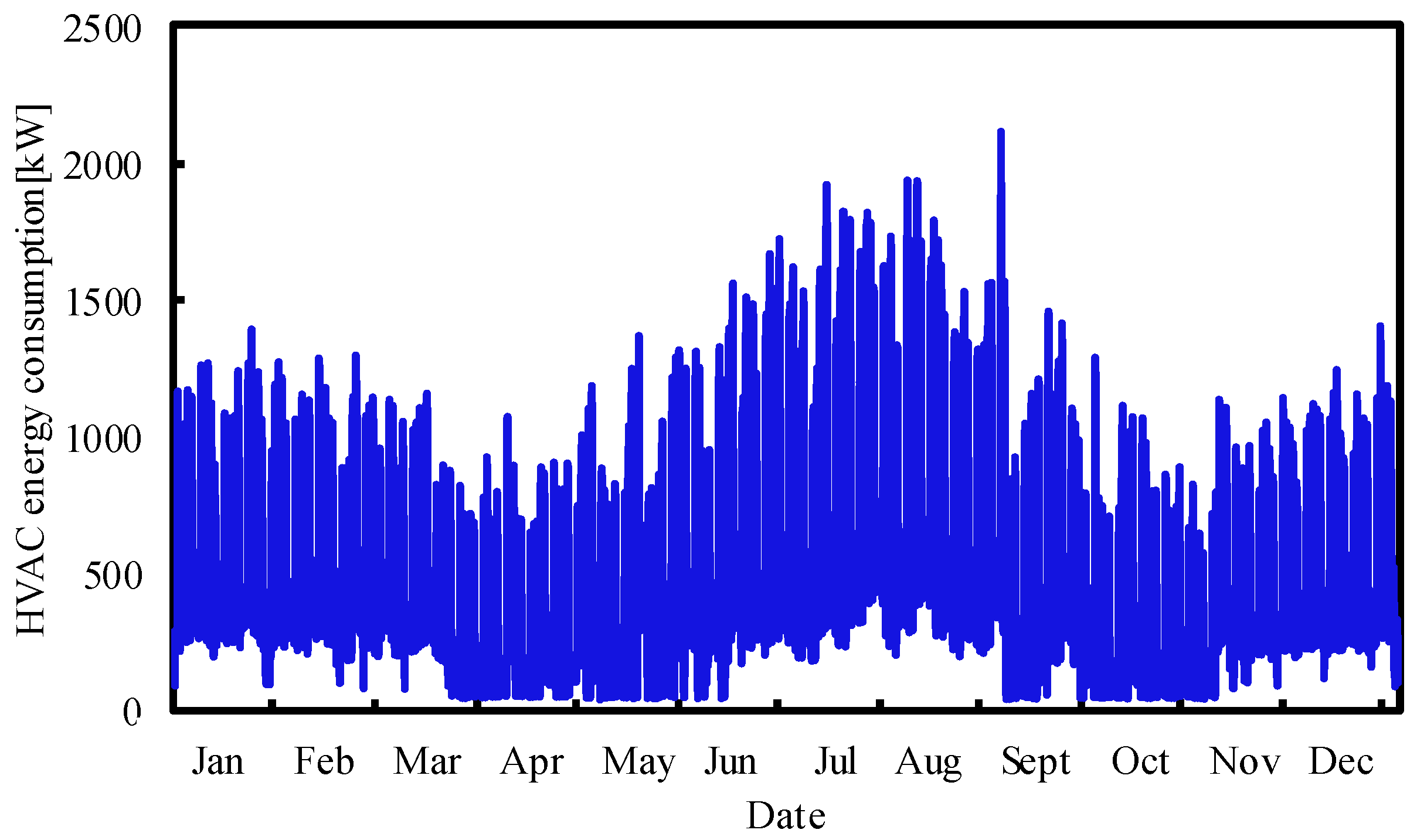
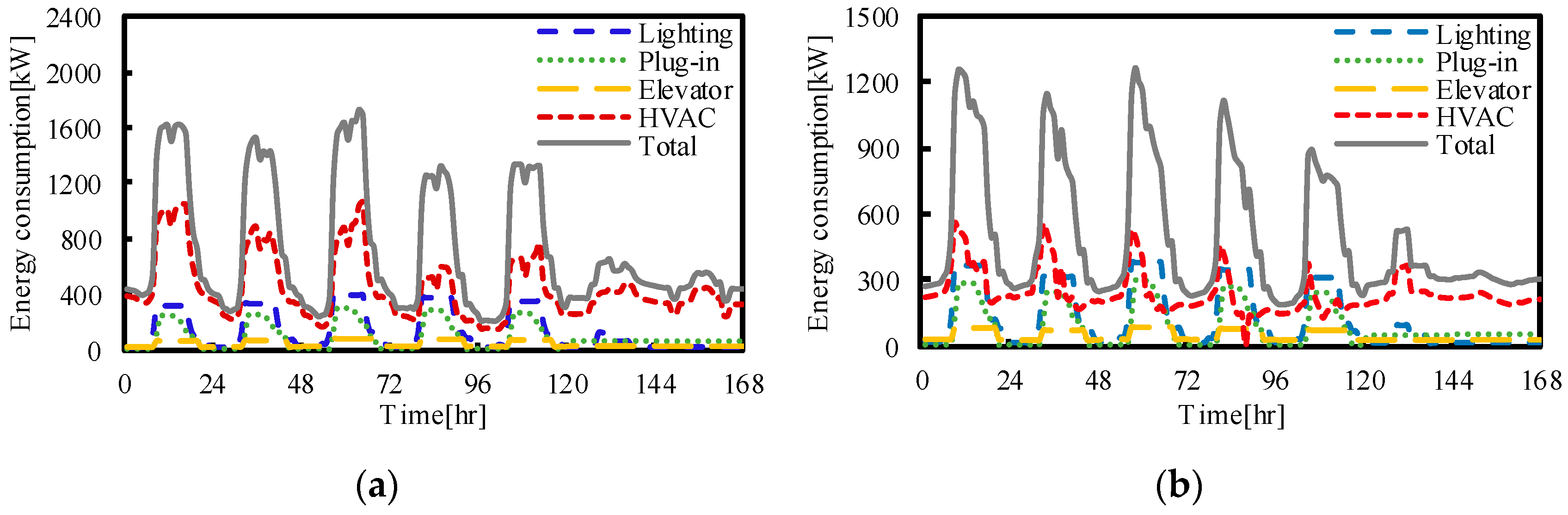
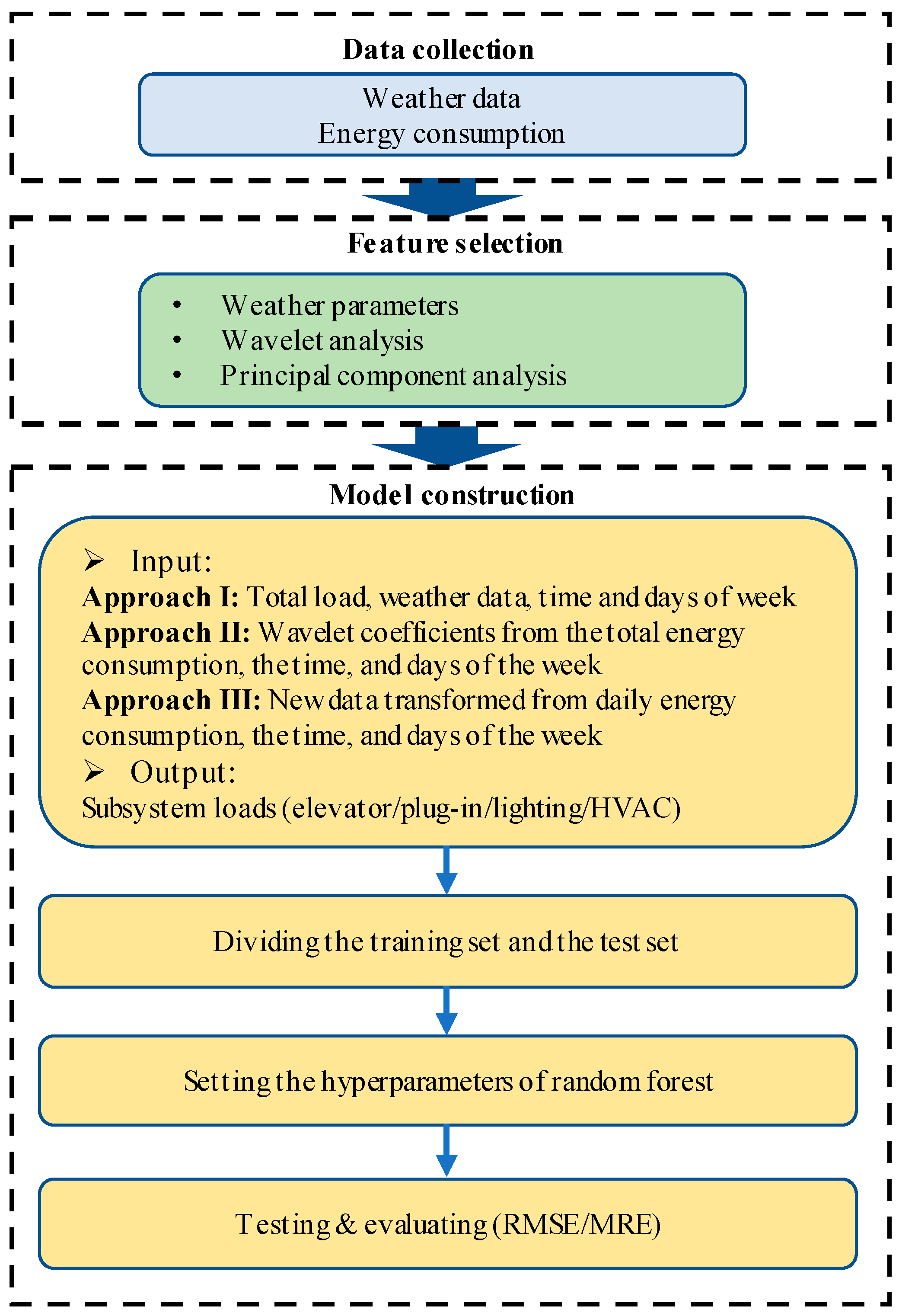
2.1. Data Collection

The first step is to collect the data including the weather data and energy consumption. Weather data include dry-bulb temperature and relative humidity because they are related to the cooling/heating demand of buildings and influence the energy consumption of HVAC systems. Energy consumption includes the total energy consumption and the energy consumption of subsystems. The total energy consumption can be used to extract features to disaggregate subsystem load while the energy consumption of subsystems is applied to train and test the approach.

2.2. Feature Selection

The total energy consumption was disaggregated into four types of subsystem loads (i.e., loads of the HVAC system, elevator system, plug-in system, and lighting system). Time is an influential factor and was included in the inputs because it is closely related to the utilization of these subsystems. These subsystems are frequently used during, instead of after, working hours. For the HVAC system load, weather conditions significantly influence the heat gain and loss into the indoor environment. Hence, weather data should be considered as another input. However, weather data may not be monitored in practice, in which case wavelet analysis and PCA are applied to extract features from the total energy consumption. Therefore, three types of inputs are discussed in this study.

(1) Approach I

If weather data are monitored, the total energy consumption, dry-bulb temperature, relative humidity, and the time and days of the week are taken as inputs. This approach considers factors that are directly related.

(2) Approach II

Wavelet analysis is used to extract information hidden in the total energy consumption. Wavelet analysis is a common tool to disaggregate the original series and improve model accuracy in load forecasting [33]. A series of functions are used to represent data or functions [34]. The theory behind this is to obtain information at different scales or resolutions by high-pass and low-pass filters and to produce a series of wavelet coefficients that contribute to extracting characteristics in the frequency domain. In this approach, the total energy consumption is disaggregated into low-frequency coefficients (approximation) and high-frequency coefficients (details) using wavelet analysis at level 1, as shown in Equation (2) [35]. Then, the wavelet coefficients from the total energy consumption, time, and days of the week are taken as inputs.

$$y(t)={\displaystyle \sum _k{{\displaystyle s}}_{j_n,k}{{\displaystyle \phi }}_{j_n,k}(t)+}{\displaystyle \sum _{j>j_n}{\displaystyle \sum _k{{\displaystyle d}}_{j,k}{{\displaystyle \varphi }}_{j,k}(t)}}$$

(2)

where ${\phi }_{j_n,k}\left(t\right)$ and ${\varphi }_{j,k}\left(t\right)$ represent the bases of scaling functions and wavelets, and $S_{j_n,k}$ and $d_{j,k}$ represent low-frequency and high-frequency coefficients.

(3) Approach III

PCA is used as the feature extraction method. PCA is a general approach to handle multivariate problems in raw data for load prediction and NIM [36]. PCA transforms the observed values into nonlinearly correlated principal components, which are sorted in descending order according to their variability [37]. The theory of PCA can be expressed in Equation (3). In this approach, the daily total energy consumption is considered as 24 features that are then projected to a lower-dimensional space spanned by four principal components obtained from PCA. The rationale behind the four principal components is that these can represent the four types of subsystem loads without increasing the computational complexity. The new data transformed from daily energy consumption, time, and days of the week are considered as Approach III.

$$\begin{array}{cc}\hfill X& =S{L}^{\prime }+R\hfill \\ & ={\displaystyle \sum _1^Q{s}_i{l}_i^{\prime }}+R\hfill \end{array}$$

(3)

where X represents an (M N) matrix, s_i is the ith principal component’s score vector, l_i is the ith principal component’s loading vector, and R represents an (M N) residual matrix. S is an (M Q) matrix of M scores on Q principal components, and L is an (N Q) matrix of N loadings on Q principal components.

2.3. Model Construction

The NIM method based on RF was modeled in the scikit-learn [38] module in Python. The adjustable hyperparameters included the number of estimators, the maximum depth of individual trees, the number of features, the minimum samples for a split, and the minimum sample leaf. The RF models are relatively sensitive to the number of estimators and the maximum depth of individual trees, so they were adjusted for improved model performance [39]. The remaining hyperparameters were set to the default values. The number of estimators is relevant to the number of weak learners and the computation requirements. The maximum depth of individual trees depends on the data characteristics and deeper trees can have better performance [40]. A grid search was applied to identify the optimal hyperparameters [41]. More detailed hyperparameters are listed in Section 3.

To evaluate the NIM results, two evaluation indices (MRE and RMSE) were used, as shown in Equations (4) and (5). The MRE measures the relative bias of the models, while the RMSE quantifies the absolute deviation.

$$RMSE=\sqrt{\frac{1}{N}{\displaystyle \sum }_{i=1}^N{(\widehat{y_i}-y_i)}^2}$$

(4)

$$MRE=\frac{{{\displaystyle \sum }}_{i=1}^N\left|\widehat{y_i}-y_i\right|}{{{\displaystyle \sum }}_{i=1}^N\left|y_i\right|}$$

(5)

where $\widehat{y_i}$ is the disaggregation load of the NIM model, $y_i$ is the actual value, and N is the number of samples.

2.4. Implementation of the Method

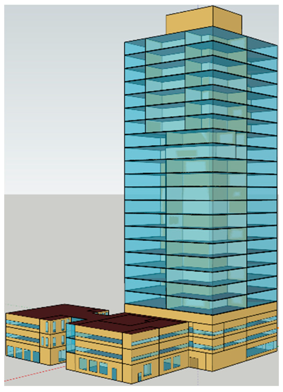
When all necessary data are collected, the whole implementation of the method works as the following process:

Step 1: The obtained data are preprocessed to extract the features used for model input. For Approach I, the total energy consumption, dry-bulb temperature, relative humidity, and the time and days of the week are integrated as the inputs. For Approach II, the total energy consumption is disaggregated into low-frequency coefficients and high-frequency coefficients using wavelet analysis at level 1 first. The wavelet coefficients from the total energy consumption, time, and days of the week are taken as inputs. For Approach III, the daily total energy consumption is projected to a lower-dimensional space spanned by four principal components obtained from PCA. The new data transformed from daily energy consumption, time, and days of the week are considered as inputs.

Step 2: The extracted features are integrated with the corresponding subsystem load to form the sample set. Then, 80% of samples are used as the training set and the remainder are used as the testing set.

Step 3: The RF model is trained based on the training set and the hyperparameters are adjusted using grid search.

Step 4: The model is tested based on the testing set and RMSE, and MRE is used to evaluate the accuracy of the model.

3. Case Study

An office building located in a hot summer and cold winter region was chosen to demonstrate the performance of the load disaggregation approach. The building covered an area of approximately 32,000 m², with 23 floors above the ground, and the physical model of the building was modeled in Google Sketchup, as shown in Figure 2. The window-wall ratio of the whole building was approximately 74% and the story height was 4 m.

In the office building, there are four main subsystems, namely the HVAC system, the lighting system, the elevator system, and the plug-in system, and related parameter settings, including building physical information and internal heat gain, are shown in

Table 1. The related parameter settings in the building.

Building Envelope
Item	Model Thermal Property (W/m2 K)		Reference
Interior floor	1.5		[42]
Interior wall	0.16
Interior ceiling	1.5
Exterior door	1.2
Exterior floor	0.23
Exterior window	2.3
Exterior wall	0.45
Internal heat gain
Item	Design density	Schedule	Reference
Occupant	Office: 8 m2/person Hall: 20 m2/person	Weekdays: 1:00–600: 0% 7:00: 10% 8:00: 20% 9:00–12:00: 95% 13:00: 50% 14:00–17:00: 95% 18:00: 30% 19:00–22:00: 10% 23:00–00:00: 5% Weekends: 1:00–6:00: 0% 7:00–18:00: 5% 19:00–00:00: 0%	[42,43,44]
Lighting	Office: 18 W/m2 Hall: 11 W/m2	Weekdays: 0:00–5:00: 5% 6:00–7:00: 10% 8:00: 30% 9:00–17:00: 90% 18:00: 50% 19:00–20:00: 30% 21:00–22:00: 20% 23:00: 10% Weekends: 0:00–23:00: 5%
Plug-in devices	Office: 13 W/m2 Hall: 5 W/m2	Weekdays: 0:00–8:00: 2% 9:00: 40% 10:00–14:00: 90% 15:00: 80% 16:00: 70% 17:00–18:00: 50% 19:00–20:00: 30% 21:00–23:00: 2% Weekends: 0:00–23:00: 20%
Elevator	30 W/m2	Weekdays: 0:00–8:00: 32% 9:00–20:00: 100% 21:00–23:00: 32% Weekends: 0:00–23:00: 34%

. Considering the randomness of occupant behavior, ±20% of perturbations were added to the daily basic schedule.

The energy consumption of the HVAC system was estimated based on cooling/heating load and terminal equipment, while the energy consumption of the lighting system, the elevator system, and the plug-in system was calculated based on the design level and the schedule. For the calculation of the energy consumption of the HVAC system, the cooling and heating loads were simulated in EnergyPlus first. The energy consumption of the HVAC system consists of the energy consumption of chillers, chilled water pumps, and cooling water pumps. They are calculated based on Equations (6)–(11) [45].

$$E_{chiller}=\frac{Q_{cooling/heating}}{COP}$$

(6)

$$COP=a{x}^3+b{x}^2+cx+d$$

(7)

$$E_{chilled\_pump}=\rho gfh=gmh$$

(8)

$$m=\frac{Q_{cooling/heating}}{c\Delta t}$$

(9)

$$E_{cooling\_pump}=\frac{E_{chiller}+Q_{cooling/heating}}{E_{chiller}}$$

(10)

$$E_{HVAC}=E_{chiller}+E_{chilled\_pump}+E_{cooling\_pump}$$

(11)

where E_chiller, E_{chilled_pump}, E_{cooling_pump}, and E_HVAC are the energy consumption of the chillers, chilled water pumps, cooling water pumps, and HVAC systems, respectively; Q_{cooling/heating} is the cooling and heating loads of the office building; COP is the coefficient of performance of the chillers; x is the part load ratio of the chillers; a, b, c, and d are fitting coefficients between the COP and part load ratio of the chillers; g is the gravitational acceleration; m is the mass flow rate; h is the pump lift; c is the heat capacity of water; and ∆t is the temperature difference between supply and return water from the chillers.

The related parameters about the energy consumption of the HVAC system were chosen as follows: for Equation (7), a, b, c, and d were 3.9, −11.9, 12.1, and 1.1, which were obtained from a fitting of a chiller sample. For Equation (8), g was 9.8 m/s² and h was 60 m. For Equation (9), c was 4.2kJ/kg K and ∆t was 5 K.

The energy consumption of the elevator system, plug-in system, and lighting system was calculated by schedule, design density, and floor area, as shown in Equation (12).

$$E=cof\times density\times area$$

(12)

where E is the energy consumption of the elevator system, plug-in system, and lighting system; density is the design density of the elevator system, plug-in system, and lighting system; and area is the related area of design density.

The annual hourly energy consumption is shown in Figure 3. The load varies greatly during the entire year, i.e., higher in summer than in winter, with a peak of 2099.9 kW. Figure 4 shows the total loads and four subsystem loads in a typical week for winter and summer. The total load peaks at 9:00–18:00. The valley periods are 1:00–7:00 and 22:00–24:00 because of the working hours. The loads from the HVAC system vary significantly and are influenced by the weather and schedule. The profiles of the total load and HVAC system load are similar because the load fluctuations mainly result from the HVAC system. Loads of lighting, plug-in devices, and elevators regularly fluctuate owing to the periodic schedules of occupants.

The NIM models based on RF for the building were built in Python. A single RF model was built for every approach to obtain the individual energy consumption of each subsystem. A grid search was conducted to search for the optimal hyperparameters, where the number of estimators and the maximum depth of individual trees ranged from 10 to 200 and 1 to 30, respectively. All optimized hyperparameters applied in the study are listed in

Table 2. The RF-optimized hyperparameter setting for three approaches.

Hyperparameters	Setting
	Approach I	Approach II	Approach III
The number of estimators	152	143	181
The maximum depth of individual trees	13	18	21
The number of features	auto
The minimum samples for a split	2
The minimum sample leaf	1

. For reproducible results, the random state (the seed used by the random number generator) was fixed at a certain value.

4. Results and Analysis

The performance of the proposed NIM method is discussed in this section. The disaggregation results based on three feature selection approaches are first introduced, and the accuracy for each subsystem load is analyzed. Then, the performance of the models based on the three approaches is compared and discussed.

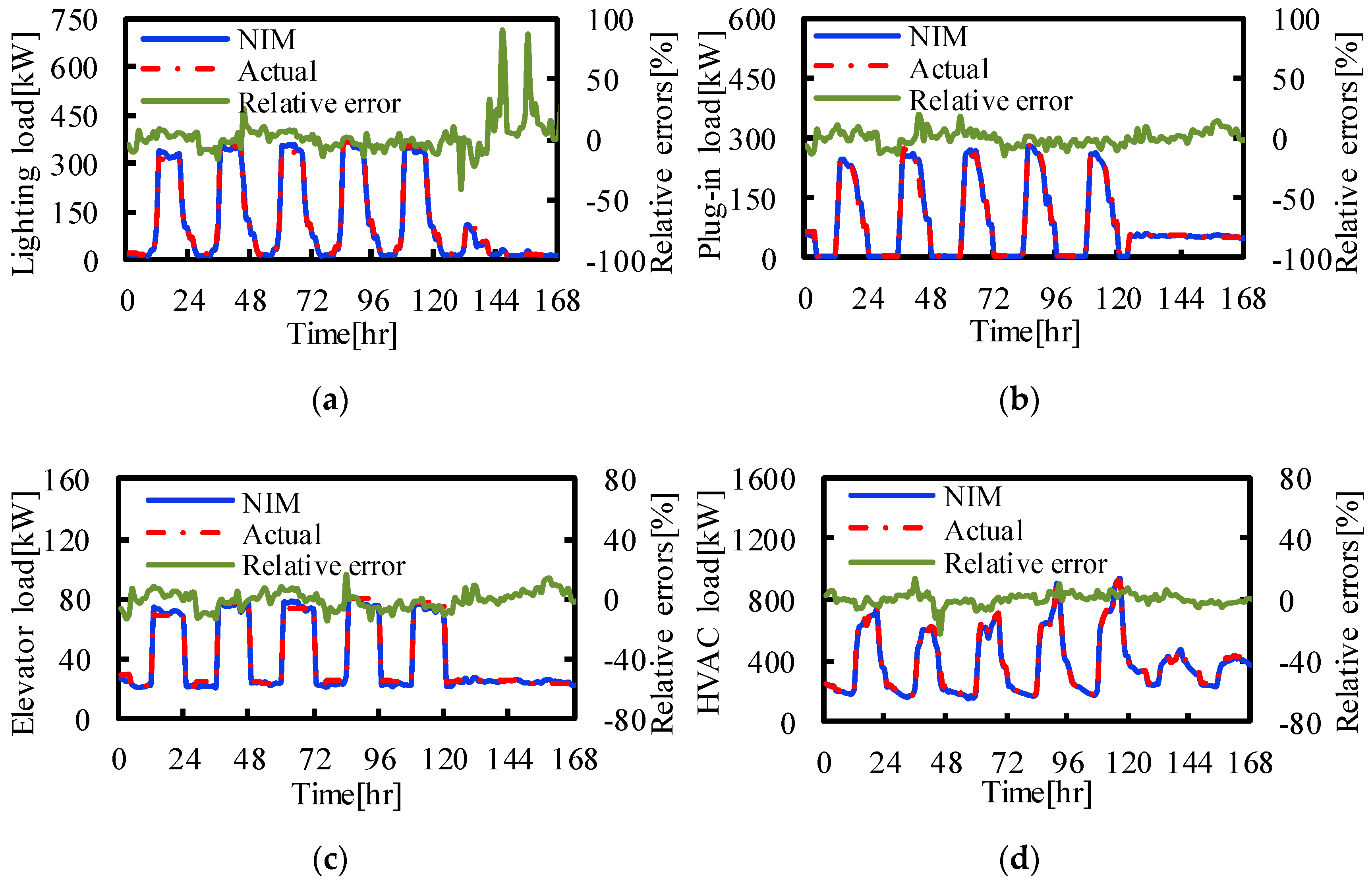
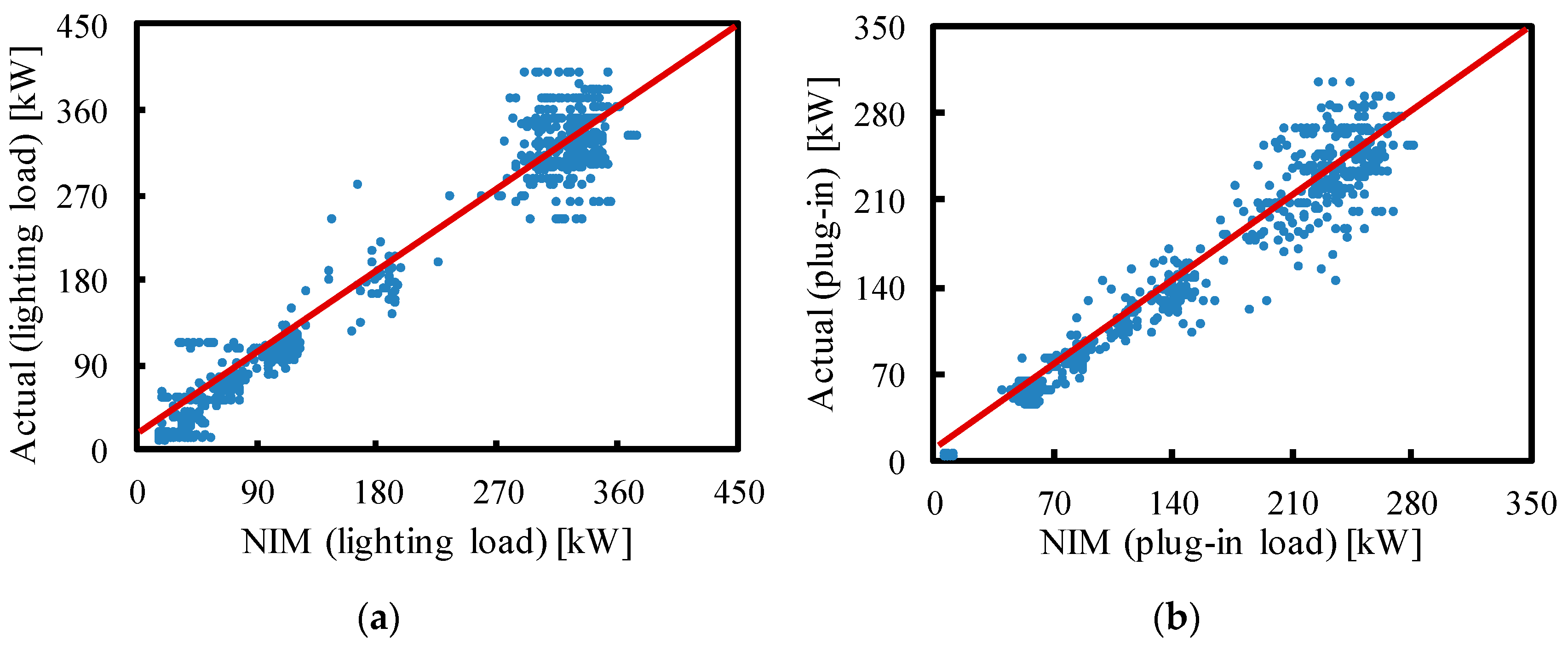
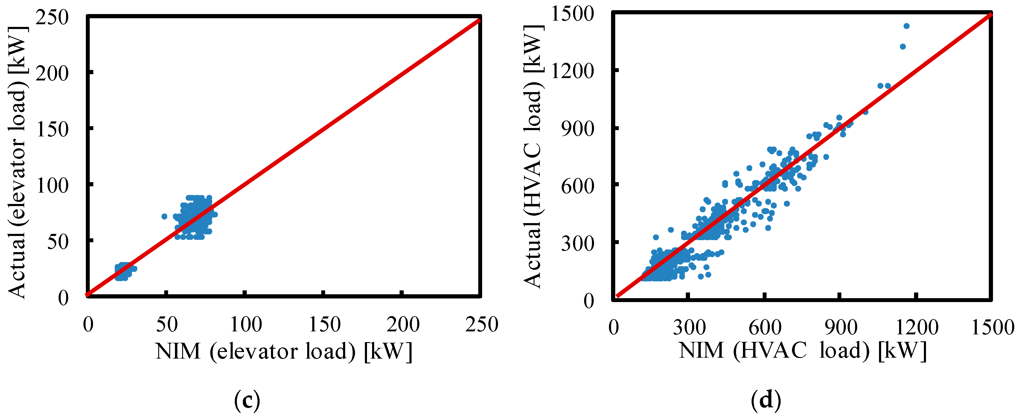
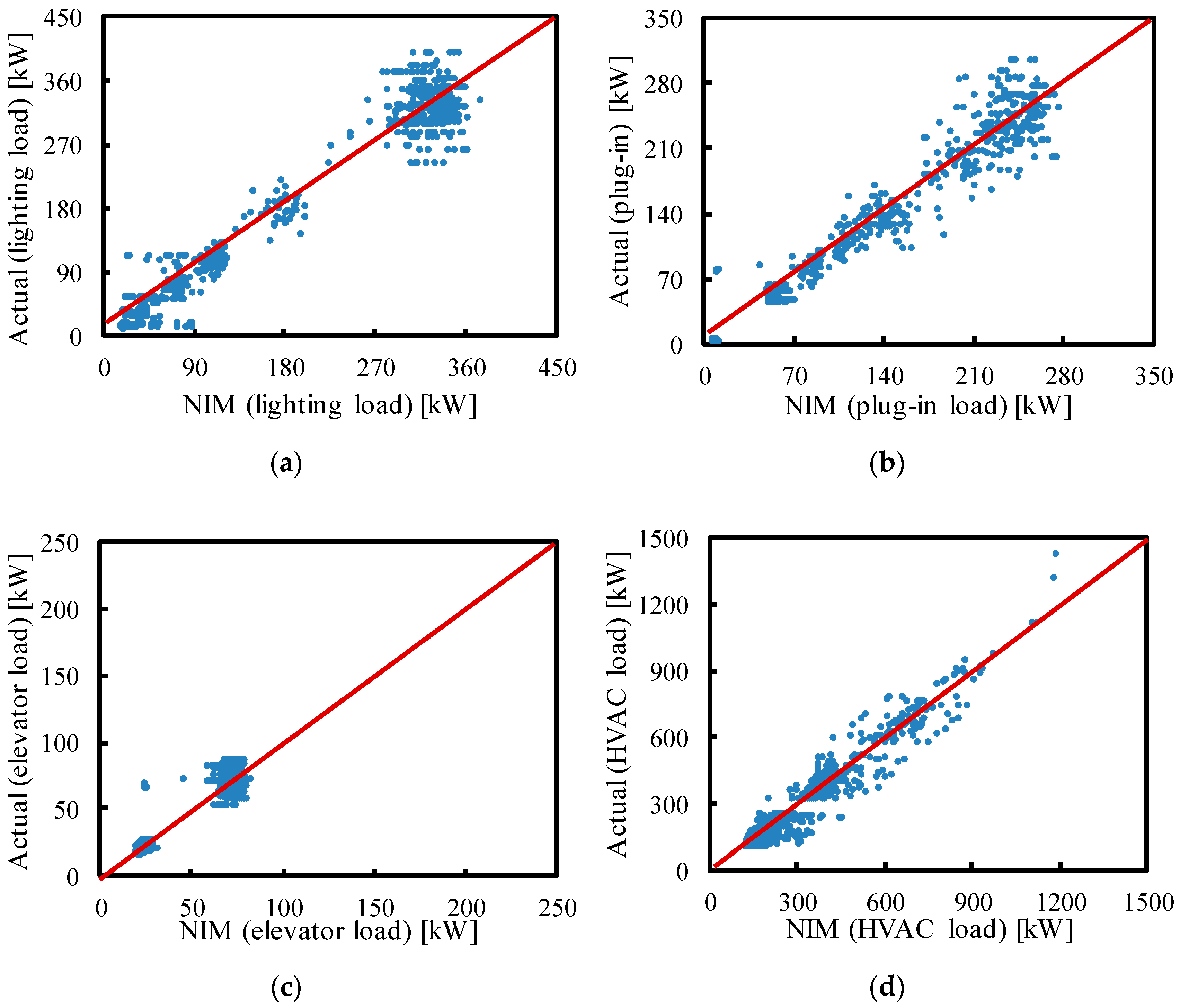
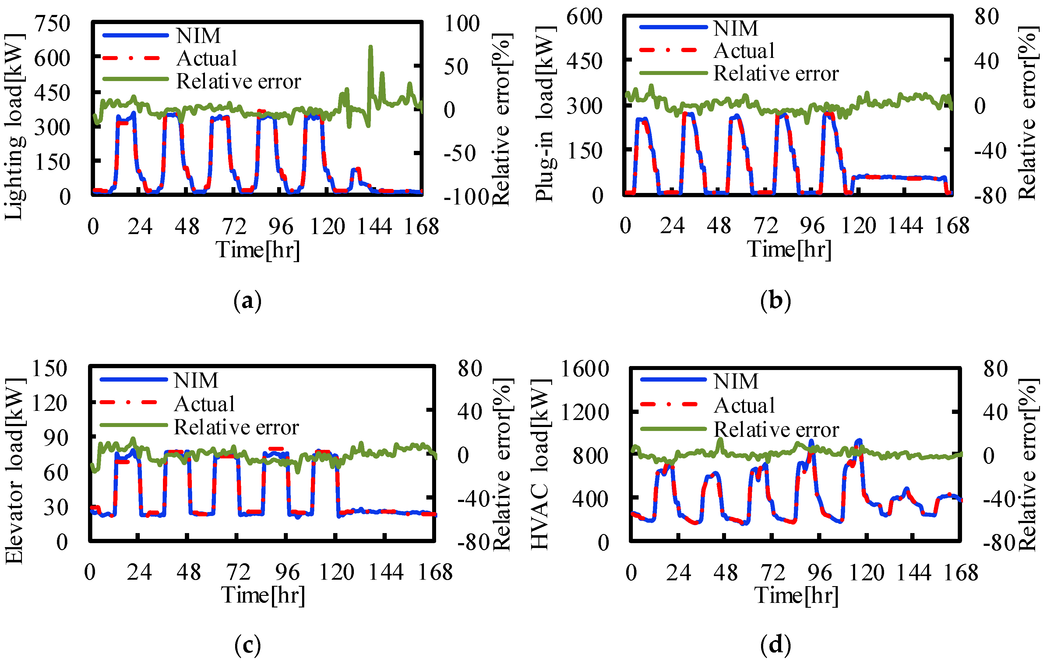
4.1. Disaggregation Results Based on Approach I

The training and testing results of the NIM model based on Approach I are shown in

Table 3. Training and testing results of NIM models based on Approach I.

Item	Training Results		Testing Results
	RMSE (kW)	MRE (%)	RMSE (kW)	MRE (%)
Lighting	4.4	3.4	16.8	11.0
Plug-in	4.0	3.0	12.7	8.2
Elevator	1.3	2.3	4.4	7.2
HVAC	7.8	1.3	28.8	7.1

. The approach takes the total energy consumption, dry-bulb temperature, relative humidity, and the time and days of the week as the inputs. The RMSEs and MREs of the training results of the four disaggregated subsystem loads range between 1.3 kW and 7.8 kW, and 1.3% and 3.4%, respectively. The RMSEs and MREs of the testing results of the four disaggregated subsystem loads range between 4.4 kW and 28.8 kW, and 7.1% and 11.0%, respectively. The results imply that the approach can accurately disaggregate the total energy consumption. For the four subsystems, the disaggregation results of the HVAC system load have the highest accuracy, followed by the elevator system load, plug-in system load, and lighting system load. The high accuracy of the disaggregation results of the HVAC system load is attributed to the strong correlation between the climate parameters and the HVAC system load, which enhances the mapping capability of the model.

The comparison between the calculated loads from the software and the disaggregation results was analyzed. The calculation loads were marked as Actual load, while the disaggregation loads were marked as NIM load. The test results for the whole test set are shown in Figure 5. Overall, most of the points evenly distribute on both sides of the line y = x, which indicates that the disaggregation results obtained by Approach I are accurate. Among the four types of subsystem loads, the disaggregation results of the lighting system and elevator system loads mainly concentrate on both ends of the line, while the disaggregation results of the plug-in system and HVAC system loads evenly concentrate on the whole line. This indicates that the lighting system and elevator system loads mainly consist of two types of high and low load levels, while the plug-in system and HVAC system loads have more states.

The test results for a typical week (Figure 6) show that the disaggregation results closely follow the actual loads, with limited absolute differences between them in most cases. Large differences mainly result from a sharp change in loads, such as the start and end of working hours. For the lighting system, plug-in system, elevator system, and HVAC system loads, most of the relative differences range between −5.69% and 6.90%, −7.32% and 5.04%, −6.51% and 4.81%, and −1.64% and 6.94%, respectively. Most of the relative differences are less than 8%, which indicates that the NIM models based on Approach I can obtain the subloads accurately. Figure 6 shows that the MREs can be large in some cases (i.e., the start or end of work) because the absolute values of these loads are very low, and small deviations lead to large relative errors.

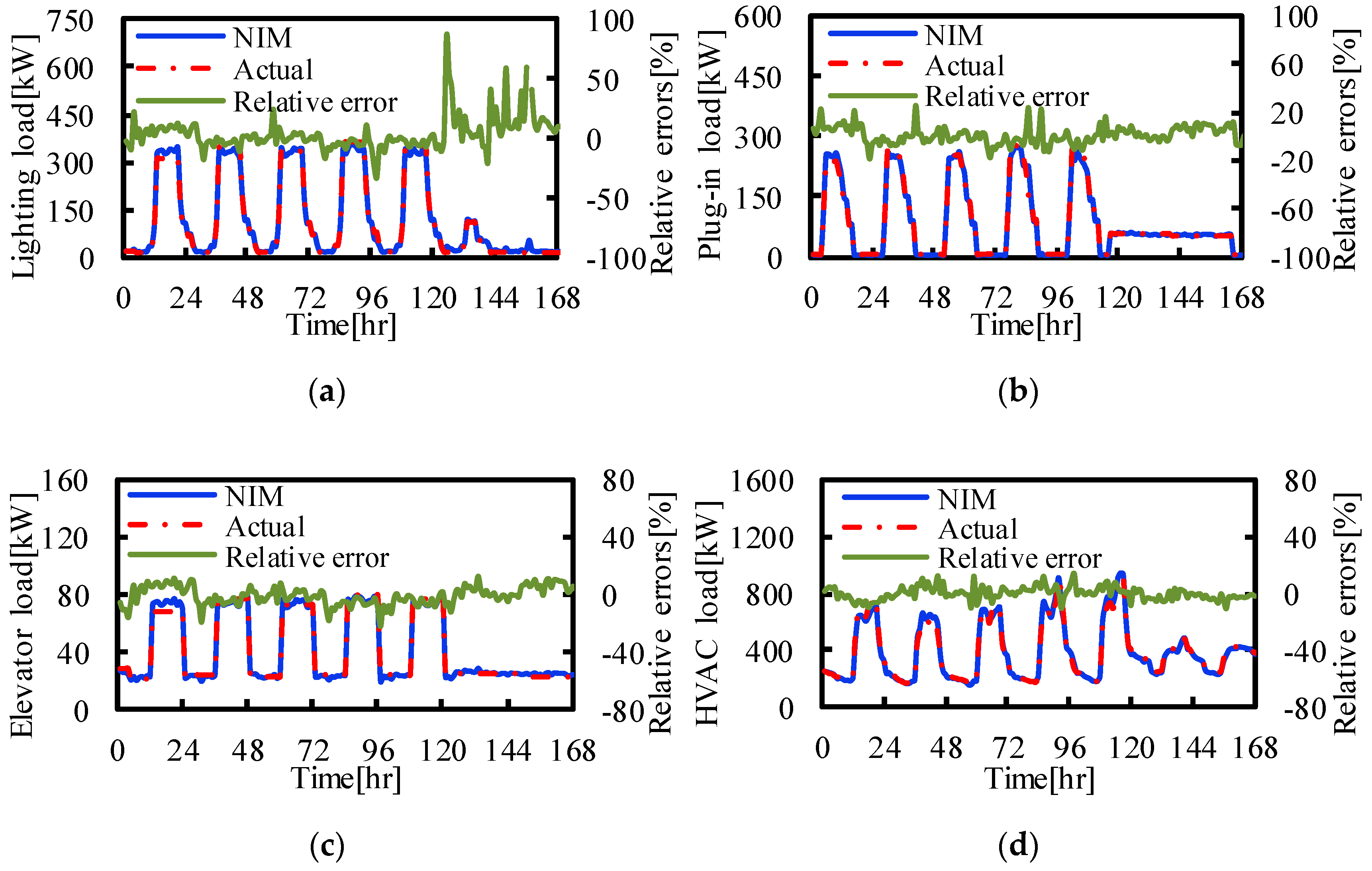
4.2. Disaggregation Results Based on Approach II

The training and testing results of the NIM models based on Approach II are presented in

Table 4. Training and testing results of NIM models based on Approach II.

Item	Training Results		Testing Results
	RMSE (kW)	MRE (%)	RMSE (kW)	MRE (%)
Lighting	7.1	5.0	24.0	12.7
Plug-in	4.9	4.0	16.5	10.1
Elevator	1.8	3.1	5.5	8.8
HVAC	13.5	2.3	46.2	12.1

. The approach applies the low-frequency and high-frequency coefficients from the disaggregated total energy consumption, the time, and the days of the week as inputs. The RMSEs and MREs of the training results of the four disaggregated subsystem loads range between 1.8 kW and 13.5 kW, and 2.3% and 5.0%, respectively. The RMSEs and MREs of the testing results of the four disaggregated subsystem loads range between 5.5 kW and 46.2 kW, and 8.8% and 12.7%, respectively. These results indicate that the approach can achieve accurate load disaggregation of the total energy consumption. For the four subsystems, the disaggregation results of the elevator system load are the most accurate, followed by the plug-in system and HVAC system. The disaggregation results of the lighting system load are not as accurate as those of the others.

The comparison between the calculated loads from the software and the disaggregation results was analyzed. The test results for the whole test set are shown in Figure 7. There are differences in distribution between the disaggregation results and actual loads, although most of the points distribute on both sides of the line y = x, which indicates that Approach II can disaggregate energy consumption accurately. Overall, the disaggregation results of elevator system load are more concentrated than other subsystem loads with more accurate results. The possible reason is that the energy consumption patterns of the elevator system are easy, contributing to learning the mapping relationship.

The test results for a typical week are shown in Figure 8. The disaggregation results match well with the actual loads in most cases, with a small gap between them. A sharp change in load sometimes causes large errors. For the lighting system, plug-in system, elevator system, and HVAC system loads, most of the relative differences range between −7.41% and 8.88%, −8.25% and 7.30%, −7.80% and 6.57%, and −3.23% and 11.16%, respectively. Most of the relative differences are less than 12%, which demonstrates that the NIM models based on Approach II can disaggregate the building-level energy consumption accurately. Large relative errors mainly occur when the loads are low (i.e., weekends). These small deviations lead to large relative errors owing to the small real values.

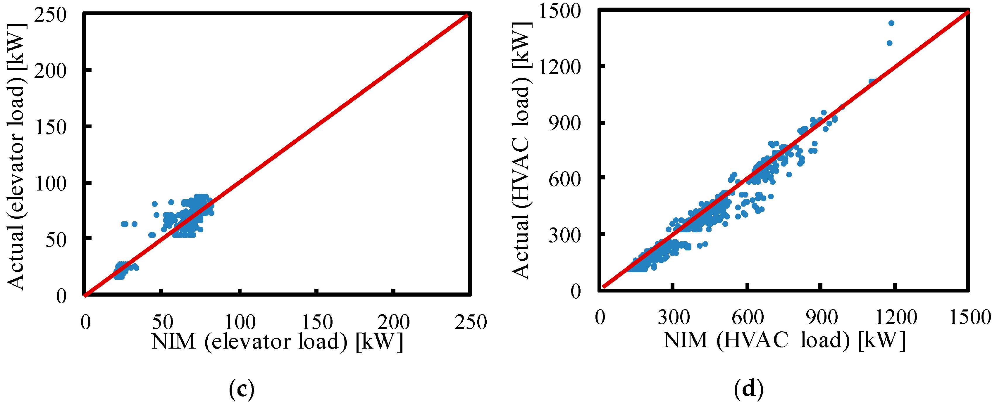
4.3. Disaggregation Results Based on Approach III

The training and testing results of the NIM models based on Approach III are shown in

Table 5. Training and testing results of NIM models based on Approach III.

Item	Training Results		Testing Results
	RMSE (kW)	MRE (%)	RMSE (kW)	MRE (%)
Lighting	5.5	3.6	25.0	11.9
Plug-in	3.8	2.7	16.8	9.8
Elevator	1.4	2.3	6.4	9.3
HVAC	10.3	1.7	46.4	11.4

. The approach employs new data transformed from daily energy consumption, time, and days of the week as the inputs. The RMSEs and MREs of the training results of the four disaggregated subsystem loads range between 1.4 kW and 10.3 kW, and 1.7% and 3.6%, respectively. The RMSEs and MREs of the testing results of the four disaggregated subsystem loads range between 6.4 kW and 46.4 kW, and 9.3% and 11.9%, respectively. The results indicate that the approach can disaggregate the total energy consumption accurately. For the four subsystem loads, the disaggregation results of the elevator system load are the most accurate, while those of the lighting system load have the lowest accuracy.

The comparison between the calculated loads from the software and the disaggregation results was analyzed. The test results for the whole test set are shown in Figure 9. Overall, most of the points evenly distribute on both sides of the line y = x and there are no obvious differences in distribution between the disaggregation results and actual loads. This indicates that the disaggregation results obtained by Approach III are accurate and the selected features are roughly suitable for the four types of subsystem loads.

The test results for a typical week in Figure 10 show that the disaggregation results and actual loads are well-matched in most cases, with limited absolute errors. Large errors mainly occur when the subsystem loads are at a high level. For the lighting system, plug-in system, elevator system, and HVAC loads, most of the relative differences range between −8.54% and 8.02%, −8.28% and 6.07%, −8.48% and 6.41%, and −3.22% and 9.68%, respectively. Most of the relative differences are less than 10%, which demonstrates that the NIM models based on Approach III can disaggregate the building-level energy consumption accurately. Large relative errors mainly occur when the loads are low (i.e., weekends). This is because the small deviations lead to large relative errors owing to the small real values.

4.4. Performance Comparison of the Three Approaches

The subsystem loads can be identified precisely by the NIM methods based on the three approaches. The performance of these three approaches is compared in

Table 6. Comparison of the MREs of testing results of the NIM models between Approach I and others.

Item	Difference of MRE between Approach I and Approach II (%)	Difference of MRE between Approach I and Approach III (%)
Lighting	−1.7	−0.9
Plug-in	−1.9	−1.6
Elevator	−1.6	−2.1
HVAC	−5	−4.3

and it indicates that the performance of Approach I is better than those of the other two approaches. One possible reason is that the outdoor weather variables are highly relevant features for the HVAC system load, which contributes to improving the accuracy of the overall disaggregation results. The dry-bulb temperature and relative humidity are considered in Approach I, and extra sensors for monitoring the two variables should be installed. Although the accuracy of the other two approaches is not as high as that of Approach I, they reduce the difficulty of data collection because only the total load is required. When weather data are inaccessible, the NIM methods based on Approach II and Approach III are recommended with acceptable accuracy.

Loads of the HVAC system, elevator system, plug-in system, and lighting system can be categorized as nonperiodic and periodic loads, which results in various performances for the three approaches. For periodic loads (loads of the elevator system, plug-in system, and lighting system), the differences in the accuracy of the three approaches are limited. The possible reason for this is that the characteristics selected in all three methods are similar to the correlations of these three types of loads. For the nonperiodic HVAC system load, Approach I outperforms Approach II and Approach III because outdoor weather variables, which are strongly related to the cooling loads of HVAC systems, are used as inputs in Approach I.

5. Conclusions

A NIM method based on RF was proposed to disaggregate the building-level energy consumption into the energy consumption of subsystems. Given the services provided by the buildings, four subsystem loads were disaggregated: loads of the HVAC system, elevator system, plug-in system, and lighting system. Three types of features were chosen to realize the NIM depending on the availability of weather data. By considering the case study of an office building, the following conclusions can be drawn:

• The proposed NIM method based on RF can achieve subsystem load disaggregation accurately. The RMSEs and MREs of the NIM results are less than 46.4 kW and 12.7%, respectively.
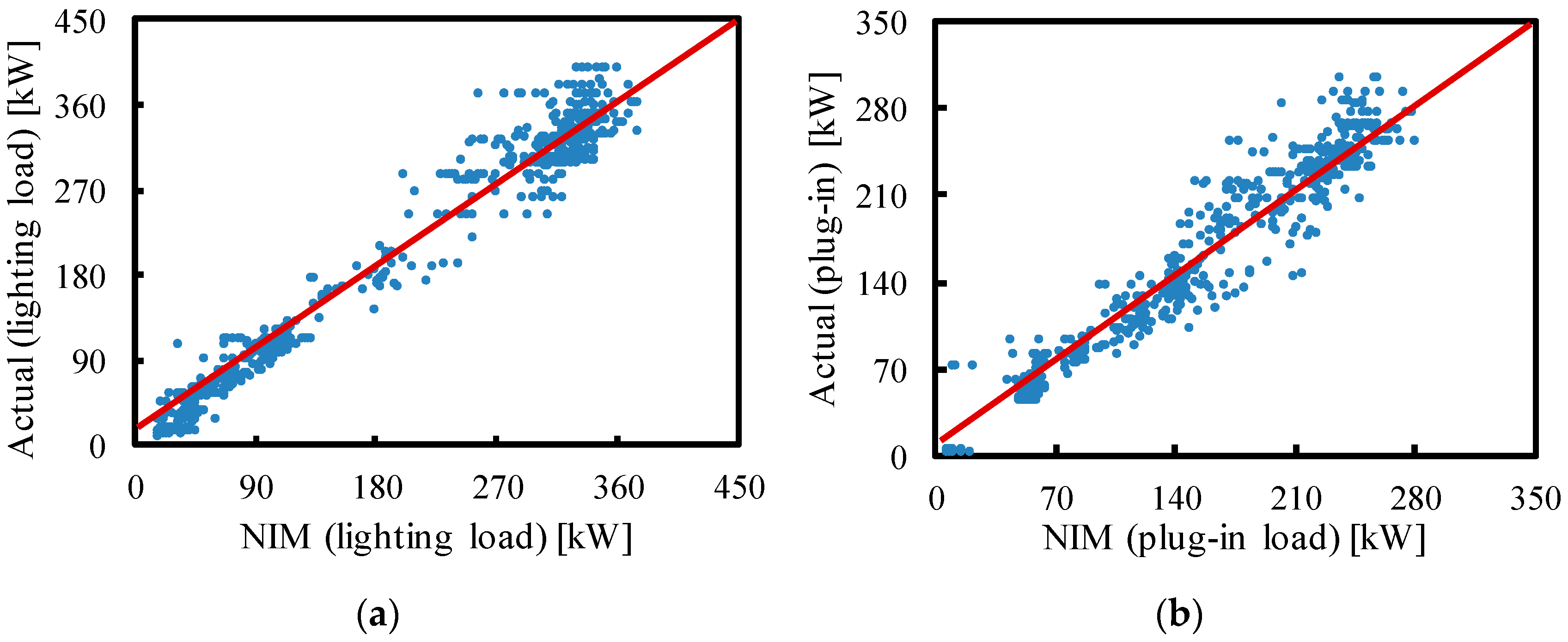
• All four subloads can be disaggregated with high accuracy. For the lighting system, plug-in system, elevator system, and HVAC system loads, the RMSEs (MREs) range from 16.8 kW to 25.0 kW (11.0% to 12.7%), 12.7 kW to 16.8 kW (8.2% to 10.1%), 4.4 kW to 6.4 kW (7.2% to 9.3%), and 28.8 kW to 46.4 kW (7.1% to 12.1%), respectively.
• The three proposed approaches can achieve subsystem load disaggregation accurately. When weather data are obtained, Approach I achieves the most accurate NIM results with RMSEs and MREs of less than 28.8 kW and 11.0%, respectively. When weather data are inaccessible, the NIM method based on Approach II and Approach III is recommended with acceptable accuracy, with RMSEs and MREs of less than 46.4 kW and 12.7%, respectively.
• For periodic loads (loads of the elevator system, plug-in system, and lighting system), the differences in the accuracy of the three approaches are small. For the nonperiodic HVAC system loads, Approach I outperforms Approach II and Approach III.

The proposed NIM method can perform the NIM of subsystem loads and it is based on supervised algorithms. The collection of training samples is significant for supervised algorithms. Obtaining the subsystem loads and the total load is a problem when the method is used. In addition, to promote the application of the NIM method, unsupervised methods without training the models should be developed, which would be addressed in the future study.

References

1. Fathi, S.; Srinivasan, R.; Fenner, A.; Fathi, S. Machine learning applications in urban building energy performance forecasting: A systematic review. Renew. Sustain. Energy Rev. 2020, 133, 110287. [Google Scholar] [CrossRef]
2. Pai, V.; Elzarka, H. Whole building life cycle assessment for buildings: A case study on how to achieve the LEED credit. J. Clean. Prod. 2021, 297, 126501. [Google Scholar] [CrossRef]
3. Zou, P.X.; Alam, M. Closing the building energy performance gap through component level analysis and stakeholder collaborations. Energy Build. 2020, 224, 110276. [Google Scholar] [CrossRef]
4. Fan, C.; Xiao, F.; Li, Z.; Wang, J. Unsupervised data analytics in mining big building operational data for energy efficiency enhancement: A review. Energy Build. 2018, 159, 296–308. [Google Scholar] [CrossRef]
5. Hernández, Á.; Ruano, A.; Ureña, J.; Ruano, M.; Garcia, J. Applications of NILM techniques to energy management and assisted living. IFAC-PapersOnLine 2019, 52, 164–171. [Google Scholar] [CrossRef]
6. Gunay, H.B.; Shi, Z.; Wilton, I.; Bursill, J. Disaggregation of commercial building end-uses with automation system data. Energy Build. 2020, 223, 110222. [Google Scholar] [CrossRef]
7. Aladesanmi, E.; Folly, K. Overview of non-intrusive load monitoring and identification techniques. IFAC-PapersOnLine 2015, 48, 415–420. [Google Scholar] [CrossRef]
8. Hamid, O.; Barbarosou, M.; Papageorgas, P.; Prekas, K.; Salame, C.-T. Automatic recognition of electric loads analyzing the characteristic parameters of the consumed electric power through a non-intrusive monitoring methodology. Energy Procedia 2017, 119, 742–751. [Google Scholar] [CrossRef]
9. Shi, X.; Ming, H.; Shakkottai, S.; Xie, L.; Yao, J. Nonintrusive load monitoring in residential households with low-resolution data. Appl. Energy 2019, 252, 113283. [Google Scholar] [CrossRef]
10. Bonfigli, R.; Principi, E.; Fagiani, M.; Severini, M.; Squartini, S.; Piazza, F. Non-intrusive load monitoring by using active and reactive power in additive factorial hidden Markov models. Appl. Energy 2017, 208, 1590–1607. [Google Scholar] [CrossRef]
11. Batra, N.; Parson, O.; Berges, M.; Singh, A.; Rogers, A. A comparison of non-intrusive load monitoring methods for commercial and residential buildings. arXiv 2014, arXiv:1408.6595. [Google Scholar]
12. Hart, G.W. Nonintrusive appliance load monitoring. Proc. IEEE 1992, 80, 1870–1891. [Google Scholar] [CrossRef]
13. Zhao, B.; Ye, M.; Stankovic, L.; Stankovic, V. Non-intrusive load disaggregation solutions for very low-rate smart meter data. Appl. Energy 2020, 268, 114949. [Google Scholar] [CrossRef]
14. Xia, M.; Liu, W.; Wang, K.; Zhang, X.; Xu, Y. Non-intrusive load disaggregation based on deep dilated residual network. Electr. Power Syst. Res. 2019, 170, 277–285. [Google Scholar] [CrossRef]
15. Wang, S.; Chen, H.; Guo, L.; Xu, D. Non-intrusive load identification based on the improved voltage-current trajectory with discrete color encoding background and deep-forest classifier. Energy Build. 2021, 244, 111043. [Google Scholar] [CrossRef]
16. Biansoongnern, S.; Plangklang, B. Nonintrusive load monitoring (NILM) using an Artificial neural network in embedded system with low sampling rate. In Proceedings of the 13th International Conference on Electrical Engineering/Electronics, Computer, Telecommunications and Information Technology (ECTI-CON), Chiang Mai, Thailand, 28 June–1 July 2016; pp. 1–4. [Google Scholar]
17. Himeur, Y.; Alsalemi, A.; Bensaali, F.; Amira, A. Effective non-intrusive load monitoring of buildings based on a novel multi-descriptor fusion with dimensionality reduction. Appl. Energy 2020, 279, 115872. [Google Scholar] [CrossRef]
18. Zhang, Y.; Yang, G.; Ma, S. Non-intrusive load monitoring based on convolutional neural network with differential input. Procedia CIRP 2019, 83, 670–674. [Google Scholar] [CrossRef]
19. Welikala, S.; Thelasingha, N.; Akram, M.; Ekanayake, P.B.; Godaliyadda, R.I.; Ekanayake, J.B. Implementation of a robust real-time non-intrusive load monitoring solution. Appl. Energy 2019, 238, 1519–1529. [Google Scholar] [CrossRef]
20. Cominola, A.; Giuliani, M.; Piga, D.; Castelletti, A.; Rizzoli, A. A Hybrid signature-based iterative Disaggregation algorithm for non-intrusive load monitoring. Appl. Energy 2017, 185, 331–344. [Google Scholar] [CrossRef]
21. Wang, J.; Hou, J.; Chen, J.; Fu, Q.; Huang, G. Data mining approach for improving the optimal control of HVAC systems: An event-driven strategy. J. Build. Eng. 2021, 39, 102246. [Google Scholar] [CrossRef]
22. Wagiman, K.R.; Abdullah, M.N.; Hassan, M.Y.; Radzi, N.H.M.; Abu Bakar, A.H.; Kwang, T.C. Lighting system control techniques in commercial buildings: Current trends and future directions. J. Build. Eng. 2020, 31, 101342. [Google Scholar] [CrossRef]
23. Norford, L.K.; Leeb, S.B. Non-intrusive electrical load monitoring in commercial buildings based on steady-state and transient load-detection algorithms. Energy Build. 1996, 24, 51–64. [Google Scholar] [CrossRef]
24. Wang, Y.; Pandharipande, A.; Fuhrmann, P. Energy data analytics for non-intrusive lighting asset monitoring and energy disaggregation. IEEE Sens. J. 2018, 18, 2934–2943. [Google Scholar] [CrossRef]
25. Jazizadeh, F.; Ahmadi-Karvigh, S.; Becerik-Gerber, B.; Soibelman, L. Spatiotemporal lighting load disaggregation using light intensity signal. Energy Build. 2014, 69, 572–583. [Google Scholar] [CrossRef]
26. Ying, J.; Peng, X.; Ye, Y. HVAC terminal hourly end-use disaggregation in commercial buildings with Fourier series model. Energy Build. 2015, 97, 33–46. [Google Scholar]
27. Doherty, B.; Trenbath, K. Device-level plug load disaggregation in a zero energy office building and opportunities for energy savings. Energy Build. 2019, 204, 109480. [Google Scholar] [CrossRef]
28. Wang, Z.; Wang, Y.; Zeng, R.; Srinivasan, R.; Ahrentzen, S. Random Forest based hourly building energy prediction. Energy Build. 2018, 171, 11–25. [Google Scholar] [CrossRef]
29. Makariou, D.; Barrieu, P.; Chen, Y. A random forest based approach for predicting spreads in the primary catastrophe bond market. Insur. Math. Econ. 2021. [Google Scholar] [CrossRef]
30. Mohana, R.M.; Reddy, C.K.K.; Anisha, P.; Murthy, B.R. Random Forest Algorithms for the Classification of Tree-Based Ensemble; Elsevier: Amsterdam, The Netherlands, 2021. [Google Scholar]
31. Zakariazadeh, A. Smart meter data classification using optimized random forest algorithm. ISA Trans. 2021. [Google Scholar] [CrossRef]
32. Lahouar, A.; Slama, J.B.H. Day-ahead load forecast using random forest and expert input selection. Energy Convers. Manag. 2015, 103, 1040–1051. [Google Scholar] [CrossRef]
33. Doucoure, B.; Agbossou, K.; Cardenas, A. Time series prediction using artificial wavelet neural network and multi-resolution analysis: Application to wind speed data. Renew. Energy 2016, 92, 202–211. [Google Scholar] [CrossRef]
34. Curceac, S.; Milne, A.; Atkinson, P.M.; Wu, L.; Harris, P. Elucidating the performance of hybrid models for predicting extreme water flow events through variography and wavelet analyses. J. Hydrol. 2021, 598, 126442. [Google Scholar] [CrossRef]
35. Bashir, Z.A.; El-Hawary, M.E. Applying wavelets to short-term load forecasting using PSO-based neural networks. IEEE Trans. Power Syst. 2009, 24, 20–27. [Google Scholar] [CrossRef]
36. Sun, Y.; Haghighat, F.; Fung, B.C. A review of the-state-of-the-art in data-driven approaches for building energy prediction. Energy Build. 2020, 221, 110022. [Google Scholar] [CrossRef]
37. Farrugia, J.; Griffin, S.; Valdramidis, V.P.; Camilleri, K.; Falzon, O. Principal component analysis of hyperspectral data for early detection of mould in cheeselets. Curr. Res. Food Sci. 2021, 4, 18–27. [Google Scholar] [CrossRef]
38. Pedregosa, F.; Varoquaux, G.; Gramfort, A.; Michel, V.; Thirion, B.; Grisel, O.; Blondel, M.; Müller, A.; Nothman, J.; Louppe, G. Scikit-learn: Machine Learning in Python. J. Mach. Learn. Res. 2012, 12, 2825–2830. [Google Scholar]
39. Rao, C.; Liu, M.; Goh, M.; Wen, J. 2-stage modified random forest model for credit risk assessment of P2P network lending to “Three Rurals” borrowers. Appl. Soft Comput. 2020, 95, 106570. [Google Scholar] [CrossRef]
40. Nadi, A.; Moradi, H. Increasing the views and reducing the depth in random forest. Expert Syst. Appl. 2019, 138, 112801. [Google Scholar] [CrossRef]
41. Qu, Z.; Xu, J.; Wang, Z.; Chi, R.; Liu, H. Prediction of electricity generation from a combined cycle power plant based on a stacking ensemble and its hyperparameter optimization with a grid-search method. Energy 2021, 227, 120309. [Google Scholar] [CrossRef]
42. MOHURD. Design Standard for Energy Efficiency of Public Buildings GB50189; Ministry of Housing and Urban-Rural Development of the China: Beijing, China, 2015.
43. Canada Institute. Practical Heating and Air Conditioning Design Manual, 2nd ed.; Canada Institute: Washington, DC, USA, 2010. [Google Scholar]
44. Zhao, J.; Lasternas, B.; Lam, K.P.; Yun, R.; Loftness, V. Occupant behavior and schedule modeling for building energy simulation through office appliance power consumption data mining. Energy Build. 2014, 82, 341–355. [Google Scholar] [CrossRef]
45. Wu, W.; Li, X.; You, T.; Wang, B.; Shi, W. Hybrid ground source absorption heat pump in cold regions: Thermal balance keeping and borehole number reduction. Appl. Therm. Eng. 2015, 90, 322–334. [Google Scholar] [CrossRef]
Figure 1. The framework of the NIM method based on RF.
Buildings 11 00449 g001
Figure 2. The physical model of the building in Google Sketchup.
Buildings 11 00449 g002
Figure 3. Annual hourly energy consumption of the building.
Buildings 11 00449 g003
Figure 4. The total loads and loads of four types of subsystems in a typical week for (a) summer and (b) winter.
Buildings 11 00449 g004
Figure 5. Testing results of the NIM model based on Approach I: (a) the comparison results of lighting system load; (b) the comparison results of plug-in system load; (c) the comparison results of elevator system load; (d) the comparison results of HVAC system load.
Buildings 11 00449 g005aBuildings 11 00449 g005b
Figure 6. Testing results of the NIM model based on Approach I in a typical week: (a) the comparison results of lighting system load; (b) the comparison results of plug-in system load; (c) the comparison results of elevator system load; (d) the comparison results of HVAC system load.
Buildings 11 00449 g006
Figure 7. Testing results of the NIM model based on Approach II: (a) the comparison results of lighting system load; (b) the comparison results of plug-in system load; (c) the comparison results of elevator system load; (d) the comparison results of HVAC system load.
Buildings 11 00449 g007aBuildings 11 00449 g007b
Figure 8. Testing results of the NIM model based on Approach II in a typical week: (a) the comparison results of lighting system load; (b) the comparison results of plug-in system load; (c) the comparison results of elevator system load; (d) the comparison results of HVAC system load.
Buildings 11 00449 g008
Figure 9. Testing results of the NIM model based on Approach III: (a) the comparison results of lighting system load; (b) the comparison results of plug-in system load; (c) the comparison results of elevator system load; (d) the comparison results of HVAC system load.
Buildings 11 00449 g009
Figure 10. Testing results of the NIM model based on Approach III in a typical week: (a) the comparison results of lighting system load; (b) the comparison results of plug-in system load; (c) the comparison results of elevator system load; (d) the comparison results of HVAC system load.
Buildings 11 00449 g010