Article

Analysis of Laser Tracker-Based Volumetric Error Mapping Strategies for Large Machine Tools

by
Beñat Iñigo
1,*,
Ander Ibabe
1,
Gorka Aguirre
1,
Harkaitz Urreta
1 and
Luis Norberto López de Lacalle
2
1
Design and Precision Engineering Group, IDEKO, 20870 Elgoibar, Spain
2
Department of Mechanical Engineering, EHU-UPV, 48013 Bilbao, Spain
*
Author to whom correspondence should be addressed.
Metals 2019, 9(7), 757; https://doi.org/10.3390/met9070757
Submission received: 28 May 2019 / Revised: 1 July 2019 / Accepted: 3 July 2019 / Published: 5 July 2019
(This article belongs to the Special Issue New Processes and Machine Tools for Advanced Metal Alloys)

Abstract

:
The measurement and compensation of volumetric error in milling machines of medium and large size is a key aspect to meeting the precision requirements of the most demanding applications. There are several solutions for volumetric error measurement—usually based on laser or in calibrated artifacts—that offer different specifications and lead to a variety of levels of precision, complexity of implementation and automation, cost of equipment, and measurement time, amongst others. Therefore, it is essential to have tools that allow, in each case, analysis as to which is the optimal calibration strategy, providing the criteria for evaluating different measurement equipment and strategies. To respond to this need, several tools have been developed which are able to simulate the entire calibration and compensation process (machine, measurement, model adjustment, etc.) and apply optimization methods to find the best measurement strategy for each application. For a given machine architecture and expected error ranges, the compensation error for each strategy is obtained by propagating measurement uncertainties and expected machine errors through the measurement and compensation model fitting process by Monte Carlo simulations. The use of this tool will be demonstrated through the analysis of the influence of the main design parameters of a measurement strategy for the calibration of a 3-axis machine tool, based on the measurement of tool position with a laser tracker.

1. Introduction

Geometric errors are one of the most important aspects when evaluating the precision of a machine tool. The form and assembly errors of the components of the machine (guideways, spindles, linear encoders, etc.) affect the position of the tool center point (TCP), causing a volumetric error that varies according to the position of the axes of the machine [1,2].
Traditionally, these errors have been measured by means of the so-called direct methods, measuring the error components of each axis (positioning, straightness, orientation) and their relative orientation (perpendicularity, parallelism) individually, to then compensate mechanically or by numerical control. Due to the high cost in time and the difficulties of measuring some errors individually, the so-called indirect methods have been developed in recent years. These procedures, usually based on calibrated artifacts [3] or laser interferometry with tracking (laser trackers) [4], directly measure the deviations of the TCP in different positions of the working volume and analytically infer the geometric errors that cause such deviations. In this way, a model is obtained that can be extrapolated to other points in the workspace, thus performing a complete volumetric calibration by means of a single procedure.
The earlier procedures for volumetric calibration have been based on the measurement of calibrated artifacts with different shapes and patterns [5,6,7,8], comparing the distances measured in the machine with the ones previously calibrated. These methods are well-suited to small- and medium-sized machines, but they have limitations when measuring larger volumes due to their limited size and the need for tools for their handling and positioning [9].
In recent years, volumetric calibration procedures have been developed based on the use of laser trackers (LTs). On the one hand, there are methods that only use distance measurement of the laser interferometer of the device [10,11,12], in which the distance from the LT to the TCP is measured from different positions and the 3D position of the point is obtained by multilateration. This technique has been used for demanding applications in small- and medium-sized machines, but loses its effectiveness in very large volumes [13]. On the other hand, the 3D position of the TCP can be measured by the usual application of the LT, which uses the interferometer and two angular encoders to locate the point in the working volume, and then tries to minimize the error between the measured and nominal position [14,15]. This approach can reduce the acquisition time, while facilitating data processing. Even so, it has traditionally been considered that, with the level of precision that commercial LTs can reach, this procedure is not suitable for high precision machines [8], where the magnitude of the errors to be calibrated can be below 0.01 mm.
Regardless of the measurement method used, each process needs to be optimized and validated to ensure the best possible results. There are many variables and aspects to consider when designing a calibration procedure: choice of equipment to be used, strategy of points to measure, optimization of trajectories, mathematical model, etc. In addition to this, it is necessary to validate the procedure to see if the desired results are obtained. Carrying out this process with in-machine tests and real equipment can be extremely costly both in terms of time and the economic aspect, as most of the time it can be impossible to achieve automated planning to minimize the uncertainty of machine tool calibration.
The simulation tools presented here offer a great advantage in these cases, allowing for the analysis of different measurement devices and strategies, propagation of uncertainties and expected machine errors, and validation of the complete process in a reduced amount of time. Several virtual tools have been previously proposed to try to forecast specific behaviors of the calibration process [16] or to obtain measurement uncertainties using the Monte Carlo method [17].
This article presents a novel optimization and virtual validation procedure of a complete process of calibration and volumetric compensation for a large milling machine, using conventional laser tracker as a measuring instrument. The whole virtual calibration process (virtual measurement, parameter estimation algorithm and validation process) is included in a Monte Carlo loop, and different design parameters are evaluated according to the output of this simulations.

2. Materials and Methods

2.1. Virtual Calibration and Compensation

The calibration process consists of measuring the position of the TCP along several positions of the working volume with the laser tracker. At each point, the 3D position measured by the LT (API, Rockville, MD, USA) and the nominal axes position will be recorded, and there will be differences between them due to both the geometric errors of the machine itself and the measurement uncertainties of the laser tracker. The deviation recorded between both measurements will be used to adjust and obtain a mathematical model that allows for the compensation of errors in the whole volume (see Section 2.3). The quality of the compensation and the obtained improvement in the volumetric error will depend on the proportion between the geometric errors of the machine tool and the uncertainties of the LT. To be able to simulate the calibration process virtually, it is necessary to define several aspects:
  • Structure and dimensions of the virtual machine tool, in addition to the shape and magnitude of the geometric errors.
  • Modeling of the laser tracker and characterization of the sources of uncertainty in the measurement process.
  • Definition of the measurement strategy: Type of trajectory, number of measurement points, LT positioning, etc.
  • Estimation of the compensation model: Choice of the mathematical algorithm, order of the adjustment model, type of polynomials to be used, etc.
  • Validation of results: Evaluating the improvement in accuracy after applying the compensation model obtained in the parameter estimation process.
An important aspect to keep in mind in these analyses is that in real calibrations, the geometric errors of the machine are not known a priori. These errors can vary in magnitude and form for different machines, and what can be a correct strategy for one case, may not be the right one for another. Therefore, it is necessary to consider this variability and to use the prior knowledge of the researcher for good modeling of these errors.
To estimate the uncertainty or accuracy level of a whole calibration plan is not straightforward, and several methodologies have recently been proposed [18]. To make an adequate comparison between different design alternatives, the calibration procedure is presented as an uncertainty propagation calculus, where the geometric errors represent the main input quantities (XM) along with the measurement uncertainties of LT (XLT). The volumetric error (whose quantification is defined in Section 2.4) will be the output quantity Y. Therefore, the analysis is not carried out on a single machine with specific geometrical errors, since the results of a single case may not be representative of the whole set. Instead, a Monte Carlo simulation will be carried out for each case study:
Ym = fm (XM, XLT),
where fm represents the whole calibration procedure and Ym represents the volumetric error distribution for case study m. This way, several virtual machines with different geometrical errors will be generated according to a set of parameters (see Section 2.2) and this case will be evaluated considering the distribution composed by the totality of the results of the simulated cases. To define the number of simulations required in each case, the Monte Carlo simulation will be performed iteratively according to Guide to the Expression of Uncertainty in Measurement (GUM) supplement 1 [19], in which the stabilization of the results will be evaluated. A diagram of the entire process, described above, can be seen in Figure 1.
The upper part of Figure 1 represents a single calibration and compensation procedure, performed in a specific machine by a LT, obtaining a compensation model with a parameter identification algorithm and evaluating the improvement of the volumetric error in a validation process. Several design parameters will be defined for each case study, and the whole procedure will be simulated N times in each. Output distribution will be used to compare different cases.

2.2. Modeling

A virtual volumetric calibration of a large gantry type milling machine will be carried out as an application example, whose schematic representation can be seen in Figure 2. Spatial error measurement is an issue that has recently been addressed with new formulations based on homogeneous transformation matrices [7,20], in either multi-axis lathes or in milling machines. Therefore, the kinematic structure of the machine is modeled using transformation matrices [9]. This virtual machine model provides the coordinates of the TCP, taking into account the nominal movement of the axes, the tool offset, and any error source that may cause deviations, such as the effects of the geometric errors present in each axis of the machine or environmental effects and the flexible behavior of the structure. Two machine models will be needed to implement the virtual calibration procedure. One will be used to simulate the real machine M in the calibration procedure, where any effect previously mentioned can be simulated. The other represents the calibration model C, where only the effects that want to be identified will be included (geometric errors in this case), since the identification of further effects will require a more extensive measurement procedure. Both machine models are defined as
M = VM(X, t, EM),
C = VM(X, t, EC),
where M represents the machine model used to generate the calibration test, C is the calibration model whose parameters need to be estimated, X represents the nominal movement of the axes, t is the tool offset, and EM and EC contains the parameters associated with different error sources.
The modeling of the geometric errors present in model M will be carried out by means of a combination of Fourier series and ordinary polynomial terms of order 0 and 1 [5]:
ENN (x) = a0 + a1 · x + ∑n (bn · sin(nπ · x) + cn · cos(nπ · x)),
where a0 and a1 are the 0 and 1 order terms of an ordinary polynomial, n is the order of the Fourier series terms, bn and cn are the sine and cosine amplitudes of nth Fourier term, and x represents the normalized position of the axis. With this equation, each of the 18 position-dependent geometric errors contained in a three-axis machine will be modeled [21].
As discussed in Section 2, the analysis of each case study is based on the results of several simulations. In each of them the geometric errors will be randomly generated, assigning a value according to a uniform distribution to the parameters of Equation (3). Parameters representing the amplitude (half-width) of the range for each error are described in Table 1.
The parameter set EC defined in model C will represented the geometric errors that will be identified in the parameter estimation procedure. The modeling of these geometric errors will be carried out by the combination of Legendre polynomials of grade 6, where each error be modeled as
ENN (x) = a0 · L0(x) + a1 · L1(x) + … + a6 · L6(x),
where the parameters an are the parameter to be estimated and Ln the Legendre polynomials of degree n.
The specifications of the virtual machine are summarized in Table 2, which remain the same for both M and C machine model.
The measurement process will be simulated by modeling a conventional laser tracker, consisting of a laser interferometer and two articulations controlled by angular encoders. The kinematic structure of the LT is also modeled by homogeneous transformation matrices. The virtual model was based on the commercial LT API Radian Pro® [24], in which it is considered that the systematic errors have been corrected:
LT = RTXYZ0 · RAZ · REL · TL,
where TL is the transformation matrix representing the laser interferometer measurement, and REL and RAZ are the rotation matrices for azimuth and elevation articulations of the laser tracker. RTXYZ0 represents the translation and rotation between the machine coordinate system and the LT, which is obtained a posteriori, fitting the coordinates measured by the LT with those recorded by the virtual machine.
The base and distance-dependent uncertainties of the encoders and the length measurement of the laser interferometer are modeled. To obtain the values of these parameters, a fitting process has been carried out simulating the in-line distance and horizontal scale bar measurements described in ASME B89.4.19 [25], and fitting the results with the ones provided by the LT manufacturer [24]. The fitting results for both tests can be seen in Figure 3.
Notable fitting has been achieved as both manufacturer data and model uncertainty values deviate less than 5 µm for the horizontal bar test and inside 1 µm in the in-line test, even for very large distances. Therefore, it is considered that the LT has been modeled with a sufficient level of accuracy.
Parameter values obtained in the previous procedure are shown in Table 3, where the uncertainty parameters are given for a coverage factor k = 1, assuming Gaussian distribution, as well as the range for the interferometer and the angular joints. No base uncertainty has been considered for distance measurement as the device will be used in the interferometer mode (IFM) and not as an absolute distance meter (ADM).

2.3. Parameter Estimation

Once the virtual calibration test has been generated, it is necessary to implement an estimation procedure that takes the recorded deviations as a starting point and tries to minimize them by adjusting the results to a model. In this case, the compensation model is a virtual machine similar to the one used in the generation of the test in which the 18 geometrical errors of a three-axis machine are parameterized in order to adjust to the measured errors. However, there are important differences regarding the machine used in the generation of the virtual calibration.
The polynomials used in the parameter estimation process are Legendre polynomials, which differ from those used when modeling the geometric errors of the original machine (see Equation (4)). In real machines, the geometric errors will never perfectly follow the shape of a specific polynomial form, so this modification is introduced to take into account the difference between the errors of the machine and those characterized in the compensation model.
These differences between the compensation model and the original system are known as model uncertainties [26]. These uncertainties are inevitable in any estimation process on a real system, either because you can never model the whole system in detail or because the calibration test does not contain enough information to infer and adjust all the parameters associated with the error sources. The differences between the original machine and the compensation model in the virtual calibration and compensation process allow for evaluation of the robustness of the process. It is important to note that the obtention of the compensation model is insensitive to whether the recorded errors come from a real test on a machine or a virtual one, as is the case here.
The goal of the adjustment process is to find the parameters EC of the Legendre polynomials that represent the geometric errors, in order to minimize the error between the measured deviations and those predicted by the model, adjusting the mentioned polynomials to the error forms of the original system. That is, an estimation procedure will be carried out so that the error between the real model M and the compensation model C in measured points X is minimized:
e = M(X, t, EM) − C(X, t, EC),
where e represents the error in X, Y, and Z direction ( e X , e Y , e Z ) of each point measured in the calibration.
This estimation is achieved by weighted least squares, a variation of the generalized least squares in which each measure is assumed to be independent of the others (there is no correlation between them), but that heteroscedasticity is present, that is, the measured values have different variances [6,27]. The analytical expression of this procedure can be observed in Equations (7) and (8).
e = AEC,
EC = (A’ · W−1 · A)−1 · A’ · W−1 · e,
where X represents the linear relationship between parameters and measurement errors defined by the compensation model and W is the weight matrix that is calculated according to the uncertainty associated with each measurement. The matrix is the form adopted by the covariance matrix Ω when all measurements are independent, so that all the elements outside the main diagonal are 0 and the elements of the diagonal are the variances associated with each measurement point in the three directions (σ2x, σ2y, σ2z). The calculation of this variance is made by propagating uncertainties of the LT model described in Section 2.2.

2.4. Validation of the Compensation Model

To evaluate the quality of the model obtained, the improvement of the volumetric error in the whole working volume is checked. For this purpose, a three-dimensional mesh is defined with uniformly spaced points in X, Y, and Z, and the deviation from the nominal point caused by the geometric errors is evaluated, taking this value as the initial error. Next, the volumetric compensation in three directions is applied for each point, which is calculated according to the model obtained in the previous step, improving the existing volumetric error:
VE0 = ||M(X, t, EM) − M(X, t, 0)||,
VE = ||M(Xv, t, EM) − C(Xv, t, EC)||,
where VE0 represents the initial volumetric error compared with an ideal machine behavior and VE the volumetric error after compensation is applied in all Xv validation points. Equations (9) and (10) provide the volumetric error distribution for Xv point set. In this paper, the RMS value of this distribution will be taken as a numeric value that defines the quality of the compensation procedure. Regarding the Monte Carlo simulation presented in Equation (1), the RMS value obtained in each simulation represents the yr draw of output variable Y that will compound the distribution of results.
It is important to highlight that using virtual tools significantly facilitates the evaluation of the adjustment quality. In the case of a real test, after carrying out the calibration test and adjusting the data, it is necessary to make new measurements on the machine to observe the improvement, which may involve a time cost very similar to the one invested in the calibration phase. Furthermore, the very same measurement uncertainties present in the calibration test will probably affect the validation test, as the same procedure is usually used, distorting the results that are supposed to be validated. However, in the case of virtual simulations, the validation is practically instantaneous and is done without any additional source of uncertainty.

3. Results and Discussion

In this section, comparisons between different case studies will be shown, that will allow optimizing different aspects of the calibration and compensation process. The aspects analyzed are the following:
  • Comparison between different types of measurement strategies.
  • Variation of the spacing between measurement points.
  • Similar measurements placing the LT in different positions.

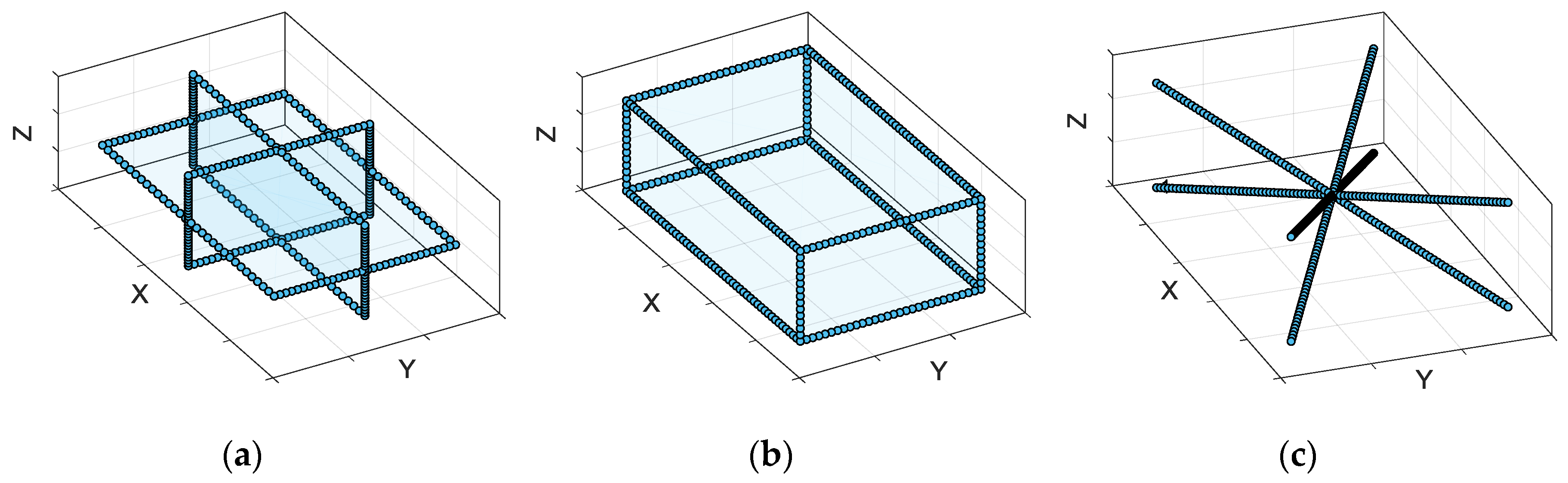
3.1. Measurement Trajectory Strategies

The first aspect to be analyzed is the path that the TCP should describe throughout the calibration process. The most common strategies consist of linear trajectories along the three linear axes in which the measurement of the TCP is registered at regular intervals. These trajectories are then combined to form planes, cubes, or other forms that encompass the entire working volume and provide enough information to infer the geometric errors.
In this comparison, three different measurement strategies have been studied: trajectories in the form of main planes, in the form of a hexahedron, and forming the main diagonals of the volume. These strategies can be observed in Figure 4. Due to the disparity of trajectories between the different strategies, the spacing between points of measurement has been adapted for each case, resulting in approximately the same total number of points and, therefore, in tests of comparable duration.
Simulation has been carried out according to the procedure shown in Section 2, Section 3 and Section 4. The results are shown in Figure 5, in which can be seen that the option of the plane-type trajectories is the one that provides the best results when it comes to improving the error in the volume. Therefore, in the successive analyses, it will be taken as the benchmark test to optimize the other aspects.

3.2. Spacing between Measurement Points

In this section, the improvement of volumetric error will be analyzed as the number of measured points increases (reducing the spacing between them) in the calibration test. The trajectory of the hexahedron presented in the previous section is used.
The results of the simulations are shown in Figure 6. The original volumetric error of the machine is compared with the error remaining after compensation for a growing number of measurements. The duration of the tests has been calculated by assigning 15 s to the measurement of each point and a fixed duration of 20 min to set the measurement system. As expected, as the number of points increases, the quality of the compensation improves, obtaining a substantial improvement at the beginning but stabilizing as the density increases. On the other hand, as the number of measurements increases, the duration of the test will also increase proportionally. Therefore, the decision on this point lies in deciding how long it is worthwhile to continue increasing the number of measurements considering the incremental improvement from one set to another.
Analyzing the results for this case, it could be said that above 600 points, the incremental improvement obtained would not compensate for the increase in the calibration time.
It is important to note that this tradeoff between duration and accuracy may vary depending on the application or the objectives of the calibration.

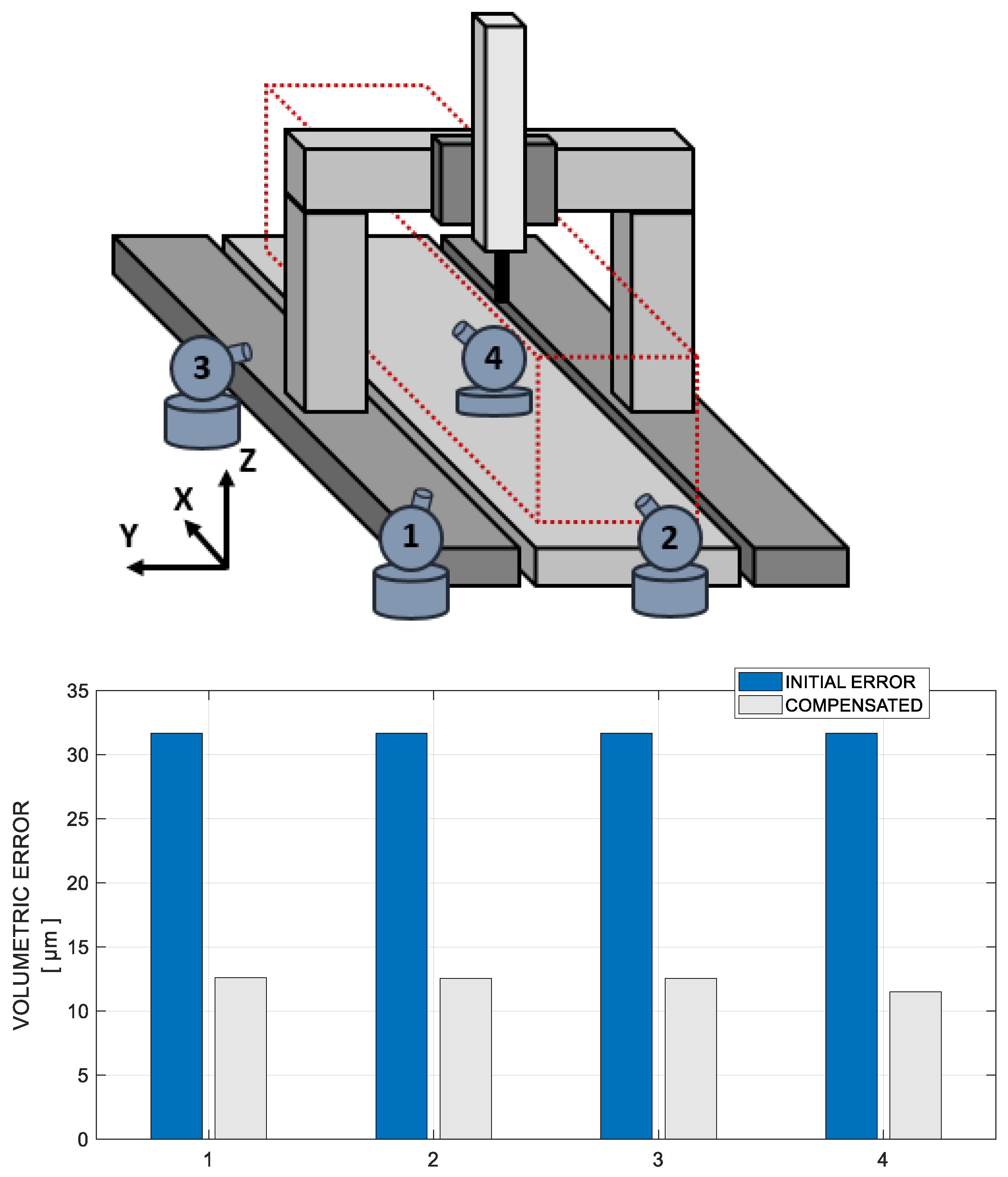
3.3. Positioning of Laser Tracker

The position of the LT with respect to the measurement points is another important aspect to consider when making the measurements. There are two main issues that must be taken into account when evaluating the position of the LT.
On the one hand, due to independent operation, the measurement uncertainty of the points furthest from the LT will always be greater because the accuracy of the interferometer decreases with distance, and the angular error of the encoders is also amplified (see Table 3). Therefore, the LT should be placed as close as possible to the set of points to be measured, including among the possibilities to place it within the volume itself.
On the other hand, there are several technical limitations regarding the possibility of measuring any point. Firstly, the articulation corresponding to the elevation angle has a limited range (see Table 3), limiting the possibilities to measure points strictly above the LT. Secondly, the reflector that reflects the laser beam, which is inserted in the position of the tool, usually has a limited angle of incidence (between 120° and 150°) that does not allow measuring in the most cornered positions. There are active reflectors with motorized axes that allow measurement from any angle, but equipment with such capabilities are limited and suppose a higher economic cost. Finally, there are mechanical limitations that depend on each case, in which, for example, the machine structure itself interferes with the measurements. For example, in Figure 7, the columns of the gantry machine would interfere to measure some points in position #3. In the simulations carried out in this section, these limitations of the structure itself will not be taken into account, as the correct evaluation of these effects would require virtual commissioning tools.
Figure 7 shows the simulated cases for this analysis. Position #1 is the most usual in this type of measurement, since it is the one that requires the lowest range of angle of incidence for the reflector. On the other hand, it is at the same time the furthest away from the measurement points. The positions #2 and #3 have a much more centered position, especially the #3, as it is located along the longer axis. However, these positions require greater amplitude to the reflector and may limit the measurement of some points. At this stage, it is necessary to decide between two alternatives:
  • Keep the LT in the same position, leaving the points out of range without measuring, hoping that a closer proximity to the other points will result in better characterization.
  • Move the LT slightly away in the opposite direction, measuring all the required points, but losing some precision due to the greater distance to the points.
In these analyses, the second option has been chosen. Position #4 is a special case since, to perform a measurement from there, it is absolutely necessary to have an active reflector. At the same time, it is the one with the least distance to the points set and, therefore, from which the best result could be expected. It is included in this analysis despite the limitations involved, to have it as a reference with respect to the other cases.
As can be seen in Figure 7, positions #1–#3 show very similar results. It is therefore considered that the effects mentioned in the previous paragraph are compensated to result in a similar calibration. Position #4 shows a slight improvement over the other positions as expected.

4. Discussion

Results obtained in Section 3 can be summarized in the following points:
  • Different trajectories in tests of similar duration affect the quality of the compensation. The orthogonal planes offer slightly better results than the hexahedron, which is the usual strategy in these types of calibrations.
  • Calibration quality shows an asymptotic behavior when tests with an increasing number of points are performed. When the number of measured points is high enough, stabilization of the improvement is reached.
  • The positioning points of the LT studied in this paper show minor influence in the quality of the calibration process. Centered position shows slightly better results, but an active reflector is required to measure all points.
In Section 3.1, the trajectory composed by the main diagonals shows the worst results. Further analysis has shown that the three axis movements used in this strategy makes it harder to decouple individual geometric errors, compared to multiple 1-axis linear trajectories, even if the total number of measurements remains the same. Regarding the results of orthogonal planes and hexahedron, similar results were expected, as both strategies represents similar trajectories in different configurations. The slightly better improvement in planes strategy is justified, as the mean distance from the measured points to LT position (position 1 in Figure 7) is smaller in this case.
In Section 3.2, it is important to note that the stabilization observed in Figure 6 as the number of points increases can vary according to the geometric errors of the machine. If the spatial frequencies of the errors are greater, it is expected that a greater density of points will be needed to characterize them correctly and, therefore, such stabilization will be achieved with a greater number of points. Further research on the relationship between measurement density, machine error order, and estimation model order is of major interest, in order to define an optimal measurement strategy and understand the influence of overfitting/underfitting.
In Section 3.3, the positions #1–#3 were shown to have minor influence regarding the final results. As the measurement strategies analyzed in this paper are symmetric, similar measurement distances from LT to TCP were achieved in each of the cases. Future research should be done analyzing the same effect in nonsymmetric measurement strategies. The improvement level for position #4 will depend on the distance-dependent accuracy of the LT. In such cases, using an active reflector should be considered.

5. Conclusions

This article has presented a new strategy for optimizing volumetric error calibration processes based on laser tracker by means of simulation of the whole calibration process. By following this approach, the goal is to be able to find the optimal calibration procedure for each machine to be compensated, which achieves the expected calibration accuracy with the minimal machine occupation time.
  • The feasibility and interest of the proposed approach have been demonstrated by performing an analysis of the calibration process on a large machine tool, which has provided meaningful results.
  • The calibration results obtained in the analyses indicate that laser trackers are a valid solution for the calibration of large machine tools but, also, that the measurement strategy can have a relevant influence on the calibration uncertainty and on the measurement time.
  • These resulting optimization criteria cannot be considered of general application, since the optimal solution for each machine type and customer requirements will lead to different solutions. What can be taken instead, as a general solution, is the methodology and simulation tools presented here for finding the optimal solution.
  • The simulation of the machine to be calibrated is critical for obtaining representative results, and requires an estimation of the expected machine errors. The proposed error modeling strategy and Monte Carlo simulation ensure that the required engineering judgement is properly considered in the optimization process.
  • The uncertainty model of the laser tracker, as considered in the product catalogue, has not been considered appropriate for the requirements of some of the analyses, such as the influence of the position of the laser tracker, and a model based on results of ASME B89.4.19 tests has been successfully implemented.

Author Contributions

Software and simulation design, A.I. and B.I.; methodology, G.A.; writing—original draft preparation, B.I.; supervision, G.A. and L.N.L.d.L.; project administration, H.U.

Funding

Thanks are due to funds from Excellence groups of the Basque university system n IT1337-19.

Conflicts of Interest

The authors declare no conflict of interest.

References

  1. Sartori, S.; Zhang, G. Geometric Error Measurement and Compensation of Machines. CIRP Ann. 1995, 44, 599–609. [Google Scholar] [CrossRef]
  2. Schwenke, H.; Knapp, W.; Haitjema, H.; Weckenmann, A.; Schmitt, R.; Delbressine, F. Geometric error measurement and compensation of machines—An update. CIRP Ann. 2008, 57, 660–675. [Google Scholar] [CrossRef]
  3. Cauchick-Miguel, P.; Kinga, T.; Davis, J. CMM verification: A survey. Measurement 1996, 17, 1–16. [Google Scholar] [CrossRef]
  4. Lau, K.; Hocken, R.; Haight, W. Automatic laser tracking interferometer system for robot metrology. Precis. Eng. 1986, 8, 3–8. [Google Scholar] [CrossRef]
  5. Bringmann, B. Improving Geometric Calibration Methods for Multi-Axis Machining Center by Examining Error Interdependencies Effects; ETH Zurich: Zurich, Switzerland, 2007; Available online: https://www.research-collection.ethz.ch/handle/20.500.11850/9153 (accessed on 15 May 2019).
  6. Díaz-Tena, E.; Ugalde, U.; De Lacalle, L.N.L.; De La Iglesia, A.; Calleja, A.; Campa, F.J.; De Lacalle, L.N.L. Propagation of assembly errors in multitasking machines by the homogenous matrix method. Int. J. Adv. Manuf. Technol. 2013, 68, 149–164. [Google Scholar] [CrossRef]
  7. Lamikiz, A.; De Lacalle, L.L.; Ocerin, O.; Díez, D.; Maidagan, E. The Denavit and Hartenberg approach applied to evaluate the consequences in the tool tip position of geometrical errors in five-axis milling centres. Int. J. Adv. Manuf. Technol. 2008, 37, 122–139. [Google Scholar] [CrossRef]
  8. Wang, J.D.; Guo, J.J.; Deng, Y.F.; Li, H.T. Method of Volumetric Error Compensation for 3-Axis NC Machine Tool. Adv. Mater. Res. 2012, 472, 2371–2376. [Google Scholar] [CrossRef]
  9. Ibaraki, S.; Knapp, W. Indirect Measurement of Volumetric Accuracy for Three-Axis and Five-Axis Machine Tools: A Review. Int. J. Autom. Technol. 2012, 6, 110–124. [Google Scholar] [CrossRef] [Green Version]
  10. Schwenke, H.; Franke, M.; Hannaford, J.; Kunzmann, H. Error mapping of CMMs and machine tools by a single tracking interferometer. CIRP Ann. 2005, 54, 475–478. [Google Scholar] [CrossRef]
  11. Zhang, Z.; Hu, H. Measurement and compensation of geometric errors of three-axis machine tool by using laser tracker based on a sequential multilateration scheme. Proc. Inst. Mech. Eng. Part B J. Eng. Manuf. 2014, 228, 819–831. [Google Scholar] [CrossRef]
  12. Mutilba, U.; Yagüe-Fabra, J.A.; Gomez-Acedo, E.; Kortaberria, G.; Olarra, A. Integrated multilateration for machine tool automatic verification. CIRP Ann. 2018, 67, 555–558. [Google Scholar] [CrossRef]
  13. Mutilba, U.; Gutierrez, A.; Olarra, A.; Kortaberria, G.; Gomez-Acedo, E. La Compensación Volumétrica de Los Errores geométricos en máquinas-herramienta, Interempresas. Available online: http://www.interempresas.net/MetalMecanica/Articulos/158159-La-compensacion-volumetrica-de-los-errores-geometricos-en-maquinas-herramienta.html (accessed on 15 May 2019).
  14. Wan, A.; Song, L.; Xu, J.; Liu, S.; Chen, K. Calibration and compensation of machine tool volumetric error using a laser tracker. Int. J. Mach. Tools Manuf. 2018, 124, 126–133. [Google Scholar] [CrossRef]
  15. Aguado, S.; Samper, D.; Santolaria, J.; Aguilar, J.J. Identification strategy of error parameter in volumetric error compensation of machine tool based on laser tracker measurements. Int. J. Mach. Tools Manuf. 2012, 53, 160–169. [Google Scholar] [CrossRef]
  16. Aguado, S.; Santolaria, J.; Samper, D.; Aguilar, J.J. Forecasting method in multilateration accuracy based on laser tracker measurement. Meas. Sci. Technol. 2016, 28, 25011. [Google Scholar] [CrossRef]
  17. Wang, H.; Shao, Z.; Fan, Z.; Han, Z. Configuration optimization of laser tracker stations for position measurement in error identification of heavy-duty machine tools. Meas. Sci. Technol. 2019, 30, 045009. [Google Scholar] [CrossRef]
  18. Parkinson, S.; Longstaff, A.; Fletcher, S.; Longstaff, A. Automated planning to minimise uncertainty of machine tool calibration. Eng. Appl. Artif. Intell. 2014, 30, 63–72. [Google Scholar] [CrossRef] [Green Version]
  19. JCGM. Evaluation of Measurement Data—Supplement 1 to the “Guide to the Expression of Uncertainty in Measurement”—Propagation of Distributions Using a Monte Carlo Method; JCGM: Sevres, France, 2008. [Google Scholar]
  20. Olvera, D.; De Lacalle, L.L.; Compeán, F.I.; Fz-Valdivielso, A.; Lamikiz, A.; Campa, F.J. Analysis of the tool tip radial stiffness of turn-milling centers. Int. J. Adv. Manuf. Technol. 2012, 60, 883–891. [Google Scholar] [CrossRef]
  21. ISO 230-1:2012. Test Code for Machine Tolos—Part 1: Geometric accuracy of Machines Operating under No-Load or Quasi-Static Conditions; ISO: Geneva, Switzerland, 2012. [Google Scholar]
  22. ISO 841:2001. Industrial Automation Systems and Integration—Numerical Control of Machines—Coordinate System and Motion Nomenclature; ISO: Geneva, Switzerland, 2001. [Google Scholar]
  23. ISO 10791-6:2014. Test Conditions for Machining Centres. Part 6: Accuracy of Feeds, Speeds, Interpolations; ISO: Geneva, Switzerland, 2014. [Google Scholar]
  24. API. API Radian 3D Laser Tracker Systems Brochure. Available online: https://apisensor.com/products/3d-laser-tracker-systems/radian/ (accessed on 15 May 2019).
  25. ASME. B89.4.19-2006 Performance Evaluation of Laser-Based Spherical Coordinate Measurement Systems; ASME: New York, NY, USA, 2006; Available online: https://www.asme.org/products/codes-standards/b89419-2006-performance-evaluation-laserbased (accessed on 15 May 2019).
  26. Morse, E.; Dantan, J.-Y.; Anwer, N.; Söderberg, R.; Moroni, G.; Qureshi, A.; Jiang, X.; Mathieu, L. Tolerancing: Managing uncertainty from conceptual design to final product. CIRP Ann. 2018, 67, 695–717. [Google Scholar] [CrossRef] [Green Version]
  27. Strutz, T. Data Fitting and Uncertainty: A Practical Introduction to Weighted Least Squares and Beyond, 2nd ed.; Springer: Berlin, Germany, 2016; Available online: https://www.springer.com/gp/book/9783658114558 (accessed on 15 May 2019).
Figure 1. Process diagram for the whole calibration and compensation procedure comparing several case studies.
Metals 09 00757 g001
Figure 2. Schematic representation of the kinematic chain of the virtual machine tool.
Metals 09 00757 g002
Figure 3. Model parameter fitting of the laser tracker (LT) to the manufacturer data for (a) horizontal scale bar test for angular measurement performance and (b) distance measurement performance.
Metals 09 00757 g003
Figure 4. Measuring trajectories to be compared: (a) Orthogonal planes; (b) Hexahedron; (c) Main diagonals.
Metals 09 00757 g004
Figure 5. Comparison of measured trajectories. Error distributions and mean values are shown, for values before (blue) and after (grey) compensation.
Metals 09 00757 g005
Figure 6. Simulation results with increasing measured points. Total number of points is shown, as well as the initial (blue) and compensated (grey) error.
Metals 09 00757 g006
Figure 7. Measurement process schematic view and compensation results for single position and two position measurements.
Metals 09 00757 g007
Table 1. Parameters used to generate the 18 geometric errors contained in a three-axis machine tool according to ISO 230.
Error ComponentsDistribution Parameters
a0a1n1b1c1n2b2c2
EXX0700.5202051010
EYX000.5300533
EZX000.5150533
EAX10200.51010555
EBX10200.51010555
ECX10200.51010555
EXY000.5150255
EYY0300.555233
EZY000.5150255
EAY10300.51010255
EBY10300.51010255
ECY10300.51010255
EXZ000.5150155
EYZ000.5150155
EZZ0300.53030133
EAZ10300.51010133
EBZ10300.51010133
ECZ10300.51010133
Table 2. Virtual machine specifications. Kinematic chain represented according to ISO 841 and ISO 10791-6 [22,23] (t: tool; b: bed; w: workpiece).
Machine ToolX (mm)Y (mm)Z (mm)
Working volume0–50000–30000–1500
Kinematic chaint–Z–Y–[X1 X2]–b–w
Table 3. Laser tracker model parameters with uncertainty values obtained from data fitting.
Laser TrackerRangeUncertainty (k = 1)
Laser Interferometer80 m-±0.25 µm/m
Azimuth±320°±10 µm±2.5 µm/m
Elevation(−59°, +79°)±10 µm±2.5 µm/m

