Some Facts We Can Learn from Analytical Modeling of DDRX in Pure Metals and Solid Solutions

Abstract

Modeling and simulation of discontinuous dynamic recrystallization (DDRX) are now commonly carried out by numerical methods, most often finite element computation. It is also possible to use simple analytical approaches on the grain scale to get relevant information about the basic mechanisms involved in DDRX, in particular regarding the large strain steady state behaviour. This is illustrated in the present paper on the basis of a model previously proposed by the author and co-workers, which is first briefly presented. The macroscopic constitutive parameters associated with DDRX are then derived and three distinct “Derby exponents” are introduced for describing the relationship between steady state grain size and flow stress. Finally, it is shown, with the example of grain sizes, that not only can average quantities be predicted analytically, but also their distributions.

1. Introduction

Dynamic recrystallization (DRX) plays a major role in thermomechanical processing of metals and alloys because it modifies their microstructures (first and foremost the grain size), flow stresses, and crystallographic textures. Two types of DRX can be distinguished: continuous dynamic recrystallization (CDRX) takes place in high stacking fault energy materials where dynamic recovery is very efficient. New grains are nucleated by the progressive generation of subgrain boundaries and the evolution of part of them into high angle boundaries. By contrast, discontinuous dynamic recrystallization (DDRX) occurs in low stacking fault energy metals: when dynamic recovery is weak, local concentrations of dislocations activate nucleation events, and large dislocation gradients induce large boundary migration rates. The DDRX microstructure then results from repeated cycles of nucleation, growth, shrinkage, and vanishing of grains. In both cases, if no fracture happens before, a self-organized steady state system arises at large strains, in equilibrium with the prescribed (constant) strain rate and temperature. Not only the average values of the material parameters (e.g., dislocation density, grain size) then remain constant upon further straining, but also their distributions.

Various approaches have been proposed for modeling DDRX in the past: after some analytical pioneering works [1,2], Monte Carlo calculations were published by Rollett and co-workers [3,4,5]. Several researchers used as an alternative cellular automata, although the latter are more adapted for describing static than dynamic recrystallization for strain has to be introduced in a somewhat artificial way [6,7], or by coupling the cellular automaton (for static recrystallization) with finite element computations (for deformation) [8]. More recently, the level set finite element technique has been introduced, which allows a full field description of the material during static [9] or dynamic [10] recrystallization. Such numerical computations provide the most detailed description of microstructural evolutions, but their ability to reach DDRX steady states, i.e., large to very large strains, is still questionable considering the current computing speeds. Finally, a new microscopic (and more ambitious) approach based on a thermodynamic theory of dislocation plasticity has been proposed [11,12] and applied to the interaction between DRX and adiabatic shear banding under high strain rate loading conditions. A review of DRX including modeling has been published recently by Huang and Logé [13].

In parallel with the above, a semi-analytical mesoscale (i.e., grain scale) approach has been proposed by Montheillet and co-workers [14,15], which starts from simple physical assumptions and allows for describing both the DDRX transient and steady states, for pure metals and solid solutions. The aim of this paper is to show that this model is able to provide a deep understanding of the involved physical phenomena and can be regarded as complementary rather than antagonistic to the available numerical approaches. In the next section below, the main features of the model are recalled and a simple version of the latter is used to derive general formulae for the steady state flow stress and average grain size associated with DDRX. In Section 3, assumptions are first proposed for the strain rate, temperature, and solute concentration dependence of the model parameters. The macroscopic strain rate sensitivity and apparent activation energy are derived. A special attention is then paid to the inverse power law relationship (Derby Equation) relating the steady state flow stress and average grain size. The relevance of introducing three distinct Derby exponents is shown and illustrated by the case of a series of nickel-niobium alloys. In Section 4, the mesoscale approach is used to derive the steady state grain size distribution. The latter is not realistic if all the grains of the aggregate behave in the same way. It is shown, however, that predictions in agreement with current experimental data can be obtained by considering that grains behave differently according to their specific constitutive parameters, or their neighbourhood. The effect of strain rates differing from one grain to the other is analyzed in greater detail.

2. A Grain Scale Analytical Model of DDRX

2.1. Geometrical Description of the Model

A set of mutually interacting spherical grains is considered [14,15]. Each of them is characterized by its diameter D and average dislocation density ρ. It is therefore assumed that dislocations are sufficiently mobile for instantaneous homogenization. Each grain is embedded in a uniform matrix, with dislocation density $\overline{\rho }$, an appropriate average over all the grains of the aggregate. When $\rho <\overline{\rho }$, the grain grows because of the driving force exerted by the matrix on the boundary (Figure 1a). Conversely, when $\rho >\overline{\rho }$, the grain shrinks (Figure 1b). Thus, each grain first nucleates at its proper time $t=0$, grows, shrinks, and eventually disappears at time $t=t_{end}$.

2.2. Three Basic Equations

A first differential equation is required for describing (algebraic) grain growth:

$$\frac{\mathrm{d}D}{\mathrm{d}\epsilon }=\frac{2M\tau }{\dot{\epsilon }}(\overline{\rho }-\rho ),$$

(1)

where ε is the proper strain of the grain, M the grain boundary mobility, and τ the line energy of the dislocations. The strain rate $\dot{\epsilon }$ is assumed at present to be the same in each grain (Taylor assumption); $\tau (\overline{\rho }-\rho )$ is the driving force, but it will be convenient in the following to consider the product $M\tau$ as a single parameter. Note that it has dimension of a flux of material (m³·s⁻¹). The second differential equation specifies the rate of strain hardening and dynamic recovery. Several choices are available in the literature, e.g., the Kocks–Mecking [16], or Yoshie–Laasraoui–Jonas [17] equations. A power law formulation will be used here since it leads to simple analytical results for the steady state:

$$\mathrm{d}\rho /\mathrm{d}\epsilon =H^{\nu +1}/{\rho }^{\nu },$$

(2)

where H and ν are two material parameters. In the simple case where $\nu =0$, ρ increases linearly with strain, which corresponds to macroscopic parabolic strain hardening. It could be argued that power law strain hardening does not lead to a steady state at large strains, in contrast with the above-mentioned equations. However, this is in no way a drawback, since DDRX steady state does not require equilibrium between strain hardening and dynamic recovery. Finally, a third equation is necessary for the nucleation of new grains. A general form is adopted here:

$$\frac{\mathrm{d}{N}^{+}}{\mathrm{d}\epsilon }=\frac{\mathrm{d}{N}^{+}}{\dot{\epsilon }\mathrm{d}t}=\frac{k_N{\overline{\rho }}^p}{\dot{\epsilon }}\sum D_i^2,$$

(3)

where dN⁺ is the number of new grains nucleated during the strain increment dε, and k_N and p two parameters. For reasons explained in Section 3.4, the value $p=3$ is generally adopted. The summation $\sum D_i^2$ is extended over all the grains, which means that the nucleation rate is proportional to the total surface of grain boundaries. This accounts for the fact that DDRX nucleation generally takes place on prior grain boundaries.

Numerical integration of the above three equations allows for predicting the evolution of the aggregate of grains, starting from any given distribution of grain sizes Di0 and dislocation densities ρi0 [14,15]. It appears that, whatever the initial conditions, the system evolves towards a steady state. For a given set of material parameters, the latter depends only on prescribed strain rate and temperature.

2.3. Steady State Predictions

Integrating Equation (2) and substituting ρ into Equation (1) gives the function $D(\epsilon )$. The ergodic assumption is applied: it means that during any steady state the observation of a (sufficiently large) number of grains at any time is equivalent to the observation of a single grain along its lifetime. In particular, summations over all the grains can be replaced by averages on the time interval $0\le t\le t_{end}$. Furthermore, the number of grains must remain constant, a condition which is satisfied if exactly one nucleus is generated by each grain, i.e., when $t=t_{end}$, $N^{+}=(\mathrm{d}{N}^{+}/\mathrm{d}t)t_{end}=1$. Equation (3) then becomes:

$$k_N{\overline{\rho }}^p{\displaystyle {\int }_0^{t_{en\mathrm{d}}}D{(t)}^2\mathrm{d}t=1}.$$

(4)

It is easy to solve the above equation for $\overline{\rho }$ which identifies with ${\rho }_s$, the steady state average dislocation density of the material (with ${\rho }_0=0$):

$${\rho }_s=k_1{\left[\frac{{(H^{\nu +1}\dot{\epsilon })}^3}{{(M\tau )}^2{k}_N}\right]}^{1/(p+3\nu +5)}$$

(5)

from which the flow stress is derived using the well-known Taylor equation:

$${\sigma }_s=\alpha \mu b\sqrt{{\rho }_s}.$$

(6)

Furthermore, the average steady state grain size is derived by the time integral:

$$D_s=\frac{{\int }_0^{t_{en\mathrm{d}}}D(t)\mathrm{d}t}{t_{end}},$$

(7)

which is the counterpart of the arithmetic average size of a set of grains. Other weighted averages could be used as well, without fundamentally altering the following results. This yields (with $D_0=0$):

$$D_s=k_2{\left[\frac{{(M\tau )}^{p+\nu +1}}{{(H^{\nu +1}\dot{\epsilon })}^{p-1}{k}_N{}^{\nu +2}}\right]}^{1/(p+3\nu +5)}.$$

(8)

In Equations (5) and (8), factors k1 and k2 are functions of the strain hardening and nucleation exponents ν and p as shown in Figure 2. They are weakly dependent of p, and for $\nu =0$ (parabolic hardening), $k_1\approx 0.992$ and $k_2\approx 0.656$. The important point, however, is that k1 and k2 do not depend on the applied strain rate and temperature, in contrast with H, M, and kN.

3. Macroscopic Behaviour Associated with DDRX

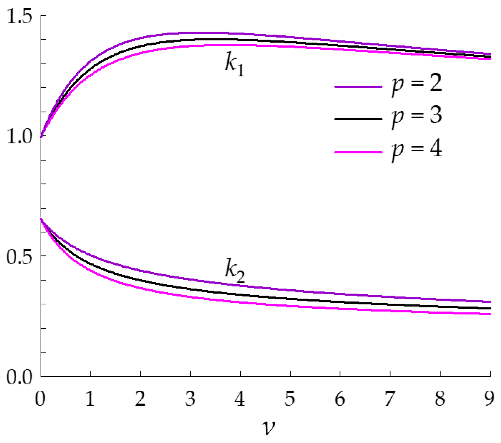
3.1. Dependence of the Model Parameters on $\dot{\epsilon }$, T, and C

Simple strain rate, temperature, and solute concentration dependences are now assigned to the mesoscale model parameters. On the basis of experimental data from Ni-Nb alloys [18] and austenitic stainless steels [19], and for the sake of simplicity, the two exponents p and ν are considered as constants. The hardening parameter H is assumed to depend on strain rate and temperature according to a power law and an inverse Arrhenius equation, respectively, in the same way as a flow stress. In addition, a power law dependence with respect to the solute concentration C is introduced:

$$H=H_0{\dot{\epsilon }}^{m_H}\exp (m_H{Q}_H/RT)C^{n_C},$$

(9)

where mH and QH are the strain rate sensitivity and apparent activation energy of H. According to the literature, the exponent nC is usually close to 0.5 [20].

The grain boundary mobility M (or rather the product Mτ) is assumed in turn to be related to strain rate by a power law equation, and to temperature by a classical Arrhenius exponential [21]. The effect of solutes is introduced according to the Cahn model [22]:

$$M\tau =\frac{(M_0\tau ){\dot{\epsilon }}^{m_M}\exp (-Q_M/RT)}{1+\beta C},$$

(10)

where mM and QM are the strain rate sensitivity and apparent activation energy of Mτ.

Finally, in the absence of experimental data about dynamic nucleation kinetics, kN is tentatively supposed to follow the same model as Mτ and independent of the solute concentration:

$$k_N=k_{N_0}{\dot{\epsilon }}^{m_N}\exp (-Q_N/RT),$$

(11)

where mN and QN are the strain rate sensitivity and apparent activation energy of kN. According to Equations (9)–(11), the present model involves eight constitutive parameters, i.e., mH, QH, mM, QM, mN, QN, nC, and β.

3.2. Effects of Strain Rate, Temperature, and Solute Concentration on Flow Stress and Grain Size

From Equations (5) and (6), it easy to derive the strain rate sensitivity $m=(\partial \ln {\sigma }_s/\partial \ln \dot{\epsilon }{)}_{T,C}$ where the partial derivative with respect to $\dot{\epsilon }$ is calculated with temperature and solute concentration held constant:

$$m=\frac{3(\nu +1)m_H-2m_M-m_N+3}{2(p+3\nu +5)}.$$

(12)

If the exponents mH, mM, and mN are constant as assumed above, m itself is a constant; in particular, it does not depend on the solute fraction C. If we take $p=3$ and $\nu =0$, m becomes:

$$m=\frac{3m_H-2m_M-m_N+3}{16},$$

(13)

and if furthermore the mesoscopic mechanisms, i.e., strain hardening, grain boundary migration, and nucleation, are not rate sensitive, $m_H=m_M=m_N=0$, and $m=3/16\approx 0.188$, a classical value within the hot working range. If by contrast the mesoscopic mechanisms are thermally activated and mH, mM, and mN take the same value, we find again $m=3/16$. In the case where mH, mM, and mN take different but similar values, the sum $3m_H-2m_M-m_N$ acts as a small correction with respect to 3. This shows that DDRX induces a strain rate sensitivity of the flow stress on its own, whatever the strain rate sensitivities of the underlying physical mechanisms.

The apparent activation energy of the flow stress is derived in turn from Equations (5) and (6) using the classical definition $Q=(R/m)[\partial \ln {\sigma }_s/\partial (1/T){]}_{\dot{\epsilon },C}$ where the partial derivative with respect to $1/T$ is calculated with strain rate and solute concentration held constant:

$$Q=\frac{3(\nu +1)m_H{Q}_H+2Q_M+Q_N}{3(\nu +1)m_H-2m_M-m_N+3}.$$

(14)

If mH, QH, mM, QM, mN, QN are constant, Q is a constant as well and it does not depend on the solute content C. Furthermore, assuming that the mesoscopic mechanisms are not thermally activated ($Q_H=Q_M=Q_N=0$) leads to $Q=0$ as well. The overall activation energy Q thus merely reflects the activation energies of the physical mechanisms. If QH, QM, and QN take the same value, for instance Qa, the activation energy for self diffusion, $Q=Q_a$, and if QH, QM, and QN take values close to Qa, Q will also be close to this value, as observed in many instances in practice.

In addition to the usual strain rate and activation energy of the flow stress, it is convenient to define their counterparts for the steady state average grain size, i.e., $m^{\prime }=-(\partial \ln D_s/\partial \ln \dot{\epsilon }{)}_{T,C}$ and $Q^{\prime }=-(R/m^{\prime })[\partial \ln D_s/\partial (1/T){]}_{\dot{\epsilon },C}$, where the minus signs have been introduced for getting positive quantities in the most frequent cases. From Equation (8), it is straightforward to get:

$$m^{\prime }=\frac{(p-1)(\nu +1)m_H-(p+\nu +1)m_M+(\nu +2)m_N+p-1}{p+3\nu +5}.$$

(15)

This equation shows that, in the same way as m, $m^{\prime }$ does not vanish if $m_H=m_M=m_N=0$. For $p=3$ and $\nu =0$, $m^{\prime }=1/4$, to be compared to $m=3/16$ with the same assumptions. Similarly:

$$Q^{\prime }=\frac{(p-1)(\nu +1)m_H{Q}_H+(p+\nu +1)Q_M-(\nu +2)Q_N}{(p-1)(\nu +1)m_H-(p+\nu +1)m_M+(\nu +2)m_N+p-1},$$

(16)

which, like Q, vanishes when $Q_H=Q_M=Q_N=0$.

Finally, it is necessary to introduce two new parameters to assess the effects of the solute content C on steady state flow stress and grain size. In view of Equation (10) where C is not involved in a power law form, single logarithmic derivatives seem to be the most appropriate. We therefore define $\xi =(\partial \ln {\sigma }_s/\partial C{)}_{\dot{\epsilon },T}$, which gives from Equations (5) and (6):

$$\xi =\frac{1}{p+3\nu +5}\left[\frac{3}{2}(\nu +1)\frac{n_C}{C}+\frac{\beta }{1+\beta C}\right],$$

(17)

and similarly ${\xi }^{\prime }=(-\partial \ln D_s/\partial C{)}_{\dot{\epsilon },T}$, which gives from Equation (8):

$${\xi }^{\prime }=\frac{1}{p+3\nu +5}\left[(p-1)(\nu +1)\frac{n_C}{C}+(p+\nu +1)\frac{\beta }{1+\beta C}\right],$$

(18)

where the minus sign has been introduced to get ${\xi }^{\prime }>0$ accounting for the fact that DS decreases with increasing C. In Equations (17) and (18), the first and second terms in the brackets are associated with the influence of C on strain hardening and grain boundary mobility, respectively. Since $p>1$, ${\xi }^{\prime }>\xi$, which implies that, with the above definitions, DS is more sensitive than σS to the solute content. It is also noteworthy that $\xi$ and ${\xi }^{\prime }$ are both decreasing functions of C and tend to infinity when $C\to 0$. This means that the influence of solutes on flow stress and grain size is larger at small concentrations and decreases at larger values of C.

3.3. The Derby Exponents

It has been shown by Derby [23] on the basis of a large number of experimental data pertaining to pure metals and metal alloys, as well as on minerals and ice, that the steady flow stress and average grain size associated with DDRX are related by an inverse power law equation:

$${\sigma }_s=\frac{A}{D_s{}^a},$$

(19)

where A is a constant for a given material and the exponent a falls within the range 0.6–0.8 (Figure 3).

Equation (19) can be written in a symbolic way $a=\delta \ln {\sigma }_s/\delta \ln D_s$. However, this does not represent a true derivative since ${\sigma }_s(\dot{\epsilon },T,C)$ is not a single valued function of $D_s(\dot{\epsilon },T,C)$. It is thus better to use partial derivatives of σS and DS with respect to the external variables $\dot{\epsilon }$, T, and C, which leads automatically to the definition of three distinct Derby exponents, referred to as $a_{\dot{\epsilon }}$, $a_T$, and $a_C$.

(i)

Temperature and solute concentration remain constant (i.e., σS and DS are measured on a single material at given temperature). Only the strain rate varies:

$$a_{\dot{\epsilon }}=-\frac{(\partial \ln {\sigma }_s/\partial \ln \dot{\epsilon }{)}_{T,C}}{(\partial \ln D_s/\partial \ln \dot{\epsilon }{)}_{T,C}},$$

(20)

which is directly related to the strain rate sensitivity exponents by $a_{\dot{\epsilon }}=m/m^{\prime }$. This yields:

$$a_{\dot{\epsilon }}=\frac{1}{2}\frac{3(\nu +1)m_H-2m_M-m_N+3}{(p-1)(\nu +1)m_H-(p+\nu +1)m_M+(\nu +2)m_N+p-1}.$$

(21)

(ii)

Strain rate and solute concentration remain constant (single material at given strain rate). Temperature is the only variable:

$$a_T=-\frac{[\partial \ln {\sigma }_s/\partial \ln {(1/T)]}_{\dot{\epsilon },C}}{[\partial \ln D_s/\partial \ln {(1/T)]}_{\dot{\epsilon },C}},$$

(22)

which can be written in the simple form $a_T=mQ/m^{\prime }{Q}^{\prime }$. This gives:

$$a_T=\frac{1}{2}\frac{3(\nu +1)m_H{Q}_H+2Q_M+Q_N}{(p-1)(\nu +1)m_H{Q}_H+(p+\nu +1)Q_M-(\nu +2)Q_N}.$$

(23)

The two “Derby exponents” $a_{\dot{\epsilon }}$ and $a_T$ are generally distinct. However, if $m_H=m_M=m_N$ and $Q_H=Q_M=Q_N$ (whatever ν and p), they take the same value $a_0=3/[2(p-1)]$. Therefore, if mH, mM, and mN on the one hand, and QH, QM, and QN on the other hand, take different but similar values, $a_{\dot{\epsilon }}$ and $a_T$ are likely to be close to a0. For $p=3$, $a_0=0.75$, which is in good agreement with the observations of Derby. For this reason, $p=3$ was most often chosen until now in the mesoscale model [14,15,19].

Strain rate and temperature remain constant. Solute concentration is the only variable (σS and DS are measured on a series of solid solutions at same strain rate and temperature):

$$a_C=-\frac{[\partial \ln {\sigma }_s/\partial C{]}_{\dot{\epsilon },T}}{[\partial \ln D_s/\partial C{]}_{\dot{\epsilon },T}},$$

(24)

which can also be written in the form $a_C=\xi /{\xi }^{\prime }$. Thus:

$$a_C=\frac{\frac{3}{2}(\nu +1)n_C+\frac{\beta C}{1+\beta C}}{(p-1)(\nu +1)n_C+(p+\nu +1)\frac{\beta C}{1+\beta C}}.$$

(25)

It is important to note that, unlike $a_{\dot{\epsilon }}$ and $a_T$, this third “Derby exponent” does not depend on the strain rate sensitivities and activation energies, but it is a function of C.

Figure 4 shows such dependence for $n_C=0.5$, $\beta =4\times {10}^4$ (after [24]), and various values of ν and p. For $C=0$ (pure metal), $a_C=a_0$, which is consistent with the above results. With increasing solute content, aC decreases rapidly to reach a constant value for $C\approx {10}^{-3}$ (i.e., 0.1%). The latter depends only on ν and p. For instance, with $\nu =0$ and $p=3$, Equation (25) gives $a_C=0.35$, a value significantly less than a0.

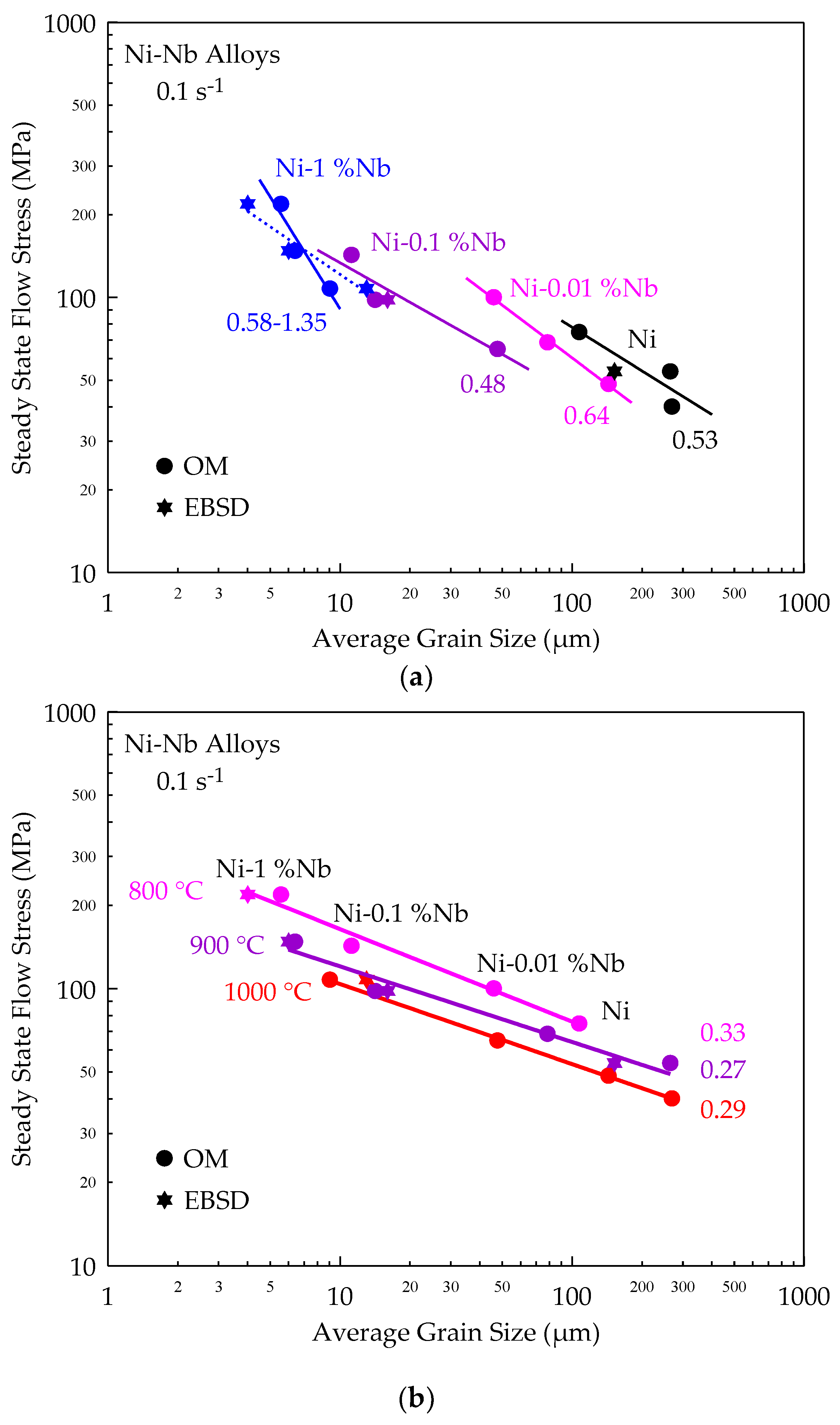
3.4. Application to a Set of Ni-Nb Alloys

The above results are now illustrated with experimental data pertaining to a series of high purity base Ni-Nb alloys including high purity nickel, Ni-0.01%Nb, Ni-0.1%Nb, and Ni-1%Nb. They were obtained from hot torsion tests carried out at 800, 900, and 1000 °C and 0.1 s⁻¹ up to the steady state flow stress ($\epsilon =5$) [18]. The average grain sizes were measured by optical microscopy (OM) and in some cases by Electron Backscattering Diffraction (EBSD) in order to plot a $\ln D_s-\ln {\sigma }_s$ “Derby diagram”. In Figure 5a, linear fits are drawn for each alloy (i.e., only the temperature varies) to determine the exponent aT. Values of 0.53, 0.64, 0.48 are obtained for pure nickel, Ni-0.01%Nb, and Ni-0.1%Nb, respectively; an uncertain value ranging from 0.58 to 1.35 is estimated for the Ni-1%Nb alloy. All these aT exponents fall within the lower range of the classical “Derby exponents”. On the other hand, in Figure 5b, linear fits are drawn for each temperature (i.e., only the solute concentration changes) to determine the exponent aC. Values of 0.33, 0.27, and 0.29 are observed at 800, 900, and 1000 °C, respectively. The latter are significantly less than the former aT values. This is in agreement with the above model which predicts aC values ranging from 0.3 to 0.4 for solute contents larger than 10⁻⁴ (0.01%), while $a_T=a_0=0.75$ (assuming p = 3), although this value is an overestimation in the present case.

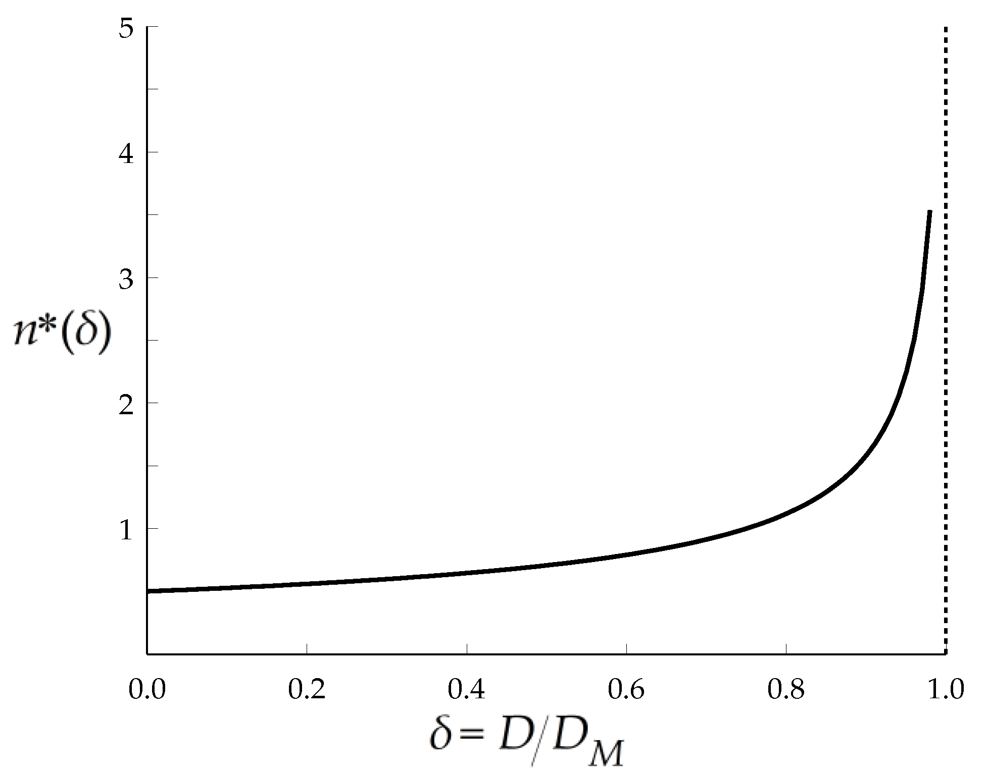
4. Steady State Grain Size Distribution

Until now, only average quantities such as the steady state grain size Ds and dislocation density ρs were considered. It is shown in this section that, to some extent, distributions of the macroscopic parameters of interest can be derived from the mesoscopic model as well. The following development focuses on grain size distributions, but it could be applied in the same way to any other quantity.

4.1. Model Involving a Single Family of Grains

The grain size distribution function $n(D)$ is defined such that $n(D)\mathrm{d}D$ is the number fraction of grains of size (diameter) ranging between D and $D+\mathrm{d}D$ among a set of N grains (surface or volume fractions can be used as well). Consider first a set of grains with identical parameters M, H, ν, kN, and p. The size history $D(t)$ is also the same for each grain. Furthermore, when a steady state is established, the nucleation rate does not depend on time, so that the number of grains of age t does not depend on t ($0\le t\le t_{end}$). Using the ergodic assumption, this means that $n(D)\mathrm{d}D$ is equal to the ratio $(\mathrm{d}{t}_G+\mathrm{d}{t}_S)/t_{end}$, where $\mathrm{d}{t}_G$ is the time during which the size of a growing grain ranges between D and $D+\mathrm{d}D$, while $\mathrm{d}{t}_S$ is the time during which the size of a shrinking grain ranges between $D+\mathrm{d}D$ and D, as illustrated in the diagram of Figure 6. (Growing and shrinking grains will not be distinguished here.) Since $\mathrm{d}t=\mathrm{d}D/(\mathrm{d}D/\mathrm{d}t)$, this can be written in the form:

$$n(D)=\frac{1}{t_{end}}\left[\frac{1}{(\mathrm{d}D/\mathrm{d}t{)}_G}-\frac{1}{(\mathrm{d}D/\mathrm{d}t{)}_S}\right].$$

(26)

In the simple case where $\nu =0$, a combination of Equations (1) and (2) leads to:

$$\frac{\mathrm{d}D}{\mathrm{d}t}=2M\tau (\overline{\rho }-H\dot{\epsilon }t),$$

(27a)

$$D=2M\tau t(\overline{\rho }-H\dot{\epsilon }t/2),$$

(27b)

(with $D_0=0$). The curve $D(t)$ is merely a parabola, the maximum size $D_M=M\tau {\overline{\rho }}^2/H\dot{\epsilon }$ occurring for $t_M=\overline{\rho }/H\dot{\epsilon }$, and the lifetime of every grain is $t_{end}=2t_M=2\overline{\rho }/H\dot{\epsilon }$. Equation (26) then reduces to:

$$n(D)=\frac{2}{t_{end}}\frac{1}{(\mathrm{d}D/\mathrm{d}t{)}_G}.$$

(28)

Solving Equation (27b) for t gives for $t\le t_M$:

$$t=\frac{\overline{\rho }}{H\dot{\epsilon }}\left(1-\sqrt{1-\frac{D}{D_M}}\right).$$

(29)

Substituting this expression into Equations (27a) and (28) leads after simplification to:

$$n(D)=\frac{1}{2\sqrt{D_M(D_M-D)}}.$$

(30)

(The integral of $n(D)$ from $D=0$ to $D_M$ is of course equal to unity). It is convenient to introduce the normalized grain size $\delta =D/D_M$ and then it is easy to check that the distribution function of this new variable is $n^{*}(\delta )=D_{M}n(D)$, i.e.,:

$$n^{*}(\delta )=\frac{1}{2\sqrt{1-\delta }}.$$

(31)

This function is monotonically increasing and tends to infinity when δ approaches 1 (Figure 7). It is definitely a very unrealistic prediction of the real steady state DDRX grain size distributions, which are known to be approximately log-normal. The origin of this failure appears clearly in Equation (28), which shows that $n(D)$ becomes infinite when $\mathrm{d}D/\mathrm{d}t=0$, i.e., when $D=D_M$. Since only one family of grains is considered, there are infinitely many grains of size close to DM in the aggregate.

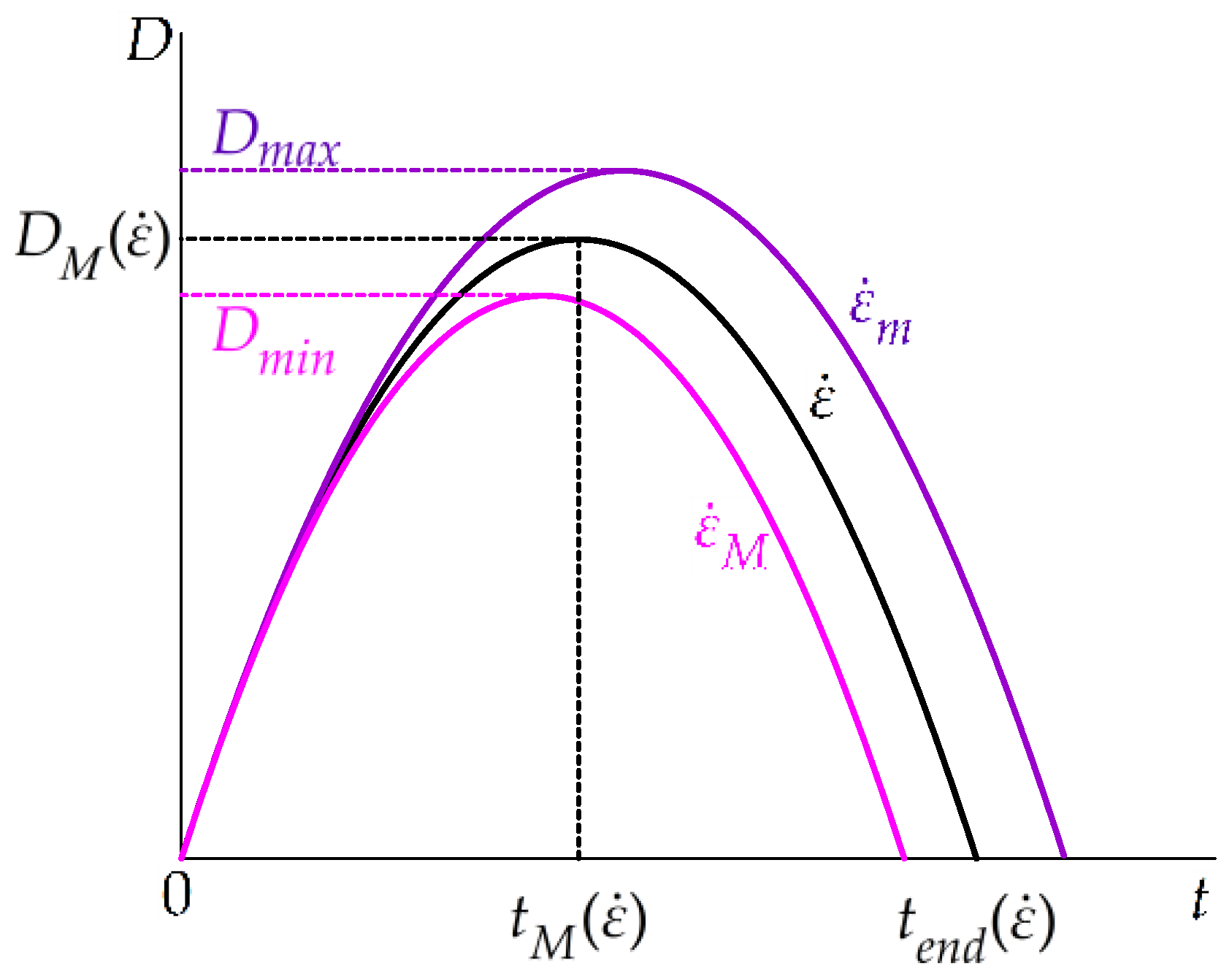
4.2. Models Involving Several Family of Grains

There have been various attempts to solve the above problem. The analytic expression of the maximum grain size for one family of grains, viz. $D_M=M\tau {\overline{\rho }}^2/H\dot{\epsilon }$, shows that it increases with the grain boundary mobility M. In an aggregate of grains, M needs not be constant because it depends of the crystalline orientations of the grains on both sides of the boundary. The effects of introducing a distribution of M on the steady state grain size distributions have been therefore investigated, leading to quite encouraging results [25]. Similarly, DM is a decreasing function of the strain hardening parameter H and the effect of a distribution of H, associated with the various orientations of the grains has been briefly addressed in [26]. It can be argued as well that grains deform at different strain rates according to their Taylor factor MT, largest values of MT corresponding to lowest $\dot{\epsilon }$ and conversely. The strain rate of a grain is also known to be influenced by the orientation of its neighbours. In the present case where simple power law strain hardening is considered, Equation (27b) shows that $\dot{\epsilon }$ and H play the same role in the model (which would not be true for other strain hardening laws, e.g., the Kocks–Mecking or Yoshie–Laasraoui–Jonas equations).

Hereafter, in this paper, an infinite number of grain families is considered (each family includes itself infinitely many grains), each of them being submitted to a specific strain rate $\dot{\epsilon }$. A distribution function $\phi (\dot{\epsilon })$ is therefore introduced, meaning that $\phi (\dot{\epsilon })\mathrm{d}\dot{\epsilon }$ is the number fraction of grains that undergo a strain rate ranging between $\dot{\epsilon }$ and $\dot{\epsilon }+\mathrm{d}\dot{\epsilon }$, with the normalization condition:

$${\displaystyle {\int }_{{\dot{\epsilon }}_m}^{{\dot{\epsilon }}_M}\phi (\dot{\epsilon })\mathrm{d}\dot{\epsilon }=1},$$

(32)

where ${\dot{\epsilon }}_m$ and ${\dot{\epsilon }}_M$ denote the minimum and maximum strain rates in the aggregate. For each family, Equation (27a,b) still holds, which means that (with $\nu =0$) the grain size history $D(t)$ is described by a parabola with maximum $D_M(\dot{\epsilon })=M\tau {\overline{\rho }}^2/H\dot{\epsilon }$ and lifetime $t_{end}(\dot{\epsilon })=2\overline{\rho }/H\dot{\epsilon }$ (Figure 8). Note that the minimum strain rate ${\dot{\epsilon }}_m$ is associated with the largest maximum size $D_M({\dot{\epsilon }}_m)=D_{max}$ and the largest lifetime $t_{end}({\dot{\epsilon }}_m)$; conversely, the maximum strain rate corresponds to the lowest maximum grain size $D_M({\dot{\epsilon }}_M)=D_{min}$. Furthermore, $D_M(\dot{\epsilon })/D_{max}={\dot{\epsilon }}_m/\dot{\epsilon }$. The distribution is given by Equation (30) where D_M is replaced by its expression given above depending on $\dot{\epsilon }$:

$$n(D,\dot{\epsilon })=\frac{1}{2{\dot{\epsilon }}_m{D}_{\max }}\frac{\dot{\epsilon }}{\sqrt{1-\delta \frac{\dot{\epsilon }}{{\dot{\epsilon }}_m}}},$$

(33)

where δ is the normalized grain size $D/D_{max}$. For obtaining the distribution function $n(D)$, $n(D,\dot{\epsilon })$ must now be weighted by $\phi (\dot{\epsilon })$ and integrated with respect to $\dot{\epsilon }$. Two cases are to be considered (Figure 8):

-

When $0\le D\le D_{min}$, or $0\le \delta \le r$, where $r=D_{min}/D_{max}={\dot{\epsilon }}_m/{\dot{\epsilon }}_M$, all grain families contribute to the distribution. The integration is thus extended over the whole interval $[{\dot{\epsilon }}_m,{\dot{\epsilon }}_M]$.

-

When $D_{min}\le D\le D_{max}$, or $r\le \delta \le 1$, only the grains such that $D_M(\dot{\epsilon })>D$, i.e., grains undergoing a strain rate $\dot{\epsilon }<M\tau {\overline{\rho }}^2/HD$ or $\dot{\epsilon }<{\dot{\epsilon }}_m{D}_{max}/D$ contribute to the distribution. The interval of integration is now $[{\dot{\epsilon }}_m,{\dot{\epsilon }}_m{D}_{max}/D]$ or $[{\dot{\epsilon }}_m,{\dot{\epsilon }}_m/\delta ]$.

For the sake of simplicity, a constant distribution of the strain rate is chosen here, i.e., $\phi (\dot{\epsilon })=1/({\dot{\epsilon }}_M-{\dot{\epsilon }}_m)$ to meet the normalization requirement (Equation (32)).

After calculation, this gives the distribution function of the normalized grain size $n^{*}(\delta )=D_{max}n(D)$:

-

For $0\le \delta \le r$:

$$n^{*}(\delta )=\frac{r}{1-r}\frac{1}{{\delta }^2}\left[\frac{1}{3}{\left(1-\frac{\delta }{r}\right)}^{3/2}-\frac{1}{3}{(1-\delta )}^{3/2}-{\left(1-\frac{\delta }{r}\right)}^{1/2}+{(1-\delta )}^{1/2}\right],$$

(34a)

-

for $r\le \delta \le 1$:

$$n^{*}(\delta )=\frac{r}{1-r}\frac{1}{{\delta }^2}\left[{(1-\delta )}^{1/2}-\frac{1}{3}{(1-\delta )}^{3/2}\right].$$

(34b)

Three distributions are displayed in Figure 9a for $r={\dot{\epsilon }}_{min}/{\dot{\epsilon }}_{max}$ = 0.2, 0.4, and 0.6. Evaluation of the indeterminate form of Equation (34a) when $\delta \to 0$ gives $n^{*}(0)=(1+r)/4r$. The maximum value is obtained from both Equation (34a,b) for $\delta =r$; furthermore, $n^{*}(1)=0$. An experimental DDRX steady state grain size distribution pertaining to A304 stainless steel strained in torsion at 1050 °C is reported in Figure 9b [27]. It is in rather good agreement with the theoretical distribution for r = 0.2 in Figure 9a. There is, however, a significant discrepancy for values of δ less than approximately 0.1. This is likely to result from the fact that the experimental distribution was built from EBSD two-dimensional measurements of the grain sizes. This technique is known to underestimate the number of small grains because the probability to intersect the latter is low. In contrast, the model is intrinsically three-dimensional and thus predicts the true distribution, which results in larger $n^{*}(\delta )$ values for small grain sizes.

It is worth noting that the agreement obtained for r = 0.2 does not mean that such a large spread of strain rates really occurs in the material, but the above calculations suggest that the experimental distributions can be well explained by the scattering of material parameters, e.g., H or M, and local strain rates $\dot{\epsilon }$. Other comparisons with experimental steady state grain size distributions should be carried out in the future. It is nevertheless already well established that they display a log-normal shape as predicted by the model [28].

5. Conclusions

In this paper, an analytical grain scale (mesoscopic) DDRX model was first briefly presented, in a simplified version where strain hardening is described by a power law function. Closed form equations have been obtained for the steady state. While this approach has so far been limited to the overall behaviour of pure metals, and only average values of DRX grain sizes have been considered, three original extensions were developed in the present paper. The model allows:

(1)

To derive the macroscopic constitutive parameters m and Q associated with DDRX as functions of the mesoscopic parameters of the model, for pure metals and solid solutions.

(2)

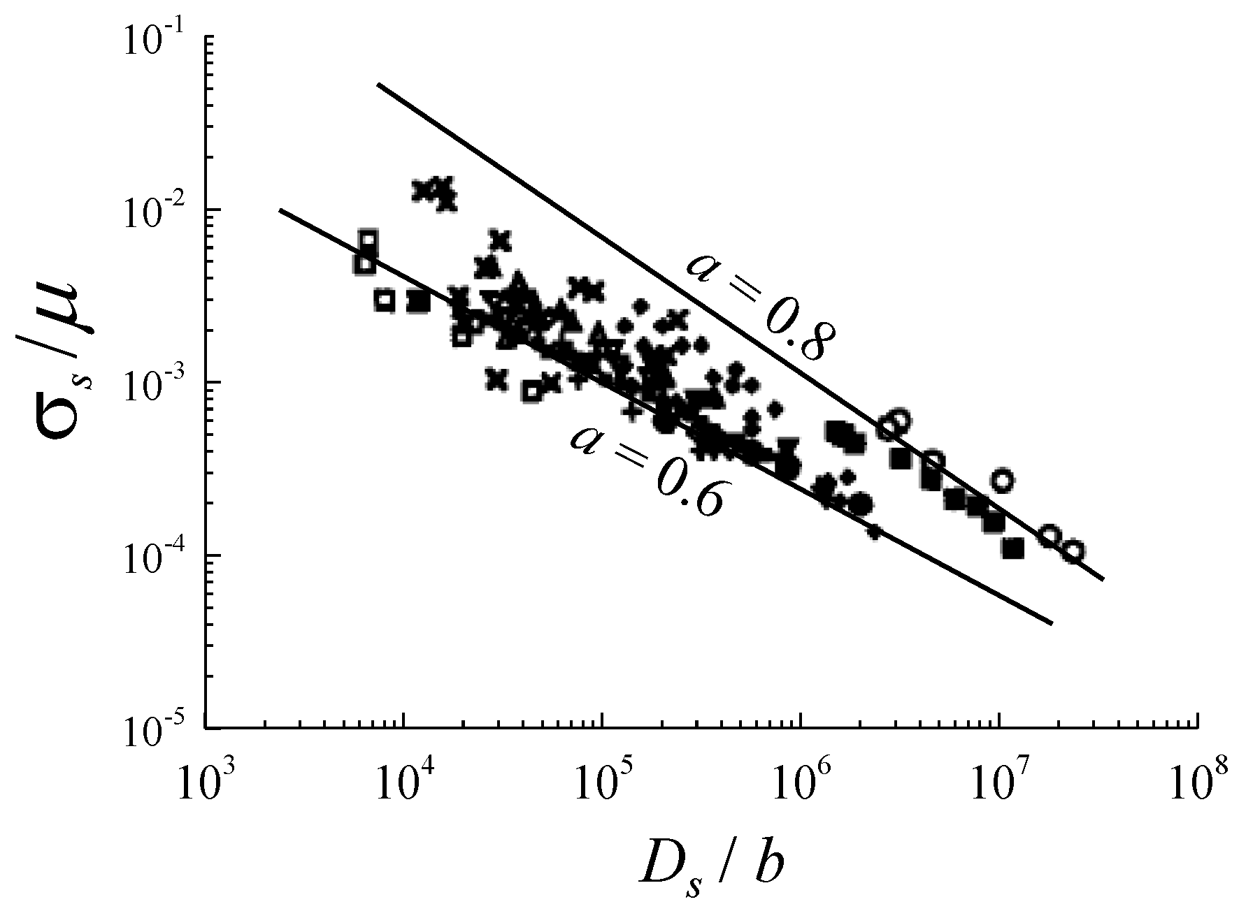
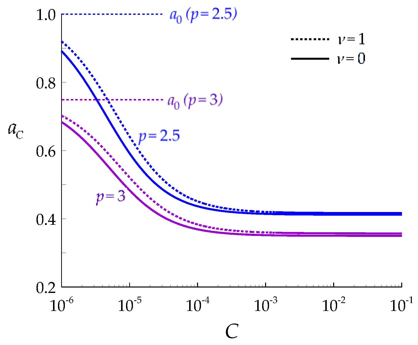
To show that the inverse power law relationship (“Derby equation”) between the steady state flow stress and average grain size is verified. Moreover, the analysis leads to define three, instead of one, “Derby exponents” $a_{\dot{\epsilon }}$, aT, and aC, according to whether the strain rate $\dot{\epsilon }$, the temperature T, or the solute content C is the only variable of the system. An important result is that aC is less than the two other exponents, a prediction that is well verified in the case of a set of Ni-Nb alloys.

(3)

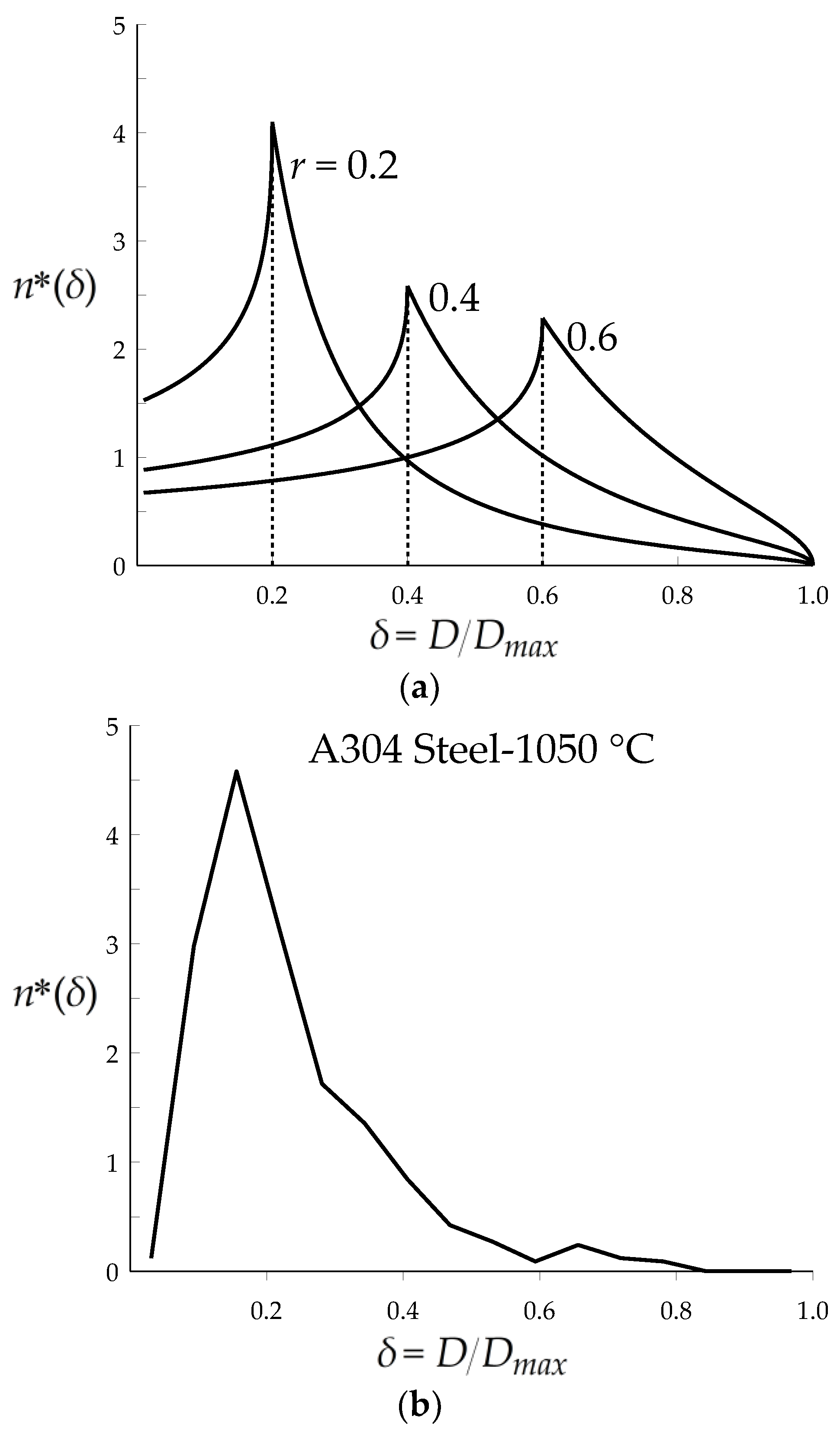
In addition, the mesoscale model allows for predicting not only average values of parameters such as the grain size or the dislocation density, but also their distributions, if the mesoscale parameters or the strain rate of the grains are scattered. This was illustrated by introducing a uniform strain rate distribution over the grains of the aggregate.

Finally, it is suggested that, even in our time, analytical approaches are still able to provide valuable information about the physical phenomena associated with DDRX (as well as in other circumstances), and to lead to a better understanding of the relations between meso and macroscopic scales. Therefore, they still have their place besides, and as far as possible interacting with, numerical simulations.

References

1. Stüwe, H.P.; Ortner, B. Recrystallization in hot working and creep. Met. Sci. 1974, 8, 161–167. [Google Scholar] [CrossRef]
2. Sandström, R.; Lagneborg, R. A model for hot working occurring by recrystallization. Acta Metall. 1975, 23, 387–398. [Google Scholar] [CrossRef]
3. Rollett, A.D.; Luton, M.J.; Srolovitz, D.J. Microstructural simulation of dynamic recrystallization. Acta Metall. Mater. 1992, 40, 43–55. [Google Scholar] [CrossRef]
4. Luton, M.J.; Peczak, P. Monte Carlo modeling of dynamic recrystallization: Recent developments. Mater. Sci. Forum 1993, 113–115, 67–80. [Google Scholar] [CrossRef]
5. Peczak, P. A Monte Carlo study of influence of deformation temperature on dynamic recrystallization. Acta Metall. Mater. 1995, 43, 1279–1291. [Google Scholar] [CrossRef]
6. Goetz, R.L.; Seetharaman, V. Modeling dynamic recrystallization using cellular automata. Scr. Mater. 1984, 38, 405–413. [Google Scholar] [CrossRef]
7. De Jaeger, J.; Solas, D.; Fandeur, O.; Schmitt, J.-H.; Rey, C. 3D numerical modeling of dynamic recrystallization under hot working: Application to Inconel 718. Mater. Sci. Eng. A 2015, 646, 33–44. [Google Scholar] [CrossRef]
8. Cui, Z.; Jin, Z. Investigation on strain dependence of dynamic recrystallization behavior using an inverse analysis method. Mater. Sci. Eng. A 2010, 527, 3111–3119. [Google Scholar]
9. Bernacki, M.; Resk, H.; Coupez, T.; Logé, R. Finite element model of primary recrystallization in polycrystalline aggregates using a level set framework. Model. Simul. Mater. Sci. Eng. 2009, 17, 1–22. [Google Scholar] [CrossRef] [Green Version]
10. Maire, L.; Scholtes, B.; Moussa, C.; Bozzolo, N.; Pino Muñoz, D.; Settefrati, A.; Bernacki, M. Modeling of dynamic and post-dynamic recrystallization by coupling a full field approach to phenomenological laws. Mater. Des. 2017, 133, 498–519. [Google Scholar] [CrossRef] [Green Version]
11. Lieou, C.K.C.; Bronkhorst, C.A. Dynamic recrystallization in adiabatic shear banding: Effective-temperature model and comparison to experiments in ultrafine-grained titanium. Int. J. Plast. 2018, in press. [Google Scholar] [CrossRef]
12. Lieou, C.K.C.; Mourad, H.M.; Bronkhorst, C.A. Strain localization and dynamic recrystallization in polycrystalline metals: Thermodynamic theory and simulation framework. arXiv, 2018; arXiv:1808.07454. [Google Scholar]
13. Huang, K.; Logé, R. A review on dynamic recrystallization phenomena in metallic materials. Mater. Des. 2016, 111, 548–574. [Google Scholar] [CrossRef]
14. Montheillet, F.; Lurdos, O.; Damamme, G. A grain scale approach for modeling steady state discontinuous dynamic recrystallization. Acta Mater. 2009, 57, 1602–1612. [Google Scholar] [CrossRef]
15. Montheillet, F.; Jonas, J.J. Models of recrystallization. In Fundamentals of Modeling for Metals Processing, ASM Handbook; Furrer, D.U., Semiatin, S.L., Eds.; ASM International: Materials Park, OH, USA, 2009; Volume 22A, pp. 220–231. [Google Scholar]
16. Estrin, Y.; Mecking, H. A unified phenomenological description of work hardening and creep based on one-parameter models. Acta Metall. 1984, 32, 57–70. [Google Scholar] [CrossRef]
17. Laasraoui, A.; Jonas, J.J. Prediction of steel flow stresses at high temperatures and strain rates. Metall. Trans. A 1991, 22, 1545–1558. [Google Scholar] [CrossRef]
18. Maatougui, N.; Piot, D.; Fares, L.; Montheillet, F.; Semiatin, S.L. Influence of niobium solutes on the mechanical behaviour of nickel during hot working. Mater. Sci. Eng. A 2013, 586, 350–357. [Google Scholar] [CrossRef]
19. Piot, D.; Smagghe, G.; Jonas, J.J.; Desrayaud, C.; Montheillet, F.; Perrin, G.; Montouchet, A.; Kermouche, G. A semitopological mean-field model of discontinuous dynamic recrystallization. J. Mater. Sci. 2018, 53, 8554–8566. [Google Scholar]
20. Estrin, Y. Dislocation-density-related constitutive modeling. In Unified Constitutive Laws of Plastic Deformation; Krausz, A.S., Krausz, K., Eds.; Elsevier: Amsterdam, The Netherlands, 1996; Chapter 2. [Google Scholar]
21. Humphreys, F.J.; Hatherly, M. Recrystallization and Related Annealing Phenomena, 2nd ed.; Elsevier: Amsterdam, The Netherlands, 2008; p. 123. [Google Scholar]
22. Cahn, J.W. The impurity-drag effect in grain boundary motion. Acta Metall. 1962, 10, 789–798. [Google Scholar] [CrossRef]
23. Derby, B. Dynamic recrystallization: The steady state grain size. Scr. Metall. Mater. 1992, 27, 1581–1585. [Google Scholar] [CrossRef]
24. Piot, D.; Smagghe, G.; Montheillet, F. Modeling grain-boundary mobility and nucleation rate during discontinuous dynamic recrystallization in Ni-Nb alloys and a high-purity alloy derived from SAE 304L. Mater. Sci. Forum 2017, 879, 1501–1506. [Google Scholar] [CrossRef]
25. Piot, D.; Damamme, G.; Montheillet, F. Mesoscopic modeling of discontinuous dynamic recrystallization: Steady state grain size distributions. Mater. Sci. Forum 2012, 706–709, 234–239. [Google Scholar] [CrossRef]
26. Montheillet, F.; Thomas, J.-P.; Damamme, G. Distribution de la taille des grains recristallisés dynamiquement dans les matériaux métalliques. In Proceedings of the Congrès Matériaux 2002 CD-ROM, Tours, France, 21–25 October 2002. [Google Scholar]
27. Smagghe, G. Modélisation de la Recristallisation lors du Forgeage à Chaud de l’acier 304L—Une Approche Semi-Topologique pour les Modèles en Champ Moyen. Ph.D. Thesis, Ecole des Mines de Saint-Etienne, Saint-Étienne, France, 2017. [Google Scholar]
28. Favre, J. Recrystallization of L-605 Cobalt Superalloy during Hot Working Process. Ph.D. Thesis, Tohoku University, Sendai, Japan, INSA, Lyon, France, 2012. [Google Scholar]
Figure 1. Schematic representation of a grain in the aggregate: (a) grain growth ( ρ < ρ ¯ ); (b) grain shrinkage ( ρ > ρ ¯ ).
Metals 08 00789 g001
Figure 2. Dependence of the factors k1 and k2 of Equations (5) and (8) on the strain hardening exponent ν for three values of the nucleation exponent p.
Metals 08 00789 g002
Figure 3. Double logarithmic “Derby diagram” highlighting the experimental relationship between the steady state flow stress and grain size associated with DRX. Note that materials undergoing CDRX (continuous dynamic recrystallization), e.g., NaCl and olivine, as well as DDRX are included in the data. The flow stress and grain size are normalized by the elastic shear modulus µ and Burgers vector b, respectively. The majority of the points fall between the two straight lines of slopes 0.6 and 0.8 (after [23]).
Metals 08 00789 g003
Figure 4. Dependence of the third “Derby parameter” aC on the solute concentration C for ν = 0 and 1, and p = 2.5 and 3 with nC = 0.5 and β = 4 × 10 4 . The values (a0) taken by aC for C = 0 are indicated by broken lines.
Metals 08 00789 g004
Figure 5. ln D s ln σ s “Derby plots” pertaining to four high purity base Ni-Nb alloys, i.e., pure nickel, Ni-0.01%Nb, Ni-0.1%Nb, and Ni-1%Nb strained in torsion up to the steady state at three temperatures: (a) determination of the exponent aT (only the temperature varies); (b) determination of the exponent aC (only the solute content varies). Numerical values of the exponents are indicated.
Metals 08 00789 g005
Figure 6. Diagram showing a grain size evolution along its lifetime. The number fraction of grains of size (diameter) ranging between D and D + d D is equal to ( d t G + d t S ) / t e n d .
Metals 08 00789 g006
Figure 7. Normalized steady state DDRX grain size distribution when a single family of grains is considered.
Metals 08 00789 g007
Figure 8. Grain size histories of three grains nucleated at the same time t = 0 belonging to three different families. The maximum sizes Dmin and Dmax are associated with the maximum ( ε ˙ M ) and minimum ( ε ˙ m ) strain rates, respectively. This diagram shows that all families of grains contribute to the grain size distribution for 0 D D m i n . By contrast, for D m i n D D m a x , only the grains such as D M ( ε ˙ ) > D contribute.
Metals 08 00789 g008
Figure 9. Steady state DDRX grain size distributions: (a) theoretically predicted by the model for a uniform scattering of strain rates with various values of r = ε ˙ m / ε ˙ M ; (b) experimentally measured by EBSD on a A304 stainless steel (after [27]).
Metals 08 00789 g009