Machine Learning-Based Ultimate Strength Prediction of Spherical Shells Considering Multi-Source Uncertain Imperfections

Abstract

Spherical shells are a commonly used structural form in submarine pressure-resistant structures. This study employed machine learning to predict the ultimate strength statistical properties of spherical shells considering inevitable multi-source uncertain imperfections. Thirty nominally identical spherical shells were fabricated, the thickness distribution and geometric imperfections were measured, and the ultimate strength of these shells were obtained by hydrostatic experiments. Then, the measured imperfections were reconstructed and mapped into the finite element model, and the buckling performance of the spherical shells were numerically investigated. Subsequently, two XGBoost models with considerable accuracy were trained to predict the ultimate strength statistical properties. The pole-smoothing double Fourier series expansion was adopted to reconstruct the geometric imperfections with accuracies exceeding 0.985 on all tested shells. The experimental ultimate strength of the spherical shells was consistent with the numerical predictions with an error of 0.81%. The evaluation metrics R² of the XGBoost models for the mean and standard deviation of spherical shell ultimate strength were 0.9977 and 0.9246, respectively. At a confidence level of 99.74%, the margin of the upper bound prediction was 0.018 MPa, and the margin of the lower bound prediction was 0.624 MPa. The findings of this study propose an innovative method to predict the ultimate strength bounds of spherical shells, offering a generalizable workflow that can potentially inform the design of submarine pressure hulls when extended to application-specific geometric dimensions and materials.

1. Introduction

Spherical shells have served as primary load-bearing structures in marine engineering, such as in unmanned underwater vehicles (UUVs) and various deep-sea submersibles [1,2,3]. The ultimate strength of spherical shells subjected to external pressure is a key indicator for evaluating the performance of such structures. However, manufacturing-induced imperfections from various sources are inevitable, severely degrading the ultimate strength of spherical shells. Furthermore, the inherent stochasticity of these imperfections inevitably leads to significant scatter in the ultimate strength [4,5]. Therefore, accurately predicting the ultimate strength of spherical shells with multi-source uncertain imperfections is of great significance for structural design and in-service condition monitoring.

The ultimate strength of spherical shells can be predicted via analytical and numerical methods. Zoelly [6] pioneered the classical formula for predicting elastic buckling loads, which is widely regarded as the cornerstone of shell buckling theory. BiJlaard [7] assumed that plastic deformation is governed by the elastic shearing energy, and derived the differential equations for plate and shell buckling. Nevertheless, imperfections such as manufacturing-induced geometric deviations and thickness variations are inevitable in actual spherical shells. These deviations can severely compromise structural buckling performance, frequently leading to catastrophic buckling failure at loads significantly below theoretical predictions. Therefore, employing appropriate methodologies to account for these imperfections and quantify their influence on load-bearing capacity is of paramount importance. A widely adopted standard is NASA SP-8032, which is frequently employed to evaluate imperfection sensitivity and estimate the lower bound of ultimate strength [8]. Hutchinson [9] expanded the applicability of Koiter’s theory [10] by examining the influence of axisymmetric imperfections on the post-buckling behavior of spherical shells. Evkin et al. [11] investigated the post-buckling regime of imperfect spherical shells subject to small and large deflections through two asymptotic case studies. By combining the respective asymptotic formulations, they derived a formula to predict buckling loads across the entire range of deflection amplitudes. Pan et al. [12] performed a series of nonlinear buckling analyses to evaluate how structural parameters and imperfections affect ultimate strength, subsequently proposing an empirical formula for titanium alloy spherical shells. Wagner et al. [13,14] explored the influence of structural parameters on buckling behavior and developed robust knockdown factors, thereby providing a reliable design methodology for spherical shells. Zhao et al. [15] presented a comprehensive study comparing analytical approaches against experimental data of externally pressurized spherical shells with realistic imperfections and varying geometric parameters. Their findings indicated that current theoretical approaches are still difficult to reconcile with the behavior of actual hulls. Since existing predictive methods are typically derived from idealized theoretical assumptions or extensive finite element (FE) analysis databases, their practical applicability must be further verified and extended.

FE analysis serves as an alternative approach to study the ultimate load of spherical shells, with equivalent defects embedded in simulation models. Zhang et al. [16] evaluated the nonlinear buckling behavior of spherical shells by incorporating eigenmode geometric imperfections, subsequently deriving a semi-analytical formula for ultimate strength prediction based on their numerical results. Wu et al. [17] investigated the quasi-static collapse of spherical pressure hulls by incorporating the first-order buckling mode into their FE model. The resulting simulated collapse loads and modes showed excellent agreement with the experimental findings. Ismail et al. [4] presented a comparative study by introducing eigenmode and single load indentation imperfections into the perfect spherical shell model and proposed a lower-bound closed-form empirical formula for externally pressurized spherical shells. Although introducing assumed modal imperfections to FE models can narrow the gap between the predicted and experimental ultimate strength of spherical shells to some extent, the diverse range of actual imperfections remains unaccounted for. More importantly, the simplified or empirical treatments of imperfections involves substantial subjectivity and arbitrariness. Zhang et al. [18,19] substituted the idealized perfect model with experimentally scanned shell geometries, incorporating measured weld seam thicknesses to investigate the buckling behavior of spherical shells under shape imperfections and through-thickness defects. Although this approach can enhance simulation accuracy, it is difficult to apply to parametric investigations, thereby hindering the revelation of underlying mechanical laws and the development of targeted design methodologies. By coupling welding simulation with nonlinear buckling analysis, Yu et al. [20] developed a predictive model for buckling behavior, the accuracy of which was verified against spherical shells with diverse thickness-to-radius ratios. Abbasi et al. [21] investigated the mechanical response of spherical shells containing a single dimple-like defect to a point probe at different pressurization levels, and concluded that the critical buckling point can only be inferred by tracking the maxima of the indentation force–displacement curves while the probe is implemented sufficiently close to the defect. Ubamanyu et al. [22] conducted a study on the buckling strength of near-perfect spherical shells with small amplitude defects and emphasized the importance of choosing appropriate discretization and solver parameters for buckling mode prediction across different shell geometries. Li et al. [23] established a database from parametric studies on actual submarine spherical shells with various collision loading scenarios, and then summarized empirical equations to predict the residual ultimate strength. Wagner et al. [24] investigated the imperfection sensitivity of spherical domes using the reduced stiffness method, and subsequently proposed an innovative design concept for spherical shells under external pressure. However, most existing studies performed parametric analysis by idealizing imperfection shapes into the spherical shell models, yet such simplifying assumptions are conditional and far from realistic.

Integrating parametric actual imperfections into FE models offers an effective avenue to enhance prediction accuracy and extend the applicability of numerical simulations. In structural engineering, extensively researched cylindrical shells have significantly benefited from the development of diverse, mature techniques for imperfection characterization [25,26,27]. Fina and Bisagni [28] investigated the buckling performance optimization of cylindrical shells by modeling the geometric imperfections as a Fourier series field. Feng et al. [29] characterized arbitrary circumferential thickness variations by combining the perturbation method with Fourier series expansion, thereby quantifying the influence of these variations on the buckling behavior of shells. Wang et al. [30] isolated the geometric imperfections from other defect types using the Fourier series method, revealing the influence of imperfection components and amplitudes on the buckling behavior of quasi-perfect cylindrical shells. Based on the Fourier series method, most references above-mentioned conducted further uncertainty analysis to quantify the mechanism through which random imperfections affect the mechanical properties of cylindrical shells. Compared with case analyses of single deterministic defects, this approach better aligns with the actual service conditions of shells, yielding conclusions with higher reliability and greater practical engineering relevance [31,32]. In the context of spherical shells, Xiong et al. [33] investigated the random characteristics of their ultimate strength by incorporating eigenmodes into FE models, identifying the most critical eigenmode and calculating the corresponding ultimate strength. Zhan et al. [34] categorized the geometric parameters and material properties of spherical shells as distinct types of uncertain variables, and subsequently investigated their effects on the structural ultimate strength. By treating structural parameters and material properties as uncertain inputs, Zulkifli et al. [35] elucidated their influence on the ultimate strength, mode shapes, and stress distributions of spherical shells. However, mathematically formulating the geometric imperfections of spherical shells and mapping them onto FE models to account for their inherent stochasticity can significantly enhance the accuracy and reliability of model-based buckling predictions and subsequent engineering decisions.

Machine learning (ML) provides a powerful framework for predicting the mechanical performance of shells with different structural forms. For example, Ehsani and Dalir [36] optimized the critical buckling load and structural weight of an angle grinder plate using genetic algorithm based on an artificial neural network. Majumder et al. [37] proposed a novel hybrid ML framework integrating Gaussian process regression with extreme gradient boosting for the ultimate strength prediction of conical shells. Wang et al. [38,39] compared the performance of some commonly used models and investigated the failure pressure as well as failure mode of composite cylindrical shells. Their research quantified the relationship between shell failure behavior and structural and material parameters, and provided design recommendations for composite cylindrical shells. Doshi and Ning [40] used extreme gradient boosting to replace the time-consuming FE model to predict the buckling loads of composite near-spherical shells. Given the demonstrated efficacy of ML-based models in capturing the complex mechanical behavior of shells, extending their application to predict the ultimate strength of imperfect spherical shells is highly viable. Nevertheless, to characterize the randomly distributed geometric imperfections with high fidelity, integrating ML models within statistical frameworks remains to be thoroughly explored.

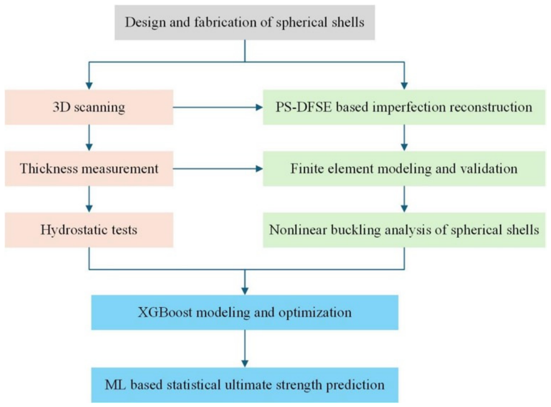
Although the ultimate strength of spherical shells and ML-based prediction have been separately investigated, a comprehensive framework that integrates high-fidelity parametric imperfection characterization with efficient ultimate strength prediction remains lacking. This gap hinders the reliable quantification of probabilistic bounds for structural capacity under realistic multi-source uncertain imperfections. This paper investigates the buckling behavior of spherical shells subjected to inherent stochastic imperfections by leveraging ML methodologies. The remainder of this paper is organized as follows. Section 2 introduces the material and methods used in this study. Section 3 focuses on experimental investigations, encompassing structural design, fabrication, geometric measurements, and hydrostatic testing. Section 4 details numerical simulations, including FE modeling and buckling analysis under both perfect and imperfect shell configurations. Section 5 establishes ML models to predict the mean and standard deviation of the ultimate strength, thereby bypassing computationally intensive FE simulations; based on these ML models, the bounds of the cumulative probability distributions for the ultimate strength are quantified. Finally, Section 6 concludes the paper. Overall, this study offers a robust methodology for predicting the ultimate strength of spherical shells under multi-source uncertain imperfections. The flow diagram of the research procedure is presented in Figure 1.

2. Materials and Methods

2.1. PS-DFSE Based Imperfection Construction of Spherical Shells

Initial imperfections, such as deformations induced by stamping and welding, have a pronounced impact on the buckling performance of spherical shells. Consequently, the actual ultimate strength of a spherical shell can be considerably lower than that of its idealized model. The ability to predict the ultimate strength and buckling performance of a spherical shell can be improved by properly introducing imperfections into the FEA model. To characterize the imperfections of spherical shells as accurately as possible, a method based on pole-smoothing double Fourier series expansion (PS-DFSE) is proposed.

2.1.1. Double Fourier Series Expansion with Pole Smoothing

Let ${\mathit{P}}_i={\left(x_i,y_i,z_i\right)}^{\mathrm{T}},(i=1,2,\dots ,N_{\mathrm{P}})$ denote the spatial coordinates of the scanned point cloud of a single spherical shell, where N_p represents the number of points in the cloud. To establish a local reference coordinate, an ideal sphere is first fitted using the linear least-squares method defined as following:

$$\min {\displaystyle \sum _{i=1}^{N_{\mathrm{P}}}{\left[{\left(x_i-x_0\right)}^2+{\left(y_i-y_0\right)}^2+{\left(z_i-z_0\right)}^2-R_{i\mathrm{n}}^2\right]}^2}$$

(1)

where ${\mathit{P}}_0={\left(x_0,y_0,z_0\right)}^{\mathrm{T}}$ denotes the fitted center of the reference sphere, and $R_{i\mathrm{n}}$ represents the corresponding radius of the ideal sphere.

According to the fitted center P₀, a local Cartesian coordinate system is established, and location of the point cloud is transformed as $X_i=x_i-x_0$, $Y_i=y_i-y_0$, $Z_i=z_i-z_0$. These coordinates are then converted to the spherical coordinate system to facilitate boundary series expansions over the entire surface:

$$\left\{\begin{array}{c}{r}_i=\sqrt{X_i^2+Y_i^2+Z_i^2}\\ {\theta }_i=\arccos \left({\displaystyle \frac{Z_i}{r_i}}\right),{\theta }_i\in \left[0,\pi \right]\\ {\phi }_i=\arctan 2\left(Y_i,X_i\right),{\varphi }_i\in \left[-\pi ,\pi \right]\end{array}\right.$$

(2)

where r_i represents the radial distance, θ_i denotes the colatitude angle, and φ_i is the azimuthal angle. The initial radial deviation of each point in the scanned point cloud is defined as:

$$\Delta r_i=r_i-R_{i\mathrm{n}}$$

(3)

To reconstruct the continuous spatial distribution of the radial deviation over the entire shell, a standard double Fourier series expansion is adopted to represent the continuous deviation field [41,42]:

$$\Delta r\left(\theta ,\phi \right)={\displaystyle \sum _{m=-M}^M{\displaystyle \sum _{n=-N}^N{C}_{m,n}{e}^{\mathrm{j}(m\theta +n\phi )}}}$$

(4)

where M and N represent the truncation orders in the θ- and φ-directions, respectively; C_m,n denotes the complex-valued Fourier coefficients; and j is the imaginary unit.

However, in standard spherical DFSE, the longitudinal coordinate φ suffers geometric degeneracy at the poles (θ → 0 and θ → π), i.e., where all meridians converge to a single physical point. Consequently, any term with a non-zero azimuthal frequency introduces multi-valuedness and high-frequency numerical oscillations, which manifest as petal-like radial artifacts around the polar regions. In order to restore physical single-valuedness and suppress non-physical polar fluctuations, a localized pole-smoothing weight is incorporated into each Fourier basis function. The refined PS-DFSE model for the imperfect spherical surface reconstruct can be written as:

$$\Delta r(\theta ,\phi )=\Re \left\{{\displaystyle \sum _{m=-M}^M{\displaystyle \sum _{n=-N}^N{C}_{m,n}{\left[\sin \left(\theta \right)\right]}^{\left|n\right|p}{e}^{\mathrm{j}(m\theta +n\phi )}}}\right\}$$

(5)

where $W_p\left(\theta ,n\right)={\left[\sin (\theta )\right]}^{\left|n\right|p}$ is the localized pole-smoothing weight, and p is the user-defined pole-smoothing index.

2.1.2. Parameter Calculation of PS-DFSE

To determine the optimal complex-valued Fourier coefficients C_m,n, the continuous PS-DFSE is discretized over the experimental scanned point cloud. By flattening the double summation index in Equation (6) into a single-column index, the complex design matrix $\mathit{A}\in {ℂ}^{N_{\mathrm{p}}\times K}$ can be constructed. The element of the design matrix corresponding to the ith point and the kth basis function is defined as follows:

$$A_{i,k}={\left[\max \left(\sin {\theta }_i,\delta \right)\right]}^{\left|n_k\right|\cdot p}{e}^{\mathrm{j}\left(m_k{\theta }_i+n_k{\varphi }_i\right)}$$

(6)

where δ is a minor threshold added to prevent numerical underflow at the absolute poles.

Given the experimental radial deviation vector $\mathit{y}={\left[\Delta r_1,\Delta r_2,\dots ,\Delta r_{N_p}\right]}^{\mathrm{T}}$ and the vector of undetermined complex-valued Fourier coefficients $\mathit{c}={\left[C_1,C_2,\dots ,C_K\right]}^{\mathrm{T}}$, the discrete radial deviation can be expressed as a linear system in the matrix form:

$$\mathit{A}\mathit{c}=\mathit{y}$$

(7)

The optimal coefficient vector in the above highly overdetermined system can be solved using the complex least-squares method via conjugate transpose as follows:

$$\mathit{c}={({\mathit{A}}^{\mathrm{H}}\mathit{A})}^{-1}{\mathit{A}}^{\mathrm{H}}\mathit{y}$$

(8)

2.1.3. Accuracy of Surface Reconstruction

Based on the calculated coefficient vector c, the continuous reconstructed deviation field can be mapped onto a regular curvilinear mesh. The reconstructed coordinate model of the imperfect spherical shell can be expressed as:

$$\left\{\begin{array}{l}{X}_{\mathrm{re}}(\theta ,\phi )=\left[R_{i\mathrm{n}}+\Delta r_{\mathrm{fit}}(\theta ,\phi )\right]\sin (\theta )\cos (\phi )+x_0\\ Y_{\mathrm{re}}(\theta ,\phi )=\left[R_{i\mathrm{n}}+\Delta r_{\mathrm{fit}}(\theta ,\phi )\right]\sin (\theta )\sin (\phi )+y_0\\ Z_{\mathrm{re}}(\theta ,\phi )=\left[R_{i\mathrm{n}}+\Delta r_{\mathrm{fit}}(\theta ,\phi )\right]\cos (\theta )+z_0\end{array}\right.$$

(9)

The reconstruction accuracy is evaluated using the root mean square error (RMSE_DFSE) and the coefficient of determination ($R_{\mathrm{DFSE}}^2$):

$$\left\{\begin{array}{l}{\mathrm{RMSE}}_{\mathrm{DFSE}}=\sqrt{{\displaystyle \frac{1}{N_p}}{\displaystyle \sum _{i=1}^{N_p}{\left(\Delta r_i-\Delta r_{\mathrm{fit}}({\theta }_i,{\phi }_i)\right)}^2}}\\ R_{\mathrm{DFSE}}^2=1-{\displaystyle \frac{{\displaystyle \sum _{i=1}^{N_p}{\left(\Delta r_i-\Delta r_{\mathrm{fit}}({\theta }_i,{\phi }_i)\right)}^2}}{{\displaystyle \sum _{i=1}^{N_p}{\left(\Delta r_i-\Delta \overline{r}\right)}^2}}}\end{array}\right.$$

(10)

where Δr_i and Δr_fit are the initial and fitted radial deviation, respectively, and $\Delta \overline{r}$ represents the mean value of the initial radial deviations. A high $R_{\mathrm{DFSE}}^2$ (close to 1) and a low RMSE_DFSE indicate that the PS-DFSE accurately captures the authentic spatial topology of the shell imperfections.

2.2. Structural Design and Fabrication

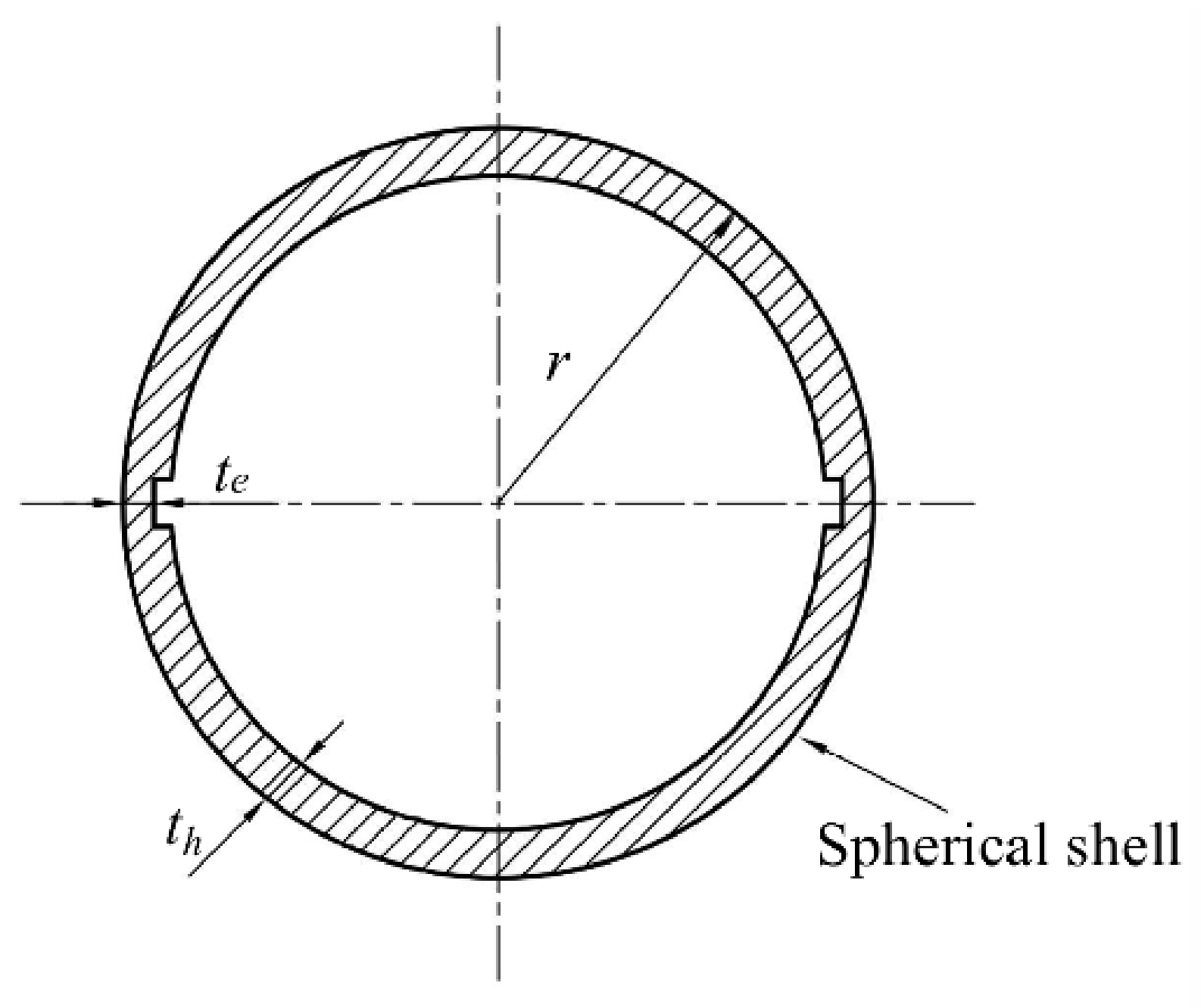
In consideration of ensuring test safety and minimizing measurement errors, the spherical shell was specified to have a nominal outer radius of r = 63 mm and a nominal thickness of 1 mm. Consequently, the thickness-to-radius ratio t/R was 1.59%, which falls within the range of thin-shell structures. However, due to welding effects, the thickness at the equatorial region is generally smaller than that of the hemispherical shell. The details of designed spherical shell are shown in Figure 2. In the figure, t_h denotes the wall thickness of hemispherical sections, while t_e corresponds to the thickness at the equatorial welding seam.

A total of thirty spherical shells were fabricated by welding pairs of stamped 304 stainless steel hemispheres, with the process meticulously controlled to ensure high-quality, reproducible joints. The hemispheres were produced through a stamping process: a flat circular blank is first cut and coated with lubricant, then clamped between a blank holder and a die while a punch presses the center downward into the die cavity. As the punch descends, the material flows radially inward and undergoes plastic deformation, gradually taking the shape of a hemisphere, with wrinkling controlled by the blank holder throughout. After forming, each hemisphere was polished along the equatorial edge.

The automated circumferential TIG welding method was then employed to assemble the hemisphere together due to its ability to produce precise welds with minimal heat input and distortion. High-purity argon (99.999%), delivered at a flow rate of 8–10 L/min, served as the shielding gas, creating an inert atmosphere to prevent the oxidation and contamination of both the weld pool and the heat-affected zone. A direct current, electrode negative of 45–55 A was applied, a range optimized for achieving adequate penetration and fusion of the material without introducing excessive thermal stresses, while the arc voltage was maintained at approximately 10–12 V. A controlled welding speed of 1.5–2.0 mm/s facilitated proper fusion and solidification characteristics of the weld bead, using a 1.6 mm diameter, 2% thoriated tungsten (EWTh-2) electrode, sharpened to a conical tip, for its stable arc characteristics. No filler material was used, as the hemispheres were designed for a precise butt joint, allowing for direct autogenous fusion of the base material. Prior to welding, the hemispheres underwent thorough cleaning with acetone to remove any surface contaminants or oils, and precise edge alignment was ensured to create a tight fit. Subsequent to welding, the shells were polished to enhance dimensional tolerances and alleviate stress concentrations. This was followed by a visual inspection to identify any potential defects, including porosity, cracks, or undercut. Furthermore, post-weld heat treatment was intentionally not applied, ensuring the preservation of the material’s original properties and preventing additional deformation.

3. Experimental Studies

This section details the experimental studies, encompassing structural design and fabrication, dimensional measurements, and hydrostatic testing. All of these experiments were conducted at the Provincial University Key Laboratory for Advanced Deep-Sea Mechanical Equipment, Zhenjiang, China.

3.1. Geometric Measurements

Despite meticulous stamping and welding of the hemispherical shells, fabrication-induced imperfections remain inevitable. If these imperfections are neglected during modeling, the predicted buckling behaviors will differ significantly from the actual structural responses [43]. Based on relevant literature and the authors’ experience, the primary structural imperfections mainly consist of geometric deviations and thickness variations. To account for the aforementioned structural imperfections, non-destructive three-dimensional (3D) scanning and thickness measurements were performed on all fabricated specimens.

3.1.1. 3D Scanning

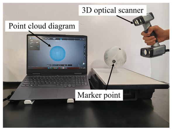
The external contours of spherical shells were characterized by 3D scanning, and the specific scanning measurement site is shown in Figure 3. First, a thin layer of white contrast enhancer was evenly sprayed onto the outer surface of all spherical shells to improve the contrast between the specimens and their background. Subsequently, several circular markers were randomly affixed to the surface to facilitate specimen positioning and subsequent data stitching. Then, a handheld dual-blue-light 3D scanner (Ein-Scan HX; SHINING 3D Tech. Co., Ltd., Hangzhou, Zhejiang, China) with a precision of 0.05 mm was used to scan each specimen comprehensively, and the corresponding three-dimensional point cloud was acquired. After scanning, the point cloud data were imported into the post-processing software Geomagic Studio (version 12) for coordinate registration and transformation. The processed point cloud data were employed in the subsequent FE modeling stage to map actual imperfections onto the ideal model, thereby improving the model fidelity. Meanwhile, the actual imperfect geometry of the spherical shells was reverse reconstructed, and an error analysis was conducted between the reconstructed imperfect surface and its corresponding ideal spherical surface.

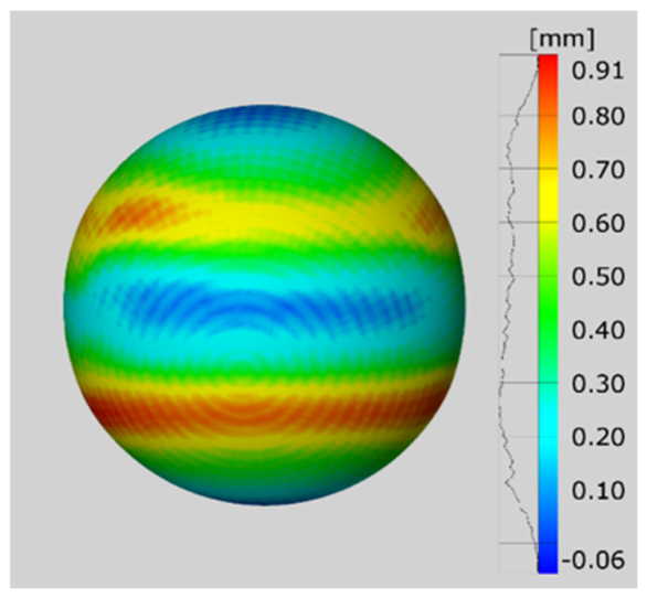
Figure 4 illustrates the radial deviation of a representative shell relative to its nominal geometry. As shown in the figure, the error manifests as circumferential concave and convex imperfections at the equator (welding seam) and at the mid-height of the two hemispherical shells. That is, the geometric imperfection and relief during the stamping and welding processes. In terms of error magnitude, the radial deviation was concentrated within the range of −0.06 mm to 0.91 mm, with positive values corresponding to convex imperfections and negative values to concave ones. It should be noted that the radial errors herein were compared against a spherical shell with a nominal diameter of 126 mm. The results dominated by positive errors indicate that the diameter of the formed spherical shell was slightly larger than its nominal diameter. All 30 spherical shells were fabricated and tested under identical processing conditions, and their geometric imperfections exhibited consistent characteristics across all specimens.

To quantify the geometric imperfections of a single spherical shell, radial errors between the measured point cloud and the nominal radius were calculated. The radial error of this point is:

$$W=\sqrt{x_{3\mathrm{D}}^2+y_{3\mathrm{D}}^2+z_{3\mathrm{D}}^2}-R_{\mathrm{n}}$$

(11)

where x_3D, y_3D, and z_3D are the position of the scanned point in the Cartesian coordinate system. W is the radial errors between the measured point and its nominal value. R_n is the nominal radius of the spherical shell, and R_n = 63 mm.

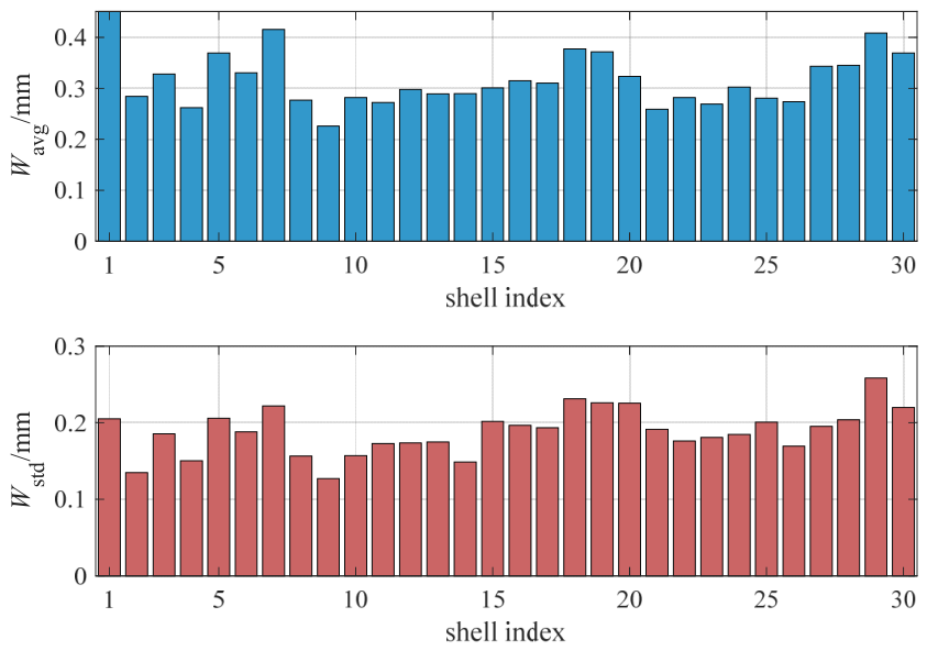
Additionally, the mean radial error (W_avg) and its standard deviation (W_std) were analyzed and presented in Figure 5 to characterize the average magnitude and dispersion of the errors. As illustrated in Figure 5, W_avg ranged from 0.2261 mm to 0.4509 mm, while W_std varied between 0.1270 mm and 0.2584 mm. The corresponding error-to-radius ratios were 0.359% and 0.716%, respectively, with the coefficient of variation spanning from 45.52% to 74.01%. These significant variations indicate that such geometric imperfections should be incorporated into the numerical model to ensure accurate predictions of the ultimate strength.

3.1.2. Thickness Measurement

The inherent slight thickness inhomogeneity of the hemispherical shell preform, together with the non-uniform material elongation during stamping, may lead to thickness variations in the final spherical shell. In addition, hemispherical shells can only be welded on their outer surface, leading to a different wall thickness in the welded zone relative to other regions. Therefore, the thickness of both the hemispherical shells and the weld seam was measured for each spherical shell to facilitate subsequent precise FE modeling.

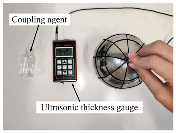
A non-destructive ultrasonic thickness gauge (DAKOTA/PX-7, Scotts Valley, CA, USA) with a precision of 0.002 mm was employed. The acoustic velocity of the gauge was calibrated to 5872 m/s prior to thickness measurement, based on a standard 304 specimen. Figure 6 shows the experimental setup of thickness measurement. Prior to the thickness measurement, a layer of general ultrasonic couplant was first applied to the gauge probe to enable efficient ultrasonic wave transmission and sufficient acoustic intensity at the specimen interface. Subsequently, a uniform grid of 42 test points, corresponding to seven meridional and eight parallel measurement lines, was marked on the outer surface of each spherical shell. To capture the equatorial welding seam, the measuring points were distributed in an odd-numbered pattern in the meridional direction. Finally, the probe was placed sequentially at each measurement point, and the corresponding thickness value was recorded.

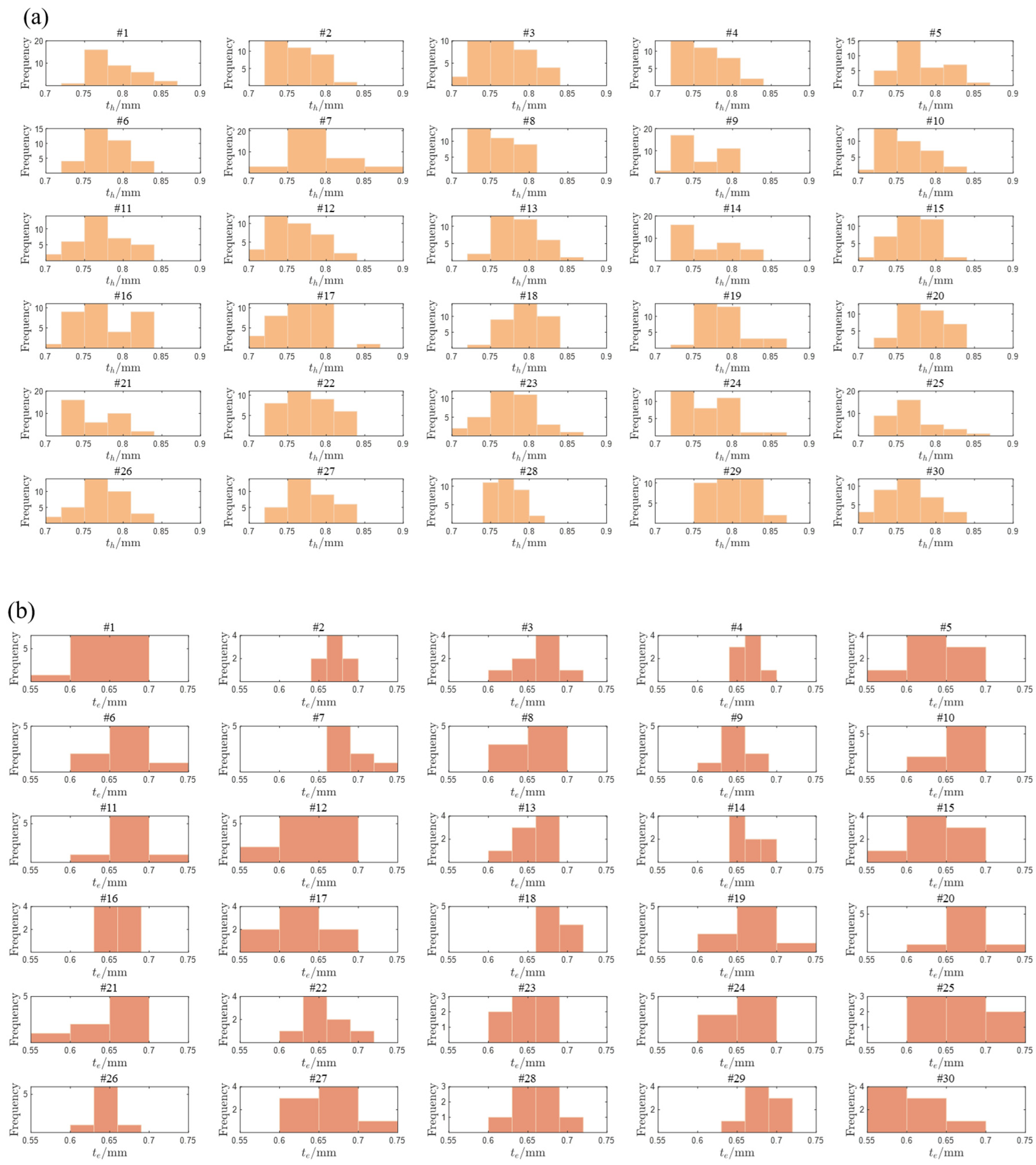
Figure 7 illustrates the frequency distributions of shell and equatorial thicknesses for all spherical shells. As shown in the figure, the thickness distribution over the hemispherical shell and equator cannot be accurately fitted using conventional distribution functions. This is mainly attributed to the non-uniform extension during stamping as well as non-uniform melting during welding. In addition, the limited number of test points also affects the distribution fitting. As a result, the thicknesses of the shell, including that on the hemispherical shell and equator, are treated as epistemic uncertainty and characterized by uniform distributions.

The statistical characteristics of the spherical shell thicknesses are summarized in

Table 1. Statistical characteristics of the spherical shell thicknesses.

Sample	Hemispherical Shell				Equator
	thmin/mm	thmax/mm	thavg/mm	thcov/%	temin/mm	temax/mm	teavg/mm	tecov/%
1	0.744	0.856	0.787	3.793	0.570	0.698	0.644	6.746
2	0.730	0.824	0.765	3.573	0.648	0.684	0.668	1.818
3	0.714	0.824	0.768	4.141	0.626	0.692	0.658	3.071
4	0.724	0.822	0.762	3.886	0.642	0.680	0.663	2.107
5	0.738	0.852	0.781	3.982	0.592	0.696	0.649	5.545
6	0.730	0.824	0.776	3.127	0.644	0.748	0.681	5.783
7	0.724	0.892	0.796	5.198	0.674	0.724	0.693	2.662
8	0.726	0.802	0.760	3.283	0.630	0.688	0.661	3.532
9	0.714	0.796	0.756	3.452	0.616	0.680	0.648	3.009
10	0.716	0.810	0.758	3.502	0.626	0.694	0.666	3.488
11	0.708	0.832	0.770	4.252	0.642	0.736	0.671	4.416
12	0.708	0.816	0.758	3.832	0.550	0.664	0.618	7.552
13	0.742	0.856	0.785	3.386	0.626	0.678	0.653	2.983
14	0.724	0.832	0.766	4.341	0.648	0.688	0.664	2.144
15	0.714	0.814	0.767	3.223	0.554	0.674	0.628	6.169
16	0.706	0.832	0.774	4.419	0.632	0.684	0.658	2.861
17	0.706	0.864	0.766	4.193	0.580	0.668	0.630	4.625
18	0.748	0.838	0.794	3.053	0.662	0.708	0.683	2.258
19	0.738	0.856	0.789	3.304	0.628	0.706	0.657	3.739
20	0.738	0.834	0.783	3.423	0.612	0.712	0.665	4.581
21	0.728	0.826	0.765	3.769	0.588	0.678	0.650	4.540
22	0.728	0.830	0.776	3.853	0.618	0.692	0.652	3.201
23	0.704	0.846	0.774	4.237	0.616	0.688	0.652	3.498
24	0.726	0.844	0.767	3.743	0.612	0.688	0.656	4.164
25	0.728	0.842	0.771	3.846	0.602	0.712	0.664	6.204
26	0.708	0.822	0.771	3.791	0.624	0.686	0.651	2.871
27	0.738	0.838	0.780	3.483	0.626	0.728	0.661	4.952
28	0.742	0.816	0.772	2.429	0.620	0.692	0.659	3.159
29	0.756	0.858	0.799	3.687	0.638	0.702	0.675	3.048
30	0.702	0.826	0.763	4.444	0.550	0.656	0.606	5.621

. As can be observed, the thickness ranges at the hemispherical shell and equator region varied among individual shells. Meanwhile, for a single spherical shell, the thickness at the equator was considerably smaller than that at the hemispherical shell. More specifically, the average thickness of the hemispherical shell ranged from 0.756 mm to 0.799 mm, whereas that of the equatorial region ranged from 0.606 mm to 0.693 mm. The average coefficients of variation for thickness in the hemispherical shells and equatorial region were 3.755% and 4.012%, respectively. These relatively large coefficients of variation indicate significant scatter in the shell thickness.

3.2. Hydrostatic Test

Spherical shells are commonly designed as structures capable of withstanding external pressure. The hydrostatic test is a high-fidelity experimental method to characterize the buckling performance of structures working in underwater service environments. The 30 spherical shells were tested in a hydrostatic pressure chamber with an inner diameter of 200 mm and a height of 400 mm. The maximum loading pressure was 40 MPa, much larger than the ultimate strength of designed spherical shells.

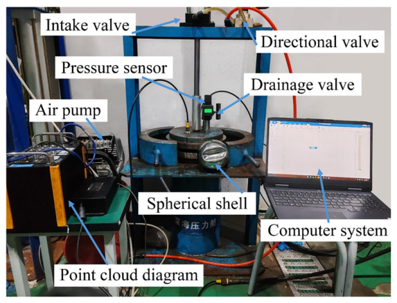
Figure 8 presents the experimental site of the hydrostatic test. The test specimen was first wrapped in a net bag and placed into the chamber to ensure it was submerged in water. Subsequently, the chamber cover was closed, and a manual hydraulic pump was used to slowly inject water and apply pressure into the chamber. The real-time pressure inside the chamber was monitored by a pressure sensor (SUP-P3000, Hangzhou, China) and recorded by a dynamic signal acquisition instrument (DH5902N; Donghua Test, Jingjiang, China) with a sampling frequency of 50 Hz. As the amount of water injected into the chamber increases, the external pressure acting on the spherical shell also gradually rises. When the pressure reaches a critical level, the spherical shell undergoes buckling failure, accompanied by a distinct bursting sound and a sudden decrease in chamber pressure. The maximum pressure recorded in the loading process indicates the ultimate strength P_cr of the shell.

Table 2. Ultimate strength of the spherical shells.

Sample	1	2	3	4	5	6	7	8	9	10
Pcr/MPa	5.307	6.201	6.956	6.343	7.328	6.462	6.523	6.578	5.609	6.132
Sample	11	12	13	14	15	16	17	18	19	20
Pcr/MPa	6.623	6.262	6.788	6.966	6.788	6.742	7.059	7.141	5.942	7.254
Sample	21	22	23	24	25	26	27	28	29	30
Pcr/MPa	6.236	6.658	6.709	6.803	7.065	7.453	7.329	6.489	6.639	6.555

shows the ultimate strength of all spherical shells. As indicated in the table, variations exist in the ultimate strength among these nominally identical spherical shells. The maximum and minimum ultimate strengths were 7.453 MPa and 5.307 MPa, respectively, with an average value of 6.631 MPa and a coefficient of variation of 7.348%. However, the maximum and minimum P_cr did not correspond to the shells with the maximum and minimum average thicknesses. This discrepancy is attributed to a combined effect of imperfections in the specimens. The hydrostatic test results are compared with numerical studies in Section 4.

4. Numerical Study

The buckling behavior of spherical shells considering multi-source imperfections was investigated through FE analysis, with experimental test results incorporated for modeling and validation. This section details the numerical studies, including FE modeling and imperfection reconstruction.

4.1. FE Modeling

To serve as a baseline for subsequent imperfection reconstruction, an ideal spherical shell that disregards geometric imperfections was established in the modeling stage. The FE model of the spherical shell was developed in Abaqus/CAE 2024, and its buckling behavior was analyzed using the nonlinear Riks method [44]. The entire modeling process was carried out in strict accordance with the specifications of the Chinese Classification Society (CCS) [45].

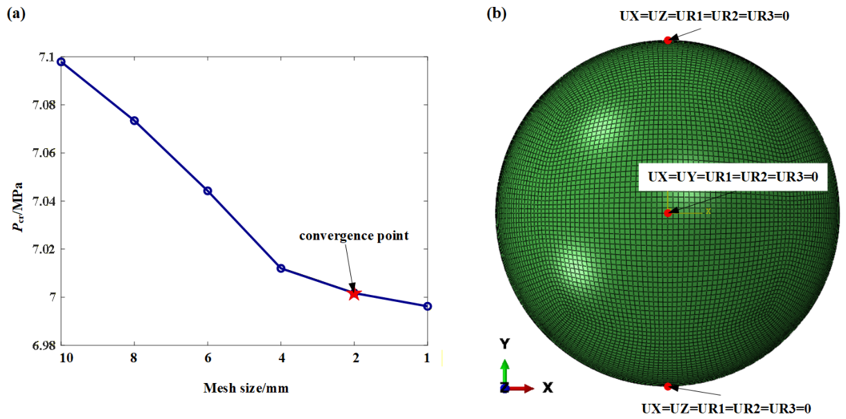
The spherical shell was modeled using S4R reduced-integration shell elements, which were employed for their ability to optimally balance modeling precision and computational cost. A mesh size of 2 mm was determined based on a mesh convergence analysis, as illustrated in Figure 9a. To facilitate the subsequent mapping of 3D scanning results onto the FE model, the external surface was defined as the reference surface during the modeling phase, and an inward offset was applied to define the thickness of hemispherical shells and equator. For comparative analysis against the defect reconstruction results obtained later, the thickness on the hemispherical shells and equator were initially configured as the average of shell #1, i.e., 0.787 mm and 0.644 mm, respectively.

The spherical shells were made of 304 stainless steel, and many studies have indicated that the stress–strain curve of this material is bilinear. As a result, an idealized elastic–plastic material constitutive model was employed. The material properties configured in the model, including elastic modular E = 206 GPa, Poisson’s ration μ = 0.3, and yielding strength σ_y = 310 MPa, were provided by the manufacturer.

A uniformly distributed external pressure was applied to the outer surface of the spherical shell to simulate the experimental scenario. Along one meridian of the spherical shell, three nodes were constrained to suppress rigid-body motion: (1) the two poles were fixed in the Y- and Z-directions and in all three rotational degrees of freedom (U2 = U3 = UR1 = UR2 = UR3 = 0); (2) the equatorial intersection point of the same meridian was fixed in the X- and Y-directions and in all three rotational degrees of freedom (U1 = U2 = UR1 = UR2 = UR3 = 0). Collectively, these three sets of constraints eliminate all six rigid-body modes while leaving the shell free to deform radially.

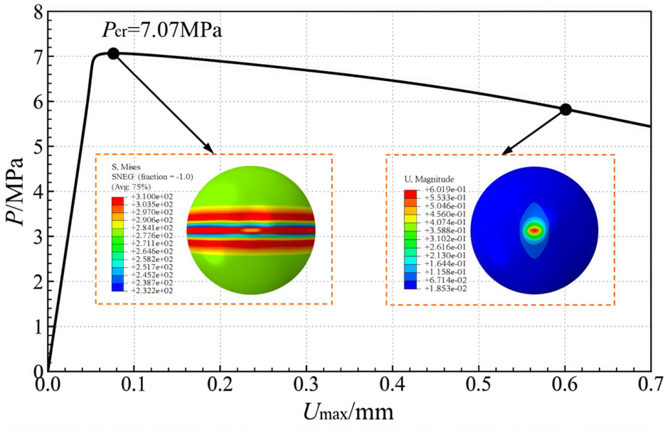
Based on the established FE model, nonlinear buckling analysis was performed to obtain the nonlinear equilibrium path and failure pressure of the spherical shell. The arc-length method was employed to control the load incremental parameters and ensure the stability of the numerical model. Specifically, the initial arc increment was set as 0.01, and the minimum and maximum arc increment were set as 1 × 10⁻⁵ and 0.1, respectively. During the solution process, the arc length was adjusted automatically to trace the structure’s equilibrium path. As a result, the load proportionality factor (LPF) curve, plotting the applied pressure against the maximum displacement, is displayed in Figure 10. As shown in the figure, the peak of the LPF curve defines the structural ultimate strength, yielding a maximum collapse pressure of 7.07 MPa for the spherical shell.

4.2. Geometric Imperfections Reconstruction of Spherical Shells

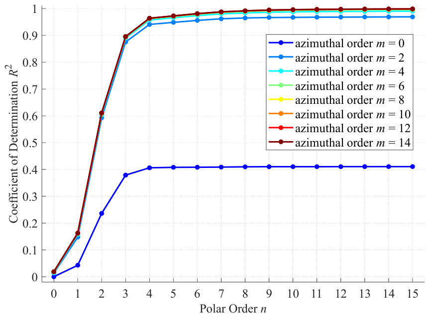
The geometric imperfections of all tested spherical shells were reconstructed, and their fitting accuracy was verified. Taking shell #1 as an example, Figure 11 presents the fitting errors between the original point cloud and the imperfect surface reconstructed using the PS-DFSE method. As illustrated, the reconstruction accuracy improved with higher polar and azimuthal truncation orders. For shell #1, the truncation orders converged at m = 6 (polar) and n = 8 (azimuthal), beyond which no significant improvement in fitting accuracy was observed. Parallel analyses were conducted on the remaining 29 shells. To ensure that the fitting accuracy of all 30 spherical shells uniformly exceeded 0.985, the conservative truncation orders of m = 10 and n = 8 were ultimately selected for the entire dataset. Finally, a total of thirty complex-valued column vectors were obtained, each encoding the Fourier coefficients that characterize the imperfection field of a single measured shell. These vectors were assembled column by column into a 357 × 30 matrix, denoted as C_all.

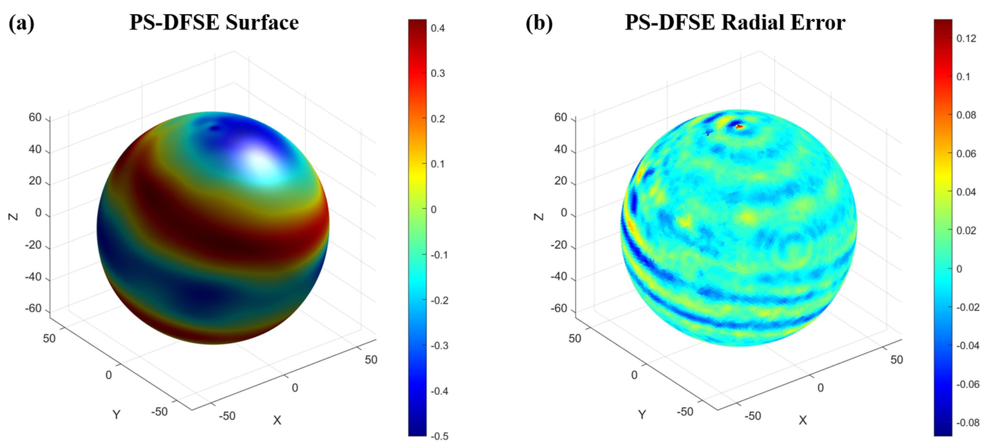
Figure 12 presents the radial deviations of the reconstructed imperfect spherical shell (using the PS-DFSE method) relative to both the ideal sphere and the original point cloud. As illustrated, the radial deviation between the imperfect and ideal spherical surfaces ranged from −0.5 mm to 0.4 mm, indicating a pronounced geometric imperfection in the radial direction. In contrast, the radial error between the reconstructed surface and the initial scanned point cloud was confined to a much smaller range of −0.08 mm to 0.12 mm. This substantial reduction in radial error demonstrates that the PS-DFSE reconstructed surface can accurately represent the scanned physical shell.

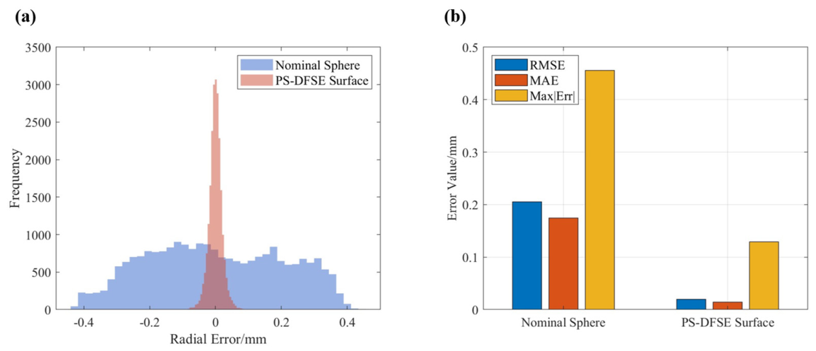
Furthermore, the statistical characteristics of the radial deviations shown in Figure 13 indicate that the PS-DFSE reconstructed imperfect shell achieved a much higher fitting accuracy than the nominal ideal shell. Specifically, the distribution histogram of radial deviations in Figure 13a demonstrates that the radial errors of the reconstructed shell closely followed a normal distribution, with a remarkably small standard deviation of σ = 0.0195 mm. Compared to the deviations of the nominal shell relative to the point cloud (σ = 0.205 mm), the reconstructed shell exhibited a much tighter error distribution, highlighting a significantly lower dispersion of radial errors. Meanwhile, the quantitative metrics presented in Figure 13b further confirm this superior accuracy. Specifically, the root mean squared error (RMSE_DFSE) decreased from 0.205 mm to 0.0195 mm, the mean absolute error (MAE_DFSE) dropped from 0.1749 mm to 0.0146 mm, and the maximum absolute error (Max|Err|) was reduced from 0.4553 mm to 0.1293 mm. Such a substantial reduction across all key metrics demonstrates that the geometric deviations of the reconstructed imperfect shell from the scanned point cloud were minimized to an extremely low level.

4.3. Ultimate Strength Prediction of Imperfect Spherical Shell

By utilizing the PS-DFSE method, the reconstructed imperfect geometry can be seamlessly mapped onto FE models to enhance simulation accuracy. Taking shell #1 as an example, the coefficient vector c was first calculated based on the scanned point cloud, with the polar and azimuthal truncation orders set to m = 10 and n = 8, respectively. Subsequently, a continuously reconstructed deviation field was generated via the PS-DFSE method, which was then used to update the nodal coordinates of the perfect FE model established in Section 4.1. Finally, the ultimate strength of the spherical shell incorporating the reconstructed geometric imperfections was predicted. To account for the localized effects of welding on material properties, the yield strength of elements within the equatorial region was treated as an independent parameter, assigned as σ_y2 = 250 MPa in the model. The remaining material properties were defined as identical to those of the 304 stainless steel.

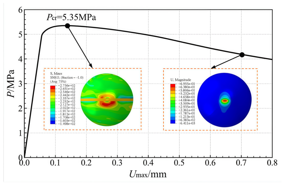
The load–displacement equilibrium path of spherical shell #1 is presented in Figure 14, where the horizontal and vertical axes denote the maximum displacement and the applied external pressure, respectively. As illustrated, the maximum displacement initially increases linearly with the external pressure, followed by a nonlinear transition near the peak of the curve, which is attributed to material plasticity and large geometric deformations. The peak of this curve, representing the maximum external pressure sustained, identifies the ultimate strength (P_cr = 5.35 MPa). Beyond this peak, the external pressure drops while the maximum displacement continues to grow, signifying shell collapse and a degraded residual load-bearing capacity. Meanwhile, the stress and displacement contours in Figure 14 demonstrate that localized dimpling first initiates at the weld seams of the shell, subsequently propagates toward the polar hemispheres, and ultimately forms a localized dent spanning the equator. This predicted collapse mode of the spherical shell agrees well with experimental observations. Furthermore, the numerical error was merely 0.81%, representing a significant improvement over the perfect model, which yielded a prediction error of 33.22%. The consistent collapse mode and remarkably low prediction error demonstrate that the FE model incorporating PS-DFSE reconstructed imperfections possesses high geometric fidelity and can accurately capture the actual physical state of the structure.

5. Results and Discussion

This section investigates the ML-based prediction of the statistical properties governing the ultimate strength of spherical shells. First, a stochastic dataset was constructed using FEMs that incorporated PS-DFSE reconstructed geometric imperfections. Subsequently, the XGBoost models were trained, with its hyperparameters optimized via Optuna. Through this process, the mapping relationship between variable structural/material parameters and the resulting statistical properties of the ultimate strength was established. Finally, the probabilistic bounds of the ultimate strength for this batch of imperfect spherical shell samples were predicted.

5.1. Database Establishment

The thicknesses of the hemispherical shells (t_h) and the equator region (t_e), along with the equivalent yield strength of elements in the equator region (σ_y2), were considered as the uncertain input parameters. As shown in Figure 7, the measured thickness $t_h$ ranged from 0.702 mm to 0.892 mm, and $t_e$ ranged from 0.550 mm to 0.748 mm. Consequently, the parameter ranges designed for constructing the database were set to 0.7 mm~0.9 mm for t_h and 0.55 mm~0.75 mm for $t_e$. Additionally, to account for the effects of welding on the material properties in the equator region, the equivalent yield strength σ_y2 was varied from 250 MPa to 400 MPa. Latin hypercube sampling (LHS) was employed to generate samples within these predefined ranges, yielding 800 samples for model training and 80 samples for testing.

For each sampled combination of shell thickness and equivalent yield strength σ_y2, a series of parametric FE models of imperfect spherical shells were randomly generated based on the PS-DFSE fitting results of the 30 experimental spherical shells, and the corresponding ultimate loads of the spherical shells were calculated. The generation procedure was as follows. First, the real and imaginary parts of the previously assembled matrix C_all were concatenated to form a real-valued data matrix Q = [Re(C_all)^T, Im(C_all)^T]. The column mean coefficient vector q was then calculated across all 30 shells, and the data were centered as Q_cen = Q − q. PCA was subsequently performed via the economy-size SVD of the centered data matrix Q_cen = USV^T, where V contains the principal directions and the singular values s_i on the diagonal of S are relate to the eigenvalues of the covariance matrix as ${\lambda }_i=s_i^2/29,i=1,2,\dots ,30$. All 30 principal components were retained, accounting for the cumulative variance in the empirical coefficient data. This truncation filters out high-order modes that predominantly represent measurement noise while preserving the dominant geometric features of the measured imperfections.

A new random coefficient vector q_new was generated as ${\mathit{q}}_{\mathrm{new}}=\mathit{q}+\mathit{V}\left(\sqrt{\mathit{\lambda }}\odot {\mathit{Z}}_r\right)$, where the eigenvalue vector is $\mathit{\lambda }={\left[{\lambda }_1,{\lambda }_2,{\lambda }_3,\dots ,{\lambda }_{30}\right]}^{\mathrm{T}}$, Z_r is a vector of independent standard normal random variables, and $\odot$ denotes element-wise multiplication. This formulation implicitly assumes that the coefficient vectors in the principal component space follow a multivariate normal distribution. The validity of this assumption was verified by examining the marginal distributions of the experimental coefficients projected onto the leading principal axes, which exhibited approximately elliptical symmetry consistent with normality. This formulation ensures that the generated coefficients preserve both the mean vector and the covariance structure of the original empirical distribution; q_new thus constitutes a random realization within the principal subspace, with the variance along each principal axis scaled to match that of the experimental data.

Finally, the real-valued vector q_new was partitioned back into its real and imaginary halves to recover the complex PS-DFSE coefficient vector as ${\mathit{c}}_{new}={\mathit{q}}_{new,1:357}+\mathit{i}{\mathit{q}}_{new,358:714}$. Based on the randomly generated coefficient vector, the geometric imperfection was reconstructed and mapped onto the FE model, and the ultimate strength of the resulting imperfect spherical shell was calculated.

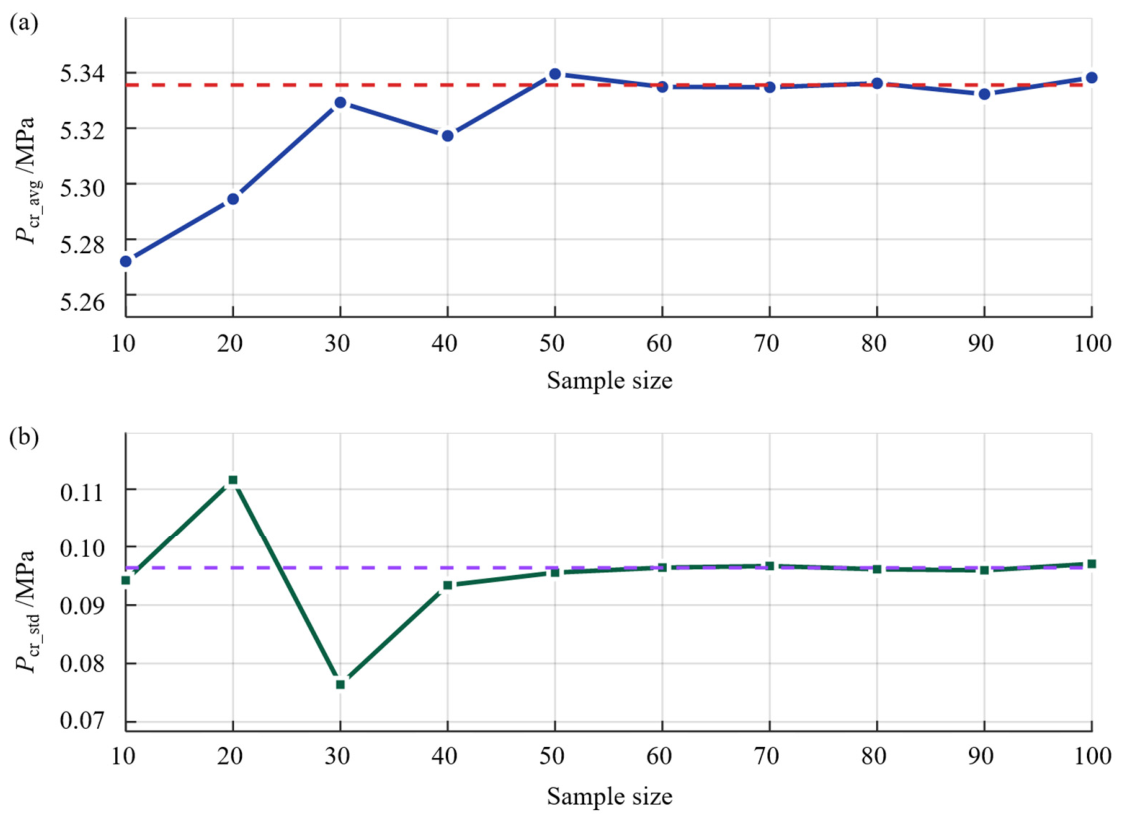
The above process was repeated 50 times for each combination of thickness and equivalent yield strength, and the mean and standard deviation of the ultimate strength across these 50 imperfect spherical shells were calculated. The sample size for geometric imperfection reconstruction for each combination of thickness and equivalent yield strength was determined through a convergence study. For a representative combination of shell thickness and equivalent yield strength, the mean and standard deviation of the ultimate strength were computed for sample sizes ranging from N_s = 10 to N_s = 100 with an increment of 10. The variations of both mean and standard deviation of the ultimate strength with the sample size of geometric imperfections are shown in Figure 15. It can be observed that both the mean and standard deviation converged after approximately 50 realizations.

5.2. ML Modelling

5.2.1. ML Models

Two independent regression tasks were established to predict the mean and standard deviation of the ultimate strength P_cr for spherical shells with uncertain imperfections. The dataset was structured as tabular data, with rows representing individual samples and columns corresponding to input features or target statistical moments. Each sample comprised a specific combination of weld yield strength, shell thickness, and weld thickness. Given the structured nature of the data and the strong nonlinear coupling between inputs and outputs, XGBoost was selected as the primary prediction model, complemented by several benchmark models from different algorithmic families for comparative evaluation.

XGBoost, short for extreme gradient boosting, is an advanced ensemble learning framework specifically designed for tabular data, offering both high computational efficiency and predictive performance [46]. It builds decision trees sequentially in a gradient boosting fashion, where each new tree fits the residuals of the previous ensemble, progressively refining prediction accuracy. For the two regression tasks in this study, this mechanism offers two key benefits. First, it accurately captures the high-order nonlinear mapping between geometric/material parameters and the mean ultimate strength P_{cr_avg}, achieving precise regression for this large-magnitude target. Second, it maintains stable fitting performance for the standard deviation P_{cr_std}, a small-magnitude target with a narrow numerical range, effectively avoiding the scale-induced bias commonly observed in linear models or neural networks. To ensure robust generalization under complex imperfection interactions, XGBoost incorporates both L1 and L2 regularization terms to penalize model complexity and mitigate overfitting on the finite-element-derived dataset. Furthermore, its parallelized tree construction enables rapid training and efficient hyperparameter search without sacrificing accuracy. Detailed theoretical foundations of XGBoost can be found in the original literature [46].

Given the substantial influence of hyperparameter configurations on XGBoost’s performance, hyperparameter optimization was conducted separately for the two regression tasks using Optuna [47]. Compared to grid search or random search, Optuna offers superior efficiency and solution quality. It adaptively prunes underperforming trials during optimization, focusing computational resources on promising hyperparameter regions and accelerating convergence. Its tree-structured Parzen estimator enables intelligent sampling of the predefined search space, reliably identifying near-optimal configurations with fewer trials.

To establish a comprehensive performance baseline, benchmark models from three major families were selected. Classical models, including elastic net, polynomial regression, support vector regression (SVR), and k-nearest neighbors (KNN), were chosen to represent linear and conventional nonlinear regression. Tree-based ensemble models, specifically random forest (RF) and light gradient boosting machine (LightGBM), were adopted as peer benchmarks to XGBoost. In addition, a backpropagation neural network (BPNN) was constructed to examine the performance of connectionist learning methods on this tabular regression task. This multi-model comparison also serves to quantify the nonlinear complexity of the underlying mapping. All models were trained and tested on identical datasets to ensure a fair evaluation, with detailed performance comparisons presented in the following sections.

5.2.2. Performance Evaluation Metrics

Four metrics were used to objectively evaluate the ML models’ predictive performance for the mean and standard deviation of spherical shell ultimate strength: the coefficient of determination (R²), root mean squared error (RMSE), mean absolute error (MAE), and mean absolute percentage error (MAPE). The mathematical formulations for R², RMSE, MAE, and MAPE are given in Equations (12)–(15), respectively [39]. R² quantifies the proportion of variance in the target statistical characteristic of ultimate strength that can be explained by the model, with values closer to 1 indicating superior predictive ability. The RMSE represents the square root of the average of squared differences between the predicted and ground-truth values, and a smaller RMSE indicates better model fit. The MAE is the average of the absolute differences between the two sets of values, with smaller values reflecting higher prediction accuracy. Finally, the MAPE expresses the average absolute error as a percentage, offering intuitive insight into relative deviations.

$$R^2=1-{\displaystyle \frac{{\displaystyle \sum _{i=1}^n{\left(y_i-{\widehat{y}}_i\right)}^2}}{{\displaystyle \sum _{i=1}^n{\left(y_i-\overline{y}\right)}^2}}}$$

(12)

$$\mathrm{RMSE}=\sqrt{{\displaystyle \frac{1}{n}}{\displaystyle \sum _{i=1}^n{\left(y_i-{\widehat{y}}_i\right)}^2}}$$

(13)

$$\mathrm{MAE}={\displaystyle \frac{1}{n}}{\displaystyle \sum _{i=1}^n\left|y_i-{\widehat{y}}_i\right|}$$

(14)

$$\mathrm{MAPE}={\displaystyle \frac{100\%}{n}}{\displaystyle \sum _{i=1}^n\left|\frac{y_i-{\widehat{y}}_i}{y_i}\right|}$$

(15)

where n denotes the total number of samples; y_i is the ground-truth value of the target either P_{cr_avg} or P_{cr_std} obtained from stochastic FE simulations; ${\widehat{y}}_i$ is the corresponding model-predicted value; $\overline{y}$ represents the sample mean of the ground-truth target values.

5.2.3. Hyperparameter Optimization

The predictive performance of XGBoost is highly sensitive to its hyperparameter configuration. To maximize generalization capacity on unseen data and mitigate overfitting, hyperparameters were optimized separately for the P_{cr_avg} and P_{cr_std} prediction models using Optuna [47]. During hyperparameter optimization, the training set was further partitioned into training and validation subsets at a ratio of 9:1. The optimization objective was defined as maximizing the R² on the validation set. This objective prioritizes out-of-sample predictive power over mere memorization of training samples. Moreover, as a normalized metric, R² eliminates the influence of target variable magnitude, enabling a fair comparison of optimization effects across the two prediction tasks that differ substantially in numerical scale. To prevent data leakage, the hyperparameter tuning procedure was conducted exclusively on the training data, with the independent test set withheld from any parameter search process.

A total of 80 Optuna trials were executed to search the predefined hyperparameter space for seven core XGBoost hyperparameters controlling model complexity, learning dynamics, and regularization intensity. An identical search space was applied to both prediction tasks to maintain consistency. The search ranges and the optimal values identified for each model are summarized in

Table 3. Hyperparameter search ranges and optimal configurations for XGBoost models predicting P_{cr_avg} and P_{cr_std.}

Hyperparameter	Type	Search Range	Optimal Value (Pcr_avg)	Optimal Value (Pcr_std)
Number of estimators	Integer	[100, 1000], step = 50	950	600
Maximum tree depth	Integer	[3, 12]	3	8
Learning rate	Float	[0.01, 0.3]	0.064	0.026
Subsample ratio	Float	[0.6, 1.0]	0.808	0.744
Column subsample ratio	Float	[0.6, 1.0]	0.754	0.845
L1 regularization weight	Float	[1 × 10−4, 10.0]	0.095	1.902 × 10−4
L2 regularization weight	Float	[1 × 10−4, 10.0]	3.896	1.767 × 10−3

. The optimal validation-set R² values achieved were 0.9926 for the P_{cr_avg} model and 0.9123 for the P_{cr_std} model, indicating excellent predictive performance for both tasks.

The optimal hyperparameter configurations exhibited a clear divergence between the two models. The P_{cr_std} prediction model favors a deeper tree structure (maximum tree depth = 8) and a smaller learning rate (0.026), which endows it with enhanced nonlinear fitting capacity to capture the intricate variations in ultimate strength dispersion induced by random geometric imperfections. In contrast, the P_{cr_avg} model adopts shallower trees (maximum tree depth = 3) together with substantially stronger L1 and L2 regularization (L1 regularization term on weights = 0.095, L2 regularization term on weights = 3.89), effectively suppressing overfitting for the relatively smooth monotonic mapping between structural parameters and mean bearing capacity. This marked discrepancy further substantiates the rationale for establishing two independent regression models rather than a single multi-output predictor. Notably, the hyperparameters of all benchmarked models were also optimized. This approach ensured a comprehensive and fair comparison of all modeling methods.

5.2.4. Performance Validation

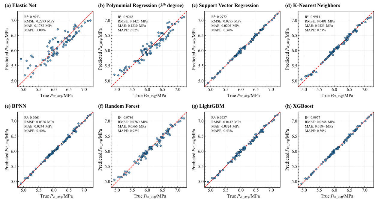
The XGBoost model and all benchmark models were retrained on the complete training set using their respective optimal hyperparameters, and their predictive performance was evaluated on the independent test set. The predictive performance of all models for the P_{cr_avg} prediction is visualized in Figure 16 and quantitatively summarized in

Table 4. Performance metrics of P_{cr_avg} prediction models on the test set.

Model	R2	RMSE/MPa	MAE/MPa	MAPE
Elastic net	0.8053	0.2293	0.1782	3.00%
Polynomial regression (3th degree)	0.9248	0.1425	0.1230	2.02%
SVR	0.9972	0.0275	0.0206	0.34%
KNN	0.9914	0.0481	0.0325	0.53%
BPNN	0.9961	0.0326	0.0244	0.40%
Random forest	0.9786	0.0760	0.0566	0.92%
LightGBM	0.9937	0.0412	0.0324	0.53%
XGBoost	0.9977	0.0248	0.0184	0.30%

.

The XGBoost model outperformed all benchmark models, achieving the highest R² of 0.9977, the lowest RMSE of 0.0248 MPa, the lowest MAE of 0.0184 MPa, and the lowest MAPE of 0.30%. Its superior performance is intuitively illustrated in the XGBoost scatter plot in Figure 16, where the data points are tightly clustered around the diagonal line, indicating minimal prediction errors. In contrast, the scatter plots for other models, especially the elastic net and polynomial regression models contained more-scattered data points, consistent with their lower R² and higher error values. Therefore, XGBoost was selected as the primary model for predicting the mean ultimate strength P_{cr_avg} of spherical shells.

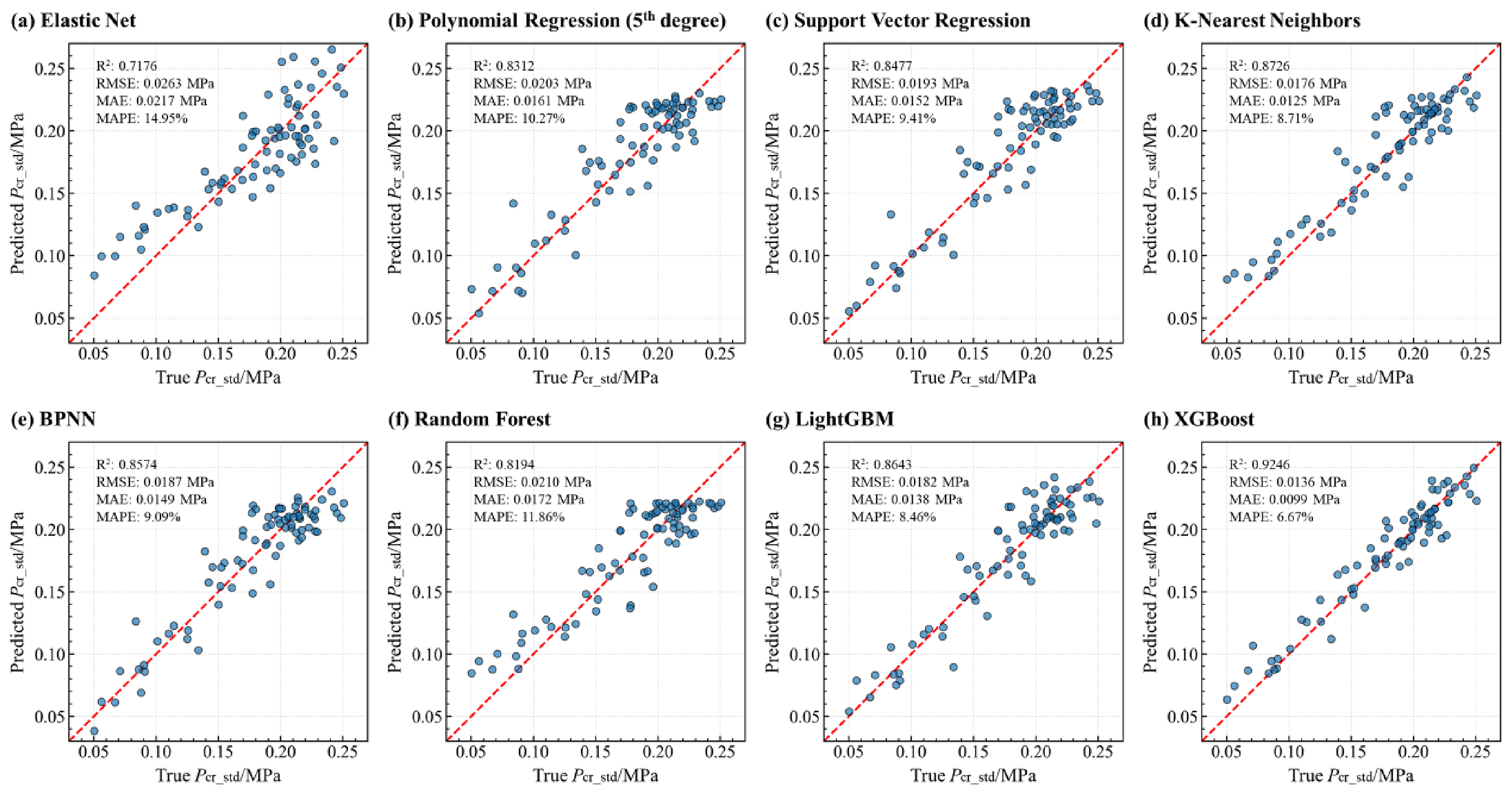
The predictive performance of all models for the P_{cr_std} task is summarized in

Table 5. Performance metrics of P_{cr_std} prediction models on the test set.

Model	R2	RMSE/MPa	MAE/MPa	MAPE
Elastic net	0.7176	0.0263	0.0217	14.95%
Polynomial regression (5th degree)	0.8312	0.0203	0.0161	10.27%
SVR	0.8477	0.0193	0.0152	9.41%
KNN	0.8726	0.0176	0.0125	8.71%
BPNN	0.8574	0.0187	0.0149	9.09%
Random forest	0.8194	0.0210	0.0172	11.86%
LightGBM	0.8643	0.0182	0.0138	8.46%
XGBoost	0.9246	0.0136	0.0099	6.67%

and visualized in Figure 17. The results revealed a similar performance hierarchy among the models, though the overall accuracy was notably lower than that for the P_{cr_avg} task. This is expected, as predicting the standard deviation is inherently more challenging due to its high sensitivity to the complex interactions of random geometric imperfections. The elastic net model was the lowest-performing model, confirming that linear models are incapable of characterizing the intricate relationships governing the dispersion of ultimate strength. The polynomial regression model was a marginal improvement over the linear model, but its fixed-order expansion remained insufficient for capturing the high-dimensional nonlinearity involved. The random forest model exhibited moderate predictive capability, which was inferior to other ensemble models, indicating that the bagging mechanism is less effective than boosting for this challenging task. The SVR, KNN, BPNN, and LightGBM models achieved relatively satisfactory performance, with R² values exceeding 0.84 and MAPE below 9.5%.

Notably, the XGBoost model outperformed all benchmark models, achieving the highest R² of 0.9246, the lowest RMSE of 0.0136 MPa, the lowest MAE of 0.0099 MPa, and the lowest MAPE of 6.67%. Its superior performance is intuitively illustrated in the XGBoost scatter plot in Figure 17, where the data points exhibited the most concentrated distribution along the diagonal line. The superior performance of XGBoost can be attributed to its gradient boosting framework, which progressively fits residuals to capture high-order nonlinear interactions, along with its built-in regularization that effectively mitigates overfitting on the finite-element-derived dataset. Therefore, XGBoost was selected as the primary model for also predicting the standard deviation of ultimate strength.

5.3. Prediction of Ultimate Strength Probabilistic Bounds

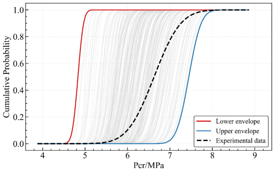
According to the thickness measurements shown in Figure 6, the thicknesses of the hemispherical shells and the equator region could not be adequately fitted by any standard probability distribution. Consequently, they were treated as interval variables, with ranges identical to those used for database construction. A total of 200 uniform samplings in the above ranges were conducted, and the mean and standard deviation of ultimate strength of each sample were predicted based on the XGBoost models.

Figure 18 presents the cumulative distribution functions (CDFs) of the ultimate strength for the spherical shells. As shown in the figure, the experimental CDF of the ultimate strength lies within the lower and upper bounds of the predicted CDFs. For the lower envelope, the mean and standard deviation were 4.833 MPa and 0.105 MPa, respectively, while those for the upper envelope were 7.446 MPa and 0.228 MPa. The differences in the mean and standard deviation between the lower and upper envelopes were 2.613 MPa and 0.123 MPa, respectively. Compared with the experimental results (mean of 6.627 MPa and standard deviation of 0.495 MPa), the ML-based prediction of the ultimate strength CDF envelope successfully encompassed the experimental data. At a confidence level of 99.74%, the margin of the upper bound prediction was 0.018 MPa, and the margin of the lower bound prediction was 0.624 MPa. The confidence interval was calculated under the normality assumption, a convention widely adopted in engineering for establishing conservative design limits. The confidence interval derived under this assumption is wider than the spread of the experimental data alone, and the resulting bounds are therefore more conservative—ensuring that the predicted ultimate strength limits remain reliable for design reference.

6. Conclusions

This study investigated the statistical ultimate strength prediction of spherical shells with multi-source imperfections. The PS-DFSE method was adopted to reconstruct the geometric imperfections, and reconstruction accuracy was verified through experimental tests. A database of imperfection and the corresponding characteristics of ultimate strength was established through LHS, and two XGBoost models were trained and validated. Finally, the bounds of CDFs for ultimate strength were determined. The main conclusions as listed as follows.

(1)

The deviations of thickness and geometric shapes of spherical shells with nominal dimensions were obvious. The ultimate strength of spherical shell ignoring all imperfections was about 33.22% higher than its experimental value.

(2)

The PS-DFSE method can reconstruct geometric imperfections with high accuracy. The conservative truncation orders of m = 10 (polar) and n = 8 (azimuthal) could represent all 30 test spherical shells with a fitting accuracy exceeding 0.985.

(3)

The developed ML framework accurately predicted both the mean and standard deviation of spherical shell ultimate strength. The implemented XGBoost models consistently demonstrated superior performance, achieving a high R² of 0.9977 for the mean prediction and 0.9246 for standard deviation.

(4)

The reliability of the statistical ultimate strength predictions was validated, with the experimental CDF falling within the calculated lower and upper bounds of the predicted CDFs. At a confidence level of 99.74%, the margin of the upper bound prediction was 0.018 MPa, and the margin of the lower bound prediction was 0.624 MPa.

This study presents an innovative framework for the design and in-service maintenance of underwater equipment. Acknowledging a current limitation, the model assumed uniform shell thickness, thereby not fully capturing its spatial variability. Future research will endeavor to develop a more comprehensive model that incorporates broader uncertainties, such as material anisotropy and process-induced non-uniform thickness, to quantify their effects on buckling performance. Additionally, given that this research focused on a specific shell geometry and material, further validation is crucial to ascertain the adaptability of the proposed method across diverse dimensional and material configurations.

References

1. Zheng, J.; Zhao, M. Fluid-Structure Interaction of Spherical Pressure Hull Implosion in Deep-Sea Pressure: Experimental and Numerical Investigation. Ocean Eng. 2024, 291, 116378. [Google Scholar] [CrossRef]
2. Wang, F.; Wang, K.; Cui, W. A Simplified Life Estimation Method for the Spherical Hull of Deep Manned Submersibles. Mar. Struct. 2015, 44, 159–170. [Google Scholar] [CrossRef]
3. Pranesh, S.B.; Sathianarayanan, D.; Ramadass, G.A. Design Standards for Steel Spherical Pressure Hull for a Manned Submersible. J. Ocean Eng. Mar. Energy 2022, 8, 137–151. [Google Scholar] [CrossRef]
4. Ismail, M.S.; Mahmud, J.; Jailani, A. Buckling of an Imperfect Spherical Shell Subjected to External Pressure. Ocean Eng. 2023, 275, 114118. [Google Scholar] [CrossRef]
5. Pan, B.; Cui, W. An Overview of Buckling and Ultimate Strength of Spherical Pressure Hull under External Pressure. Mar. Struct. 2010, 23, 227–240. [Google Scholar] [CrossRef]
6. Zoelly, R. Über ein Knickungsproblem an der Kugelschale. Ph.D. Thesis, ETH Zurich, Zurich, Switzerland, 1915. [Google Scholar]
7. Bijlaard, P.P. Theory and Tests on the Plastic Stability of Plates and Shells. J. Aeronaut. Sci. 1949, 16, 529–541. [Google Scholar] [CrossRef]
8. NASA. Buckling of Thin-Walled Doubly Curved Shells; NASA SP-8032; NASA: Washington, DC, USA, 1969.
9. Hutchinson, J.W. Buckling of Spherical Shells Revisited. Proc. R. Soc. A Math. Phys. Eng. Sci. 2016, 472, 20160577. [Google Scholar] [CrossRef]
10. Koiter, W.T. The Nonlinear Buckling Behavior of a Complete Spherical Shell under Uniform External Pressure, Parts I, II, III & IV. Proc. K. Ned. Akad. Wet. Ser. B 1969, 72, 40–123. [Google Scholar]
11. Evkin, A.; Kolesnikov, M.; Lykhachova, O. Buckling Load Prediction of an Externally Pressurized Thin Spherical Shell with Localized Imperfections. Math. Mech. Solids 2019, 24, 653–667. [Google Scholar] [CrossRef]
12. Pan, B.B.; Cui, W.C.; Shen, Y.S.; Liu, T. Further Study on the Ultimate Strength Analysis of Spherical Pressure Hulls. Mar. Struct. 2010, 23, 444–461. [Google Scholar] [CrossRef]
13. Wagner, H.N.R.; Hühne, C.; Niemann, S. Robust Knockdown Factors for the Design of Spherical Shells under External Pressure: Development and Validation. Int. J. Mech. Sci. 2018, 141, 58–77. [Google Scholar] [CrossRef]
14. Wagner, H.N.R.; Hühne, C.; Zhang, J.; Tang, W.; Khakimova, R. Geometric Imperfection and Lower-Bound Analysis of Spherical Shells under External Pressure. Thin-Walled Struct. 2019, 143, 106195. [Google Scholar] [CrossRef]
15. Zhao, L.; Bai, Y. Ultimate Strength Models for Spherical Shells under External Pressure: A Comparative Study. Ships Offshore Struct. 2023, 18, 1470–1481. [Google Scholar] [CrossRef]
16. Zhang, J.; Zhang, M.; Cui, W.; Tang, W.; Wang, F.; Pan, B. Elastic-Plastic Buckling of Deep Sea Spherical Pressure Hulls. Mar. Struct. 2018, 57, 38–51. [Google Scholar] [CrossRef]
17. Wu, Y.; Ding, J.; Wang, F.; Sun, Z.; Zhao, M.; Wang, Y. Research on the Quasi-Static Collapse and Instantaneous Implosion of the Deep-Sea Spherical Pressure Hull. Mar. Struct. 2022, 83, 103191. [Google Scholar] [CrossRef]
18. Zhang, J.; Zhang, M.; Tang, W.; Wang, W.; Wang, M. Buckling of Spherical Shells Subjected to External Pressure: A Comparison of Experimental and Theoretical Data. Thin-Walled Struct. 2017, 111, 58–64. [Google Scholar] [CrossRef]
19. Zhang, J.; Lin, Z.; Wang, F.; Zhao, T.; Zhu, Y. Ultimate Strength of Externally Pressurised Steel Spheres Containing Through-Thickness Defects. Int. J. Press. Vessels Pip. 2022, 199, 104750. [Google Scholar] [CrossRef]
20. Yu, C.-L.; Chen, Z.-T.; Chen, C.; Chen, Y. Influence of Initial Imperfections on Ultimate Strength of Spherical Shells. Int. J. Nav. Archit. Ocean Eng. 2017, 9, 473–483. [Google Scholar] [CrossRef]
21. Abbasi, A.; Yan, D.; Reis, P.M. Probing the Buckling of Pressurized Spherical Shells. J. Mech. Phys. Solids 2021, 155, 104545. [Google Scholar] [CrossRef]
22. Ubamanyu, U.K.; Baizhikova, Z.; Le, J.-L.; Ballarini, R.; Reis, P.M. A Numerical Study on the Buckling of Near-Perfect Spherical Shells. J. Appl. Mech. 2025, 92, 051003. [Google Scholar] [CrossRef]
23. Li, X.B.; Sun, D.Y.; Wu, H.R. Residual Strength Analysis of Spherical Pressure Hull with Partial Damage. In Trends in the Analysis and Design of Marine Structures; CRC Press: Boca Raton, FL, USA, 2019; pp. 175–180. [Google Scholar]
24. Wagner, H.N.R.; Hühne, C.; Zhang, J.; Tang, W. On the Imperfection Sensitivity and Design of Spherical Domes under External Pressure. Int. J. Press. Vessels Pip. 2020, 179, 104015. [Google Scholar] [CrossRef]
25. Brar, G.S.; Hari, Y.; Williams, D.K. Fourier Series Analysis of a Cylindrical Pressure Vessel Subjected to Axial End Load and External Pressure. Int. J. Press. Vessels Pip. 2013, 107, 27–37. [Google Scholar] [CrossRef]
26. Böhm, M.; Schaumann, P. Shell Buckling Simulations of Suction Buckets with Stochastic and Deterministic Imperfection Forms. J. Phys. Conf. Ser. 2022, 2265, 042031. [Google Scholar] [CrossRef]
27. Papadopoulos, V.; Charmpis, D.C.; Papadrakakis, M. A Computationally Efficient Method for the Buckling Analysis of Shells with Stochastic Imperfections. Comput. Mech. 2009, 43, 687–700. [Google Scholar] [CrossRef]
28. Fina, M.; Bisagni, C. Buckling Design Optimization of Tow-Steered Composite Panels and Cylindrical Shells Considering Aleatory and Epistemic Uncertainties. Comput. Mech. 2025, 76, 59–92. [Google Scholar] [CrossRef]
29. Feng, W.-Z.; Chen, Z.-P.; Jiao, P.; Zhou, F.; Fan, H.-G. Buckling of Cylindrical Shells with Arbitrary Circumferential Thickness Variations Under External Pressure. J. Mech. 2017, 33, 55–64. [Google Scholar] [CrossRef]
30. Wang, B.; Zhu, S.; Hao, P.; Bi, X.; Du, K.; Chen, B.; Ma, X.; Chao, Y.J. Buckling of Quasi-Perfect Cylindrical Shell under Axial Compression: A Combined Experimental and Numerical Investigation. Int. J. Solids Struct. 2018, 130–131, 232–247. [Google Scholar] [CrossRef]
31. Vryzidis, I.; Stefanou, G.; Papadopoulos, V. Stochastic Stability Analysis of Steel Tubes with Random Initial Imperfections. Finite Elem. Anal. Des. 2013, 77, 31–39. [Google Scholar] [CrossRef]
32. Wang, H.; Guilleminot, J.; Schafer, B.W.; Tootkaboni, M. Stochastic Analysis of Geometrically Imperfect Thin Cylindrical Shells Using Topology-Aware Uncertainty Models. Comput. Methods Appl. Mech. Eng. 2022, 393, 114780. [Google Scholar] [CrossRef]
33. Xiong, Z.; Huang, Z.; Yu, X. Application of Random Geometric Imperfection Method to Nonlinear Buckling Analysis of Spherical Shell. J. Mar. Sci. Technol.-Taiwan 2019, 27, 28–34. [Google Scholar]
34. Zhan, M.; Ding, C.; Zhang, J.; Zheng, L.; Wang, L. Uncertainty Analysis of Ultimate Strength for Spherical Shells Subjected to External Pressure. Metals 2023, 13, 529. [Google Scholar] [CrossRef]
35. Zulkifli, M.; Ismail, M.; Mahmud, J.; Akmar, I. Uncertainty Quantification of Buckling Properties for Imperfect Spherical Shell Subjected to External Pressure. J. Adv. Eng. Comput. 2025, 9, 29. [Google Scholar] [CrossRef]
36. Ehsani, A.; Dalir, H. Multi-Objective Optimization of Composite Angle Grid Plates for Maximum Buckling Load and Minimum Weight Using Genetic Algorithms and Neural Networks. Compos. Struct. 2019, 229, 111450. [Google Scholar] [CrossRef]
37. Majumder, R.; De, B.; Gupta, A.D.; Mishra, S.K. A Data-Driven Assessment of Buckling Strength Reduction in Truncated Conical Shells: Development of a Hybrid Gaussian Process-XG Boost Machine Learning Framework. Data-Centric Eng. 2026, 7, e14. [Google Scholar] [CrossRef]
38. Wang, H.; Zhan, M.; Li, Y.; Wang, L. Explainable Machine-Learning-Assisted Failure Analysis of Moderately Thick Composite Cylindrical Shells under Hydrostatic Pressure. Int. J. Press. Vessels Pip. 2026, 219, 105672. [Google Scholar] [CrossRef]
39. Ming, Z.; Hao, W.; Li, Y.; Wang, L. Explainable Machine-Learning-Assisted Hydrostatic Failure Analysis of Moderately Thick Composite Cylindrical Shells with Ovality. Ocean Eng. 2026, 357, 125597. [Google Scholar] [CrossRef]
40. Doshi, M.; Ning, X. A Data-Driven Framework for Buckling Analysis of Near-Spherical Composite Shells Under External Pressure. J. Appl. Mech. 2021, 88, 081007. [Google Scholar] [CrossRef]
41. Fukushima, T. Transformation between Surface Spherical Harmonic Expansion of Arbitrary High Degree and Order and Double Fourier Series on Sphere. J. Geod. 2018, 92, 123–130. [Google Scholar] [CrossRef]
42. Yoshimura, H. Improved Double Fourier Series on a Sphere and Its Application to a Semi-Implicit Semi-Lagrangian Shallow-Water Model. Geosci. Model Dev. 2022, 15, 2561–2597. [Google Scholar] [CrossRef]
43. Jiao, P.; Chen, Z.; Ma, H.; Ge, P.; Gu, Y.; Miao, H. Buckling Behaviors of Thin-Walled Cylindrical Shells under Localized Axial Compression Loads, Part 1: Experimental Study. Thin-Walled Struct. 2021, 166, 108118. [Google Scholar] [CrossRef]
44. Zuo, X.; Zhang, J.; Tang, W.; Li, Y.; Li, H. Buckling Behavior of Steel and Steel–Composite Cylinders under External Pressure. Thin-Walled Struct. 2022, 181, 110011. [Google Scholar] [CrossRef]
45. China Classification Society(CCS). Rules for the Classification of Diving Systems and Submersibles; China Classification Society (CCS): Beijing, China, 2018. [Google Scholar]
46. Chen, T.; Guestrin, C. XGBoost. In Proceedings of the 22nd ACM SIGKDD International Conference on Knowledge Discovery and Data Mining; ACM: New York, NY, USA, 2016; pp. 785–794. [Google Scholar]
47. Akiba, T.; Sano, S.; Yanase, T.; Ohta, T.; Koyama, M. Optuna: A Next-Generation Hyperparameter Optimization Framework. In Proceedings of the 25th ACM SIGKDD International Conference on Knowledge Discovery & Data Mining, Anchorage, AK, USA, 4–8 August 2019. [Google Scholar]
Figure 1. Flow diagram of statistical ultimate strength prediction.
Metals 16 00808 g001
Figure 2. Schematic of a spherical shell.
Metals 16 00808 g002
Figure 3. 3D scanning site.
Metals 16 00808 g003
Figure 4. Radial deviation of spherical shell #1.
Metals 16 00808 g004
Figure 5. Statistical characteristics of spherical shell radial errors.
Metals 16 00808 g005
Figure 6. Thickness measurement site.
Metals 16 00808 g006
Figure 7. Thickness distributions: (a) hemispherical shell; (b) equator.
Metals 16 00808 g007
Figure 8. Hydrostatic test site.
Metals 16 00808 g008
Figure 9. FE model details of a spherical shell: (a) mesh convergence; (b)FE model.
Metals 16 00808 g009
Figure 10. LPF curve of spherical shell #1.
Metals 16 00808 g010
Figure 11. Convergence analyses of imperfection reconstruction accuracy.
Metals 16 00808 g011
Figure 12. Radial deviations of reconstructed spherical shell relative to. (a) ideal sphere; (b) original point cloud.
Metals 16 00808 g012
Figure 13. Statistical features of radial deviations: (a) error distribution histogram; (b) quantitative metrics.
Metals 16 00808 g013
Figure 14. Load equilibrium paths of spherical shell #1.
Metals 16 00808 g014
Figure 15. Convergence of geometric imperfection sample size:(a) Pcr_avg; (b) Pcr_std.
Metals 16 00808 g015
Figure 16. Performance of Pcr_avg prediction models on the test set.
Metals 16 00808 g016
Figure 17. Performance of Pcr_std prediction models on the test set.
Metals 16 00808 g017
Figure 18. CDFs of ultimate strength.
Metals 16 00808 g018