Study on Efficient and High-Precision Modeling of 3D Temperature Field in Continuous Casting Round Billets Based on Hybrid Coordinate System and Equal-Area Grid

Abstract

Aiming at the challenging issue of nonlinear coupling control between cooling intensity and solidification rate in the secondary cooling zone of round billet continuous casting, this study proposes an efficient 3D temperature field modeling method that integrates hybrid coordinate systems with equal-area meshing. The model is applicable to the temperature range of 800–1520 °C during the continuous casting process. With the modeling strategies of constructing an r-θ-z hybrid coordinate system and designing a dynamic equal-area meshing method, and combined with a topological structure optimization algorithm, the geometric adaptability and numerical stability of the model are significantly improved. Based on this, an explicit-semi-implicit dual-mode finite difference solution model is developed, where the explicit scheme meets real-time online calculation requirements, and the semi-implicit scheme combined with preconditioned Gauss–Seidel iteration enables high-precision offline simulation. Furthermore, a boundary condition model incorporating adaptive mold heat flux correction and multi-mechanism heat transfer in the secondary cooling zone is established. Based on Microsoft Visual Studio 2019 (Version 16.11) C++ development, SIMD vectorization and temperature gradient threshold optimization technologies are employed, resulting in a 35% improvement in computational efficiency. Industrial validation results show that, taking 42CrMo steel with a casting speed of 0.24 m/min and a cross-section of φ600 mm as an example, the deviation between the calculated surface temperature (887 °C) and the measured value (876 °C) of the round billet in the straightening zone is only 11 °C, and the calculation error of the cold billet diameter is only 0.325% (with a calculated value of 597.548 mm and a measured average value of 599.5 mm), both meeting the accuracy requirements for engineering applications. The model breaks through the limitations of traditional empirical formulas and provides theoretical support for digital control of continuous casting processes and quality optimization of high-alloy steels.

1. Introduction

Continuous casting of round billets is a critical process in steel production, and its process control directly affects the quality and performance of final products. Among its core control parameters, secondary cooling in continuous steel casting distribution is crucial for key indicators such as internal structural uniformity, surface quality, and crack defects of billets by regulating the surface temperature distribution and solidification process [1,2,3]. Studies have shown that improper secondary cooling water distribution may cause significant fluctuations in billet surface temperature, thereby inducing typical defects like corner cracks [4,5,6], which not only reduce product qualification rates but also increase subsequent processing costs. Thermodynamic analysis reveals a complex nonlinear coupling relationship between the cooling intensity in the secondary cooling zone and the solidification rate of the cast billet [7,8,9,10,11]. The dynamic characteristics make traditional water distribution strategies relying on empirical rules difficult to achieve precise control.

Water distribution optimization based on high-precision 3D temperature field simulation provides a core supporting tool for solving the above problems. This study aims to establish an efficient and high-precision mathematical model for the 3D temperature field of round billet continuous casting: it introduces an r-θ-z hybrid coordinate system to accurately describe geometric features and adopts an innovative equal-area grid division strategy to ensure computational stability and boundary adaptability. By comprehensively considering solidification heat transfer, latent heat of phase change, and temperature-dependent thermophysical parameters [12,13,14,15,16], the model can accurately predict the 3D temperature evolution law of billets in the secondary cooling zone. This physics-based numerical simulation method breaks through the limitations of traditional trial-and-error methods and can quantitatively evaluate the impact of different water distribution schemes on key solidification parameters such as solidification front migration [17,18] and equiaxed grain ratio [19,20,21,22,23]. The model breaks through the limitations of traditional empirical formulas, such as the square-root law for shell growth and the assumption of constant heat transfer coefficients in each cooling zone. These two examples represent typical limitations of traditional empirical formulas in predicting shell growth and heat transfer in the secondary cooling zone. The square-root law ignores the effects of cooling intensity and steel grade on the solidification coefficient. The assumption of constant heat transfer coefficients fails to capture the nonlinear coupling between temperature and water flow density. The proposed model overcomes these limitations by numerically solving the heat conduction equation. Engineering practice shows that optimized secondary cooling water distribution can effectively control billet surface temperature fluctuations within ±15 °C [24,25,26,27], significantly improving internal structural uniformity; combined with real-time dynamic water distribution technology, it can further effectively avoid quality defects induced by process fluctuations.

The in-depth application of high-precision 3D temperature field simulation models is driving an essential transformation in continuous casting processes from empirical control to model-driven control. The efficient and high-precision model established in this study, by integrating thermophysical experimental data and computational verification, can provide a solid foundation for constructing an accurate material database. It is applicable to different steel grades and is particularly valuable for optimizing the secondary cooling process of high-alloy steels with high cooling sensitivity. Thermodynamic calculations based on the model can effectively guide the design of water distribution schemes, avoiding issues such as element segregation caused by improper cooling [28,29]. This model-based and digital process control method not only significantly improves product quality stability but also creates economic benefits by reducing energy consumption and scrap rates. With the in-depth development of intelligent manufacturing technology, integrating the efficient core model of this study with data mining algorithms to build an intelligent water distribution system is expected to break through existing process bottlenecks and provide key technical support for the intelligent upgrading of the steel industry.

2. Establishment of a Mathematical Model for Solidification Heat Transfer in Round Billet Continuous Casting

The proposed model is applicable to the temperature range of 800–1520 °C during continuous casting, covering the entire thermal history of the billet from the mold exit to complete solidification. Within this range, heat conduction and latent heat release are the dominant physical mechanisms.

2.1. Hybrid Coordinate System

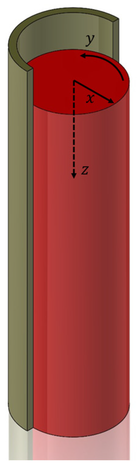
A hybrid coordinate system is constructed with the geometric center of the billet cross-section as the origin: the radial direction of the billet is defined as the r-axis; the direction from the center to the outer arc side is taken as the reference to set the initial direction (0°) of the θ-axis; the casting direction is designated as the z-axis, the hybrid coordinate system is shown in Figure 1 (drawn with SolidWorks 2023 SP5; Dassault Systèmes, Waltham, MA, USA).

2.2. Equal-Area Meshing of Round Billets

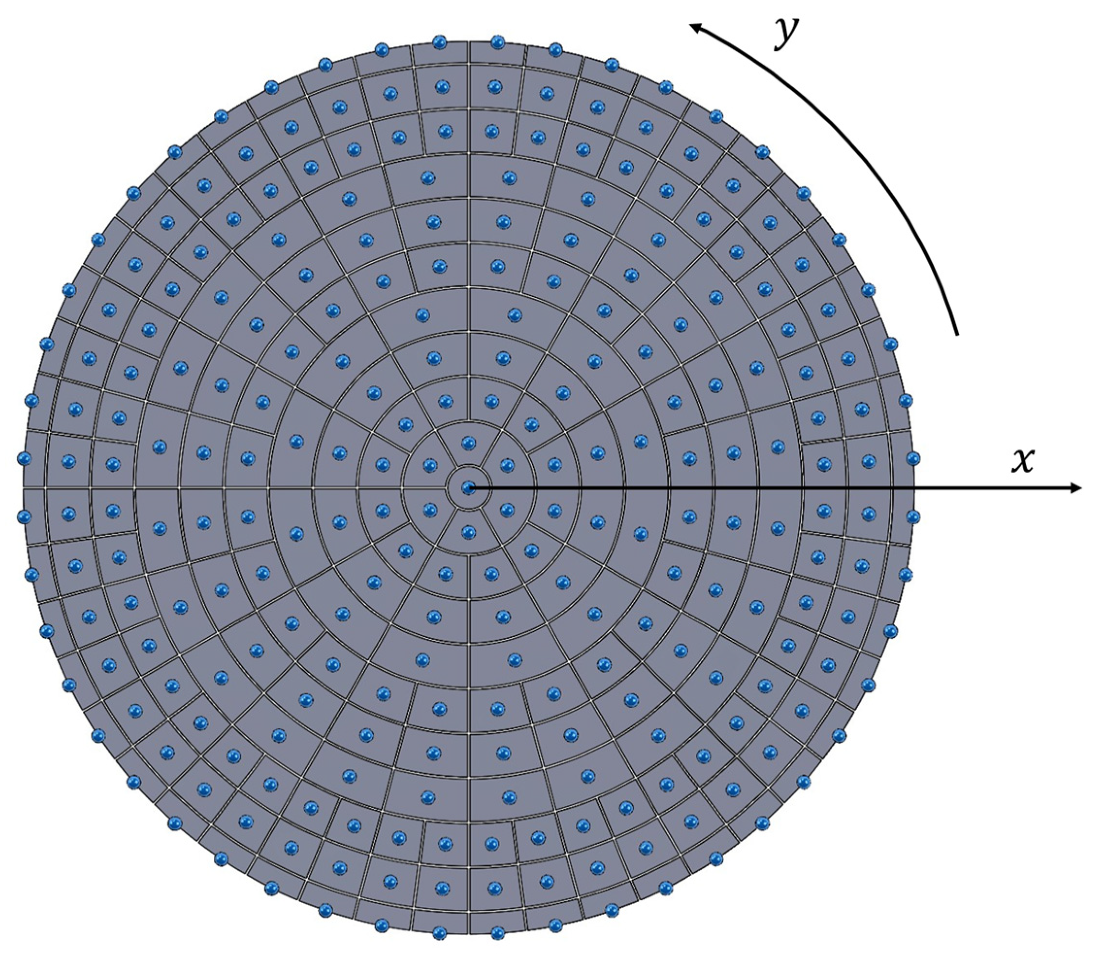
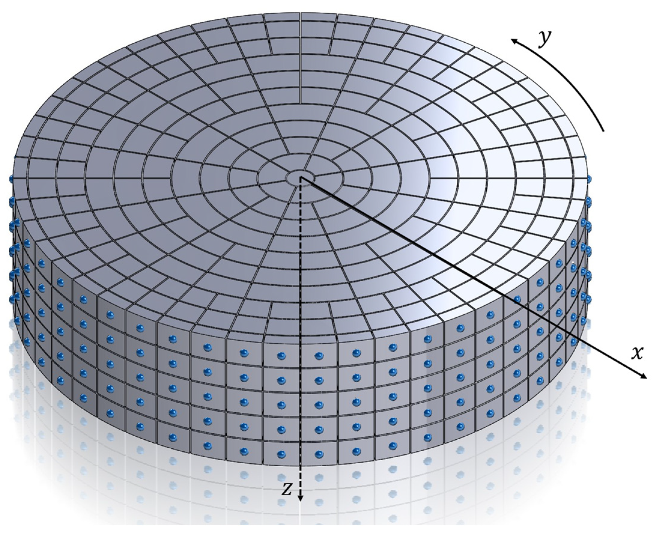
In view of the geometric characteristics of round billets and considering the complexity of boundary conditions, particularly the circumferential heat transfer inhomogeneity caused by the contact area between rolls and billets, this study performs three-dimensional mesh generation for the billet: the mesh at the center is circular, and the node coordinates of boundary meshes lie on the outer circle. The results of mesh generation are shown in Figure 2 and Figure 3.

Set the radial division number as Nx, the division number of the outermost circumference as Nr, and the mesh merging interval number as Nm. According to mesh characteristics, the Nx be an integer multiple of Nm, and Nr be an integer power of 2. Define the circumferential mesh number at radial position x as Ny[x], whose calculation formula is as Equation (1):

$$Ny[x]=\left\{\begin{array}{l}{\displaystyle \frac{Nr}{2^{\mathrm{int}(\frac{Nx-x}{Nm})}}} x>1\\ 1 x=1\end{array}\right.$$

(1)

where int () denotes the floor function that rounds down the value inside the parentheses. The spatial step sizes in the x, y, and z directions are denoted as Δx[x], Δy[x] and Δz, respectively.

When calculating the mesh spatial step size based on the equal-area method, a constant reference value of S for the mesh unit area is first determined: the mesh unit area corresponding to the central node and boundary nodes is S/2, while that corresponding to other internal nodes is S. The calculation formula for the reference value is given by Equation (2):

$$S={\displaystyle \frac{\pi R^2}{1+{\displaystyle \sum _{x=1}^{x=Nx-1}}Ny[x]+\frac{Ny[Nx - 1]}{2}}}$$

(2)

Based on the constant reference value of S, the calculation formulas for the spatial step sizes of each node are derived as shown in Equation (3):

$$\begin{gathered} \mathrm{\Delta }Ay[x]= \left\{\begin{array}{c}{\displaystyle \frac{2\pi }{Ny[x]}} x>1\\ 2\pi x=1\end{array}\right. \\ \mathrm{\Delta }x[x]=\left\{\begin{array}{c}{\displaystyle \frac{S}{2\mathrm{\Delta }Ay[x]}} x=Nx\\ \sqrt{{\displaystyle \frac{S}{\pi }}} x=0\\ {\displaystyle \frac{S}{\mathrm{\Delta }Ay[x]}} else\hfill \end{array}\right. \\ \mathrm{\Delta }y[x]= \left\{\begin{array}{c}{\displaystyle \frac{2\pi \mathrm{\Delta }x[x]}{Ny[x]}} x>1\\ 2\pi \mathrm{\Delta }x[x] x=1\end{array}\right. \end{gathered}$$

(3)

where ΔAy[x], Δx[x], Δy[x] denote the circumferential arc step size, radial step size, and circumferential step size of each mesh at coordinate x, respectively. Using the above parameters, the polar coordinates (Px[x, y, z], Py[x, y, z], Pz[x, y, z) of each node can be further calculated as shown in Equation (4):

$$\begin{gathered} Px[x,y,z]={\displaystyle \sum _{x=1}^{x=x}}\mathrm{\Delta }x[x] \\ Py[x,y,z]={\displaystyle \sum _{y=1}^{y=y}}\mathrm{\Delta }y[y] \\ Pz[x,y,z]=z\cdot \mathrm{\Delta }z \end{gathered}$$

(4)

To facilitate subsequent calculations, an equivalent step size ΔEx[x] is introduced, with its calculation formula shown in Equation (5):

$$\mathrm{\Delta }Ex[x]=\left\{\begin{array}{c}2\mathrm{\Delta }x[x] x=1,x=Nx\hfill \\ \mathrm{\Delta }x[x] else\hfill \end{array}\right.$$

(5)

2.3. State Variable Storage

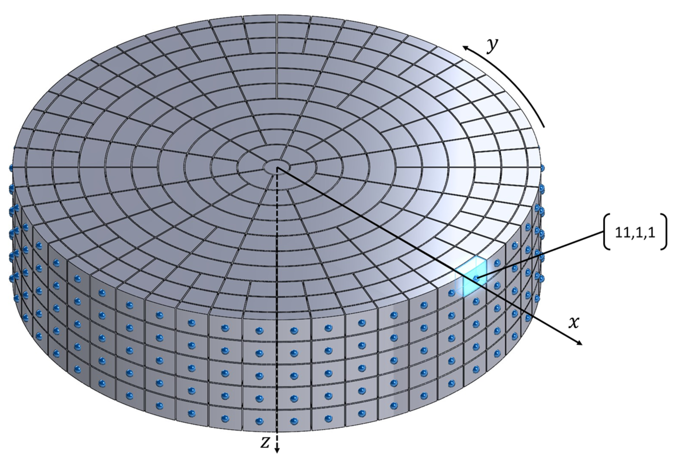
Nodes of the 3D hexahedral mesh for the billet are numbered in the format [x, y, z]. For instance, the position of node [11, 1, 1] is shown in Figure 4.

The cross-sectional area, volume, and mass of all meshes are stored in arrays Sg[x, y], V[x, y] and M[x, y], respectively, with the calculation formulas as shown in Equation (6):

$$\begin{gathered} Sg[x,y]=\mathrm{\Delta }x[x]\cdot \mathrm{\Delta }y[x] \\ V[x,y]=S[x,y]\cdot \mathrm{\Delta }z \\ M[x,y]=V[x,y]\cdot {\rho }_{T=20°\mathrm{C}} \end{gathered}$$

(6)

where ρ is the density of the billet material at 20 °C.

The boundary lengths of each mesh in the −x, +x, −y, and +y directions are stored in array L[x, y], calculated as shown in Equation (7):

$$L[x,y]=\left[\begin{array}{c}\left({\displaystyle \sum _{x=1}^{x=x}}\left(\mathrm{\Delta }x[x]\right)-{\displaystyle \frac{\mathrm{\Delta }x[x]}{2}}\right)\cdot \mathrm{\Delta }Ay[x],\hfill \\ \left({\displaystyle \sum _{x=1}^{x=x}}\left(\mathrm{\Delta }x[x]\right)+{\displaystyle \frac{\mathrm{\Delta }x[x]}{2}}\right)\cdot \mathrm{\Delta }Ay[x],\hfill \\ \mathrm{\Delta }x[x],\hfill \\ \mathrm{\Delta }x[x]\hfill \end{array}\right]$$

(7)

Based on the node numbering, the following storage structures are constructed:

• Number of surrounding nodes (Ns[x, y, z]): Stores the number of adjacent nodes around each node;
• Coordinates of surrounding nodes (G[x, y, z]): Stores the coordinates of adjacent nodes in the order of −x, +x, −y, +y, −z, +z;
• Connection lengths between nodes (W[x, y, z]): Stores the lengths of connections between the current node and its adjacent nodes;
• Shared mesh area (Sa[x, y, z]): Stores the equivalent spatial step sizes in the x, y, and z directions. The maximal shared mesh area occurs at the billet center, where both the radial step and the circumferential step reach their maximum values. For the φ600 mm billet, the maximal shared mesh area is calculated to be 0.028 m²;
• Equivalent spatial step sizes (E[x, y, z]): Stores the equivalent spatial step sizes in the x, y, and z directions;
• Boundary areas (B[x, y, z]): Stores the boundary areas of nodes in the x, y, and z directions.

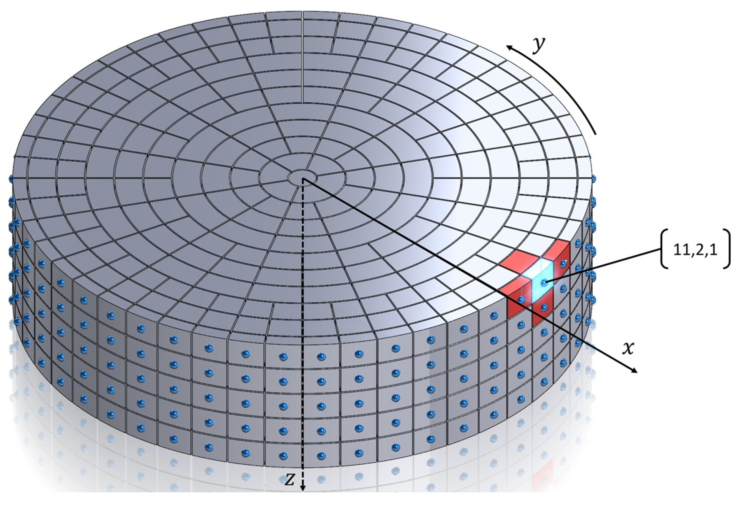
As shown in Figure 5, taking node [11, 2, 1] as an example, the Ns[x, y, z] for node [11, 2, 1] is given in Equation (8):

$$Ns[x,y,z{]}_{x=11,y=2,z=1}=4$$

(8)

The G[x, y, z] for node [11, 2, 1] is given in Equation (9):

$$G[x,y,z{]}_{x=11,y=2,z=1}=\left[\begin{array}{c}\left[x-1,y,z\right],\\ [x,y+1,z],\\ [x,y-1,z],\\ [x,y,z+1],\end{array}\right]$$

(9)

The W[x, y, z] for node [11, 2, 1] is given in Equation (10):

$$W[x,y,z{]}_{x=11,y=2,z=1}=\left[\begin{array}{c}{\displaystyle \frac{\mathrm{\Delta }Ex[x]+\mathrm{\Delta }Ex[x-1]}{2}},\hfill \\ \mathrm{\Delta }y[x],\hfill \\ \mathrm{\Delta }y[x],\hfill \\ \mathrm{\Delta }z\hfill \end{array}\right]$$

(10)

The Sa[x, y, z] for node [11, 2, 1] is given in Equation (11):

$$Sa[x,y,z{]}_{x=11,y=2,z=1}=\left[\begin{array}{c}L[x,y][1]\cdot \mathrm{\Delta }z[z],\hfill \\ \mathrm{\Delta }x[x]\cdot \mathrm{\Delta }z,\hfill \\ \mathrm{\Delta }x[x]\cdot \mathrm{\Delta }z,\hfill \\ Sg[x,y]\hfill \end{array}\right]$$

(11)

The E[x, y, z] for node [11, 2, 1] is given in Equation (12):

$$E[x,y,z{]}_{x=11,y=2,z=1}=\left[\begin{array}{c}[\mathrm{\Delta }Ex[x],\mathrm{\Delta }Ex[x-1]],\hfill \\ [\mathrm{\Delta }y[x],\mathrm{\Delta }y[x]],\hfill \\ [\mathrm{\Delta }y[x],\mathrm{\Delta }y[x]],\hfill \\ [\mathrm{\Delta }z,\mathrm{\Delta }z]\hfill \end{array}\right]$$

(12)

The B[x, y, z] for node [11, 2, 1] is given in Equation (13):

$$B[x,y,z{]}_{x=11,y=2,z=1}=\left[\begin{array}{c}\mathrm{\Delta }y[x]\cdot \mathrm{\Delta }z,\hfill \\ 0,\hfill \\ 0\hfill \end{array}\right]$$

(13)

3. Finite Difference Mathematical Calculation Model

The first law of thermodynamics, as the core of the principle of energy conservation, provides a physical basis for modeling the three-dimensional temperature field of continuous casting slabs. In the discretized analysis of the slab heat transfer process, a typical micro-element is selected as the control volume, and its energy conservation relationship can be expressed as: after a time step Δt, the internal energy of the micro-element is equal to its internal energy at the previous moment plus the energy entering the micro-element minus the energy flowing out of the micro-element.

In the model, the enthalpy of each node at time t is denoted as H[x, y, z][t], and the enthalpy after a time step of Δt is H[x, y, z][t + Δt]. The explicit finite-difference equation is expressed as Equation (14):

$$\begin{gathered} H[x,y,z][t+\mathrm{\Delta }t]=H[x,y,z][t]+{\displaystyle \frac{\mathrm{\Delta }t}{M[x,y,z]}}\cdot \\ \left(\begin{array}{c}{\displaystyle \sum _{i=1}^{i=Ns[x,y,z]}}\left(\begin{array}{c}Sa[x,y,z][i][t]\cdot \lambda [x,y,z][i][t]\cdot \\ {\displaystyle \frac{T[G[x,y,z][i]][t]-T[x,y,z][t]}{W[x,y,z][i][t]}}\end{array}\right)\hfill \\ -{\displaystyle \sum _{j=1}^{j=3}}\left(B[x,y,z][j][t]\cdot Q[x,y,z][j][t]\right)\hfill \end{array}\right) \end{gathered}$$

(14)

The corresponding convergence formula is shown in Equation (15)

$$\begin{gathered} \mathrm{\Delta }t\le {\displaystyle \frac{M[x,y,z]\cdot H[x,y,z][t]}{T[x,y,z][t]}}\cdot \\ {\displaystyle \frac{1}{\begin{array}{c}{\displaystyle \sum _{i=1}^{i=Ns[x,y,z]}}\left(\frac{Sa[x,y,z][i][t]\cdot \lambda [x,y,z][i][t]}{W[x,y,z][i][t]}\right)\hfill \\ +{\displaystyle \sum _{j=1}^{j=3}}\left(B[x,y,z][j][t]\cdot \frac{Q[x,y,z][i][t]}{T[x,y,z][t]-Tf}\right)\hfill \end{array}}} \end{gathered}$$

(15)

The meanings of variables in Equation (15) are shown in

Table 1. Meanings of variables in Equation (15).

Variable Symbol	Meaning	Unit
T[G[x, y, z][i]][t]	Temperature of the i-th surrounding node of node [x, y, z] at time t	°C
T[x, y, z][t]	Temperature of node [x, y, z] at time t	°C
W[x, y, z][i][t]	Connection length between node [x, y, z] and its i-th surrounding node at time t	m
B[x, y, z][j][t]	Boundary area of node [x, y, z] in the j-th coordinate axis direction at time t	m2
Q[x, y, z][j][t]	Boundary heat flux density of node [x, y, z] in the j-th coordinate axis direction at time t	W/m2
H[x, y, z][t + Δt]	Enthalpy of node [x, y, z] at time of t + Δt	J/kg
H[x, y, z][t]	Enthalpy of node [x, y, z] at time of t	J/kg
M[x, y, z]	Mass of node [x, y, z]	kg
Ns[x, y, z]	Number of surrounding nodes of node [x, y, z]	/
S[x, y, z][i][t]	Shared mesh area between node [x, y, z] and its i-th surrounding node at time t	m2
λ[x, y, z][i][t]	Comprehensive thermal conductivity between node [x, y, z] and its i-th surrounding node at time t	W/(m·°C)

:

When all time parameters t (except the enthalpy term) on the right-hand side of Equation (7) are changed to t + Δt, the equation becomes the implicit Equation (16):

$$\begin{gathered} H[x,y,z][t+\mathrm{\Delta }t]=H[x,y,z][t]+{\displaystyle \frac{\mathrm{\Delta }t}{M[x,y,z]}}\cdot \\ \left(\begin{array}{c}{\displaystyle \sum _{i=1}^{i=Ns[x,y,z]}}\left(\begin{array}{c}Sa[x,y,z][i][t+\mathrm{\Delta }t]\cdot \lambda [x,y,z][i][t+\mathrm{\Delta }t]\cdot \\ {\displaystyle \frac{T[G[x,y,z][i]][t+\mathrm{\Delta }t]-T[x,y,z][t+\mathrm{\Delta }t]}{W[x,y,z][i][t+\mathrm{\Delta }t]}}\end{array}\right)\hfill \\ -{\displaystyle \sum _{j=1}^{j=3}}\left(B[x,y,z][j][t+\mathrm{\Delta }t]\cdot Q[x,y,z][j][t+\mathrm{\Delta }t]\right)\hfill \end{array}\right) \end{gathered}$$

(16)

When all time-dependent variables (excluding the enthalpy term) on the right-hand side of Equation (7) are replaced with their average values over the time step Δt, the equation takes a semi-implicit form. Assuming these variables vary linearly within Δt, the semi-implicit equation is shown in Equation (17).

$$\begin{gathered} H[x,y,z][t+\mathrm{\Delta }t]=H[x,y,z][t]+{\displaystyle \frac{\mathrm{\Delta }t}{4\cdot M[x,y,z]}}\cdot \\ \left(\begin{array}{c}{\displaystyle \sum _{i=1}^{i=Ns[x,y,z]}}\left(\begin{array}{c}\left(Sa[x,y,z][i][t]+Sa[x,y,z][i][t+\mathrm{\Delta }t]\right)\cdot \hfill \\ \left(\lambda [x,y,z][i][t]+\lambda [x,y,z][i][t+\mathrm{\Delta }t]\right)\cdot \hfill \\ {\displaystyle \frac{\left(\begin{array}{c}T[G[x,y,z][i]][t]\hfill \\ +T[G[x,y,z][i]][t+\mathrm{\Delta }t]\hfill \\ -T[x,y,z][t]-T[x,y,z][t+\mathrm{\Delta }t]\hfill \end{array}\right)}{W[x,y,z][i][t]+W[x,y,z][i][t+\mathrm{\Delta }t]}}\hfill \end{array}\right)\hfill \\ -{\displaystyle \sum _{j=1}^{j=3}}\left(\begin{array}{c}\left(B[x,y,z][j][t]+B[x,y,z][j][t+\mathrm{\Delta }t]\right)\hfill \\ \cdot \left(Q[x,y,z][j][t]+Q[x,y,z][j][t+\mathrm{\Delta }t]\right)\hfill \end{array}\right)\hfill \end{array}\right) \end{gathered}$$

(17)

The calculation formula for λ[x, y, z][i][t] in Equation (17) is shown in Equation (18).

$$\lambda [x,y,z][i][t]=\left\{\begin{array}{c}{\displaystyle \frac{\lambda a+\lambda b}{2}} \left(x=G\left[x,y,z\right]\left[i\right]\left[1\right]\right)\&\left(x\ne 1\right)\&\left(G[x,y,z][i][1]\ne 1\right) \hfill \\ {\displaystyle \frac{\lambda a+\lambda b}{2}} \left(z\ne G[x,y,z][i][3]\right) \hfill \\ {\displaystyle \frac{\lambda a\cdot \lambda b\cdot Ln\left(\frac{Px[x,y,z]}{Px[G[x,y,z][i]]}\right)}{\lambda a\cdot Ln\left(\frac{Px[x,y,z] - \frac{\mathrm{\Delta }Ex[x,y,z]}{2}}{Px[G[x,y,z][i]]}\right)+\lambda b\cdot Ln\left(\frac{Px[x,y,z]}{Px[x,y,z] - \frac{\mathrm{\Delta }Ex[x,y,z]}{2}}\right)}} \hfill \\ \left(x\ne G[x,y,z][i][1]\right)\&\left(x\ne 1\right)\&\left(G[x,y,z][i][1]\ne 1\right)\hfill \\ \lambda a \left(x\ne G[x,y,z][i][1]\right)\&\left(x=1\right)\hfill \\ \lambda b \left(x\ne G[x,y,z][i][1]\right)\&\left(G[x,y,z][i][1]=1\right)\hfill \end{array}\right.$$

(18)

where λ_a and λ_b correspond to the thermal conductivities associated with the temperatures of the central node and the surrounding node, respectively.

Based on the theory of numerical computation methods, a comparative analysis of the characteristics of explicit, implicit, and semi-implicit schemes in terms of computational efficiency, numerical accuracy, and solution strategies reveals the following:

(1)

The explicit scheme directly calculates the current temperature distribution using the temperature field at the previous moment without the need for iterative solving, thus achieving the optimal computational efficiency. The time step for the explicit scheme must satisfy the stability condition, which requires the time step to be smaller than the critical value determined by the grid size and thermal diffusivity. For the finest mesh in this model, the minimum radial step is 0.5 mm, and the thermal diffusivity of typical steel is approximately 5 × 10⁻⁶ m²/s. The resulting critical time step is approximately 0.005 s. Therefore, the explicit scheme in this study uses a time step of 0.005 s. The stable time step range is from 0.002 to 0.005 s, depending on the local grid size, but a uniform time step of 0.005 s is applied across the entire computational domain to ensure stability.

(2)

The explicit scheme is constrained by stability conditions and thus requires a small time step, which in turn leads to significant accumulation of computational errors. For the present model, the required small time step is in the range of 0.002 to 0.005 s, with a uniform value of 0.005 s applied throughout the computational domain. This restriction is necessary to ensure numerical stability, given the smallest grid spacing of 0.5 mm and the thermal diffusivity of steel.

(3)

The explicit scheme directly solves the temperature field evolution equation using the explicit difference method. For the algebraic equations formed by the implicit and semi-implicit schemes, an improved Gauss–Seidel iterative algorithm is adopted for solution. Specifically, a chase method (Thomas algorithm) solution framework is established for the −x and −y directions, respectively, and the iterative accuracy is controlled by setting a convergence threshold. Compared with the explicit difference method, the implicit and semi-implicit schemes achieve higher computational efficiency in multi-dimensional temperature field calculations.

Considering that 3D temperature field calculation in practical applications needs to balance the differentiated requirements of dynamic response speed and result accuracy, its calculation modes can be divided into two categories: online calculation and offline calculation. Online calculation mainly targets scenarios that require real-time feedback on the dynamic evolution of physical fields, with real-time performance as the primary constraint. Given that the explicit scheme has the inherent attribute of a non-iterative solution, its computational efficiency is optimal among the three schemes and can meet the requirement of rapid response to the dynamic evolution of temperature fields; thus, adopting the explicit scheme is more efficient. Offline calculation focuses on in-depth analysis of the evolution laws of temperature fields and high-precision simulation. The semi-implicit scheme can achieve the optimization of comprehensive accuracy on the premise of ensuring computational stability by introducing time-averaged data within the time step, which can fully adapt to the technical requirements of high-precision analysis.

4. Boundary Conditions of Solidification Heat Transfer Model

4.1. Calculation of Mold Boundary Conditions

The variation in the surface temperature of the slab in the mold is relatively complex. It is generally accepted that the heat flux at the slab boundary is related to the casting speed and the distance from the meniscus. The heat flux adopted in this paper is shown in Equation (19).

$$q_m=ef·2·v^{0.56}·e^{-1.5L}\times {10}^6$$

(19)

where q_m represents the heat flux at varying positions of the mold (W/m²), v denotes the casting speed (m/min), l signifies the distance from the meniscus (m), e is the base of the natural logarithm, and ef is the correction coefficient for this equation. The correction coefficient ef in Equation (19) was calibrated using on-site measurements of the mold cooling water. The total heat extracted by the mold was calculated from the cooling water flow rate and the inlet–outlet temperature difference. The ef values for different billet cross-sections were then obtained by least-squares fitting using Equation (19) under various casting speeds and cross-sections. The calibrated ef values are listed in

Table 2. The corrected ef coefficient.

Cross-Sectional Diameter (mm)	The Value of Ef Coefficient
180	0.896
200	0.8556
240	0.9577
250	0.9577
300	0.9967
350	0.9959
400	1.0589
450	1.064
500	1.12967
600	1.3181

. This calibration process is essentially a semi-empirical approach based on industrial data. A sensitivity analysis was performed to evaluate the impact of ef on the predicted temperature. Taking the φ600 mm billet and a casting speed of 0.24 m/min as the baseline, the ef value was perturbed by ±10%. The resulting change in the surface temperature at the straightening zone was approximately ±8.2 °C. This moderate sensitivity indicates that accurate calibration of ef is important for precise temperature prediction.

4.2. Calculation of Boundary Conditions of the Secondary Cooling Zone

In the secondary cooling zone, the heat transfer of the slab is primarily accomplished through spray convective heat transfer, surface radiative heat transfer of the slab, contact conduction heat transfer between the slab and roll system, and accumulated heat transfer via the liquid film formed by cooling water on the slab surface. Owing to the specific geometric characteristics of the round slab, such as the axisymmetry of the cross-section and the absence of corners and combined with the structural features of the roll system, the accumulated heat transfer effect of cooling water on the slab surface is generally negligible. The axisymmetry allows the three-dimensional temperature field to be simplified into a two-dimensional axisymmetric problem. The absence of corners means that the round billet does not suffer from the corner supercooling or corner crack problems commonly seen in billets or slabs.

Spray heat transfer dominates in the first several cooling zones, and the quantitative characterization of its heat transfer coefficient needs to correlate the coupling relationship between water flow density and slab surface temperature. In this paper, differentiated heat transfer coefficient calculation models are adopted for different cooling zones, among which the specific expression for the first secondary cooling zone is shown in Equation (20):

$$hf=\left\{\begin{array}{c}1.9\times {10}^9\times T{w}^{-2.295}\times W^{0.659} Tw>900 ℃\\ 3.01\times {10}^6\times T{w}^{-1.491}\times W^{0.7749} Tw\le 900 ℃\end{array}\right.$$

(20)

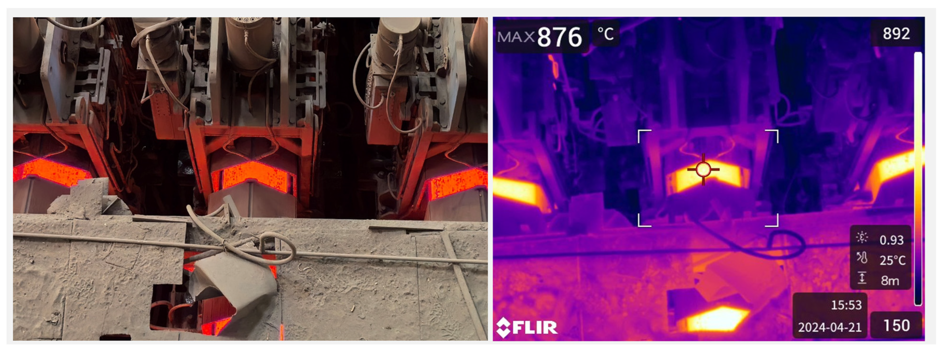
where hf is the heat transfer coefficient between the slab and spray water (W/(m⁻²·°C)), Tw is the surface temperature of the slab (°C), and W is the water flow density (kg/(m²·s)). The coefficients in Equation (20) are derived from standard forms in the literature. For practical application to this specific caster, local calibration was performed according to the nozzle arrangement, water flow density distribution, and billet surface temperature measurements (as shown in Figure 6). A one-dimensional inverse heat transfer method was used to adjust the water flow density multipliers for each cooling zone. The calibration achieved a temperature deviation between the model predictions and the measured values within ±10 °C.

A sensitivity analysis was carried out to evaluate the effect of the spray cooling parameters on the predicted temperature. Based on the φ600 mm billet and a casting speed of 0.24 m/min, the water flow density in the secondary cooling zone was perturbed by ±10%. The resulting change in the surface temperature at the straightening zone was approximately ±12.5 °C. This indicates that the model is most sensitive to the water flow density in the secondary cooling zone, which is consistent with physical understanding.

The contact heat transfer between the slab and rolls is calculated by Equation (21):

$$qs=1151.3\times T{w}^{0.76}\times v^{-0.2}\times {\left(2\alpha \right)}^{-0.17}$$

(21)

where qs is the heat flux at the contact interface between the slab and rolls (W/m²), v is the casting speed (m/min), and 2α is the angle corresponding to the arc length of the contact portion between the rolls and the slab (°).

The radiant heat transfer of the slab is calculated as shown in Equation (22):

$$qr=\epsilon \sigma \left({\left(Ts+273\right)}^4+{\left(Tf+273\right)}^4\right)$$

(22)

where qr is the heat flux of the slab’s radiant heat transfer (W/m²), ε is the emissivity, σ is the Boltzmann constant (5.67 × 10⁻⁸ W/(m²·K⁴)), Ts is the surface temperature of the slab (°C), and Tf is the air temperature in the secondary cooling chamber (°C).

5. Development of Calculation Software for Round Billet Solidification Heat Transfer Model

5.1. Development Environment and Optimization Strategies

To address the high-performance computing requirements of numerical simulations in continuous casting processes, the system must overcome critical challenges such as secure memory management, efficient data access, and real-time heat conduction calculations. Leveraging C++ as the development language, the system translates algorithmic logic into highly optimized machine code through zero-cost abstractions, while RAII resource management paradigms and STL smart pointer systems establish deterministic memory deallocation mechanisms to ensure resource safety during large-scale parallel computations. At the data access level, cache-like technologies reduce disk I/O overhead to improve data retrieval efficiency, while hash tables and other data mapping structures enable 0 (1) time complexity key-value lookups. Combined with write-back cache update strategies, these ensure data consistency in multithreaded environments. The heat conduction calculation module employs a dynamic threshold-based discrimination mechanism to automatically skip redundant computations when temperature gradients fall below critical values. Simultaneously, SIMD instruction set integration accelerates floating-point operations through vectorization, reducing computational workload by 35% and significantly enhancing the execution efficiency of core algorithms. All performance tests were performed on the same workstation: Intel Core i7-14700K CPU @ 3.80 GHz, 16 GB RAM, Windows 10, single-thread execution. The code was compiled with Microsoft Visual Studio 2019 using the/O₂ optimization flag. For the test case (φ600 mm, 42CrMo, 0.24 m/min, simulation length 15 m), the wall-clock times are as follows: the baseline code (no SIMD, no threshold optimization) ran in 40.0 min; with SIMD only, the time was reduced to 28.9 min; with both SIMD and temperature gradient threshold optimization (5 °C/mm), the time was further reduced to 26.4 min. Relative to the baseline, the total improvement is approximately 35%.

This multi-dimensional technical integration enables the system to meet industrial-grade real-time simulation requirements while maintaining the accuracy of physical models. This multi-dimensional technical integration enables the system to meet industrial-grade real-time simulation requirements while maintaining the accuracy of physical models.

5.2. Calculation Example of Solidification Heat Transfer Model

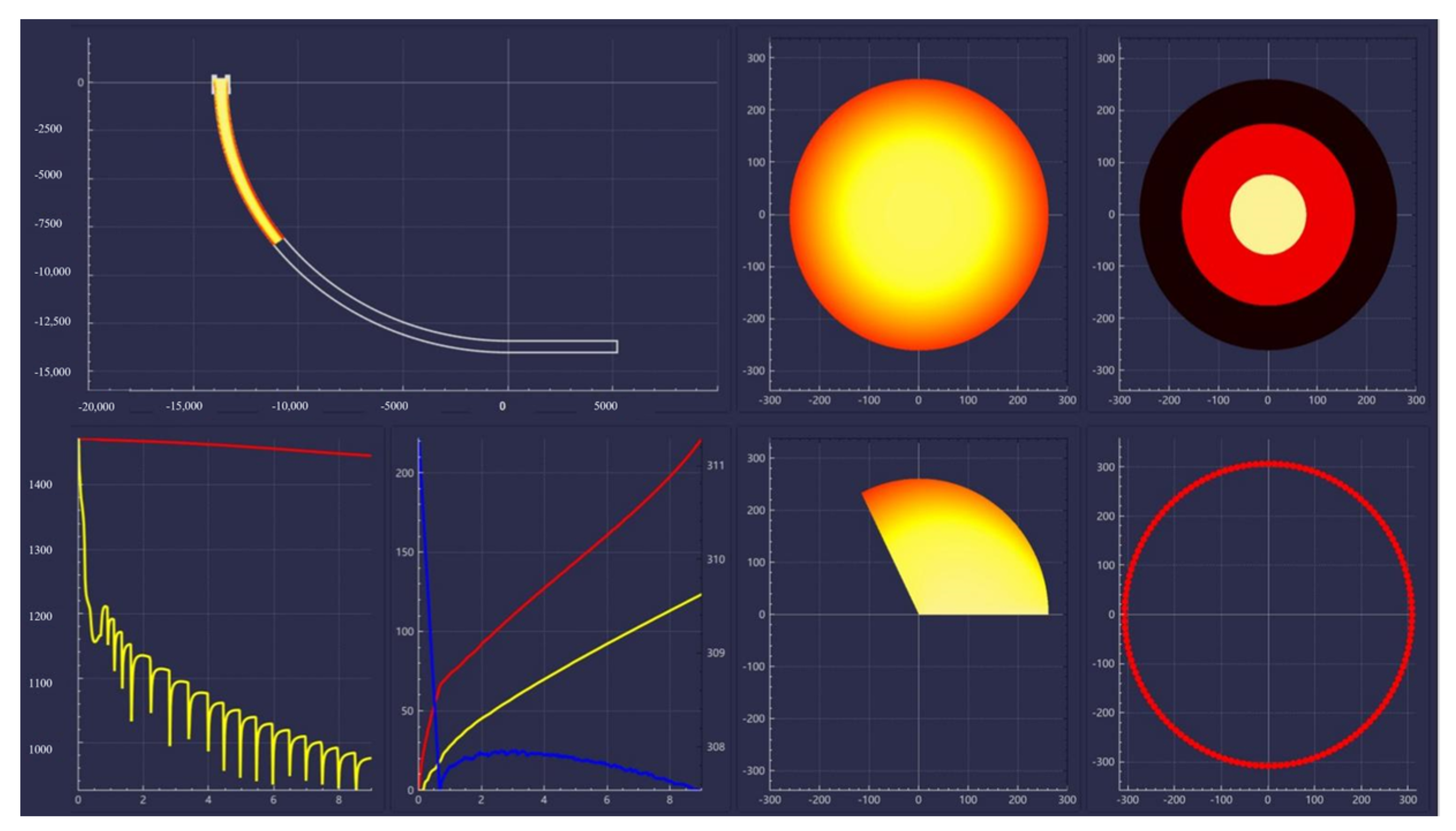
Based on a continuous caster, which produces castings with a cross-section of φ600 mm at a casting speed of 0.24 m/min for the 42CrMo steel grade, the software calculation interface is shown in Figure 7.

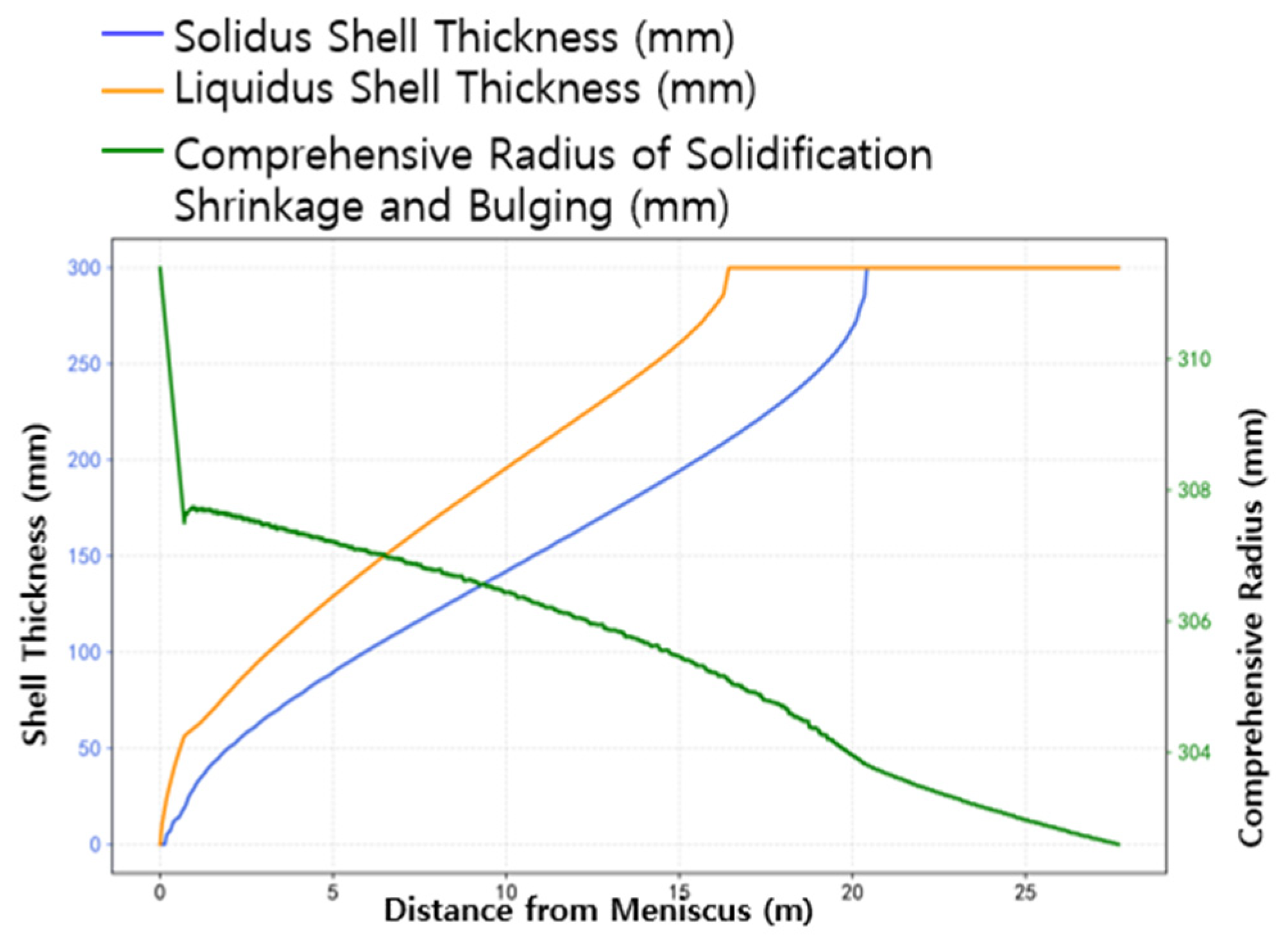
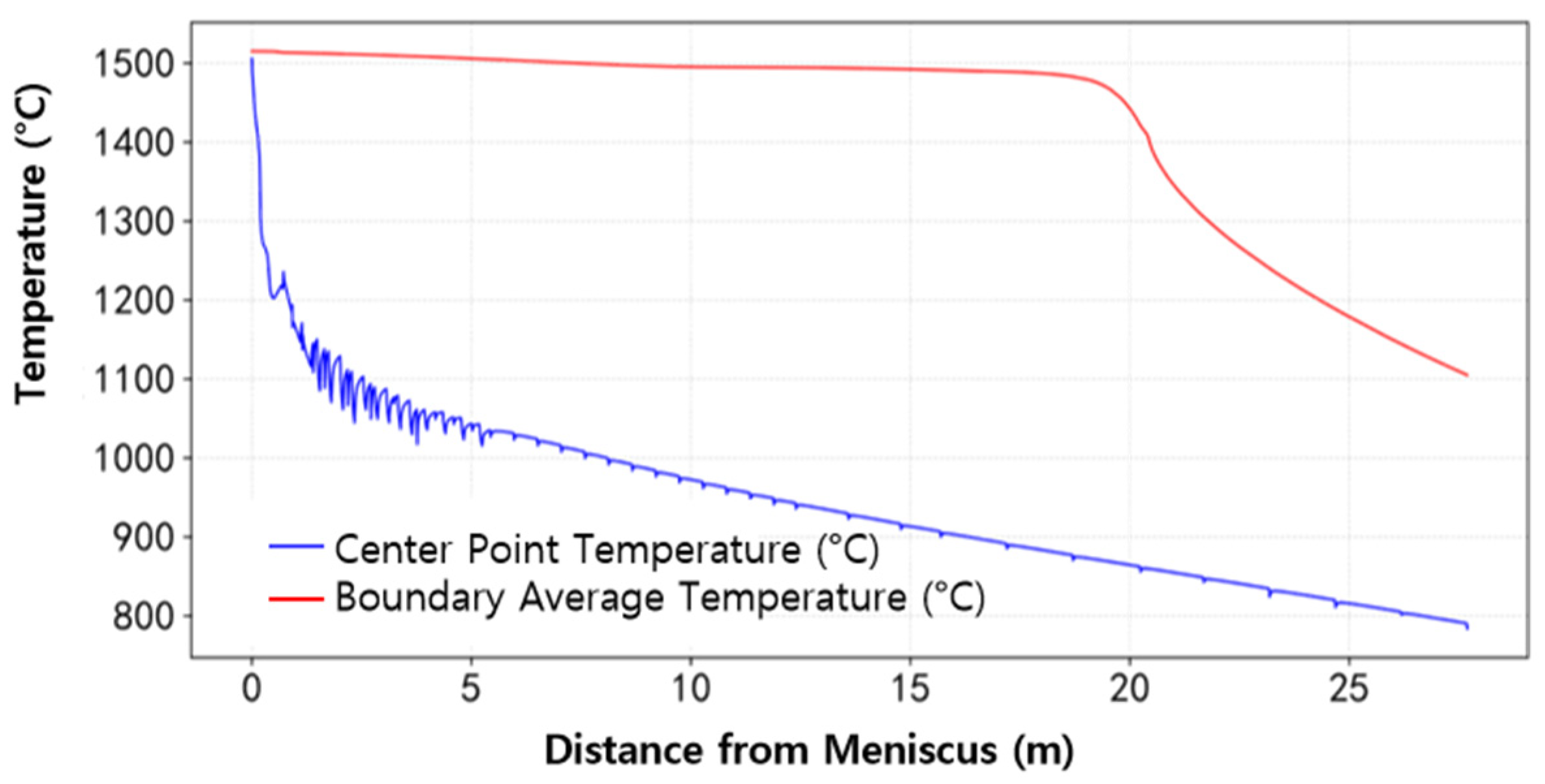
The calculated temperature variation curves of different key points are presented in Figure 8, and the shell growth curve along the thickness direction is shown in Figure 9.

5.3. Industrial Validation

On-site monitoring was carried out for the production process of the round billet continuous caster corresponding to the calculation case. The surface temperature of the cast billet was measured in front of the straightening zone, and the results are presented in Figure 6.

Field measurement results show that the average temperature of the slab before straightening is 876 °C. The calculated value of this model for the same process node is 887 °C, as shown in Figure 6. Error analysis indicates that the absolute deviation between the model-calculated value and the measured value is 11 °C, and the relative deviation is 1.25%. Both indicators fall within the allowable engineering error range, verifying the accuracy of the model in temperature field prediction. In this validation case using 42CrMo steel, the billet surface temperature ranges from 850 to 1150 °C and the liquid core temperature ranges from 1490 to 1520 °C. Both of these ranges fall within the model’s applicable temperature range of 800–1520 °C, confirming that the validation conditions are appropriate for assessing the model’s performance.

On-site measurements of the slab diameter were conducted using a batch-based, multi-time data collection method; the results are presented in

Table 3. Round billet diameter measurement data.

Number	Diameter (Non-Flat Region)	Diameter (Flat Region)	Diameter (Average)
1	601	598	599.5
2	602	598	600
3	601	598	599.5
4	601	598	599.5
5	601	598	599.5
6	601	598	599.5
7	602	599	600.5
8	601.5	598	599.75
9	601	598	599.5
10	601	598	599.5
11	601	597	599
12	601.5	598	599.75
13	600.5	597	598.75
14	600.5	598	599.25
15	601.5	598	599.75
16	601	597	599
17	600.5	598	599.25
18	601	597	599
19	600.5	598	599.25
20	601	598	599.5
21	600.5	598	599.25
22	601	599	600
23	600.5	598	599.25
24	601.5	599	600.25
Average value of measured data		599.5

.

The measured average diameter of the cast billet is 599.5 mm, while the final diameter of the cold-state cast billet calculated by this model is 597.548 mm. Using the measured value as the reference, the relative error of the calculation result is 0.325%, which meets the engineering error requirement of 0.6%.

It should be noted that the current validation is based on a single caster configuration (billet diameter φ600 mm, steel grade 42CrMo, casting speed 0.24 m/min). The model calibration, especially the empirical correction factor ef in the mold heat flux model and the spray heat transfer coefficients in the secondary cooling zone, was performed specifically for this caster using on-site measurements of cooling water flow rate and temperature difference. Therefore, the model in its present form is locally calibrated and may not be directly transferable to other casters, billet sizes, steel grades, or operating conditions without recalibration. When applying the model to different production environments, users should redetermine the empirical coefficients (e.g., ef in Table 2, the spray correlation parameters in Equation (20)). Nevertheless, the overall modeling framework—including the hybrid coordinate system, equal-area meshing, and the explicit/semi-implicit finite-difference solver—is general and can be readily adapted to other configurations by replacing the boundary condition correlations and thermophysical properties. In the future, as more industrial data becomes available, we will extend the validation to additional casting speeds and steel grades.

5.4. Model Limitations and Future Work

The core physical basis of the current model is the heat conduction equation considering the latent heat of phase change. It does not yet couple complex physical effects such as fluid flow, stress evolution, air-gap formation, or solute segregation. The focus of this study is to construct an efficient three-dimensional temperature field model for industrial real-time applications, and therefore, a reasonable simplification of the physical processes has been made. Specifically, the model has the following limitations:

(i)

The model does not couple fluid flow in the liquid pool, so convective heat transfer and its effects on temperature distribution and macrosegregation cannot be simulated.

(ii)

The model does not consider thermal stress or mechanical stress, which are closely related to crack formation.

(iii)

The model does not consider air-gap formation between the billet and the mold or rolls, which would significantly alter the heat transfer boundary conditions.

(iv)

The model adopts an axisymmetric assumption for the billet cross-section, which neglects circumferential non-uniform heat transfer phenomena such as local cooling differences caused by roll contact. In addition, the model does not consider solute segregation during solidification.

In future work, we plan to extend the model in the following three directions. First, we will couple a thermomechanical solver for stress analysis to predict stress-related defects such as cracks. Second, we will introduce a two-phase flow model for the liquid region to simulate fluid flow and its effects on the temperature field and macrosegregation. Third, we will incorporate a micro-segregation model to describe the redistribution of solutes during solidification. These extensions will enable a more comprehensive simulation of the continuous casting process and provide better guidance for defect prevention.

6. Conclusions

This study constructed a 3D temperature field numerical calculation model for round billet continuous casting, which accurately characterizes geometric features via a hybrid coordinate system (radial r, circumferential θ, axial z) and an innovative mesh division strategy (central circular mesh and boundary equal-area discretization), and establishes a heat conduction solution system based on explicit/semi-implicit finite difference methods. Breaking through the limitations of traditional empirical methods, such as the square-root law for shell growth and the assumption of constant heat transfer coefficients in each cooling zone, the model realizes digital reconstruction of the slab solidification process and can provide theoretical support for dynamic water distribution optimization and process development of special steel grades when combined with intelligent manufacturing technologies in the future. The conclusions are as follows:

(1)

The spatial step size is set by the equal-area method, and the 3D mesh data structure is optimized to improve computational stability; the explicit finite difference method is adapted to efficient online calculation, the semi-implicit finite difference method meets high-precision offline analysis, and the computational load is reduced by 35% by combining SIMD instruction parallelization and a dynamic calculation strategy of temperature difference threshold.

(2)

The mold heat flux model achieves adaptive matching of different cross-sections through the correction coefficient ef, and the secondary cooling zone comprehensively couples multiple physical field effects such as spray heat transfer, roller contact heat conduction, and radiation heat transfer.

(3)

In the simulation results for 42CrMo steel with φ600 mm cross-section (casting speed 0.24 m/min), the deviation between the calculated surface temperature (887 °C) and the measured value (876 °C) in the straightening zone is 11 °C, the relative error between the calculated cold-state slab diameter (597.548 mm) and the measured average value (599.5 mm) is 0.325%, and the temperature field distribution and shell growth curve can accurately reflect the solidification law.

References

1. Guo, J.; Hong, X. Numerical solution of heat tranfer problem with flow and solidification in round billet continuous casting of steel. Commun. Nonlinear Sci. Numer. Simul. 1999, 4, 236–239. [Google Scholar] [CrossRef]
2. Sun, T.; Yue, F.; Wu, H.-J.; Guo, C.; Li, Y.; Ma, Z.-C. Solidification Structure of Continuous Casting Large Round Billets under Mold Electromagnetic Stirring. J. Iron Steel Res. Int. 2016, 23, 329–337. [Google Scholar] [CrossRef]
3. Yao, C.; Wang, M.; Zhang, M.; Xing, L.; Zhang, H.; Bao, Y. Effects of mold electromagnetic stirring on heat transfer, species transfer and solidification characteristics of continuous casting round billet. J. Mater. Res. Technol. 2022, 19, 1766–1776. [Google Scholar] [CrossRef]
4. Pourfathi, A.; Tavakoli, R. Thermal optimization of secondary cooling systems in the continuous steel casting process. Int. J. Therm. Sci. 2023, 183, 107860. [Google Scholar] [CrossRef]
5. Zhang, J.; Chen, D.-F.; Zhang, C.-Q.; Wang, S.-G.; Hwang, W.-S.; Han, M.-R. Effects of an even secondary cooling mode on the temperature and stress fields of round billet continuous casting steel. J. Mater. Process. Technol. 2015, 222, 315–326. [Google Scholar] [CrossRef]
6. Brezina, M.; Mauder, T.; Klimes, L.; Stetina, J. Comparison of Optimization-Regulation Algorithms for Secondary Cooling in Continuous Steel Casting. Metals 2021, 11, 237. [Google Scholar] [CrossRef]
7. Ai, S.; Long, M.; Yang, X.; Chen, D.; Duan, H. Prediction model for crack sensitive temperature region and phase fractions of slab under continuous casting cooling rates based on finite number of experiments. J. Mater. Res. Technol. 2023, 22, 1103–1117. [Google Scholar] [CrossRef]
8. Klimeš, L.; Březina, M.; Mauder, T.; Charvát, P.; Klemeš, J.J.; Štětina, J. Dry cooling as a way toward minimisation of water consumption in the steel industry: A case study for continuous steel casting. J. Clean. Prod. 2020, 275, 123109. [Google Scholar] [CrossRef]
9. Sarkar, J.; Modak, P.; Singh, S.B.; Chakrabarti, D. Effect of cooling-rate during solidification on the structure-property relationship of hot deformed low-carbon steel. Mater. Chem. Phys. 2021, 257, 123826. [Google Scholar] [CrossRef]
10. Zhang, Z.; Wu, M.; Zhang, H.; Hahn, S.; Wimmer, F.; Ludwig, A.; Kharicha, A. Modeling of the as-cast structure and macrosegregation in the continuous casting of a steel billet: Effect of M-EMS. J. Mater. Process. Technol. 2022, 301, 117434. [Google Scholar] [CrossRef]
11. Zhong, H.; Wang, R.; Han, Q.; Fang, M.; Yuan, H.; Song, L.; Xie, X.; Zhai, Q. Solidification structure and central segregation of 6Cr13Mo stainless steel under simulated continuous casting conditions. J. Mater. Res. Technol. 2022, 20, 3408–3419. [Google Scholar] [CrossRef]
12. Bratu, V.; Mortici, C.; Oros, C.; Ghiban, N. Mathematical model of solidification process in steel continuous casting taking into account the convective heat transfer at liquid–solid interface. Comput. Mater. Sci. 2014, 94, 2–7. [Google Scholar] [CrossRef]
13. Yang, Y.; Sun, J.; Liu, X.; Wang, W. Heat transfer behavior and formation mechanism of stainless steel cladding carbon steel plate during horizontal continuous liquid-solid composite casting. Int. Commun. Heat Mass Transf. 2024, 159, 108105. [Google Scholar] [CrossRef]
14. Li, D.-W.; Su, Z.-J.; Marukawa, K.; He, J.-C. Simulation on Effect of Divergent Angle of Submerged Entry Nozzle on Flow and Temperature Fields in Round Billet Mold in Electromagnetic Swirling Continuous Casting Process. J. Iron Steel Res. Int. 2014, 21, 159–165. [Google Scholar] [CrossRef]
15. Yin, H.; Yao, M. Inverse problem-based analysis on non-uniform profiles of thermal resistance between strand and mould for continuous round billets casting. J. Mater. Process. Technol. 2007, 183, 49–56. [Google Scholar] [CrossRef]
16. Yan, C.; Wang, F.; Mo, W.; Xiao, P.; Zhang, Q. Migration Behavior of Inclusions at the Solidification Front in Oxide Metallurgy. Materials 2023, 16, 4486. [Google Scholar] [CrossRef] [PubMed]
17. Bai, L.; Wang, B.; Zhong, H.; Ni, J.; Zhai, Q.; Zhang, J. Experimental and Numerical Simulations of the Solidification Process in Continuous Casting of Slab. Metals 2016, 6, 53. [Google Scholar] [CrossRef]
18. Zhang, P.; Wang, M.; Shi, P.; Xu, L. Effects of Alloying Elements on Solidification Structures and Macrosegregation in Slabs. Metals 2022, 12, 1826. [Google Scholar] [CrossRef]
19. Sanati, S.; Nabavi, S.F.; Farshidianfar, A. Laser wobble welding modeling process: A comprehensive review of fundamentals, methods, heating, and solidification modes. J. Manuf. Process. 2024, 131, 1703–1739. [Google Scholar] [CrossRef]
20. You, F.; Zhao, X.; Yue, Q.; Gu, Y.; Wang, J.; Bei, H.; Zhang, Z. A review on solidification of alloys under hypergravity. Prog. Nat. Sci. Mater. Int. 2023, 33, 279–294. [Google Scholar] [CrossRef]
21. Man, T.; Dai, Y.; Yao, J.; Xu, L.; Li, P.; Zhao, M.; Liu, Y.; Zhao, H. Segregation and carbide evolution in AISI D2 tool steel produced by curved continuous casting. J. Mater. Res. Technol. 2023, 26, 8254–8262. [Google Scholar] [CrossRef]
22. Yao, Y.; Liu, Z.; Li, B.; Xiao, L.; Gan, Y. Effect of steel strip feeding on the columnar-equiaxed solidification in a large continuous casting round bloom. J. Mater. Res. Technol. 2022, 20, 1770–1785. [Google Scholar] [CrossRef]
23. Zhang, Z.; Ji, C.; Ju, J.; Li, K.; Zhu, M. Micromechanical behavior and microcrack evolution in continuous casting slab: Experimental characterization, multiscale simulation and industrial validation. J. Mater. Process. Technol. 2025, 340, 118866. [Google Scholar] [CrossRef]
24. Guan, L.; Wang, Y.; Tan, X.; Liu, C.; Gui, W. Machine scheduling optimization via multi-strategy information-aware genetic algorithm in steelmaking continuous casting industrial process. Control. Eng. Pract. 2025, 164, 106404. [Google Scholar] [CrossRef]
25. Wang, B.; Ji, Z.-P.; Liu, W.-H.; Ma, J.-C.; Xie, Z. Application of Hot Strength and Ductility Test to Optimization of Secondary Cooling System in Billet Continuous Casting Process. J. Iron Steel Res. Int. 2008, 15, 16–20. [Google Scholar] [CrossRef]
26. Wang, X.; Wang, Z.; Liu, Y.; Du, F.; Yao, M.; Zhang, X. A particle swarm approach for optimization of secondary cooling process in slab continuous casting. Int. J. Heat Mass Transf. 2016, 93, 250–256. [Google Scholar] [CrossRef]
27. Wang, Y.-Z.; Zheng, Z.; Zhang, S.-Y.; Gao, X.-Q. A robust optimization method for multi-cast batching plans and casting start time dynamic decision in continuous casting process. Comput. Ind. Eng. 2024, 197, 110587. [Google Scholar] [CrossRef]
28. Li, J.; Nian, Y.; Liu, X.; Zong, Y.; Tang, X.; Zhang, C.; Zhang, L. Application of electromagnetic metallurgy in continuous casting: A review. Prog. Nat. Sci. Mater. Int. 2024, 34, 1–11. [Google Scholar] [CrossRef]
29. Li, T.; Li, H.; Li, R.; Wang, Z.; Wang, G. Analysis of ductile fractures at the surface of continuous casting steel during hot-core heavy reduction rolling. J. Mater. Process. Technol. 2020, 283, 116713. [Google Scholar] [CrossRef]
Figure 1. Schematic diagram of mathematical calculation model coordinate system for three-dimensional temperature field of round billet.
Metals 16 00579 g001
Figure 2. Grid division diagram of cross-section of round billet.
Metals 16 00579 g002
Figure 3. Schematic diagram of three-dimensional grid division of round billet.
Metals 16 00579 g003
Figure 4. Location diagram of nodes [11, 1, 1].
Metals 16 00579 g004
Figure 5. Schematic diagram of surrounding nodes of node [11, 2, 1].
Metals 16 00579 g005
Figure 6. On-site temperature measurement data of the round billet continuous casting machine.
Metals 16 00579 g006
Figure 7. Software calculation interface.
Metals 16 00579 g007
Figure 8. Temperature variation curve for different special points.
Metals 16 00579 g008
Figure 9. Growth curve of blank shell and change curve of casting blank radius.
Metals 16 00579 g009