Numerical Modeling of Oxide Scale Formation on Low-Carbon Steel Under Reheating Furnace Conditions Using Hydrogen and Natural Gas Air–Fuel and Oxy-Fuel Mixtures

Abstract

This work presents an oxidation model that integrates high-temperature steel oxidation kinetics with CFD simulations to predict oxide scale formation during steel reheating under varying combustion atmospheres in the temperature range of 800–1200 °C, over residence times in the rage of 60–160 min. The model accounts for the water vapor content in the furnace atmosphere and evaluates scale thickness under both natural gas and hydrogen combustion, using air or oxygen as oxidizing agents. Oxide scale growth is described using a combined linear–parabolic approach to capture mixed growth mechanisms. Simulation results were validated against experimental measurements of scale thickness obtained for two low-carbon steel grades. The model predictions show good agreement with experimental measurements, with average deviations of approximately 10%, while maximum deviations of up to approximately 17% are observed for specific cases and operating conditions. The model captures scale growth trends under non-isothermal conditions and highlights the impact of water vapor and combustion atmosphere on oxidation behavior.

1. Introduction

Steel is one of the most widely produced materials with an average annual production of approximately 1845 million tonnes over the last decade [1]. Steel is also a highly versatile material whose properties can be tailored over a wide range by changing its chemical composition and subsequent thermomechanical processing, enabling its use in diverse applications ranging from construction and transportation to energy production and industrial manufacturing. Although steel plays a crucial role in societal development, it is considered a high-energy-intensive industry that consumes roughly 21.27 GJ of energy per tonne of crude steel and generates about 1.92 tonnes of CO₂ per tonne of steel produced according to data reported by the world steel association. To address these environmental challenges, recent research [2,3,4,5] have focused on the effects of using alternative fuel–oxidizer mixtures in reheating and combustion processes which aim to reduce greenhouse gas emissions by partially or fully replacing conventional fossil fuels with low-carbon options, such as hydrogen fuel or oxygen-enriched combustion, while maintaining the thermal efficiency required for steel processing. After solidification in the continuous casting process, steel is commonly produced in semi-terminated products of different shapes such as slabs, billets or blooms. These products are then processed in reheating furnaces, where they are heated to temperatures above their transformation range to achieve sufficient ductility, facilitating their subsequent deformation in the hot rolling mill. During this process the product surface is exposed to high temperature and a wide variation of oxidizing atmospheres depending on the fuel oxidizer mixtures used as primary energy input in the reheating furnace. These conditions promote steel oxidation, that leads to the formation of an oxide layer on the steel surface commonly referred to as scale that is composed primarily of iron oxides such as wüstite (FeO), hematite (Fe₂O₃) and magnetite (Fe₃O₄), although additional phases or intermetallic compounds may form depending on the alloy composition. While scale formation cannot be completely avoided under typical reheating conditions, its growth can be mitigated through control of furnace atmosphere, temperature and residence time of the steel product being heated. The oxide scale that forms on the surface is removed before hot rolling to ensure product quality. This is typically achieved using high-pressure water jet descaling, where water is sprayed at the hot steel surface to break and wash away the brittle oxide layer. This represents a major challenge in production due to the material loss associated with this chemical process, which typically ranges from 1 to 2% of the initial steel being reheated [6]. Therefore, understanding the mechanisms of scale formation is essential for improving process efficiency and minimizing material losses.

Steel oxidation rates depend primarily on three variables that are the steel chemical composition, and the furnace atmosphere temperature and composition of the combustion gas. During the reheating process, natural gas is commonly used as fuel and combusted with excess air. The combination of high temperatures, residence times approaching two hours, and the presence of oxidizing gases promotes the growth of an iron oxide layer on the steel surface. The primary constituent of iron oxide scale formed under reheating conditions is wüstite (FeO), in which Fe ions diffuse rapidly at high temperatures. Other oxidizing species present in the furnace atmosphere, such as CO₂ and H₂O, also contribute to oxidation. These species participate in reactions that ultimately affect wüstite formation and diffusion processes controlling scale growth.

The prediction of oxide scale formation in reheating furnaces has been widely addressed through computational modeling, with increasing emphasis on capturing the effects of local process conditions such as temperature and species concentration. Early modeling efforts largely relied on simplified parabolic kinetics; however, more advanced approaches consider spatial differences and key chemical effects. For instance, spatially resolved models have demonstrated that oxidation kinetics are strongly influenced by combustion atmosphere, with air–fuel, oxygen-enriched, and oxy-fuel conditions leading to significant variations in scale growth due to differences in local oxidizing species concentrations [7]. In parallel, computational fluid dynamics (CFD) models have been developed to couple combustion, heat transfer, and oxidation phenomena, enabling the prediction of local scale thickness as a function of temperature, residence time, and surrounding gas composition [8]. These models have shown strong agreement with experimental measurements in industrial reheating furnaces while maintaining low computational cost. Furthermore, recent studies integrating detailed oxidation kinetics within CFD models have shown that scale growth can be either linear or parabolic, depending on whether the growth rate is controlled by surface reactions or diffusion through the oxide layer [9]. The inclusion of multiple species atmospheres, such as H₂O, has further improved the ability to represent oxidation under realistic combustion conditions [9].

More recent studies have shown that the concentration of oxygen and the water vapor content as a product of the combustion reaction have a significant effect on the formation of the oxide scale during reheating operations [10,11,12]. The aim of the present work is to analyze the effect of water vapor content on the scale formation of two different low carbon steel grades under different natural gas and hydrogen air fuel and oxy fuel configurations. A three-dimensional simulation of a virtual thermogravimetric analysis (TGA) is proposed to analyze the mass gain and subsequently the calculation of scale thickness of two different steel grades. The main contribution of this work lies in the development of a coupled modeling approach capable of predicting oxide scale growth under realistic reheating furnace conditions, explicitly accounting for the effect of water vapor in the combustion atmosphere. The proposed model integrates a mixed linear–parabolic kinetic description and incorporates experimentally derived kinetic parameters and oxide composition information to enable direct prediction of scale thickness under non-isothermal conditions.

Unlike previous studies [7,8], which primarily focus on oxidation kinetics under controlled conditions, the present work integrates composition-dependent oxidation kinetics to simulate spatial and temporal scale growth under reheating furnace conditions. In addition, the model is calibrated using experimentally determined oxide phase compositions (SEM/XRD) and validated against measured scale thickness, enabling a direct comparison between predicted and observed scale development, particularly under H₂ and oxygen-enriched atmospheres.

This approach allows for a more representative evaluation of oxidation behavior under emerging low-carbon combustion strategies, including hydrogen-based and oxygen-enriched operation, providing a practical tool for process analysis.

2. Methodology

2.1. Experimental Procedure

The scale formation study was performed in a pilot scale furnace with the approximate dimensions 4 × 2 × 2.2 m at Linde’s combustion lab in the Sweden facility. The furnace was heated using a burner fired with both natural gas and hydrogen using air and oxygen as oxidants. Further details regarding the furnace configuration and experimental setup can be found in [13,14]. During the experiment, the thermal history of both the furnace atmosphere and the steel samples was recorded using thermocouples positioned within the furnace and attached to selected samples. In addition, the composition of the combustion gases was monitored through continuous measurements of key species, including CO₂ and O₂. Once the average furnace temperature reached approximately 900 °C, three pairs of samples were introduced into the furnace. Each pair consisted of two different steel grades, enabling a comparative analysis under identical thermal conditions. The chemical composition of the steel tested during the experiments is listed in

Table 1. Chemical composition of the studied low-carbon steel.

Grade	C	Mn	Si	Cr	Ni	Mo	S	P	Fe
1045 (A)	0.43	0.60	0.15	-	-	-	≤0.05%	≤0.04%	Bal.
4320 (B)	0.17	0.45	0.15	0.40	1.6	0.20	≤0.05%	≤0.04%	Bal.

. In the following discussion and figures, steel grade 1045 is designated as Sample A, while steel grade 4320 is designated as Sample B.

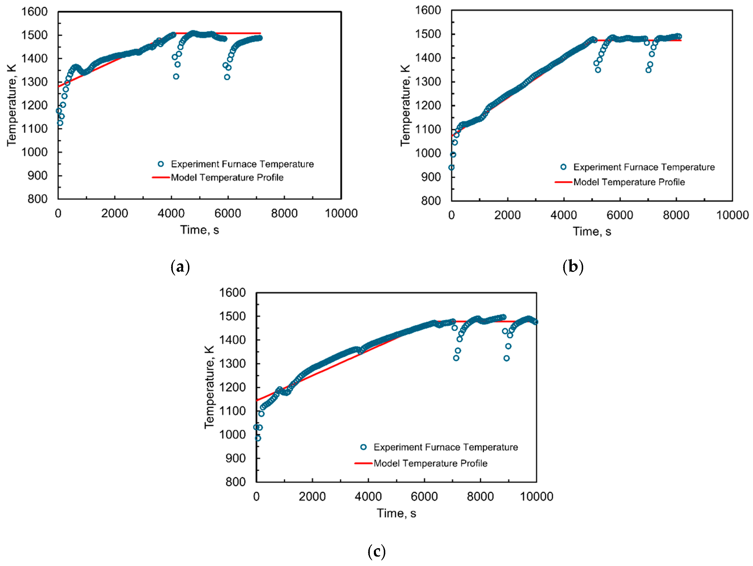
After the samples were placed inside the furnace, the atmosphere temperature increased until it reached a stable operating temperature of approximately 1200 °C as can be seen in Figure 1. At this point, the first pair of samples was removed from the furnace. The second pair was extracted after an additional 30 min of exposure, and the third pair was removed 20 min after the second pair. After removal, all samples were allowed to cool naturally in ambient air. Once cooled to room temperature, the samples were mounted in epoxy resin to facilitate subsequent microstructural and phase characterization. The process was repeated for three different furnace conditions: (1) NG–air, (2) NG–O₂ and (3) H₂–O₂.

Complementary characterization of the oxide scale was performed by Arcelor Mittal R&D using X-ray diffraction (XRD) analysis to identify the dominant oxide phases present under the different test conditions. The information obtained from this analysis was used to support the estimation of scale composition and its thermophysical properties such as density, thermal conductivity and specific heat, required in the model based on values for the three primary oxide components of scale [15]. In particular, the phase composition was incorporated to enable the conversion of oxidation data expressed in terms of mass gain per unit area into an equivalent scale thickness. This conversion allowed the oxidation kinetics, originally defined in units of mass gain (e.g., mg·cm⁻²·s⁻¹), to be consistently integrated into the numerical framework for the calculation and accumulation of oxide layer thickness over time.

The corresponding water vapor content in the furnace atmosphere was determined from the continuous measurement of dry concentrations of O₂ and CO₂ using an ABB EL3040 (ABB, Mannheim, Germany) gas analyzer. The H₂O fraction was estimated by applying combustion stoichiometry and correcting O₂ concentration to a wet basis assuming complete combustion conditions. The resulting time-dependent temperature profiles and gas compositions were used as input boundary conditions for the numerical simulations.

Boundary conditions were defined as (1) time-dependent temperature profiles based on the temperatures measured during the experiment and shown in Figure 1, and (2) species mole fractions based on the gas atmosphere compositions for each of the cases as listed in

Table 2. Composition of the reheating gas atmospheres measured during the experiments in the temperature range of 800–1200 °C.

Case	Fuel Gas	Oxidant	CO2	H2O	N2	O2
1	Methane (CH4)	Air	8.3	16.5	71.5	3.8
2	Methane (CH4)	Oxygen (O2)	36.0	51.9	8.3	3.8
3	Hydrogen (H2)	Oxygen (O2)	1.4	88.3	6.2	4.1

.

2.2. Numerical Model

2.2.1. Computational Domain, Boundary Conditions and Assumptions

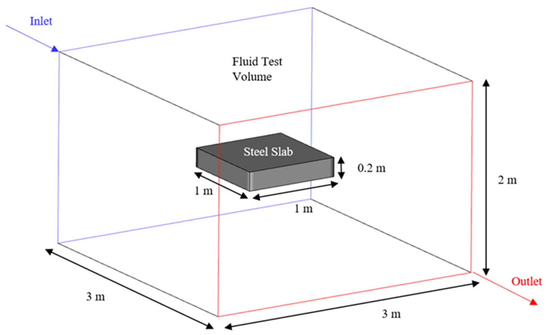
The simulation was carried out considering the simplified geometry of a virtual TGA experiment consisting of one single steel slab centered and surrounded by the fluid, which in this case was the furnace gas atmosphere. The geometry consists of a steel slab with dimensions 1 m $\times$ 1 m $\times$ 0.2 m enclosed by a surrounding fluid volume as shown in Figure 2. One of the fluid faces is defined as a velocity input with specified composition and temperature based on the experimental measurements taken during the tests, while the opposite face is a pressure outlet. The shared surface between the slab and the fluid was set up as a coupled boundary where heat flux is calculated based on the properties of the steel surface and the temperatures of the fluid adjacent to it.

2.2.2. Governing Equations

Continuity Equation

The general form of the continuity equation is solved according to Equation (1),

$${\displaystyle \frac{\partial \rho }{\partial t}}+\nabla \cdot \left(\rho \overrightarrow{v}\right)=0$$

(1)

where $\rho$ denotes fluid density, $t$ is time, and $\overrightarrow{v}$ is the velocity vector. For the individual species within a mixture, mass conservation expands to Equation (2),

$${\displaystyle \frac{\partial }{\partial t}}\left(\rho Y_i\right)+\nabla \cdot \left(\rho \overrightarrow{v}{Y}_i\right)=-\nabla \cdot \overrightarrow{J_i}+R_i$$

(2)

where $Y_i$ is the local mass fraction of each $i$ species, $\overrightarrow{J_i}$ is the diffusion flux of species $i$ and $R_i$ is the net rate of production of the $i$ species by chemical reaction. This equation is solved for the $N-1$ species where $N$ is the total number of chemical species that are present in the system.

Momentum Equation

Conservation of momentum is described by Equation (3),

$${\displaystyle \frac{\partial }{\partial t}}\left(\rho \overrightarrow{v}\right)+\nabla \cdot \left(\rho \overrightarrow{v}\overrightarrow{v}\right)=-\nabla p+\nabla \cdot \tau +\rho \overrightarrow{g}+\overrightarrow{F}$$

(3)

where $p$ is pressure, $\tau$ is the stress tensor, $\overrightarrow{g}$ is gravitational force and $\overrightarrow{F}$ is a source term that accounts for additional body forces. The stress tensor is defined by Equation (4),

$$\tau =\mu \left[\left(\nabla \overrightarrow{v}+\nabla {\overrightarrow{v}}^T\right)-{\displaystyle \frac{2}{3}}\nabla \cdot \overrightarrow{v}I\right]$$

(4)

where $\mu$ is the molecular viscosity and $I$ is the unit tensor.

Turbulence Model

The turbulence phenomenon is solved by means of the realizable $k-\epsilon$ model, which solves two equations for the turbulent kinetic energy $k$, and the rate of dissipation of turbulent kinetic energy $\epsilon$, which are expressed by Equations (5) and (6),

$${\displaystyle \frac{\partial }{\partial t}}\left(\rho k\right)+{\displaystyle \frac{\partial }{\partial x_j}}\left(\rho k{u}_j\right)={\displaystyle \frac{\partial }{\partial x_j}}\left[\left(\mu +{\displaystyle \frac{{\mu }_t}{{\sigma }_k}}\right){\displaystyle \frac{\partial k}{\partial x_j}}\right]+G_k+G_b-\rho \epsilon -Y_m+S_k$$

(5)

$${\displaystyle \frac{\partial }{\partial t}}\left(\rho \epsilon \right)+{\displaystyle \frac{\partial }{\partial x_j}}\left(\rho \epsilon u_j\right)={\displaystyle \frac{\partial }{\partial x_j}}\left[\left(\mu +{\displaystyle \frac{{\mu }_t}{{\sigma }_{\epsilon }}}\right){\displaystyle \frac{\partial \epsilon }{\partial x_j}}\right]+\rho C_1{S}_{\epsilon }-\rho C_2{\displaystyle \frac{{\epsilon }^2}{k+\sqrt{\nu \epsilon }}}+C_{1\epsilon }{\displaystyle \frac{\epsilon }{k}}{C}_{3\epsilon }{G}_b+S_{\epsilon }$$

(6)

where $C_1=\max \left[0.43,{\displaystyle \frac{\eta }{\eta +5}}\right],\eta =S{\displaystyle \frac{k}{\epsilon }}, S=\sqrt{2S_{ij}{S}_{ij}}$, $G_k$ represent the generation of turbulence kinetic energy due to the mean velocity gradients, $G_b$ is the generation of turbulence kinetic energy due to buoyancy, $Y_m$ represent the contribution of the fluctuating dilation in compressible turbulence to the overall dissipation rate. $C_2$ and $C_{1\epsilon }$ are empirical constants. ${\sigma }_k$ and ${\sigma }_{\epsilon }$ are the turbulent Prandtl numbers for $k$ and $\epsilon$, respectively. $S_k$ and $S_{\epsilon }$ are user-defined source terms.

Energy Equation

The evolution of the temperature field was obtained by solving the energy conservation described by Equation (7),

$${\displaystyle \frac{\partial }{\partial t}}\left(\rho E\right)+\nabla \cdot \left(\left(\rho E+p\right)\overrightarrow{v}\right)=\nabla \cdot \left(k_{eff}\nabla T-{\displaystyle \sum }_j{h}_j{\overrightarrow{J}}_i+{\tau }_{eff}\cdot \overrightarrow{v}\right)S_h$$

(7)

where $E$ refers to the total energy. The first three terms on the right-hand side represent the energy that is being transferred due to conduction, species diffusion and viscous dissipation, respectively. $k_{eff}$ denotes the effective thermal conductivity, ${\tau }_{eff}$ refers to the effective stress tensor. The term ${\overrightarrow{J}}_i$ represents the diffusion flux of species $j$. The term $S_h$ includes volumetric heat sources such as radiation. The radiative heat source term is modeled using the discrete ordinates method (DO), on which the radiation transfer equation is solved through Equation (8)

$$\nabla \cdot \left(I\left(\overrightarrow{r},\overrightarrow{s}\right)\overrightarrow{s}\right)+\left(a+{\sigma }_s\right)I\left(\overrightarrow{r},\overrightarrow{s}\right)=a{n}^2\frac{\sigma T^4}{\pi }+\frac{{\sigma }_s}{4\pi }{\int }_0^{4\pi }I\left(\overrightarrow{r},{\overrightarrow{s}}^{\prime }\right)\Phi \left(\overrightarrow{s}\cdot {\overrightarrow{s}}^{\prime }\right)d{\Omega }^{\prime }$$

(8)

where $\overrightarrow{r}$ and $\overrightarrow{s}$ are the position and direction vector respectively, ${\overrightarrow{s}}^{\prime }$ is the scattering direction vector, $a$ is the absorption coefficient, $n$ is the refractive index, ${\sigma }_s$ is the scattering coefficient, $\sigma$ is the Stefan–Boltzmann constant, $I$ is the radiation intensity, $T$ is the local temperature, $\Phi$ is the phase function and ${\Omega }^{\prime }$ is the solid angle [16].

Oxidation Model

Scale growth is commonly described by two main kinetic regimes, linear and parabolic, depending on the mechanism that controls the rate which can be governed primarily by gas phase reactions or solid-state diffusion. These regimes are represented by the corresponding rate equations [6,17]:

$${\displaystyle \frac{dx}{dt}}=k_l$$

(9)

$${\displaystyle \frac{dx}{dt}}={\displaystyle \frac{k_p}{2x}}$$

(10)

where $x$ is the scale thickness and $k_l$ and $k_p$ are the linear and parabolic growth rates respectively. A linear and relatively uniform increase in scale thickness is typically observed during the initial stages of oxidation. At this stage, transport through the oxide layer does not impose significant resistance, allowing iron ions to be transported rapidly to the surface. Consequently, the scaling rate, expressed as the oxide scale growth rate (dx/dt), is controlled by oxygen transfer from the atmosphere to the scale surface, as well as by the adsorption, dissociation, and reaction of oxygen with the metal.

As oxidation proceeds, the scale layer thickens, increasing the diffusion path for iron ions. This reduces the flux of ions available for oxidation reaction. Eventually, the transport of ions through the oxide layer becomes the limiting step, and the oxidation process transitions to a diffusion-controlled regime, following a parabolic rate law.

The formation of iron oxides under high-temperature conditions is integrated within the numerical model to predict iron oxide growth. This model accounts for the effect of water vapor content on the parabolic growth rate. To represent the accumulation of scale thickness, a quadratic rate expression is solved, described by Equation (11), where both linear and parabolic oxidation regimes are considered:

$${\displaystyle \frac{1}{k_l}}x+{\displaystyle \frac{1}{k_p}}{x}^2=t$$

(11)

For a non-isothermal process where the kinetic parameters vary with temperature it is convenient to use a formulation that does not depend explicitly on time. For this, Equation (11) is first differentiated, and its reciprocal is then taken. After some algebraic manipulation, the following expression described by Equation (12) is obtained:

$${\displaystyle \frac{dx}{dt}}={\displaystyle \frac{k_p{k}_l}{k_p+2k_{l}x}}$$

(12)

For the estimation of the linear and parabolic oxidation rate constants, the methodology proposed by Gaiser et al. was applied. In this approach, the onset of oxidation is first identified from the mass gain curve, allowing the experimental data to be standardized. The initial portion of the curve is used to determine the linear oxidation constant, $k_l$, while the diffusion-controlled region is fitted with a parabolic function to obtain the parabolic constant, $k_p$. The transition between both regimes is determined based on the deviation of the experimental data from the linear fit. Further details regarding the evaluation procedure can be found in [11]. The kinetic parameters used in this work were derived from thermogravimetric analysis (TGA) data reported by Haapakangas [4]. In that study, oxidation experiments were conducted on four different steel grades under natural gas–air and hydrogen–air atmospheres. From this dataset, the two steel grades with chemical compositions closest to those used in the present experimental validation were selected. The natural gas–air condition was used to validate the baseline case of the model. To include the effect of temperature, both the linear and parabolic rate constants were expressed in the Arrhenius form described by Equation (13),

$$k_{l,p}\left(T\right)=k_{0_{l,p}}\exp \left(-{\displaystyle \frac{E_a}{RT}}\right)$$

(13)

where $E_a$ is the activation energy, $R$ is the ideal gas constant, $k_{0_{l,p}}$ is the pre-exponential factor and $T$ is the temperature. The activation energies for both linear and parabolic regimes were determined using the Arrhenius expression defined in Equation (12). The temperature-dependent growth rates were obtained by performing a linear regression of the natural logarithm of the extracted growth rate constants from TGA experimental data at different temperature levels as a function of the reciprocal of temperature $\left(1/T\right)$. Since the available experimental data reported [4] corresponds to NG–air and H₂–air atmospheres, the effect of water vapor on the oxidation kinetics was incorporated through a linear correlation for the parabolic growth constant based on the work of Gaiser [11]. This formulation was implemented in the model to account for variations in water vapor concentration under different combustion atmospheres.

Table 3. Values for k_l and k_p for two different steel grades used in the scale growth model.

Steel Grade	Atmosphere	Linear Regime		Parabolic Regime
		${\mathit{E}}_{\mathit{a},\mathit{l}}$ (J/mol)	${\mathit{k}}_{0,\mathit{l}}$ (g/cm2·s)	${\mathit{E}}_{\mathit{a},\mathit{p}}$ (J/mol)	${\mathit{k}}_{0,\mathit{p}}$ (g/cm4·s2)
1045 (A)	NG–air	67,667.90	1.9787 × 10−2	75,287.92	2.6221 × 10−3
	H2–air	74,022.70	3.2118 × 10−2	104,850.63	3.6712 × 10−2
4320 (B)	NG–air	68,864.84	1.9595 × 10−2	194,307.45	48.555
	H2–air	79,778.79	4.3343 × 10−2	173,522.99	11.105

shows the values of the activation energy and along with their pre-exponential factor for the two steel grades used in the simulation.

2.2.3. Simulation Procedure

The computational domain consisted of 695,060 cells. To verify if the obtained results were independent from the mesh size, a mesh sensitivity study was conducted using three meshes with different cell sizes. First, the normalized mesh size parameter $h$ was calculated using Equation (14), with $h_1>h_2>h_3$ for the three mesh levels.

$$h={\left[{\displaystyle \frac{1}{N}}{\displaystyle {\displaystyle \sum }_{i=1}^N}\Delta V_i\right]}^{1/3}$$

(14)

where $\Delta V_i$ is the cell volume for a three-dimensional mesh. Then, the refinement ratio was estimated by using Equation (15), representing how the discretized domain is refined for each level of refinement.

$$r_{32}={\displaystyle \frac{h_3}{h_2}}$$

(15)

The refinement ratio must follow the condition $r\ge 1.1$. For our grid dependence study, we obtained a refinement ratio of 1.3 for the two levels of refinement. Next, the order of convergence for the variable of interest, in this case mass gain, was determined using results from the three meshes using Equation (16),

$$p={\displaystyle \frac{\ln \left(\frac{f_3-f_2}{f_2-f_1}\right)}{\ln \left(r\right)}}$$

(16)

where $p$ represents the truncation error for the variable of interest for the refinement levels. Using the normalized mesh parameter, the value of the variable of interest can be estimated using Richardson extrapolation as shown in Equation (17):

$$f_{h=0}=f_1+{\displaystyle \frac{f_3-f_2}{r^p-1}}$$

(17)

Finally, the grid convergence index (GCI) is calculated for two refinement levels among the three meshes using Equation (18),

$$GCI={\displaystyle \frac{F_s\left|e\right|}{r^p-1}}$$

(18)

where $F_s$ is a safety factor, for this case of 1.25, and $\left|e\right|$ is the absolute error [18].

The solution on the fine grid had a result of 434.96 mg/cm² and the extrapolated value is 453.6 mg/cm² which gives a grid convergence index of 6% when going from the medium to the fine grid. Based on this, the solution can be considered independent of grid size. Complete results for the grid convergence study are shown in

Table 4. Results of the grid convergence study over three different meshes.

	No. of Cells	$\mathit{\varphi }$	r	p	GCI	${\mathit{\varphi }}_{\mathit{e}\mathit{x}\mathit{t}\mathit{r}\mathit{a}\mathit{p}\mathit{o}\mathit{l}\mathit{a}\mathit{t}\mathit{e}\mathit{d}}$
Mesh 1	695,060	434.96	-		6%
Mesh 2	316,368	412.27	1.3	3.001	14%	453.90
Mesh 3	144,000	362.42	1.3		-

.

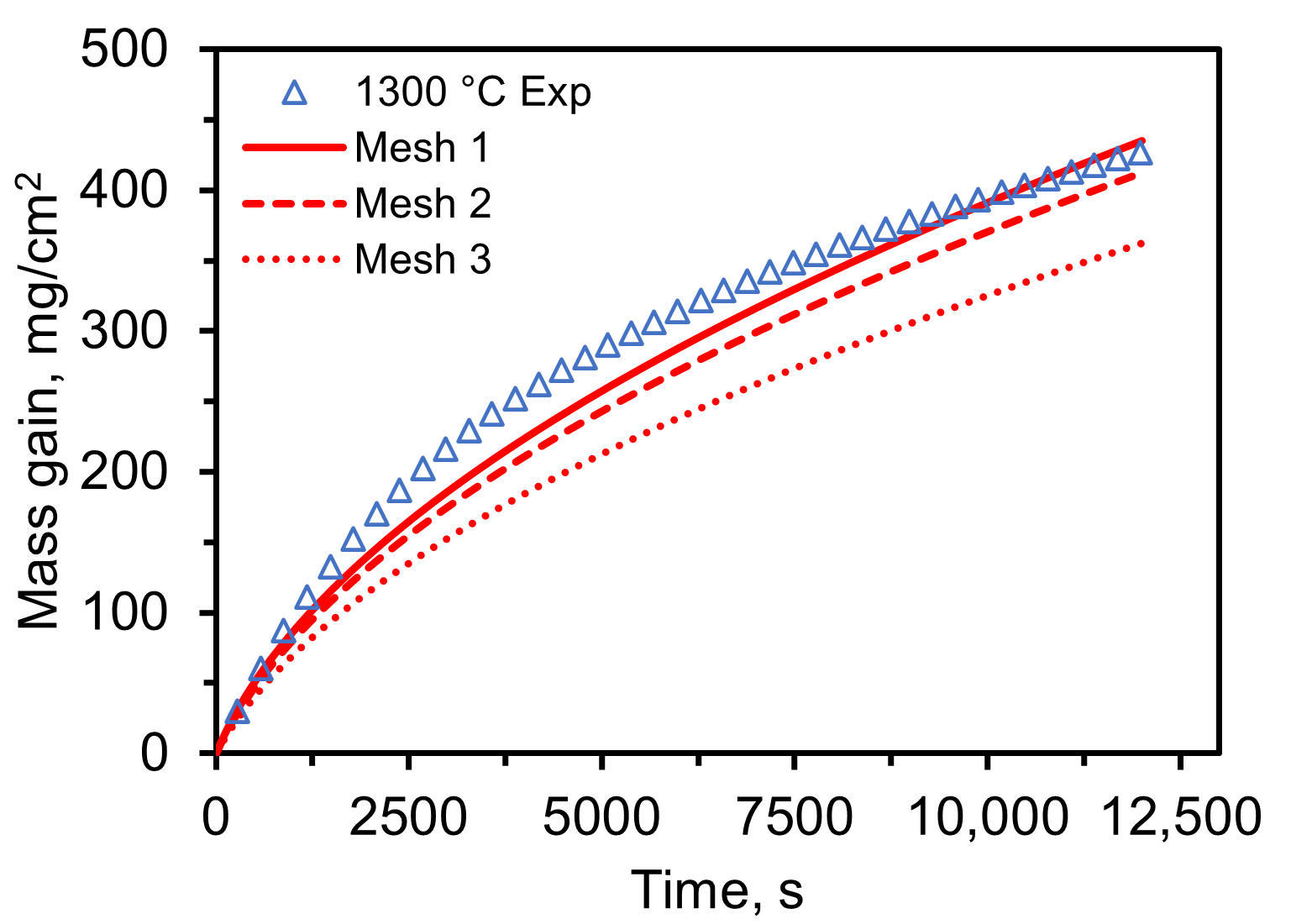
Figure 3 shows that the finer mesh provides the closest agreement with the experimental data, particularly at longer times. Although the CGI analysis suggests that intermediate mesh could be selected to reduce computational cost, the improved accuracy observed with the finer mesh justifies its use. Therefore mesh 3 is used in the present study.

Numerical models were solved using commercial code ANSYS Fluent 2024R2, using a coupled algorithm. The convergence criteria were established for the residuals of all the variables as 10⁻⁴, except for energy and DO residuals, which were set as 10⁻⁶. These convergence criteria were reached at every time step during the transient simulation for all the cases. The mixed oxidation model formulation was implemented through a user-defined function (UDF). The UDF evaluates the oxidation rate at every time step using the local temperature-dependent kinetic parameters. The scale thickness is then incrementally updated and accumulated over time. The resulting thickness values are stored in user-defined memory (UDM), which allows the evolution of scale growth to be tracked and later extracted for post-processing and analysis.

The thermophysical properties of the materials and chemical species used in the numerical model are listed in

Table 5. Thermophysical properties of the solid materials used in the numerical model [15,20].

Material	Density (kg·m−3)	Specific Heat (J·kg−1·K−1)	Thermal Conductivity (W·m−1·K−1)
Scale	5633 [15]	750.40 [15]	2.8 [15]
Steel	8030	502.48	Polynomial [20]

. For the thermophysical properties of the gas mixture, temperature-dependent specific heat capacities of the gas species were calculated using NASA polynomials [19] and mixture density was calculated based on the incompressible ideal gas law [16].

The thermophysical properties of the scale were estimated using the mixture formulation described by Equation (19) and based on the oxide composition of the scale layer obtained by X-ray diffraction analysis and according to the individual oxides thermophysical properties listed in Table 5.

To consider the thermal resistance imposed by the layer of scale, an effective resistance was calculated using the thermal resistance concept expressed by Equation (19),

$$k_{eff}={\displaystyle \frac{L_{steel}}{\frac{L_s}{k_s}+\frac{L_{steel}}{k}}}$$

(19)

where $L_{steel}$ is the thickness of the cell is defined as a solid dmain, $L_s$ is the scale thickness, $k_s$ is the thermal conductivity of scale and $k$ is the steel thermal conductivity.

3. Results

3.1. Experimental Scale Thickness

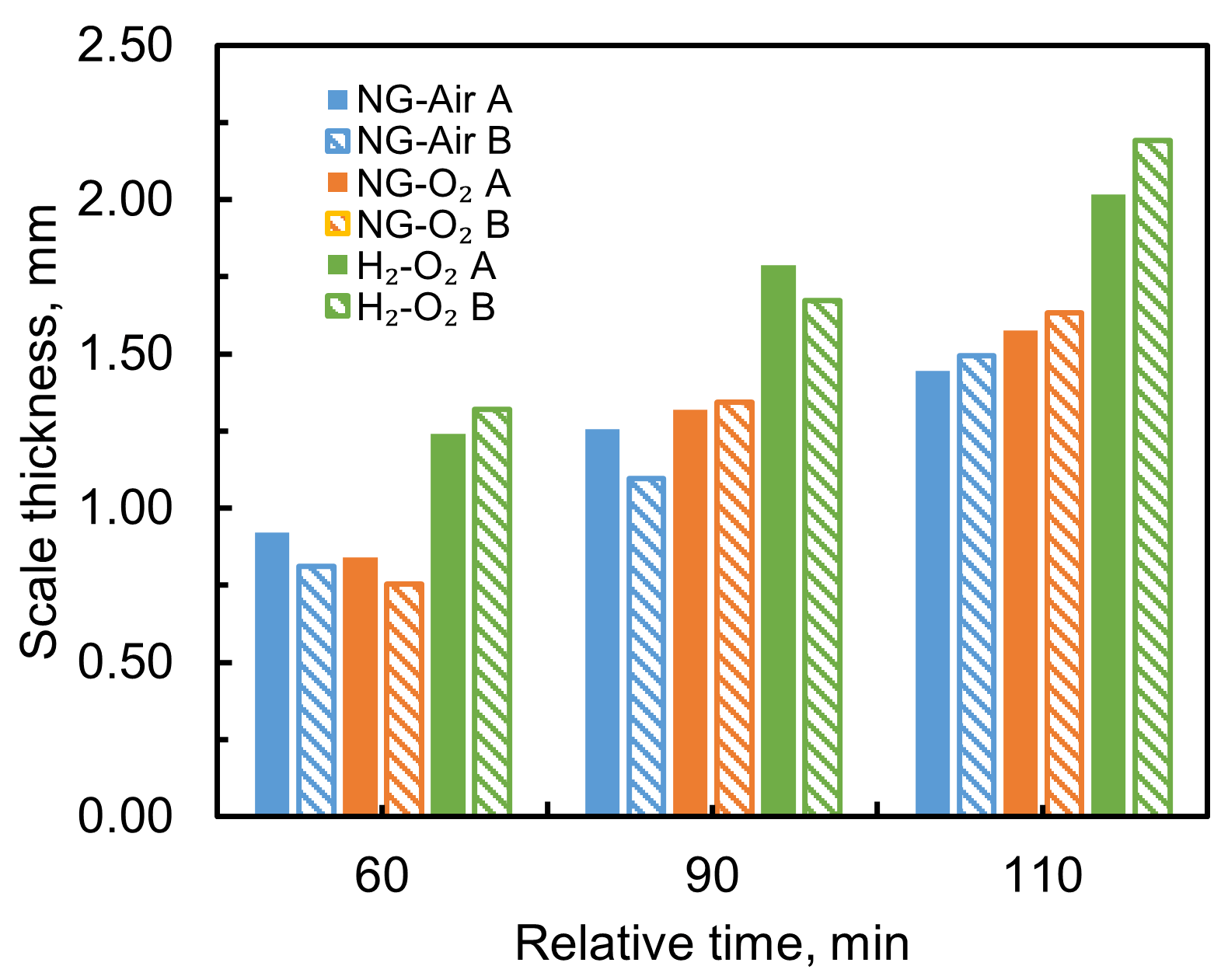
To measure the thickness of the oxide scale formed during the experiments, images of the sample cross-sections were captured. These images were processed to enhance contrast and sharpen the features, facilitating a clearer identification of the scale metal interface. Ten evenly spaced measurements were taken along the top portion of each sample. Using the software ImageJ v. 1.54g, the images were calibrated by relating pixel dimensions to a reference measurement obtained from a conventional ruler placed on the cut samples. The average of the ten measurements was then used as the representative scale thickness. Figure 4 shows the scale thickness results for the three experiments conducted under natural gas air and oxygen-enriched conditions with both natural gas and hydrogen. The results indicate that the oxide scale grows with increasing residence time, and that hydrogen atmospheres produce a noticeably thicker scale compared to natural gas.

3.2. Simulation Results

3.2.1. Model Calibration

In this study, several test conditions were simulated using the numerical model with the implemented oxidation model. The objective was to evaluate the model behavior by calibrating the kinetic parameters with thermogravimetric analysis (TGA) experimental results reported in the literature by Haapakangas [4]. The conditions selected from the work of Haapakangas correspond to the combustion of natural gas and hydrogen with air as oxidant at three temperature levels: 1150, 1230, and 1300 °C. These two baseline cases were defined to evaluate the temperature-dependent oxidation kinetics extracted from the experimental data.

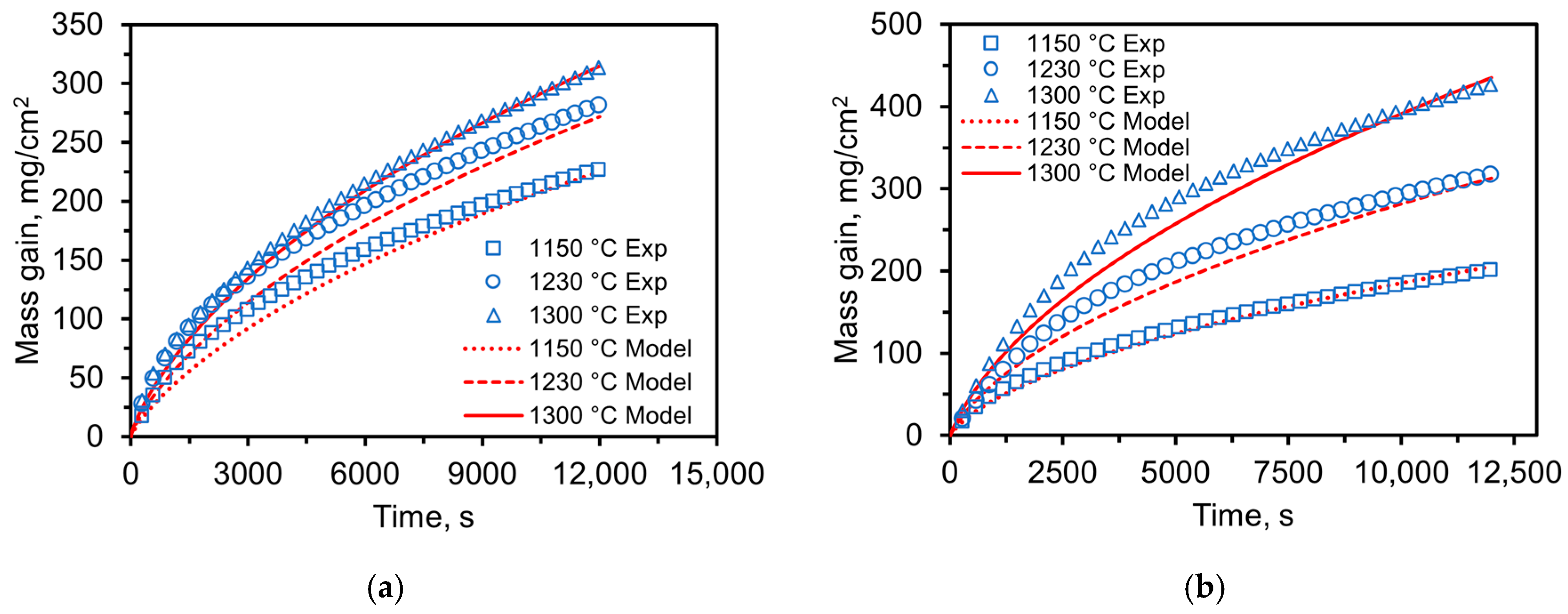
Figure 5 shows the comparison between the temperature-dependent kinetic parameters obtained from the model and the TGA experimental results for two different steel grades. For the three temperature levels analyzed, a strong agreement between the model predictions and the experimental measurements can be observed. This is further supported by R² values exceeding 0.991 for all temperatures and both steel grades, indicating a good correlation between predicted and measured mass gain. The resulting mass gain curve is represented as a continuous function due to the use of a mixed kinetic model that accounts for both linear and parabolic oxidation regimes. This formulation avoids the need to explicitly define a transition time between the two regimes, as the growth rate expression does not depend directly on time.

3.2.2. Model Validations

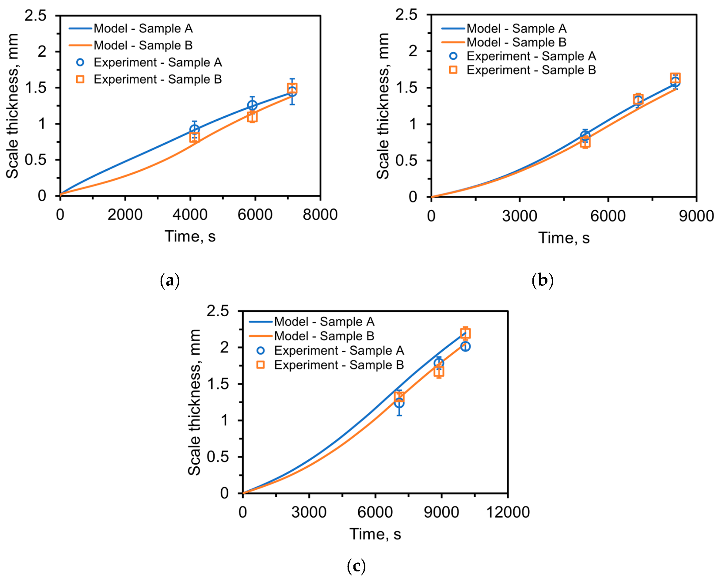
Figure 6 shows the comparison between the predicted oxide scale thickness obtained from the oxidation model and experimental measurements for both Sample A and Sample B under three different combustion atmospheres: NG–air, NG–O₂, and H₂–O₂. It can be seen that for all cases, the scale thickness increases with residence time, and the model captures the general growth trend observed in the experiments.

For Case 1 in Figure 6a both samples exhibit a gradual increase in scale thickness with time, reaching approximately 1.42 mm for Sample A and 1.38 mm for Sample B at the longest residence time. The model predictions show good agreement with the experimental measurements, with deviations generally below 10% for all samples. For Sample A, the predicted trend closely follows the experimental data throughout the entire time range, with an average relative error of approximately 1%. For Sample B, the model slightly underpredicts the scale thickness at intermediate times around 4140 s, while the predicted values remain within 0.09 mm difference of the experimental measurements. These results indicate that the model captures the oxidation kinetics reasonably well under conventional NG–air combustion conditions, which is the baseline case.

For Case 2 under NG–O₂ combustion in Figure 6b, an overall increase in oxidation rate is observed compared to the NG–air case. At the longest residence time, the measured scale thickness reaches approximately 1.55 mm for Sample A and 1.48 mm for Sample B, representing an increase of about 9.2% for Sample A and 9.3% for Sample B relative to the NG–air operation. The model successfully reproduces this increased oxidation tendency, with predicted values deviating by less than 10% from the experimental measurements. The overall agreement remains good, suggesting that the model captures the influence of higher water vapor content on scale growth.

For the final Case 3 with H₂–O₂ combustion atmosphere shown in Figure 6c the highest oxidation rates among the three cases are observed. The scale thickness increases more rapidly with time, reaching approximately 2.2 mm for Sample A and 2.05 mm for Sample B at the final sample measured. Compared to the baseline NG–air operation condition, this represents an increase of approximately 39.6% for Sample A and 46.8% for Sample B in final scale thickness. The model predictions follow the experimental trends closely, particularly at longer residence times, where the predicted and measured values differ by less than 0.2 mm for both samples. Minor discrepancies are observed at initial times, where the model predicts slightly higher scale thickness values for Sample A by approximately 0.22 mm. In relative terms, the average deviation between the model predictions and experimental measurements is on the order of 10%, with maximum deviations of up to approximately 17% observed under specific conditions (Sample A, H₂–O₂). The larger discrepancies at early times are attributed to partial scale loss prior to measurement, likely due to spallation during sample transport and handling. While measurements were taken to preserve samples during sample transport and handling, this effect could not be fully eliminated and may lead to an underestimation of the initial scale thickness. Nevertheless, the model captures the overall trends and scale thickness evolution at longer residence times, where agreement with experimental data improves.

The comparison between experimental measurements and model predictions across the three combustion atmospheres demonstrates that the oxidation model can capture the main trends in oxide scale growth under different furnace conditions. The results also highlight the influence of combustion atmosphere on oxidation behavior, with oxygen-enriched and hydrogen-fueled operations leading to increased scale formation compared to conventional NG–air combustion. The increased oxidation observed under hydrogen combustion conditions can be primarily attributed to the significantly higher water vapor content in the furnace atmosphere. Water vapor acts as an additional oxidizing species, promoting the formation of iron oxides through reactions that facilitate the transport of oxygen to the metal surface. Compared to atmospheres with lower water vapor content, the presence of H₂O increases the effective oxygen potential and accelerates oxidation kinetics, particularly in the parabolic regime. The results obtained in this study are consistent with previous findings reported in the literature, where increased H₂O concentrations in combustion products have been associated with higher oxidation rates and thicker oxide layers. Therefore, the increased scale thickness observed under H₂–O₂ conditions can be directly linked to the combined effect of high temperature and increased water vapor content inherent to hydrogen combustion. Under these conditions, a maximum scale growth rate for the two steel grades of 0.012–0.013 mm/min (or a maximum thickness of 2.02–2.19 mm) was observed.

4. Conclusions

The presented results demonstrate that the implemented oxidation model provides a reliable representation of high-temperature scale growth under different combustion atmospheres relevant to reheating furnace operation in the temperature range of 800–1200 °C. The comparison with TGA data confirms that the temperature-dependent kinetic parameters incorporated in the mixed model formulation can reproduce the oxidation behavior of the analyzed steel grades across the investigated temperature range (800–1200 °C). Furthermore, the comparison with experimental scale thickness measurements shows that the model successfully captures the evolution of oxide growth for NG–air, NG–O₂, and H₂–O₂ combustion atmospheres, maintaining an average prediction error of approximately 6%. The simulations also highlight the strong influence of combustion atmosphere on oxidation behavior, with oxygen-enriched and hydrogen-fueled conditions leading to significantly higher scale formation compared to conventional NG–air operation. These findings indicate that the proposed modeling approach can serve as a predictive tool for assessing oxidation behavior under emerging low-carbon combustion strategies and for supporting the optimization of reheating furnace operation as the steel industry transitions toward hydrogen-based and oxygen-enriched heating technologies. The following main conclusions can be drawn:

•

The implemented methodology successfully reproduces temperature-dependent oxidation kinetics observed in TGA experiments for the analyzed steel grades.

•

The mixed kinetic formulation effectively represents both linear and parabolic oxidation regimes without requiring an explicit transition time between them.

•

Model predictions show good agreement with experimental scale thickness measurements, with an average error of approximately 6% across all cases; however, deviations vary depending on atmosphere and time, with maximum errors of up to approximately 17% observed under specific conditions.

•

Oxygen-enriched combustion (NG–O₂) leads to an increase in scale formation, resulting in approximately 9% higher scale thickness compared to the NG–air baseline operation.

•

Hydrogen-based combustion (H₂–O₂) produces the highest scale growth, with scale thickness increasing by up to ~40–47% relative to conventional NG–air operation.

•

The model captures the general trend of increasing scale growth with residence time under all combustion atmospheres considered.

The present model is subject to the following limitations: First, the computational domain is based on a simplified single slab geometry, which does not capture interactions present in industrial furnaces that can accommodate multiple slabs or billets. Second, the kinetic parameters employed are derived and calibrated within a specific range of temperatures and gas compositions; extrapolation beyond the validated water vapor content range may introduce additional uncertainty. Finally, the model does not account for mechanical effects such as scale cracking or spallation, which can influence the effective scale thickness, particularly during handling and transient conditions.

References

1. World Steel Association. World Steel in Figures 2025; World Steel Association: Brussels, Belgium, 2025; Available online: https://worldsteel.org/media/publications/world-steel-in-figures-2025 (accessed on 16 March 2026).
2. Airaksinen, S.; Haapakangas, J.; Gyakwaa, F.; Heikkinen, E.P.; Fabritius, T. Utilization of hydrogen fuel in reheating furnace and its effect on oxide scale formation of low-carbon steels. Int. J. Hydrog. Energy 2025, 140, 1212–1220. [Google Scholar] [CrossRef] [Scilit]
3. Schwarz, S.; Daurer, G.; Plank, B.; Krull, H.G.; Szittnick, A.; Lakhdari, M.A.; Collin, S.; Gasca, P.; Chauveau, E.; Deville-Cavellin, C.; et al. A comparative experimental analysis of the scale formation of various steel grades during reheating under hydrogen and natural gas air–fuel and oxy–fuel combustion conditions. Int. J. Hydrog. Energy 2025, 101, 1105–1115. [Google Scholar] [CrossRef] [Scilit]
4. Haapakangas, J.; Riikonen, S.; Airaksinen, S.; Heikkinen, E.P.; Fabritius, T. Oxide scale formation on low-carbon steels in future reheating conditions. Metals 2024, 14, 189. [Google Scholar] [CrossRef] [Scilit]
5. Gyakwaa, F.; Airaksinen, S.; Visuri, V.V.; Heikkila, A.; Fabritius, T. Influence of Hydrogen Fuel Mixtures on the Oxide Scale Formation of Low-Carbon Steels in Reheating Furnace Conditions. Steel Res. Int. 2025, 2500248. [Google Scholar] [CrossRef] [Scilit]
6. Young, D.J. High Temperature Oxidation and Corrosion of Metals; Elsevier: Amsterdam, The Netherlands, 2008; Volume 1. [Google Scholar]
7. Schluckner, C.; Gaber, C.; Demuth, M.; Forstinger, S.; Prieler, R.; Hochenauer, C. CFD-model to predict the local and time-dependent scale formation of steels in air-and oxygen enriched combustion atmospheres. Appl. Therm. Eng. 2018, 143, 822–835. [Google Scholar] [CrossRef] [Scilit]
8. Landfahrer, M.; Schluckner, C.; Prieler, R.; Gerhardter, H.; Zmek, T.; Klarner, J.; Hochenauer, C. Numerical and experimental investigation of scale formation on steel tubes in a real-size reheating furnace. Int. J. Heat Mass Transf. 2019, 129, 460–467. [Google Scholar] [CrossRef] [Scilit]
9. Gómez, M.A.; Casal, J.M.; González-Gil, L.; Álvarez-Bermúdez, C.; Porteiro, J. CFD-integrated kinetic model for high-temperature iron oxidation in multispecies reactive environments. Materialia 2025, 42, 102464. [Google Scholar] [CrossRef] [Scilit]
10. Pineda Huitron, R.M.; López Ramírez, P.E.; Vuorinen, E.; Jalali, P.N.; Pelcastre, L.; Karkkainen, M. Scale formation on HSLA steel during continuous casting part I: The effect of temperature–time on oxidation kinetics. Metals 2020, 10, 1243. [Google Scholar] [CrossRef] [Scilit]
11. Gaiser, G.; Peter, P.; Christian, B.; Sergiu, I. Scaling Behavior and Surface Quality of High-Strength Low-Alloy Steels with Higher Levels on Cu, Sn, and Ni Under Slab Reheating Conditions. High Temp. Corros. Mater. 2025, 102, 8. [Google Scholar] [CrossRef] [Scilit]
12. Gaiser, G.; Presoly, P.; Bernhard, C. High-temperature oxidation of steel under linear flow rates of air and water vapor—An experimental determined set of data. Metals 2023, 13, 892. [Google Scholar] [CrossRef] [Scilit]
13. Von Scheele, J.; Alshawarghi, H.; Murphy, J.; Diggins, P.; Salvador B, O. Decarbonization through proven energy-efficient solutions and use of hydrogen in reheat furnaces. In Proceedings of the Iron & Steel Technology Conference (AISTech 2024), Columbus, OH, USA, 6–9 May 2024. [Google Scholar] [CrossRef] [Scilit]
14. Von Scheele, J. Oxyfuel combustion with hydrogen in the steel, non-ferrous, and glass industries. In Proceedings of the International Flame Research Foundation–TOTeM Meeting, Essen, Germany, 27–28 May 2022. [Google Scholar]
15. Torres, M.; Colas, R. A model for heat conduction through the oxide layer of steel during hot rolling. J. Mat. Process. Technol. 2000, 105, 258–263. [Google Scholar] [CrossRef] [Scilit]
16. Ansys, Inc. Ansys Fluent Theory Guide, Ansys; Ansys, Inc.: Cannonsburg, PA, USA, 2013; p. 3187. [Google Scholar]
17. Tammann, G. Über Anlauffarben von metallen. Z. Anorg. Und Allg. Chem. 1920, 111, 78–89. [Google Scholar] [CrossRef] [Scilit]
18. Roache, P.J. Verification and Validation in Computational Science and Engineering; Hermosa: Albuquerque, NM, USA, 1998; Volume 895. [Google Scholar]
19. McBride, B.J.; John, H. NASA Glenn Coefficients for Calculating Thermodynamic Properties of Individual Species; National Aeronautics and Space Administration, John, H. Glenn Research Center at Lewis Field: Cleveland, OH, USA, 2002.
20. Peet, M.J.; Hasan, H.S.; Bhadeshia, H.K.D.H. Prediction of thermal conductivity of steel. Int. J. Heat Mass Transf. 2011, 54, 2602–2608. [Google Scholar] [CrossRef] [Scilit]
Figure 1. Comparison of time-dependent temperature profiles used as boundary conditions and furnace temperature measured during the experiments for different atmospheres: (a) NG–air, (b) NG–O2 and (c) H2–O2.
Metals 16 00534 g001
Figure 2. Computational domain and boundary conditions of the virtual thermogravimetric experiment.
Metals 16 00534 g002
Figure 3. Comparison of mass gain curves for steel grade A under NG-air conditions at constant temperature of 1300 °C for three different mesh refinement levels and experimental results.
Metals 16 00534 g003
Figure 4. Experimental measurement of scale thickness as a function of time for three different atmosphere conditions, NG–air, NG–O2 and H2–O2, for three different residence times.
Metals 16 00534 g004
Figure 5. Mass gain calculated by the model, (a) Grade A and (b) Grade B and experimental data [4], for three different temperature levels.
Metals 16 00534 g005
Figure 6. Comparison of scale thickness calculated with the oxidation model with experimental measurements for all experiments: (a) NG–air, (b) NG–O2 and (c) H2–O2.
Metals 16 00534 g006