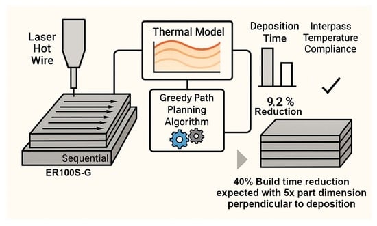
Path Planning for Rapid DEDAM Processing Subject to Interpass Temperature Constraints

Abstract

Directed energy deposition (DED) additive manufacturing (AM) enables the production of components at a high deposition rate. For certain alloys, interpass temperature requirements are imposed to control heat accumulation and microstructure transformation, as well as to minimize distortion under varying thermal conditions. A typical strategy to comply with interpass temperature constraints is to increase the interpass dwell time, which can lead to an increase in the total deposition time. This study aims to develop an optimized tool path that ensures interpass temperature compliance and reduces overall deposition time relative to the conventional sequential deposition path during the DED process. To evaluate this, a compact analytic thermal model is used to predict the thermal history during laser-based directed energy deposition (DED-LB/M) hot wire (lateral feeding) of ER100S-G, a welding wire equivalent to high yield steel. A greedy algorithm, integrated with the thermal model, identifies a tool path order that ensures compliance with the interpass requirement of the material while minimizing interpass dwell time and, thus, the total deposition time. The proposed path planning algorithm is validated experimentally with in situ temperature measurements comparing parts fabricated with the baseline (sequential) deposition path to the modified path (resulting from the greedy algorithm). The experimental results of this study demonstrate that the proposed path planning algorithm can reduce the deposition time by 9.2% for parts of dimensions 66 mm × 73 mm × 16.5 mm, comprising 15 layers and a total of 300 beads. Predictions based on the proposed path planning algorithm indicate that additional reductions in deposition time can be achieved for larger parts. Specifically, increasing the (experimentally validated) part dimension perpendicular to the deposition direction by five-times is expected to result in a 40% reduction in deposition time.

1. Introduction

Laser-based directed energy deposition (DED-LB/M) hot wire (lateral feeding), also known as laser hot wire (LHW) DED, is a prominent additive manufacturing (AM) technique that combines a laser heat source with an electrically preheated filler wire to deposit material in a layer-by-layer fashion. The integration of the hot wire and laser enables higher deposition rates and increased energy efficiency compared to traditional laser deposition processes [1]. As a result, LHW has gained considerable attention for its potential applications in the aerospace, automotive, and energy sectors, where high-performance, complex, and custom-designed components are in demand [2].

Numerous prior studies have explored the influence of key process parameters on process stability in LHW cladding and DED. Peng et al. [3] found that, for single-pass LHW cladding, the preheat temperature of the hot wire was a primary contributor to the deposition quality, and they also identified the optimal wire feed rate and current for their specific study. The same group [4] also classified wire transfer behavior into three separate models: fuse model, wire hit model, and continuous model. The fuse model resulted in arc and spatter, the wire hit model deposited non-straight tracks, and the continuous model was the ideal state of LHW cladding that produced a stable deposition process. Liu et al. [5] concluded that the wire feeding orientation and wire tip position were critical parameters for LHW cladding and stated that wire feeding with the tip at the rear of the melt pool gave the optimal position. This same group [6] later studied the effects of wire current and laser power on LHW cladding and found that the wire current played a critical role in process stability; e.g., higher voltages resulted in arcing and spattering, reducing the stability of the process. Laser power affected stability, but its effect was not as impactful as wire current. Huang et al. [7] applied the Taguchi method to select process parameters for the LHW cladding of martensitic steel, where the volumetric defect ratio was used to characterize the integrity of cladding layers. They found that the wire current and feed rate had a significantly greater influence on the deposition quality than scanning speed and laser power. Kottman et al. [8] implemented a closed loop control system and monitored resistive heating to suppress the occurrence of arcing during deposition, leading to enhanced process stability. Zhang et al. [9] also found that resistive heating played a dominant role in process stability. In addition, the wetting angle, cladding height, and dilution rate were all affected by the material deposition density, demonstrating the combined effects of material feed rate and scanning speed. Budde et al. [10] conducted an experimental study on process parameters for single-weld seams using the LHW cladding of AISI 52100. The process stability was shown to be dependent on the wire feed rate, current, and welding speed. They found that at certain feed rates, a stable welding process occurred regardless of the other parameters. At higher feed rates, slower welding speeds were needed, while at lower feed rates, smooth wire transfer was present at lower currents. Stavropoulos et al. [11] tracked heat accumulation in LHW-DED through the use of a vision-based monitoring system that captured melt pool dimensions. They proposed a real-time process control that simultaneously tuned laser power and cooling time.

One of the most significant challenges in LHW-DED is the control of the interpass temperature. The interpass temperature is a critical issue in welding. It is defined as the temperature of the material in the weld area immediately before the next weld pass occurs [12]. High interpass temperatures have adverse effects on the microstructure and mechanical properties for a variety of metal alloys [12,13,14,15]. This issue is equally critical for LHW due to similar microstructure and mechanical property concerns. In general, the interpass temperature gradually increases as heat accumulates during the build process when the same processing conditions are maintained. This is an irreversible trend until heat input and heat dissipation have reached a balance during the process [16].

Interpass temperature effects have been studied on a multitude of additive manufacturing systems, including wire arc additive manufacturing (WAAM), with either gas metal arc welding (GMAW) or tungsten arc welding (GTAW). Geng et al. [17] stated that controlling the interpass temperature was essential to avoid bead defects and reduce cross-sectional geometry variations. Ma et al. [18] conducted an experimental study of titanium aluminide alloys with GTAW and found that the interpass temperature significantly affected microhardness, microstructure, and local chemical composition. Similarly, Shen et al. [19] conducted a study for WAAM of iron aluminide alloys and demonstrated the effects of interpass temperature on the longitudinal cracking, yield stress, and elongation. For WAAM of aluminum, Derekar et al. [20] found that the interpass temperature had a significant effect on porosity formation. Poulain et al. [21] studied the effect of interpass temperature on the microstructure of super duplex stainless steel using cold wire gas metal arc (CW-GMA) additive manufacturing. For this alloy, they determined that the interpass temperature influenced thermal accumulation and microstructural details, but the effect on mechanical properties was minimal. Ren et al. [22] found that maintaining the stability of melt pool conditions is critical for consistent cooling and solidification rates in DED by minimizing degradation in build accuracy and improving microstructure homogeneity. They proposed using deep reinforcement learning to modulate laser power during the DED process without the use of physical sensors or closed loop in-process monitoring.

Interpass temperature requirements are commonly defined by the specific material and process involved. One material of interest in naval applications is ER100S-G (or ER100S-1, depending on specifics), which is often used for welding and cladding on HY-80 steel, as well as for the LHW fabrication of components. This material has a required interpass temperature of 121–177 °C (250–350 °F) [23,24,25]. To meet the interpass temperature requirement, interpass dwell time is often needed, sometimes with additional forced cooling [26]. Based on finite element simulations of the thermal behavior of ER70S-6 wire (carbon steel filler) during the WAAM process, Montevecchi et al. [27] developed an algorithm to calculate the interpass dwell time required to meet the interpass temperature requirements. Vázquez et al. [28] proposed a method of forced cooling to control the interpass temperature for WAAM of Ti-6Al-4V parts, where internal water cooling was applied to the build plate to quickly decrease the temperature between depositions, reducing the required dwell time significantly. However, a large amount of forced cooling may not be feasible, while simply increasing the interpass dwell time will increase the overall build time.

This study proposes utilizing reduced-order thermal models to enable path plan optimization in order to meet the interpass temperature requirements while reducing the required interpass dwell times. Based on thermo-mechanical analysis of the laser-aided additive manufacturing (LAAM) process, the study by Ren et al. [29] showed that path planning could also have a significant effect on mechanical property distribution. He et al. [30] proposed a scan optimization approach utilizing a combination of thermal models and control-based techniques for laser powder bed fusion (LPBF), aimed at homogenizing temperature to reduce distortion. This effort projected a finite difference model to lower dimensions through radial basis functions and then solved a minimization problem through an exhaustive examination over control–system matrix elements to select path planning. Although projections using the radial basis functions allowed for a reduction in the model dimensions, checking each matrix element in the minimization process could still be computationally expensive. Song et al. [31] demonstrated that intersection path planning could be utilized to reduce height error and increase internal stability for WAAM. A model was developed to eliminate unnecessary paths and to minimize height differences at intersections by optimizing bead overlap. Zhao et al. [32] proposed a combination of a contour offset method and zigzag pathing, where a polygon trapezoidal partitioning algorithm was used to partition complex polygons into multiple subregions. Then, a zigzag path method was used to fill these areas while reducing the staircase effect. All areas were then recombined and converted into robot tool paths and compared to traditional contour offset path planning. This method produced components with no pore defects with high geometric reduction. Nguyen et al. [33] developed a model to characterize multi-bead overlapping. Through analyzing several path plans, e.g., zigzag and contour patterns, they were able to find the optimal overlapping distance for these hybrid tool path patterns.

In this study, a novel approach is introduced for controlling the interpass temperature and reducing build time in DEDAM of ER100S-G wire through strategic path planning. Unlike traditional methods that rely solely on process parameter tuning or computationally intensive finite element (FE) simulations, we propose the use of a simplified thermal model—based on a modified version of Rosenthal’s solution—as a reduced-order predictor of the temperature distribution. Furthermore, this thermal model is then integrated with a greedy path planning algorithm that selects the deposition order based on local optimization of interpass temperature compliance, rather than global optimization over the entire build sequence. This represents a significant shift in methodology, reframing path planning as a thermal control tool in addition to its traditional role in geometric fidelity and efficiency. By avoiding full-scale integer programming and instead leveraging local decision making, the proposed method significantly reduces computational costs while effectively satisfying interpass temperature requirements. Finally, an experimental study is conducted in this study to evaluate the resulting scan path for test coupons in reducing the total build time while complying with the interpass temperature control requirement for ER100S-G wire. In situ temperature measurements are taken using a calibrated pyrometer for experimental validation of the interpass temperatures. The experimental build time under the modified scan path, resulting from the proposed combination of the greedy algorithm and simplified thermal model, is then compared with the build time under the sequential scan path. The rest of this paper is organized as follows: Section 2 presents the materials and methods. Results and discussions are given in Section 3. Conclusions are then drawn at the end.

2. Materials and Methods

2.1. LHW-DED AM Process

Figure 1 depicts the robotic LHW-DEDAM system utilized in this study. The energy input is provided by a YLR-12000-C IPG Photonics Ytterbium fiber laser (IPG Photonics, Oxford, MA, USA) (wavelength: 1070 nm) integrated with a 200 µm process fiber. The output energy is collimated and focused using water-cooled, reflective parabolic mirrors with focal lengths of f = 150 mm and f = 600 mm. During operation, the laser beam is defocused by approximately 115 mm beyond the focal point, resulting in a beam diameter of approximately 3.9 mm, as determined using beam caustic measurements at the focal point. The system includes a 6-axis ABB IRB-6700 150/3.2 robot (ABB, Zurich, Switzerland) integrated with an ABB IRBP A-750/1450 two-axis workpiece positioner (ABB, Zurich, Switzerland). A Lincoln Electric Power Wave^® R500 and STT^® control module are used to prevent arc initiation during processing. The LHW system incorporates a Laser Mechanisms FiberSCAN HR laser processing head (Laser Mechanisms, Novi, MI, USA), which oscillates the laser beam at 14 Hz, with a center-to-center scanning width of 2.5 mm perpendicular to the travel direction.

The LHW system follows a five-stage process for each bead deposition: Preheat, Pre-Fill, Main-Deposition, End-Fill, and End-Delay. The laser power, wire feed rate, and duration for each stage used in this study are detailed in

Table 1. Process parameters developed for each stage.

Stage	Wire Feed Rate	Laser Power	Laser Travel Speed	Stage Duration
Preheat	0 mm/s	7.5 kW	-	0.1 s
Pre-Fill	30 mm/s	7.5 kW	-	0.25 s
Main-Deposition	60 mm/s	7.5 kW	13 mm/s	Determined by bead length
End-Fill	45 mm/s	7 kW	-	0.4 s
End-Delay	0 mm/s	2 kW	-	0.5 s

. During the Preheat phase, the laser irradiates the substrate before wire deposition begins. The robot arm remains stationary without wire feeding, while the laser oscillates at the specified frequency. In the Pre-Fill stage, the wire feed is initiated to start bead deposition, while the robot arm stays stationary with the oscillating laser. During the Main-Deposition phase, the wire feed rate increases, and the robot arm moves along the bead path at a default travel speed of 13 mm/s. In the End-Fill phase, the robot arm stops moving, while the wire continues to feed at a reduced rate. In the final End-Delay phase, the laser power decreases, and the wire feed stops, completing the process.

The hot wire supply in this study operates with an average current of 99.83 A at 1.80 V, and the wire diameter is 1.14 mm, corresponding to 0.045-inch diameter welding wire commonly found in the United States and Canada. The length of the wire under current (from the contact tip to the melt pool) is 22.5 mm. These parameters are summarized in

Table 2. Hot wire parameters.

Current Supplied	99.83 A
Average Voltage	1.80 V
Wire Diameter	1.14 mm
Wire Length with Current Applied	22.5 mm

. The shielding gas used in the experiment is Argon with a flow rate of 0.005 m³/s (30 L/min).

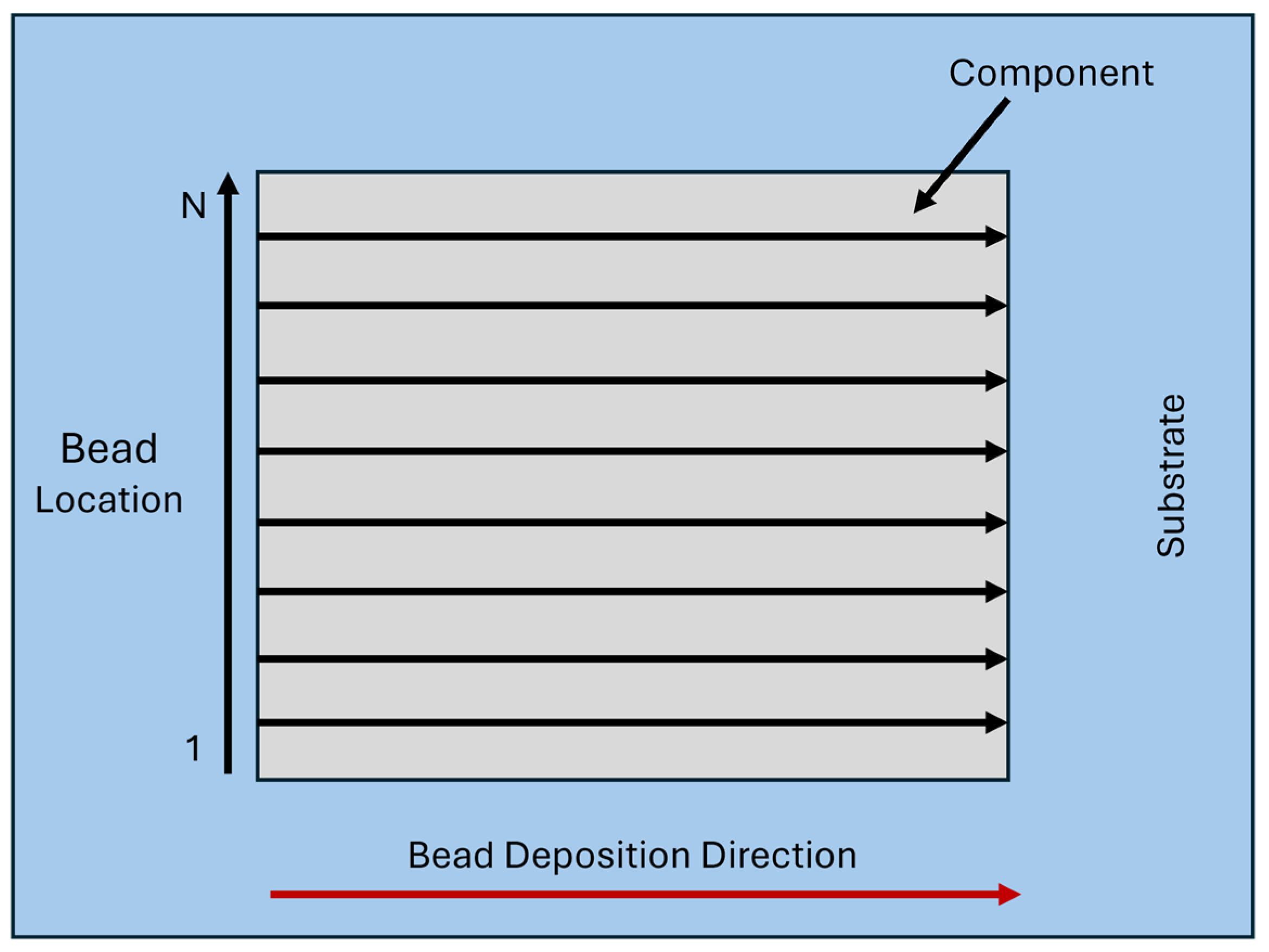
2.2. Modeling and Path Planning

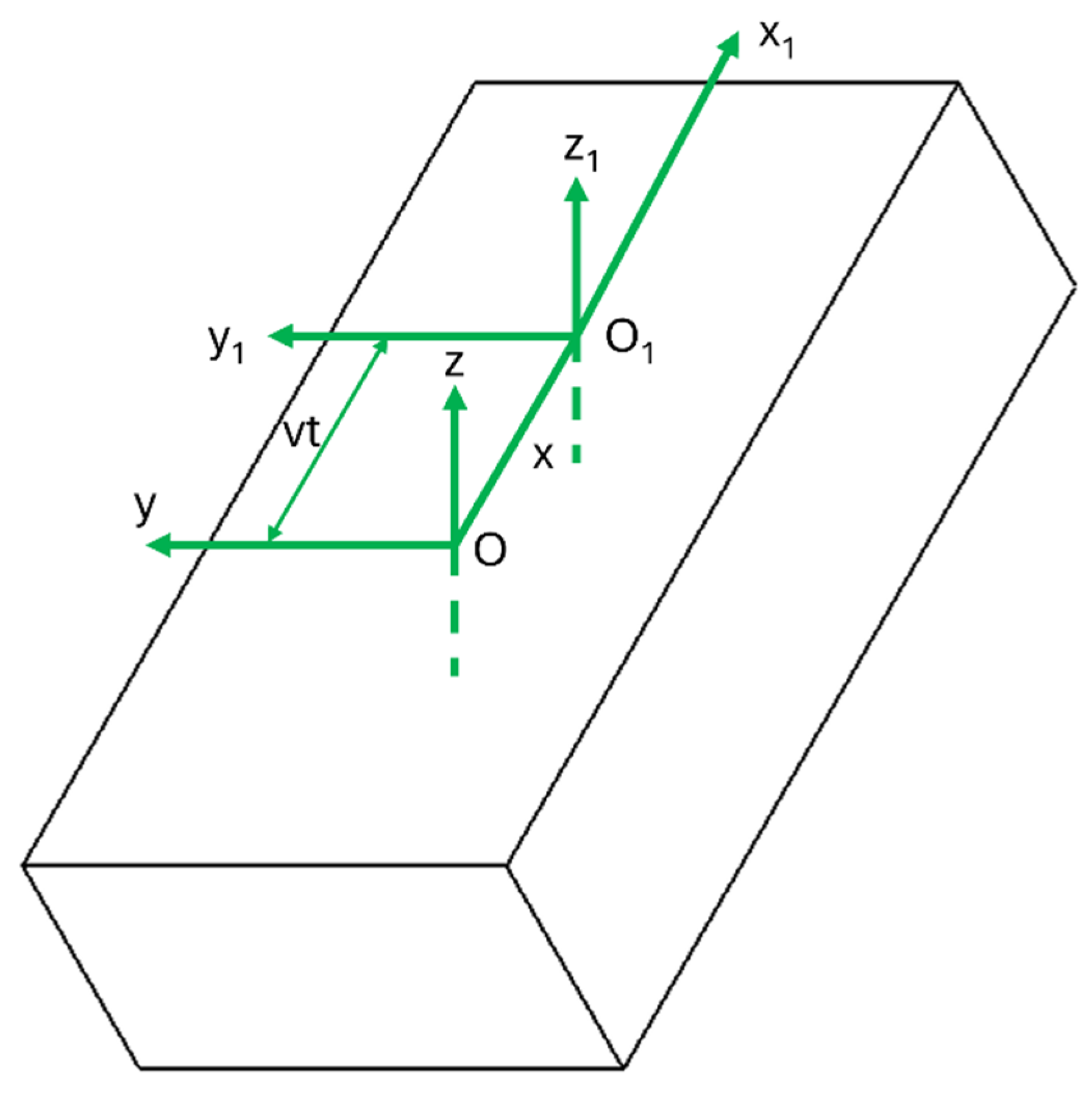
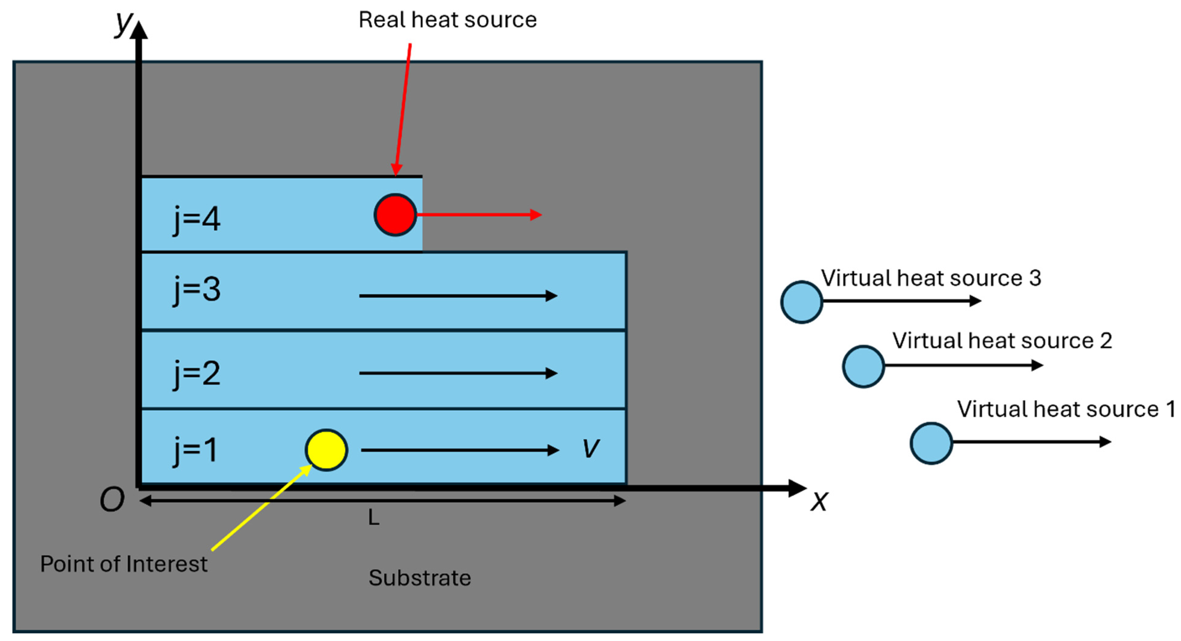
2.2.1. Analytic Model for Computing Temperature Field

For DED processes in general, including LHW-DED, interpass temperature, T_interpass, refers to the temperature at the deposition point. To calculate T_interpass, this study utilizes Rosenthal’s solution [34] to determine the temperature distribution resulting from previously deposited beads. In this approach, a virtual point heat source is assigned to each past bead, maintaining the same power, speed, and direction as the original physical laser heat source used to deposit that bead, even after the laser has moved to deposit subsequent beads. This assumes that the temperature distributions induced by the past beads are additive. As a result, T_interpass at any given point of interest can be calculated by superpositioning the temperature distributions from all previous beads.

In summary, the following two assumptions are made when computing the interpass temperature T_interpass prior to deposition:

Assumption 1: The conditions for applying Rosenthal’s solution are satisfied [34].

Assumption 2: The superposition principle holds for the temperature distributions induced by the steady-state point heat source associated with the deposition of each past bead.

The temperature calculation can be enhanced by providing more accurate characterization of the cooling effect that occurs after the laser heat source has completed deposition of the bead. The simulation of temperature evolution following the completion of a welding process was initially introduced by Rykalin [35]. After the real heat source is turned off following deposition, the temperature cooling process can be modeled by two distinct processes. One involves a virtual heat source representing the continuation of the original real heat source, and the other involves a virtual heat sink with an equal but negative power value. Considering time t and assuming that the laser is depositing the jth bead at time t, the temperature at a point of interest can be calculated by superpositioning the temperature contributions from the $(j-1$) virtual heat source and heat sink pairs representing the past (j − 1) beads, as well as the contribution of the real laser heat source depositing the $j$th bead,

$$T\left(x,y,z,t\right)=T_0+∆T_j^R+\sum _{i=1}^{j-1}∆T_i^V$$

(1)

where $T_0$ denotes the room temperature, $∆T_j^R$ represents the temperature contribution of the real laser heat source depositing the $j$th bead, and $∆T_i^V$ represents the temperature contribution from the virtual heat source and heat sink pair $i$.

Let $\left(x_j^R,y_j^R,z_j^R\right)$ denote the coordinates of the real heat source depositing the $j$th bead at time t, with laser power q_j and speed v_j. The temperature contribution $∆T_j^R$ is computed as [35]:

$$\begin{array}{c}∆T_j^R\left(x,y,z,t\right)={\displaystyle \frac{q_j}{2\pi k{R}_j}}{e}^{-{\displaystyle \frac{v_j\left({\xi }_j+R_j\right)}{2a}}}·\Gamma \left(v_j,R_j,t-t_j^0\right)\end{array}$$

(2)

with

$$\Gamma \left(v_j,R_j,t-t_j^0\right)={\displaystyle \frac{1}{2}}\left(A_{j}exp\left({\displaystyle \frac{v_j{R}_j}{a}}\right)+B_j\right)$$

(3)

and

$$A_j=1-erf\left({\displaystyle \frac{v_j\left(t-t_j^0\right)+R_j}{2\sqrt{a\left(t-t_j^0\right)}}}\right),B_j=1+erf\left({\displaystyle \frac{v_j\left(t-t_j^0\right)-R_j}{2\sqrt{a\left(t-t_j^0\right)}}}\right)$$

(4)

where ${\xi }_j$ = $x-x_j^R$, $R_j=\sqrt{{\xi }_j^2+{(y-y_j^R)}^2+{(z-z_j^R)}^2}$, $t_j^0$ denotes the time when the deposition of bead j begins, k represents the thermal conductivity, and a denotes the thermal diffusivity.

Similarly, let $\left(x_i^V,y_i^V,z_i^V\right)$ denote coordinates of the virtual heat source and heat sink pair i at the time t; then, the temperature contribution $∆T_i^V$ can be calculated as follows [35]:

$$\begin{array}{c}{∆T}_i^V\left(x,y,z,t\right)={\displaystyle \frac{q_i}{2\pi k{R}_i}}{e}^{-{\displaystyle \frac{v_i\left({\xi }_i+R_i\right)}{2a}}}·\Gamma \left(v_i,R_i,t-t_i^0\right)+{\displaystyle \frac{-q_i}{2\pi k{R}_i}}{e}^{-{\displaystyle \frac{v_i\left({\xi }_i+R_i\right)}{2a}}}\\ ·\Gamma \left(v_i,R_i,t-(t_i^0+{\displaystyle \frac{L}{v_i}})\right)\end{array}$$

(5)

where ${\xi }_i$ = $x-x_i^V$, $R_i=\sqrt{{\xi }_i^2+{(y-y_i^V)}^2+{(z-z_i^V)}^2}$, and L denotes the bead length. Derivation of the modified Rosenthal’s solution can be found in [35] and Appendix A.

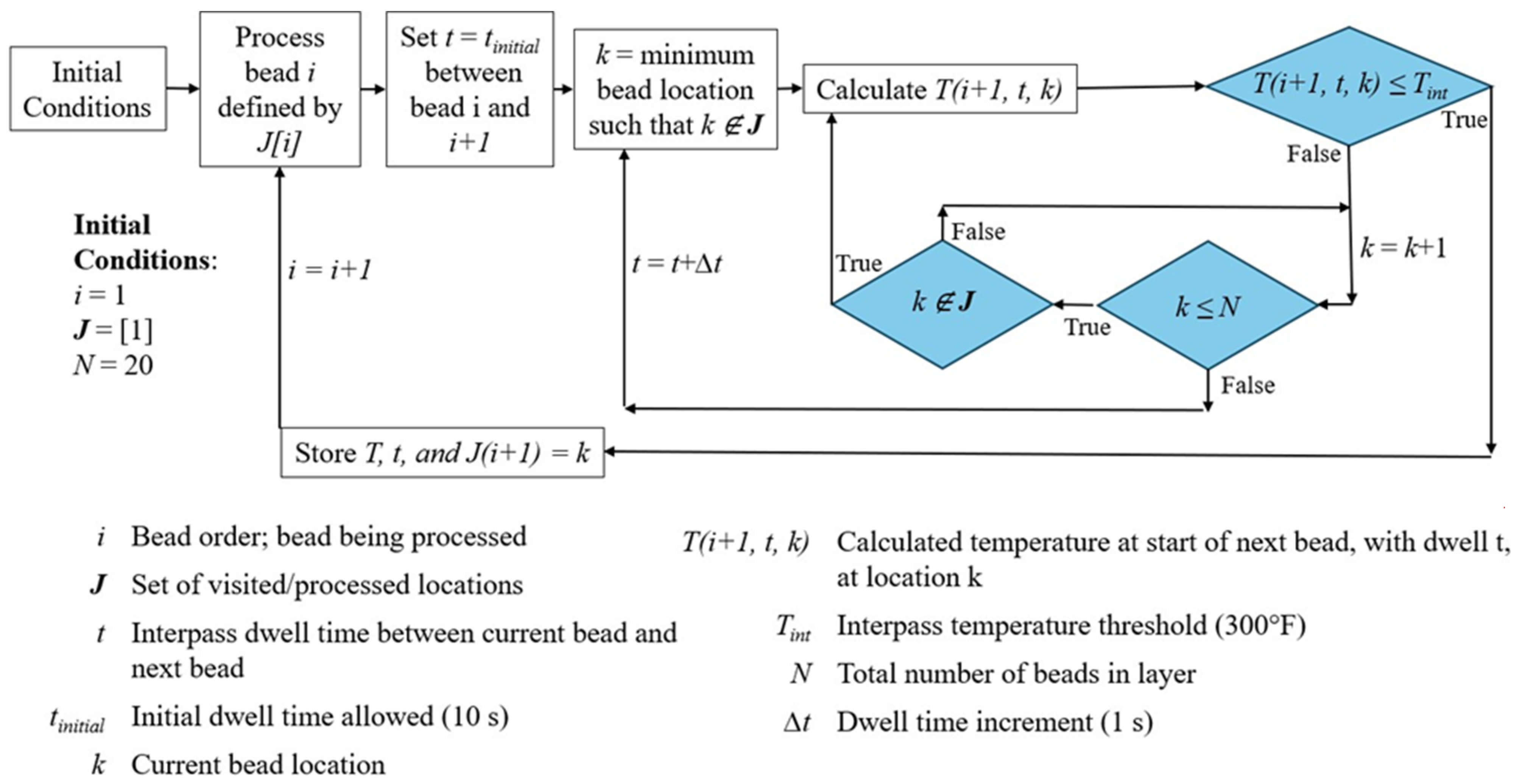
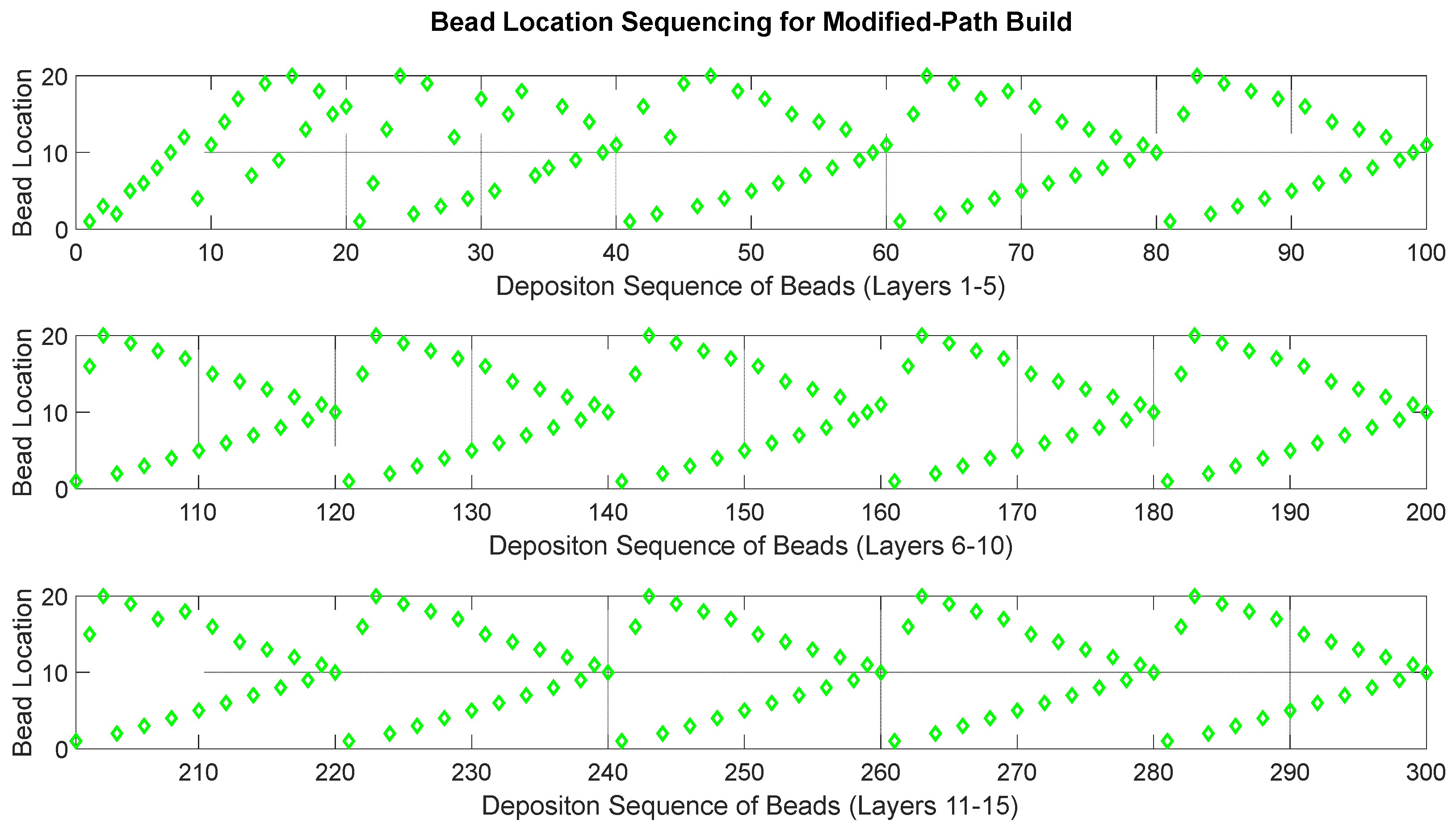
2.2.2. Algorithm for Path Planning

In this study, a greedy algorithm is developed for path planning based on the temperature prediction by the modified Rosenthal’s solution described in Section 2.2.1. The objective is to select an appropriate deposition path sequence so that the interpass temperature requirement can be met with minimal interpass dwell time, leading to reduced overall build time compared to the conventional sequential deposition path. Instead of conducting an exhaustive search over all possible scan path combinations, which is computationally prohibitive for large parts, this study uses a greedy algorithm to search for the next deposition bead, ensuring the interpass temperature requirement is met with minimal increase in the interpass dwell time. As a greedy algorithm, the choice for the next deposition bead by the algorithm is only optimal at the moment of decision, i.e., at the completion of depositing the current bead [36]. The greedy algorithm is iteratively applied after each deposited bead, using the thermal prediction strategy outlined in Section 2.2.1.

Consider a part consisting of N uni-directional beads in each layer, as shown in Figure 2. Each bead location ($i=1,2,\dots ,N$) refers to the physical location where each bead will be deposited in relation to the substrate. One conventional path planning method is to deposit the beads in a sequential manner from $i=1$ to $i=N$. The proposed greedy algorithm in this study is illustrated in Figure 3.

An initial interpass dwell time $t_{initial}$ is set to account for laser movement from the end of one bead to the start of the next bead. Next, the location of the next bead, k, is found by checking through all unprocessed bead locations in the current layer. The first available bead location, ranging from 1 to N, that satisfies the interpass temperature requirement, $T\le T_{int}$, is selected. The predicted interpass temperature T at any candidate bead location $k$ is calculated using the simplified thermal model given in Section 2.2.1. If temperatures at all remaining bead locations on the current layer are above the target interpass temperature, $T_{int}$, the dwell time is increased by $∆t$ and the process is repeated. This is iterated for every deposited bead in the current layer, and then the entire process is repeated for every layer of the part. The bead deposition sequence for the entire build is recorded. In this study, $t_{initial}$ is set to 10 s, and the increment for interpass dwell time is set to $∆t=1$ s, as smaller values increase computational load without significantly affecting the interpass temperature.

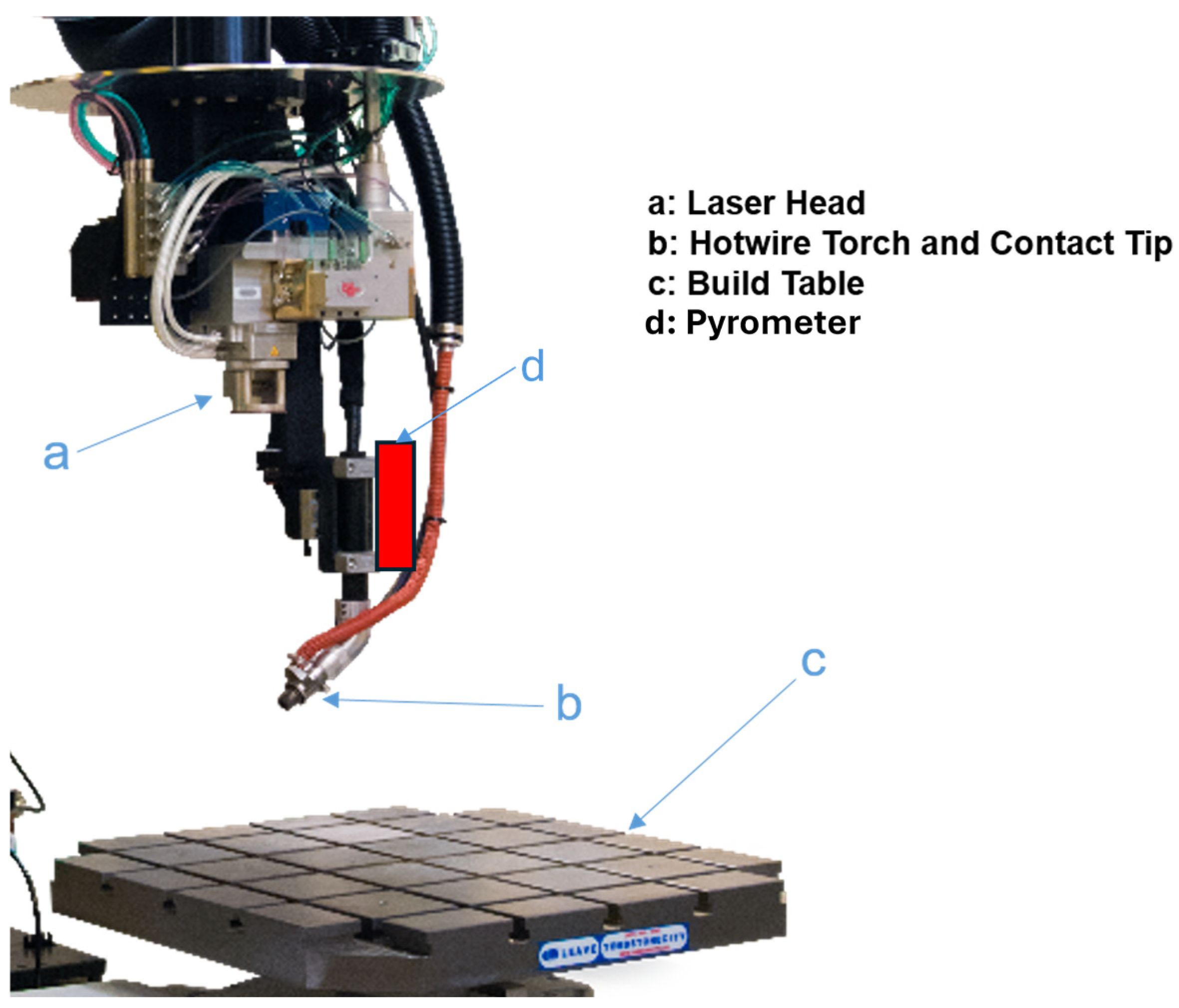
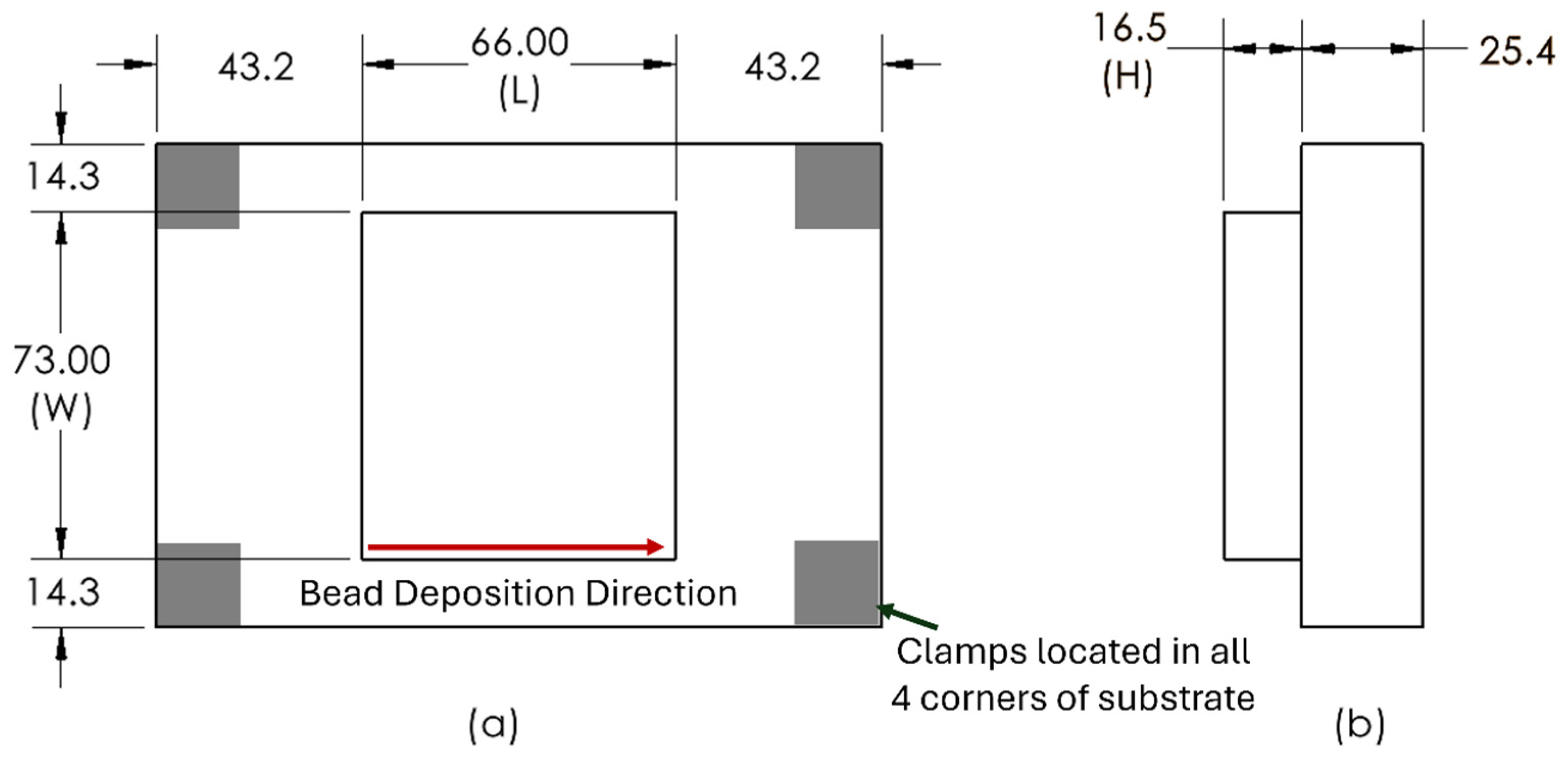
2.3. Experimental Setup

A series of ER100S-G wire-fed coupons, including the baseline (following the sequential deposition path) and modified-path builds (results from the greedy algorithm), are fabricated on HY80 steel substrates for comparison. Figure 4 shows the part and substrate dimensions. Each corner of the substrate is clamped, with a torque of 20.3 Nm, onto the positioner table.

Each sample comprises 15 layers, and each layer consists of 20 uni-directional beads, with a hatch spacing of 4.5 mm. After depositing each layer, the laser head is moved up in the z-direction by 1.1 mm to deposit the next layer. A laser power of 7.5 kW with an assumed efficiency of 60% [37] and a laser travel speed of 13 mm/s are used for deposition under an ambient temperature of 20 °C. All hot wire and laser parameters are listed in Table 1 and Table 2 in Section 2.1.

The in situ temperature measurements are performed using a water-cooled RayTek-GPS pyrometer (Raytek Corporation, Santa Cruz, CA, USA) with a measurement accuracy of ±1% or ±1 °C, whichever is greater. The pyrometer was calibrated before use in this study for temperature measurements. After depositing each bead, the pyrometer is positioned over the starting position of the next bead to obtain temperature measurements. The pyrometer is kept in this position until the measurements show a reading at or below the interpass temperature threshold of 149 °C (300 °F). The actual interpass dwell time required for the measured interlayer temperature to meet the threshold value is then recorded under each deposition path (baseline or modified).

As shown in Figure 5, the baseline build uses a sequential path scanning technique, where the laser deposits beads from 1 to 20 sequentially, from layer 1 to layer 15, with a total of 300 beads. For the modified-path samples, Figure 6 shows the bead sequencing selected by the greedy algorithm described in Section 2.2.2. These two deposition paths are applied to test coupons for comparison.

As shown in Figure 6, for the first few beads, there is little difference between the baseline and modified scan path as the entire part and substrate are still cool. As the heat in the part accumulates, the modified deposition path starts to diverge from the baseline. Essentially, the modified path starts to alternate between each side of the part, progressing from the outside cooler areas inward when the set of available bead locations decreases.

2.4. ER100S-G Wire

To produce high-quality components, the ER100S-G material requires that the interpass temperatures stay within 121–177 °C (250–350 °F) [23,24,25]. An interpass temperature of 149 °C (300 °F) is used as the threshold value in this study.

Table 3. ER100S-G chemical composition. Data from [38].

Composition (wt-%)	C	Mn	Si	Ni	Mo	Cr	S	P	V
ER100S-G	(0.05–0.06)	(1.63–1.69)	(0.46–0.50)	(1.88–1.96)	(0.43–0.45)	(0.04–0.06)	(0.002–0.005)	(0.005–0.009)	<0.01

lists the material composition specification of ER100S-G.

For simplicity, the constant material properties of the ER100S-G wire and substrate are used in the analytic thermal model to speed up the prediction of interpass temperatures. The thermo-mechanical properties of ER100S-G required for welding are not available in the literature. However, as ER100S-G is considered a filler metal in welding HY 80 [23,24], the material properties of HY 80 near the interpass temperature threshold are used in the thermal calculations (

Table 4. HY80 material properties near interpass temperature of 121–177 °C (250–350 °F). Data from [39].

Specific Heat	580 ${\displaystyle \frac{\mathrm{J}}{\mathrm{k}\mathrm{g}\mathrm{K}}}$
Density	7700 ${\displaystyle \frac{\mathrm{k}\mathrm{g}}{{\mathrm{m}}^3}}$
Thermal Conductivity	35 ${\displaystyle \frac{\mathrm{W}}{\mathrm{m}\mathrm{K}}}$

). While variations in material properties may introduce slight differences in the simulation results, the properties used in this study correspond to those of the base material, in which the ER100S-G wire is typically employed as a filler. As such, any resulting deviations are expected to be small. This assumption is supported by the results presented in Section 3.2, which show a prediction error of only 4.78% in build time.

2.5. Projecting Results to Larger Components

The samples used for experimental validations consist of 15 layers with 20 beads per layer, for a total of 300 beads. It is expected that the build time reduction will grow as the parts become larger. To account for this, we conduct simulations to evaluate the greedy algorithm in conjunction with the analytic thermal model, predicting build times for larger components by scaling up each dimension of the experimental samples five-times. These dimensions are varied independently to assess the effect of the modified deposition path on the simulated build time savings.

For each baseline case, the simulated interpass dwell time is computed using the modified Rosenthal’s solution in Section 2.2.1 until the temperature at the start of the next deposition drops below the required interpass temperature. Then, the simulated build times under the baseline and the modified deposition path are calculated by summing up all interpass dwell times and deposition times of all beads.

3. Results and Discussion

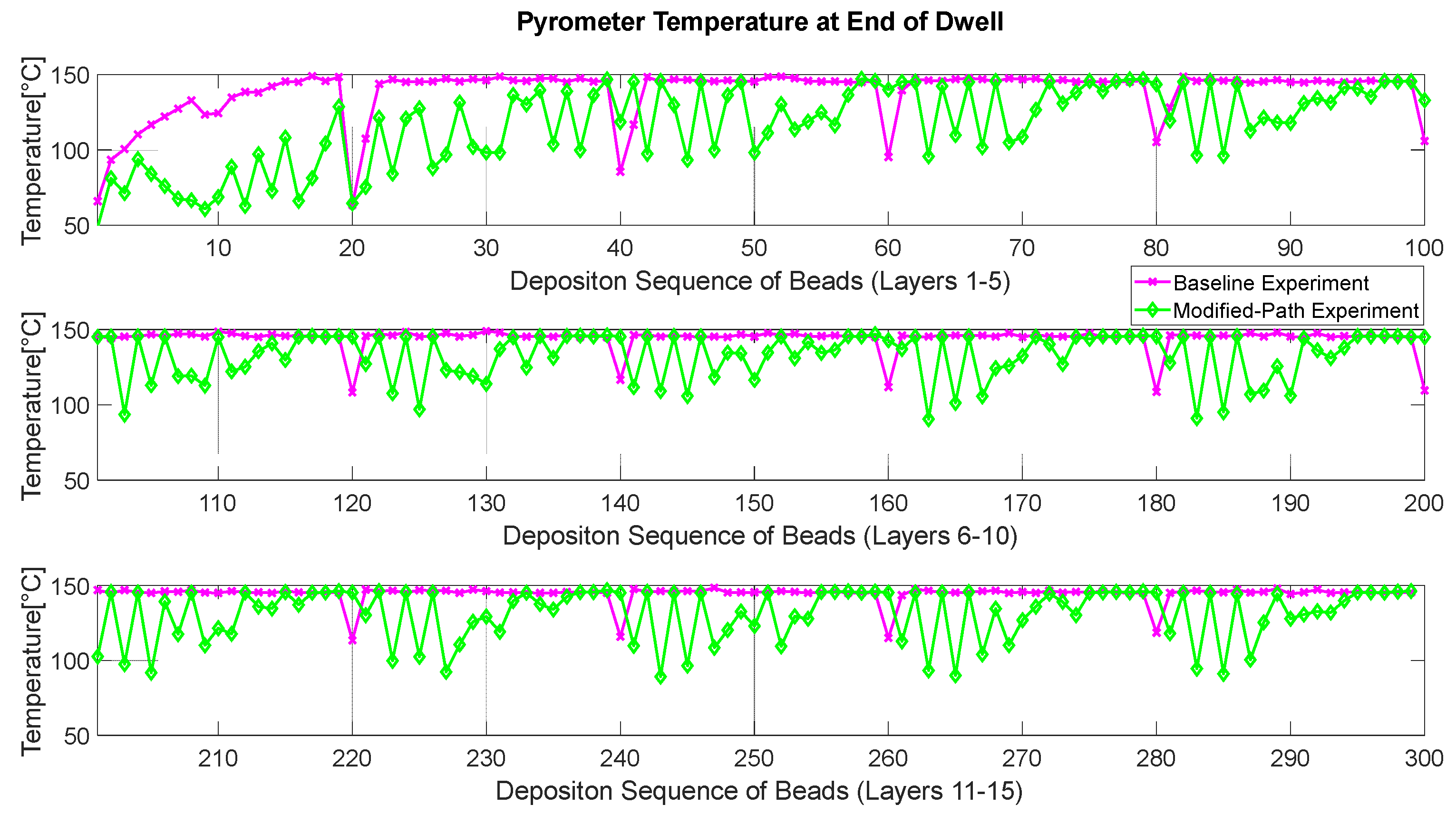
3.1. Measured Interpass Temperatures

We first verify that the interpass temperature requirement of all builds is satisfied. Figure 7 shows interpass temperatures measured by the pyrometer at the start of the next bead after the interpass dwell for both the baseline and modified-path experiments. Two experimental samples of the modified-path build were fabricated, and the results in all figures represent the average. It can be observed that all interpass temperatures for the experiments fall under the required temperature of 149 °C (300 °F).

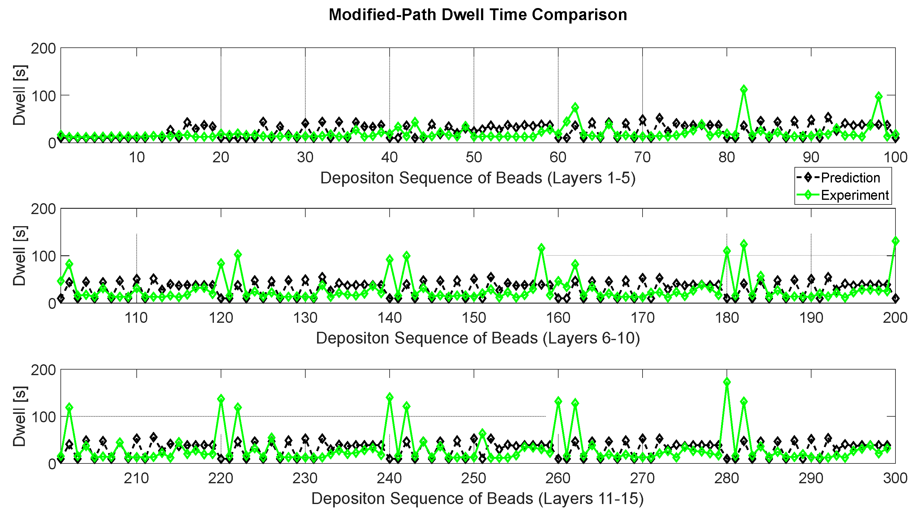
3.2. Predicted Interpass Dwell Time vs. Measurements

As illustrated in Section 2.2.2, the required interpass dwell times are computed along with the modified deposition path in the greedy algorithm. Figure 8 compares the predicted versus measured interpass dwell times for the experiment.

It can be observed that after layer 4, to meet the interpass temperature requirement, the actual interpass dwell times required at the very beginning and end of each layer are higher than the dwell times in the middle of that layer. This is due to heat buildup while processing the layer, which requires longer dwell times to cool the build. In addition, it is observed that the actual dwell times are higher than their corresponding predicted values at the beginning and end of each layer while slightly lower than their predicted values at the middle of each layer. The modified Rosenthal’s solution, which does not account for convection or radiation heat losses, predicts higher temperatures, leading to longer average dwell times in the middle of each layer. Furthermore, the modified Rosenthal’s solution in Section 2.2.1 does not account for the boundary conditions, leading to underestimating the interpass temperatures close to part edges and, thus, predicting lower interpass dwell times at these locations.

Figure 9 shows a comparison of the predicted versus measured cumulative time at the end of each layer under the modified-path scanning strategy. The cumulative time at the end of layer i is the sum of cumulative time at the end of layer (i − 1) plus the summation of interpass dwell times and deposition times within layer i. The prediction aligns with the measurements, though it slightly overestimates the total deposition time.

The predicted build time for the sample of 15 layers and 300 beads is 10,268 s, which is 4.78% higher than the actual sample-average build time of 9777 s. The small difference between the predicted and experimentally measured build time under the optimized deposition path indicates that, although the simplified thermal model in Section 2.2.1 is based on many assumptions and approximations, the resulting prediction on build time has a reasonable agreement with the experimental measurements.

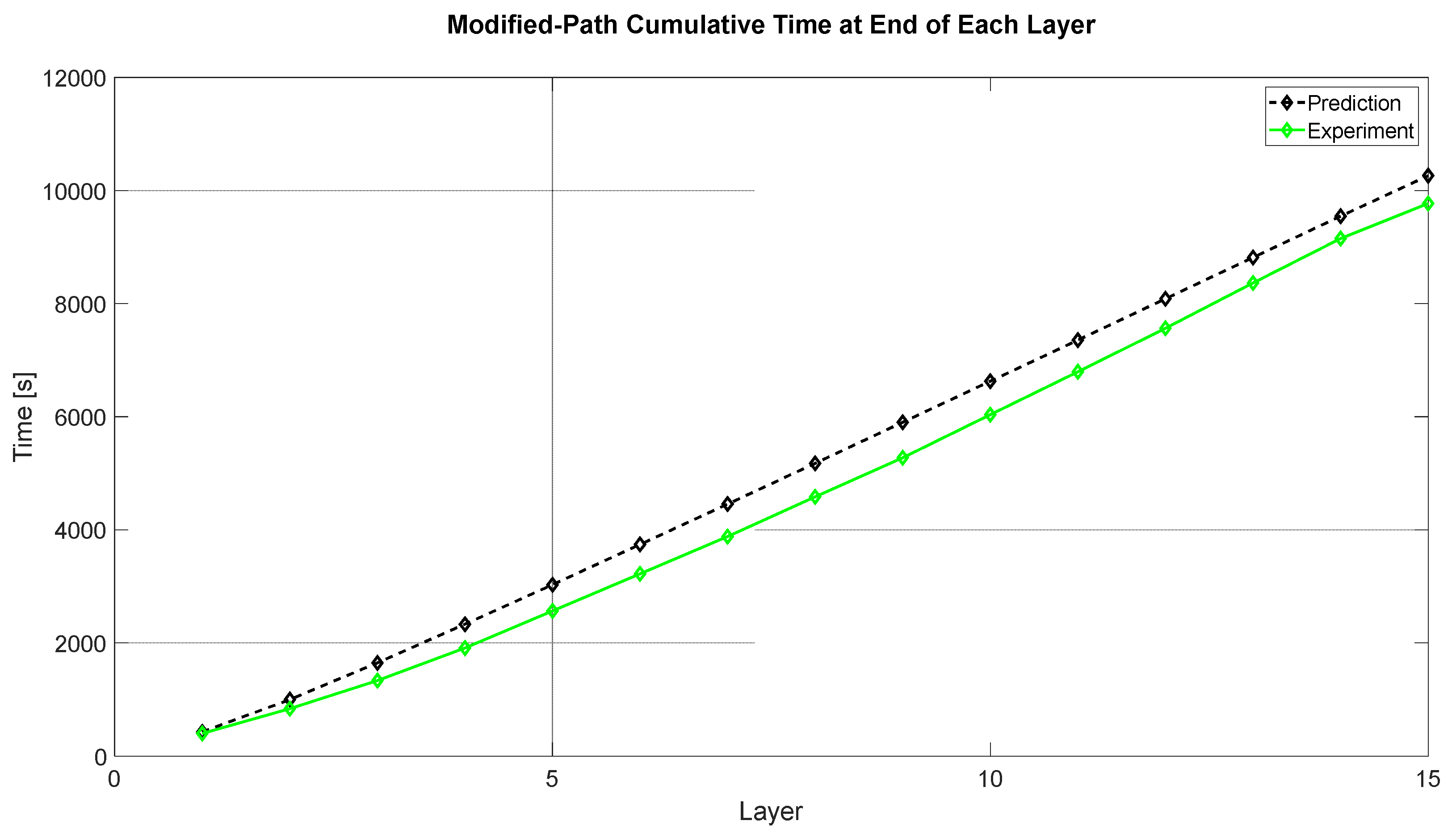
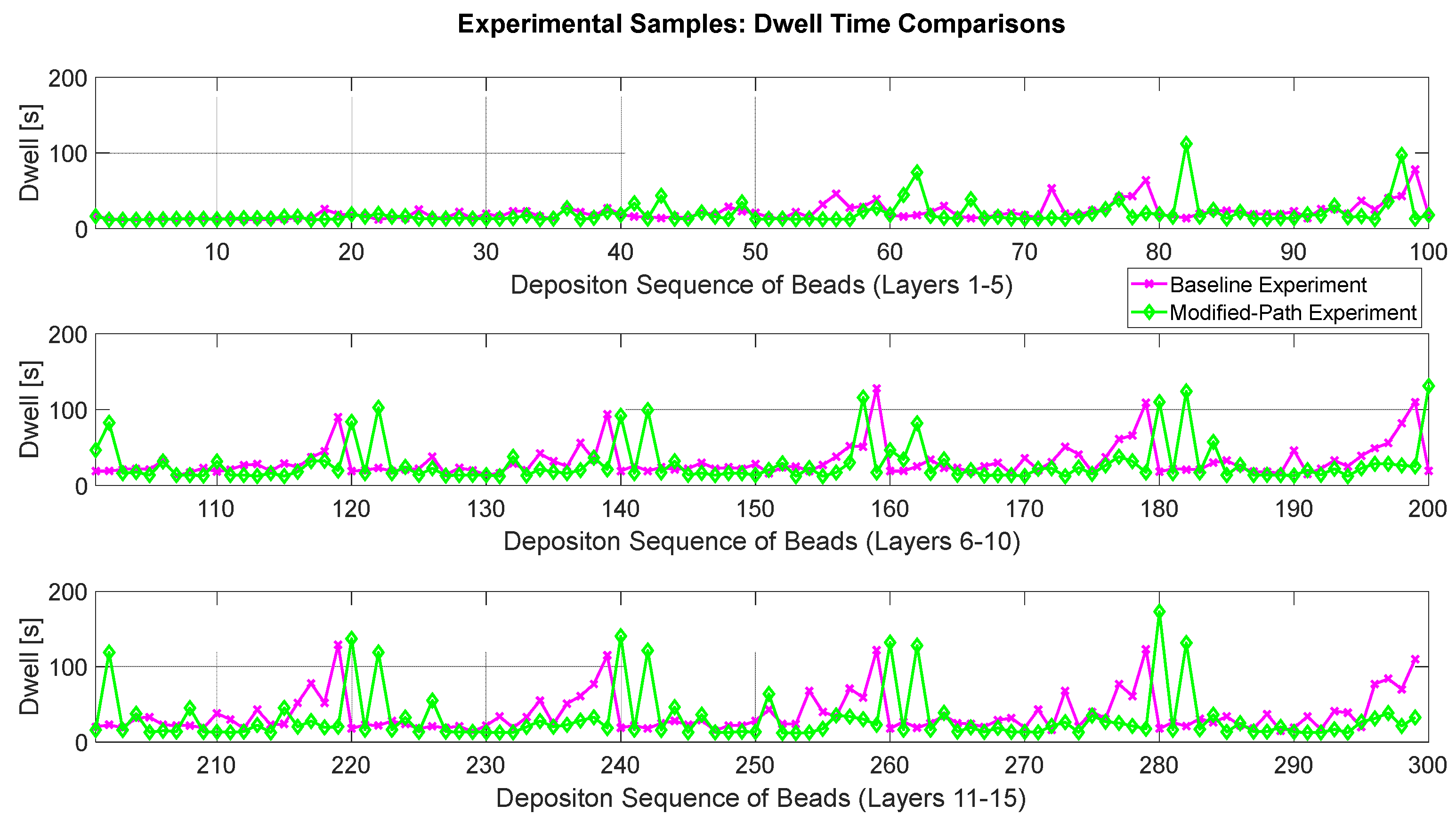
3.3. Build Time Reduction

To analyze the performance of the greedy algorithm, we next compare the baseline results to the modified-path results in terms of build time. Figure 10 shows a comparison of the measured interpass dwell times of the modified-path vs. baseline builds.

For the first few layers, there is not much difference between the baseline and modified path, as the entire part is still cool. For the first 10 beads of the first layer, the modified deposition path generated by the greedy algorithm closely follows the sequential depositional path, as shown in Figure 7 and Figure 8. With the increase in the layer number, the samples under the modified deposition path have lower interpass dwell times for most of the beads in a layer except for beads at the very start or end of each layer. This trend becomes more pronounced in the last few layers (layers 9–15).

Figure 11 shows a comparison of the cumulative time at the end of each layer of the baseline versus the modified-path samples. In the first five layers, as the entire part and substrate are still cool, there is a negligible difference in the cumulative time between the baseline and modified-path samples. As the layer count increases, the cumulative time of the baseline grows more quickly for the modified-path samples. The total build time for the baseline is 10,769 s, while the build time for the modified-path experiment is 9777 s, indicating a time reduction of 9.2% under the modified deposition path.

3.4. Predicted Build Time Reduction for Larger Components

As discussed in Section 2.4, the build time reduction is expected to grow as the parts become larger. Simulations were conducted to evaluate the thermal model in conjunction with the greedy algorithm for larger components. The evaluation cases and corresponding component dimensions are summarized in

Table 5. Component dimensions and predicted build times under baseline and modified-path strategies. The dimensions listed are in mm. Part No. 1 corresponds to the build dimensions of the experimental samples.

Part Number	Length [mm]	Width [mm]	Height [mm]	Predicted Build Time for Baseline [s]	Predicted Build Time for Modified Path [s]	Predicted Time Savings [%]	CPU Runtime [s]
1	66	92.5	16.5	11,849	10,268	13.3	75.2
2	330	92.5	16.5	24,492	22,982	6.2	173.9
3	66	452.5	16.5	43,616	26,178	40.0	234.2
4	330	452.5	16.5	93,817	66,776	28.8	2091.9
5	66	92.5	66	48,466	42,227	12.9	1050.8
6	330	92.5	66	106,398	101,026	5.0	2747.9
7	66	452.5	66	169,415	105,839	37.5	3011.6
8	330	452.5	66	383,990	284,358	25.9	40,787.0

. Part No. 1 in Table 5 represents the part dimensions of the experimental samples.

Table 5 shows that increasing the sample width by five-times (Part No. 3) is expected to reduce the deposition time by 40%. Because the beads are deposited along the direction of the part length, increasing the part width essentially increases the set of available deposition locations, allowing more freedom for path planning. In contrast, increasing the part length by only five-times (Part No. 2) is expected to reduce the deposition time by only 6.2%, while increasing the part height only (Part No. 5) is predicted to lead to a 12.9% reduction in build time.

The modified-path bead locations for Parts 1–4 (all have the same height) are shown in Figure 12, where only the first five layers are shown for clarity in the illustration. It is observed that only changing the length of the build results in small changes to the proposed bead locations in the modified-path build, while changing the width of the build results in vastly different path planning. This is because the component width offers a larger set of bead locations, providing more options for the path planning algorithm and reducing unnecessary back-and-forth movements. Increasing the length, however, does not create additional bead deposition locations, resulting in a minimal impact on the modified-path deposition.

The path planning algorithm in conjunction with the analytic thermal model was run on a computer with a peak RAM of 128 GB with ten cores and 3.7 GHz. Table 5 (last column) gives the CPU runtime for each predicted case. The computation cost increases as the part dimensions increase, with the largest increase corresponding to part height, i.e., the number of layers.

4. Conclusions

This study presents a path planning algorithm for DED AM that complies with interpass temperature requirements while reducing the total deposition time compared to the conventional sequential deposition path. The proposed approach utilizes a modified Rosenthal’s solution to evaluate the temperature as an input in a greedy algorithm, which then selects the optimal path with a minimal increase in the interpass dwell time. Experimental validation is conducted using a robotic LHW-DED of ER100S-G and employing in situ measurements of interpass temperature and interpass dwell time needed to satisfy the required interpass temperature. A calibrated pyrometer was used to obtain measurements. Samples were built with the sequential deposition path (baseline) and with the modified deposition path generated by the greedy algorithm. The results show that the prediction error for the total build time is less than 5% for the modified deposition path, demonstrating sufficient accuracy of the reduced-order model. In addition, the modified deposition path reduced the total build time by more than 9% compared to the baseline deposition path while still satisfying the interpass temperature requirement (less than or equal to 149 °C or 300 °F).

Though simulations, we show that the build time reduction can scale with increasing build size. For instance, a fivefold increase in the build width results in a simulated 40% reduction in the total build time. Future efforts will explore the incorporation of temperature-dependent properties to improve the accuracy of the thermal prediction model while addressing the associated increase in computational cost. Additional future work will evaluate the potential of this control strategy to reduce distortion by influencing the thermal history, optimizing path selection using thermal cost functions, and integrating process parameters such as laser power into the control framework.

References

1. Bambach, M.; Sizova, I.; Silze, F.; Schnick, M. Comparison of laser metal deposition of Inconel 718 from powder, hot and cold wire. Procedia CIRP 2018, 74, 206–209. [Google Scholar] [CrossRef]
2. Mao, Y.; Chen, H.; Xiong, J. Research progress in laser additive manufacturing of aluminum alloys: Microstructure, defect, and properties. J. Mater. Res. Technol. 2024, 30, 695–716. [Google Scholar] [CrossRef]
3. Wen, P.; Feng, Z.; Zheng, S. Formation quality optimization of laser hot wire cladding for repairing martensite precipitation hardening stainless steel. Opt. Laser. Technol. 2015, 65, 180–188. [Google Scholar] [CrossRef]
4. Wen, P.; Shan, J.; Zheng, S.; Wang, G. Control of wire transfer behaviors in hot wire laser welding. Int. J. Adv. Manuf. Technol. 2016, 83, 2091–2100. [Google Scholar] [CrossRef]
5. Liu, S.; Liu, W.; Kovacevic, R. Experimental investigation of laser hot-wire cladding. Proc. Inst. Mech. Eng. B J. Eng. Manuf. 2017, 231, 1007–1020. [Google Scholar] [CrossRef]
6. Liu, S.; Liu, W.; Harooni, M.; Ma, J.; Kovacevic, R. Real-time monitoring of laser hot-wire cladding of Inconel 625. Opt. Laser. Technol. 2014, 62, 124–134. [Google Scholar] [CrossRef]
7. Huang, Z.; Wang, G.; Wei, S.; Li, C.; Rong, Y. Process improvement in laser hot wire cladding for martensitic stainless steel based on the Taguchi method. Front. Mech. Eng. 2016, 11, 242–249. [Google Scholar] [CrossRef]
8. Kottman, M.; Zhang, S.; McGuffin-Cawley, J.; Denney, P.; Narayanan, B.K. Laser Hot Wire Process: A Novel Process for Near-Net Shape Fabrication for High-Throughput Applications. Miner. Met. Mater. Soc. 2015, 67, 622–628. [Google Scholar] [CrossRef]
9. Zhang, Z.; Kong, F.; Kovacevic, R. Laser hot-wire cladding of Co-Cr-W metal cored wire. Opt. Lasers. Eng. 2020, 128, 105998. [Google Scholar] [CrossRef]
10. Budde, L.; Biester, K.; Lammers, M.; Hermsdorf, J.; Kaierle, S.; Overmeyer, L. Influence of process parameters on single weld seam geometry and process stability in Laser Hot-Wire Cladding of AISI 52100. Adv. Ind. Manuf. Eng. 2023, 7, 100122. [Google Scholar] [CrossRef]
11. Stavropoulos, P.; Pastras, G.; Tzimanis, K.; Bourlesas, N. Addressing the challenge of process stability control in wire DED-LB/M process. CIRP Ann. 2024, 73, 129–132. [Google Scholar] [CrossRef]
12. Funderburk, R.S. The Importance of Interpass Temperature Key Concepts in Welding Engineering. Weld. Innov. 1998, XV, 31–32. [Google Scholar]
13. Wang, X.L.; Tsai, Y.T.; Yang, J.R.; Wang, Z.Q.; Li, X.C.; Shang, C.J.; Misra, R.D.K. Effect of interpass temperature on the micros tructure and mechanical properties of multi-pass weld metal in a 550-MPa-grade offshore engineering steel. Weld. World 2017, 61, 1155–1168. [Google Scholar] [CrossRef]
14. Wongpanya, P.; Boellinghaus, T.; Lothongkum, G.; Kannengiesser, T. Effects of Preheating and Interpass Temperature on Stresses in S 1100 QL Mult-Pass Butt-Welds 79 Welding in the World-Research Supplement. Weld. World 2008, 52, 79–92. [Google Scholar] [CrossRef]
15. Ramjaun, T.; Stone, H.J.; Karlsson, L.; Kelleher, J.; Moat, R.J.; Kornmeier, J.R.; Dalaei, K.; Bhadeshia, H.K.D.H. Effect of interpass temperature on residual stresses in multipass welds produced using low transformation temperature filler alloy. Sci. Technol. Weld. Join. 2014, 19, 44–51. [Google Scholar] [CrossRef]
16. Sirin, K.; Sirin, S.Y.; Kaluc, E. Influence of the interpass temperature on t8/5 and the mechanical properties of submerged arc welded pipe. J. Mater. Process. Technol. 2016, 238, 152–159. [Google Scholar] [CrossRef]
17. Geng, H.; Li, J.; Xiong, J.; Lin, X. Optimisation of interpass temperature and heat input for wire and arc additive manufacturing 5A06 aluminium alloy. Sci. Technol. Weld. Join. 2017, 22, 472–483. [Google Scholar] [CrossRef]
18. Ma, Y.; Cuiuri, D.; Shen, C.; Li, H.; Pan, Z. Effect of interpass temperature on in-situ alloying and additive manufacturing of titanium aluminides using gas tungsten arc welding. Addit. Manuf. 2015, 8, 71–77. [Google Scholar] [CrossRef]
19. Shen, C.; Pan, Z.; Cuiuri, D.; Ding, D.; Li, H. Influences of deposition current and interpass temperature to the Fe3Al-based iron aluminide fabricated using wire-arc additive manufacturing process. Int. J. Adv. Manuf. Technol. 2017, 88, 2009–2018. [Google Scholar] [CrossRef]
20. Derekar, K.; Lawrence, J.; Melton, G.; Addison, A.; Zhang, X.; Xu, L. Influence of Interpass Temperature on Wire Arc Additive Manufacturing (WAAM) of Aluminium Alloy Components. MATEC Web Conf. 2019, 269, 5001–5006. [Google Scholar] [CrossRef]
21. Poulain, P.; Wang, J.; Bouvier, S.; Williams, S.; Budnyk, S.; Gavrilovic-Wohlmuther, A. Impact of interpass temperature on the microstructure and mechanical properties of super duplex stainless steel in CW-GMA additive manufacturing. J. Manuf. Process. 2025, 146, 30–43. [Google Scholar] [CrossRef]
22. Ren, K.; Liu, N.; Zhang, W.; Chew, Y.; Zhang, Y.; Fuh, J.Y.; Bi, G. Laser power planning in directed energy deposition by deep reinforcement learning. Int. J. Adv. Manuf. Technol. 2024, 135, 4683–4694. [Google Scholar] [CrossRef]
23. Pinnacle Alloys. ER100S-G DATA SHEET. 2015, Volume 0117. Available online: http://www.pinnaclealloys.com/wp/wp-content/uploads/2015/11/Pinnacle-Alloys-ER100S-G-1.17.pdf (accessed on 29 January 2025).
24. Weldcote Metals. ERS100S-1. 2020, Volume 54. Available online: https://weldcotemetals.com/dataFiles/specs/tech100S-1.pdf (accessed on 29 January 2025).
25. American Welding Society (Committee on Filler Metals and Allied Materials). Specification for Low-Alloy Steel Electrodes and Rods for Gas Shielded Arc Welding, 5th ed.; Miami, F.L., Ed.; American Welding Society: Doral, FL, USA, 2022. [Google Scholar]
26. Antonysamy, A. Microstructure, Texture and Mechanical Property Evolution During Additive Manufacturing of Ti6Al4V Alloy for Aerospace Applications. Ph.D. Dissertation, University of Manchester, Manchester, UK, 2012. [Google Scholar]
27. Montevecchi, F.; Venturini, G.; Grossi, N.; Scippa, A.; Campatelli, G. Idle time selection for wire-arc additive manufacturing: A finite element-based technique. Addit. Manuf. 2018, 21, 479–486. [Google Scholar] [CrossRef]
28. Vázquez, L.; Rodríguez, N.; Rodríguez, I.; Alberdi, E.; Álvarez, P. Influence of interpass cooling conditions on microstructure and tensile properties of Ti-6Al-4V parts manufactured by WAAM. Weld. World 2020, 64, 1377–1388. [Google Scholar] [CrossRef]
29. Ren, K.; Chew, Y.; Fuh, J.Y.H.; Zhang, Y.F.; Bi, G.J. Thermo-mechanical analyses for optimized path planning in laser aided additive manufacturing processes. Mater. Des. 2019, 162, 80–93. [Google Scholar] [CrossRef]
30. He, C.; Wood, N.; Bugdayci, N.B.; Okwudire, C. Generalized SmartScan: An Intelligent LPBF Scan Sequence Optimization Approach for Reduced Residual Stress and Distortion in Three-Dimensional Part Geometries. J. Manuf. Sci. Eng. 2025, 147, 041001. [Google Scholar] [CrossRef]
31. Song, G.H.; Lee, C.M.; Kim, D.H. Investigation of path planning to reduce height errors of intersection parts in wire-arc additive manufacturing. Materials 2021, 14, 6477. [Google Scholar] [CrossRef]
32. Zhao, T.; Yan, Z.; Wang, L.; Pan, R.; Wang, X.; Liu, K.; Guo, K.; Hu, Q.; Chen, S. Hybrid path planning method based on skeleton contour partitioning for robotic additive manufacturing. Robot. Comput. Integr. Manuf. 2024, 85, 102633. [Google Scholar] [CrossRef]
33. Nguyen, L.; Buhl, J.; Bambach, M. Multi-bead overlapping models for tool path generation in wire-arc additive manufacturing processes. Procedia Manuf. 2020, 47, 1123–1128. [Google Scholar] [CrossRef]
34. Rosenthal, D. Mathematical Theory of Heat Distribution During Welding and Cutting. Weld. J. 1941, 20, 220–234. [Google Scholar]
35. Rykalin, N.N. Calculation of Heat Processes in Welding; Repositories of The University of Texas at Austin: Austin, TX, USA, 1960. [Google Scholar]
36. Cohen, H.; Eisenbud, D.; Singer, M. The Greedy Algorithm. In Graphs, Networks, and Algorithms; Springer: Berlin/Heidelberg, Germany, 2008; pp. 129–153. [Google Scholar]
37. Wu, S.S.Q.; Baker, B.W.; Rotter, M.D.; Rubenchik, A.M.; Wiechec, M.E.; Brown, Z.M.; Beach, R.J.; Matthews, M.J. Polarization effects associated with thermal processing of HY-80 structural steel using high-power laser diode array. Opt. Eng. 2017, 56, 124108. [Google Scholar] [CrossRef]
38. LINCOLN® ER100S-1. January 2022. Available online: www.lincolnelectric.com (accessed on 29 January 2025).
39. Baker, B.; McNelley, T.; Matthews, M.; Rotter, M.; Rubenchik, A.; Wu, S. Use of high-power diode laser arrays for pre- and post-weld heating during friction stir welding of steels. In Friction Stir Welding and Processing VIII; Springer International Publishing: Berlin/Heidelberg, Germany, 2016; pp. 21–36. [Google Scholar] [CrossRef]
40. Cao, Z.; Dong, P.; Brust, F. Fast thermal solution procedure for analyzing 3D multi-pass welded structures. Eng. Mater. Sci. 2000, 455, 12–21. [Google Scholar]
41. Perret, W.; Schwenk, C.; Rethmeier, M. Comparison of Analytical and Numerical Welding Temperature Field Calculation. Comput. Mater. Sci. 2010, 47, 1005–1015. [Google Scholar] [CrossRef]
42. Li, J.; Wang, Q.; Michaleris, P. An analytical computation of temperature field evolved in directed energy deposition. J. Manuf. Sci. Eng. Trans. ASME 2018, 140, 101004. [Google Scholar] [CrossRef]
43. Li, J.; Wang, Q.; Michaleris, P. Towards Computational Modeling of Temperature Field Evolution in Directed Energy Deposition Processes. 2018. Available online: http://asmedigitalcollection.asme.org/DSCC/proceedings-pdf/DSCC2018/51906/V002T23A001/2376748/v002t23a001-dscc2018-8973.pdf (accessed on 29 January 2025).
Figure 1. Laser hot wire additive manufacturing, with pyrometer mounted for in situ temperature measurement.
Metals 15 00570 g001
Figure 2. Bead locations (represented by black horizontal arrows) for single layer of fabricated component.
Metals 15 00570 g002
Figure 3. Flow chart of greedy algorithm used to select path planning, used in conjunction with modified Rosenthal’s solution developed in Section 2.2.1. Single layer shown, with the entire process being repeated for each layer in the build. Blue-diamond blocks in the flow chart are decision blocks where the process flow diverges based on a true/false condition.
Metals 15 00570 g003
Figure 4. Component and substrate dimensions. All measurements are in mm. (a) Top view; (b) side view.
Metals 15 00570 g004
Figure 5. Baseline bead sequencing (represented by pink markers), where bead locations follow the definition given in Figure 2.
Metals 15 00570 g005
Figure 6. Modified bead sequencing (represented by green diamond markers), where bead locations are shown in Figure 2.
Metals 15 00570 g006
Figure 7. Measured interpass temperature before deposition of the next bead for both the baseline and modified-path experiments (15 layers consisting of 300 beads).
Metals 15 00570 g007
Figure 8. Interpass dwell time under the modified deposition path: prediction versus experimental measurements. The modified bead deposition sequence is given in Figure 6. Each layer has 20 beads, and the entire build consists of 15 layers and 300 beads.
Metals 15 00570 g008
Figure 9. Cumulative time (including both dwell time and deposition time) at the end of each layer deposition under the modified deposition path: prediction vs. experimental measurements. Each sample consists of 15 layers and a total of 300 beads. The cumulative time at the end of layer 15 is the total build time of the sample.
Metals 15 00570 g009
Figure 10. Dwell time comparison for experimental samples of baseline and modified path.
Metals 15 00570 g010
Figure 11. Comparison of cumulative build time at the end of each layer under the baseline deposition path versus under the modified deposition path.
Metals 15 00570 g011
Figure 12. Modified-path bead locations (represented by black markers) for changing component dimensions. These modified paths show the first five layers for Parts 1–4 shown in Table 5.
Metals 15 00570 g012