Article

Estimation of Activity and Molar Excess Gibbs Energy of Binary Liquid Alloys Pb-Sn, Al-Sn and In-Zn from the Partial Radial Distribution Function Simulated by Ab Initio Molecular Dynamics

1
Faculty of Metallurgical and Energy Engineering, Kunming University of Science and Technology, Kunming 650093, China
2
National Engineering Research Center of Vacuum Metallurgy, Kunming University of Science and Technology, Kunming 650093, China
3
Key Laboratory for Nonferrous Vacuum Metallurgy of Yunnan Province, Kunming University of Science and Technology, Kunming 650093, China
4
State Key Laboratory of Complex Nonferrous Metal Resources Clean Utilization, Kunming University of Science and Technology, Kunming 650093, China
*
Author to whom correspondence should be addressed.
Metals 2024, 14(1), 102; https://doi.org/10.3390/met14010102
Submission received: 14 December 2023 / Revised: 8 January 2024 / Accepted: 12 January 2024 / Published: 15 January 2024
(This article belongs to the Special Issue Thermodynamic Assessment of Alloy Systems)

Abstract

:
For the present, it is difficult to obtain thermodynamic data for binary liquid alloys by experimental measurements. In this study, the molecular dynamics processes of the binary liquid alloys Pb50-Sn50, Al50-Sn50, and In50-Zn50 were simulated by using the ab initio molecular dynamics (AIMD) principle, and their partial radial distribution functions (PRDF) were obtained at different simulation steps. Combined with the relevant binary parameters of the Molecular Interaction Volume Model (MIVM), Regular Solution Model (RSM), Wilson Model, and Non-Random Two-Liquid (NRTL) models. The integral terms containing the PRDF were computed using the graphical integration method to obtain the parameters of these models, thus estimating their activity and molar excess Gibbs energy. The total average relative deviations (ARD) of the activity and molar excess Gibbs energy estimates of the four models for the binary liquid alloys Pb50-Sn50, Al50-Sn50, and In50-Zn50 at full concentration when the PRDF is obtained by the symmetry method are MIVM: 21.59% and 59.35%; RSM: 21.63% and 60.27%; Wilson: 24.27% and 86.7%; NRTL: 23.9% and 83.24%. When the PRDF is obtained by the asymmetric method: MIVM: 22.86% and 68.08%; RSM: 32.84% and 68.66%; Wilson: 25.14% and 82.75%; NRTL: 24.49% and 85.74%. This indicates that the estimation performance of the MIVM model is superior to the other three models, and the symmetric method performs better than the asymmetric method. The present study also derives and verifies the feasibility of Sommer’s equation for estimating the molar excess Gibbs energy and activity of binary liquid alloy systems in the Miedema model by using different equations of enthalpy of mixing versus excess entropy given by Tanaka, Ding, and Sommer. The total ARD of Tanaka, Ding, and Sommer’s relational equations in the Miedema model for estimating the activities and molar excess Gibbs energies of the binary liquid alloys Pb-Sn, Al-Sn, and In-Zn are 3.07% and 8.92%, 6.09% and 17.1%, and 4.1% and 14.77%. The results indicate that the estimation performance of the Miedema model is superior to the other four models.

1. Introduction

The thermodynamic parameters of solutions are fundamental data for the development of new processes, process optimization, and theoretical research in many fields. The study of the thermodynamic properties of solutions is essential for metallurgical preparation or the development of new materials. Among them, binary liquid alloys are characterized by simple structure and easy processing, which are widely used in aerospace, automotive, marine, and other fields [1]. Due to the complexity and accuracy limitations of actual high temperature experiments, in many cases, the experimental measurement process is difficult and the thermodynamic data results obtained are not accurate [2,3]. Therefore, it is worthwhile to seek an accurate, convenient, and reasonable method to simulate the experimental part of thermodynamic research. Since most of the actual solutions in thermodynamic experiments are non-ideal solutions, a modified concentration (activity) instead of the actual concentration must be considered to accurately analyze the thermodynamic behavior of the solution when simulating and calculating the thermodynamic parameters [4,5]. Therefore, the activity becomes one of the important research topics in the field of thermodynamic properties, and the molar excess Gibbs energy of the alloy can also be used as a more intuitive comparison and reference for the value of the alloy activity as well as the change of the alloy activity.
Until now, scientists have proposed many methods for calculating activity coefficients, such as the regular solution model (RSM) proposed by Hilderande [6,7] in 1929 and Wilson [8] in 1964, who postulated that interactions between molecules depended mainly on the “local concentration” which could be expressed as a volume fraction, and proposed the Wilson equation. The Non-Random Two-Liquid (NRTL) Model equation proposed by Renon and Prausnitz in 1968 is based on the semiempirical equation for the concept of localized concentration [9]. Miedema et al. developed a semiempirical theoretical model in 1973. Miedema et al. extended the metacellular model used by Wigner–Seitz in the theoretical description of pure metals to binary alloys and developed an empirical model after the gradual improvement ofthe Miedema model [10,11]. Tao [12] in 2000, based on statistical thermodynamics and fluid phase equilibrium theory, derived a new expression for the regular coordination partition function of liquids and their mixtures. Tao put forward the concept of local coordination number of molecules in liquid mixtures and its expression, thus establishing a new model for the thermodynamics of liquid mixtures that is the Molecular Interaction Volume Model, abbreviated as MIVM, and the above models have been widely used.
Ab initio molecular dynamics (AIMD), also known as first-principles molecular dynamics, has the basic idea of taking the electronic structure of molecules and interatomic interactions as the basis of calculations and calculating the structure and properties of materials through molecular dynamics simulations [13,14]. AIMD calculation methods have a wide range of applications, which can be used to study the structure, thermodynamic properties, kinetic properties, and electronic structure of a variety of materials [15].
Based on the predictive activity models of various binary alloy systems and the principle of AIMD, this paper uses Materials Studio software (Materials Studio 7.0-2020) to construct a binary alloy metal molecular model [16]. Next, Vienna ab initio simulation package (VASP) software (VASP-5.4.1.) is used to simulate molecular dynamics processes to obtain the thermodynamic data required for the binary liquid alloy system, and the partial radial distribution function (g(r)) is obtained by Visual Merchandising (VMD) software (VMD-1.9.4a53) [17,18,19,20]. Then, the parameters required for the MIVM, RSM, Wilson, and NRTL models are obtained by calculating the potential energy function. Two methods (the PRDF is obtained by the asymmetry method and the PRDF is obtained by the symmetry method) were used to estimate the activity and molar excess Gibbs energy of liquid mixtures of three binary positive deviation systems, Pb50 Sn50, Al50 Sn50, and In50 Zn50. Selection of binary liquid alloys with 50 percent monometallic concentration have a low melting point, good fluidity, easy processing, and low cost. Another task is to estimate the molar excess Gibbs energy and activity of the three systems in the Miedema model using three different relation equations between mixing enthalpy and excess entropy given by Tanaka [21], Ding [22], and Sommer [23,24], and to compare the estimation effects of each model and the two methods.

2. Methods and Steps of Simulation Calculation

2.1. Obtaining the Partial Radial Distribution Function by AIMD

In this work, the simulation uses the AIMD principle. Firstly, the molecular configuration of the alloy cells was established in the Materials Studio simulation software using the Packing method [16]. A total of 118 atoms consisting of 59 Pb atoms and 59 Sn atoms; 126 atoms consisting of 63 Al atoms and 63 Sn atoms; and 122 atoms consisting of 61 In atoms and 61 Zn atoms were simulated by placing them into square cubic boxes with side lengths of 15.5 Å, 15 Å, and 14 Å, respectively. The densities of the three systems of Pb0.5-Sn0.5, Al0.5-Sn0.5, and In0.5-Zn0.5 were 8.632 g/cm3 [25], 4.53 g/cm3 [26], and 6.665 g/cm3, respectively [27]. Next, AIMD simulations based on density functional theory (DFT) were performed using the VASP software [17]. The exchange-correlation function employed the Perdew–Burke–Ernzerhof (PBE) function, which is based on the generalized gradient approximation (GGA) [18]. Ultrasoft pseudopotentials [19] were used. The cutoff energy is chosen to be 1.3 times higher than the maximum cutoff energy provided in the pseudopotential files [17], and the calculation accuracy was chosen to be 10−4 eV/Å for the electron step and 10−3 eV/Å for the ion step. In simulating the kinetics, the simulation temperatures were set to 1050 K, 973 K, and 730 K, respectively, with the NVT system [20] synthesized using a Nosé–Hoover thermostat for temperature control [28]. The time step was 3 fs and the maximum number of steps for the ion motion was 5000 (15 ps). The K-point is set to the Gamma point [17]. Subsequently, the trajectory file XDATCAR was obtained as an output of the VASP kinetic simulation calculations, which includes the atomic coordinate information output at certain step intervals (i.e., all the atomic coordinate information of the 5000 steps of the performed calculations). Subsequent import into the VMD software allows the direct generation of g(r) images and g(r) coordinate data required for stepwise calculations [29].

2.2. Obtaining the First Peak of the Partial Radial Distribution Function

The partial radial distribution function is a function that describes the distribution state of matter and is used to describe the distribution of particles in space. It is defined as the product of the probability of a particle appearing on the unit sphere around a point in space and the density of the particle distribution on the sphere. The partial radial distribution function is an important manifestation of orderliness in the liquid alloy system. The typical partial radial distribution function is shown in Figure 1 [30,31]. Function in the origin of the coordinates near the existence of a clear peak, the first peak can be expressed and the central atom has interaction around the atom distribution changes [32].
In this paper, r0: represents the abscissa of the starting point of non-zero values; r1: denotes the position of the first valley of the function gij(r); rm: is the position of the first peak of the function gij(r); the following gij(r) = gji(r), gii(r), gjj(r) denotes the partial radial distribution function. In this paper, the way of describing the partial radial distribution function is divided into two kinds: one is the partial radial distribution function in the r0~rm region of the integral value of the symmetric treatment to obtain the method called symmetric method; one is to directly select the integral value of the r0~r1 region of the partial radial distribution function of the method called asymmetric method. The following gives the three systems of all the g(r) images as well as all of the key points of the data in the following Figure 2, Figure 3 and Figure 4 and Table 1, Table 2 and Table 3:

2.3. Average Pair Potential Energy Functions for Binary Liquid Alloys

The interaction potential function of molecular pairs is an important element in the study of the structure of matter and plays a decisive role in the thermodynamic properties of matter. The unknown parameters in the molar excess Gibbs energy thermodynamic model contain potential energy information. The partial radial distribution function is the result of the dynamic equilibrium of molecules under the action of the potential energy function [33].
According to the equation for the intermolecular pair potential energy as a function of radial distribution in a highly dilute pure gas [34]:
g ( r ) = exp [ ε ( r ) / k T ]
k is the Boltzmann constant 1.38 × 10⁻²³ J/K and T is the temperature. Assume that this equation can be approximated for i-j binary liquid alloys in order to calculate their interatomic pair potential functions. According to the probability density distribution function and the expectation principle, the expressions for the molecular pair potentials, εii, εjj, and εij of the binary liquid alloy can be obtained as [35,36]:
ε i i k T = r 0 r 1 ε i i r g i i ( r ) r 0 r 1 4 π g i i ( r ) r 2 d r d V = r 0 r 1 ln g i i ( r ) g i i ( r ) r 2 d r r 0 r 1 g i i ( r ) r 2 d r
ε i j k T = r 0 r 1 ln g i j ( r ) g i j ( r ) r 2 d r r 0 r 1 g i j ( r ) r 2 d r             ε j j k T = r 0 r 1 ln g j j ( r ) g j j ( r ) r 2 d r r 0 r 1 g j j ( r ) r 2 d r ,
Thus, under the condition that g(r) is known, then the values of εii, εjj, and εij = εji can be calculated from Equations (2) and (3).

3. Thermodynamic Model

3.1. Molecular Interaction Volume Model (MIVM)

The MIVM possesses characteristics such as inclusivity, diffusion stability, and thermodynamic consistency. The model satisfies the Gibbs–Duhem equation [37], so it can also be used to describe the thermodynamic properties of partially mutually soluble systems. Tao used statistical thermodynamics in the derivation process to obtain configurational partition functions that include both volume and energy terms. The model is suitable for different temperature system transformations and has a wide range of applications with relatively mature physical significance.
For the i-j binary alloy system MIVM the molar excess Gibbs energy is expressed as [12]:
G m E R T = x i ln V m i x i V m i + x j V m j B j i + x j ln V m j x j V m j + x i V m i B i j x i x j 2 Z i B j i ln B j i x i + x j B j i + Z j B i j ln B i j x j + x i B i j
The molar excess Gibbs energy (GmE) measures the overall energy change, and fluid phase equilibrium studies also require knowledge of the component activities (a). The expression for the activity coefficient of component i is [12]:
ln γ i = ln V m i x i V m i + x j V m j B j i + x j ( V m j B j i x i V m i + x j V m j B j i V m i B i j x j V m j + x i V m i B i j ) x j 2 2 Z i B j i 2 ln B j i ( x i + x j B j i ) 2 + Z j B i j ln B i j ( x j + x i B i j ) 2
γi, γj are the activity coefficients of compositions i, j, a i = γ i x i   a j = γ j x j are the respective activities. Where R is the ideal gas constant of 8.314 J/(K.mol). T is the absolute temperature. Vmi, Vmj denote the molar volume of group elements i, j at the temperature of the system to be solved, respectively. xi, xj denote the local mole fractions of the group elements i, j, and Zi, Zj denote the first coordination numbers of pure substances i, j. Bij and Bji are the parameters of molecular pair energy interactions, define Bij, Bji [12]:
B i j = exp ε i j ε j j k T B j i = exp ε j i ε i i k T

3.2. Regular Solution Model (RSM)

The RSM was proposed by Hildebrand in 1929 [6,7]. This model assumes that the mixture enthalpy of the solution is non-zero, while the mixture entropy is equal to that of an ideal solution. In other words, this model considers the interactions between solvent molecules but neglects the influence of volume.
For the i-j binary alloy system RSM the molar excess Gibbs energy is expressed as [6,7]:
G m E R T = w k T x i x j
The expression for the activity coefficient of component i is [6,7]:
ln γ i = w k T x j 2
where w is the interaction parameter. The w k T expression obtained from Guggenheim’s lattice-like theory is used here [38]:
w k T = Z ε i j k T 1 2 ε i i k T + ε j j k T
Z is the average coordination number. For i-j binary liquid mixtures, the empirical formula for the local coordination number can be replaced by the expression containing the partial radial distribution function given by Hill [34]:
Z i i = x i ρ 0 4 π 0 r 2 g i j ( r ) d r             Z i j = x j ρ 0 4 π 0 r 2 g i j ( r ) d r Z j j = x j ρ 0 4 π 0 r 2 g j j ( r ) d r             Z j i = x i ρ 0 4 π 0 r 2 g j i ( r ) d r
ρ0 denotes the corresponding mean density for the corresponding alloy composition. Dorini gives the expression for the average coordination number Z based on the local coordination number of the liquid alloy used here [39]:
Z = x i ( Z i i + Z i j ) + x j ( Z j i + Z j j )

3.3. Wilson Model

The Wilson model was proposed by Wilson in 1964 [8]. Wilson used the ratio of the Boltzmann distribution to define the “local concentration”, in which the local volume fraction was defined. The disadvantage is that it cannot be used in systems where the liquid phase is partially miscible. For the i-j binary alloy system Wilson Model the molar excess Gibbs energy is expressed as [8]:
G m E R T = x i ln x i + A j i x j x j ln x j + A i j x i
The expression for the activity coefficient of component i is [8]:
ln γ i = ln x i + A j i x j + x j A j i x i + A j i x j A i j x j + A i j x i
where, the parameters Aij and Aji are defined as [8]:
A i j = V i V j exp ε i j ε j j k T A j i = V j V i exp ε i j ε i i k T

3.4. Non-Random Two-Liquid Model (NRTL)

The NRTL model was proposed by Renon and Prausnitz in 1968 [9]. This model was derived by combining a local composition equation, based on the non-random assumption, with a potential energy expression for liquid mixtures from the two-liquid theory. It overcomes the disadvantage that Wilson’s equation cannot be used for systems in which the liquid phase is partially miscible. This model is often considered the most balanced model in the organic field in terms of simplicity, accuracy, and rationality. Their molar excess Gibbs energy expression [9]:
G m E R T = x i x j τ j i exp α τ j i x i + x j exp α τ j i + τ i j exp α τ i j x j + x i exp α τ i j
The expression for the activity coefficient of component i is [9]:
ln γ i = x j 2 τ j i exp 2 α i j τ j i 2 x i + x j exp ( α i j τ j i ) 2 + τ i j exp 2 α i j τ i j x j + x i exp ( α i j τ i j ) 2
where, the model parameters τij and τji are defined as [9]:
τ i j = ε i j ε j j k T τ j i = ε j i ε i i k T
The meaning of α is related to the stochasticity of the mixtures, and the value ranges from 0.2 to 0.47, in this paper, we take 0.3; αij = αji, τij, τji can be expressed as the pair potential.

3.5. Miedema Model

The Miedema model is a semi-empirical theoretical model developed by Miedema in 1973 [10,11]. This model assumes that the Wigner–Seitz cell theory can be extended from pure metals to binary alloys, and they believe that the concept of cells in alloys is still valid. The Miedema model generation heat calculation is an important achievement in alloying theory in recent years, with wide practical application. The heat of generation of any binary alloy other than O, S, Se, and Te can be calculated by using the basic properties of the components. The relationship between the partial molar excess free energy G i E ¯ of component i and its activity coefficient in a binary alloy system consisting of component i and component j are expressed as:
G i E ¯ = R T ln γ i
The partial molar excess free energy of component i  G i ¯ and the Gibbs excess free energy of the i-j binary alloy system are related by:
G i E ¯ = G i j E + ( 1 + x i ) G i j E x i
In the binary system i-j, the molar excess Gibbs energy G i j E and excess entropy S i j E and the enthalpy change of Δ H i j are related by:
G i j E = Δ H i j T S i j E
T is the absolute temperature, in binary system alloys, the heat of generation can be obtained from the Miedema model, and the heat of generation in the formation of liquid solution or solid solution is derived as [10,11]:
Δ H i j = f i j x i 1 + u i x j ϕ i ϕ j x j 1 + u j x i ϕ j ϕ i x i V i 2 / 3 1 + u i x j ϕ i ϕ j + x j V j 2 / 3 1 + u j x i ϕ j ϕ i
f i j = 2 p V i 2 / 3 V j 2 / 3 q / p n w s i 1 / 3 n w s j 1 / 3 2 ϕ i ϕ j 2 a r / p n w s 1 / 3 i 1 + n w s 1 / 3 j 1
In Equations (21) and (22), xi and xj are the molar fractions of i and j, respectively; Vi and Vj are the molar volumes of group elements i and j, respectively; n w s i and n w s j are the electron densities of group elements i and j, respectively; ϕ i and ϕ j are the electronegativities of group elements i and j; p, q, µi, µj, b, r/p are constants and p/q = 9.4 for all alloys;

3.5.1. Relationship between Enthalpy of Mixing and Excess Entropy as Defined by Tanaka

Kubaschewiski and Alcock [40] examined the relationship between the enthalpy of mixing and excess entropy of binary alloys and concluded that there was an approximately linear relationship. After more careful study, Tanaka concluded that the ratio coefficient of S i j E and Δ H i j is related to the melting point of pure metals, which can be given by the relation [21]:
S i j E = Δ H i j 1 T m i + 1 T m j 14
Tmi and Tmj are monometallic melting points, the same applies below. Order:
β = 1 T 1 T m i + 1 T m j 14
Then one can obtain:
G i j E = β i j Δ H i j
Combined with the Miedema model Equations (21) and (22), the relationship between the activity coefficients of i as a function of component xi is obtained:
ln γ i = 1 R T β i j Δ H i j 1 + x j 1 x i 1 x j u i ϕ i ϕ j 1 + u i x j ϕ i ϕ j + u j ϕ j ϕ i 1 + u j x i ϕ j ϕ i V i 2 / 3 1 + u i 1 2 x i ϕ i ϕ j + V j 2 / 3 1 + u j 1 2 x i ϕ j ϕ i x i V i 2 / 3 1 + u i x j ϕ i ϕ j + x j V j 2 / 3 1 + u j x i ϕ j ϕ i

3.5.2. Relationship between Enthalpy of Mixing and Excess Entropy as Defined by Ding

Ding Xueyong gives different empirical constants based on S i j   E and Δ H i j relationship of [22]:
S i j E = 0.1 × Δ H i j 1 / T m i + ( 1 / T m j )
Order:
α i j = 1 0.1 T 1 / T m i + 1 / T m j
Then it is available:
G i j E = α i j Δ H i j
Next, in combined with the Miedema model Equations (21) and (22), the relationship between the activity coefficients of i as a function of component xi is obtained:
ln γ i = 1 R T α i j Δ H i j 1 + x j 1 x i 1 x j u i ϕ i ϕ j 1 + u i x j ϕ i ϕ j + u j ϕ j ϕ i 1 + u j x i ϕ j ϕ i V i 2 / 3 1 + u i 1 2 x i ϕ i ϕ j + V j 2 / 3 1 + u j 1 2 x i ϕ j ϕ i x i V i 2 / 3 1 + u i x j ϕ i ϕ j + x j V j 2 / 3 1 + u j x i ϕ j ϕ i

3.5.3. Relationship between Enthalpy of Mixing and Excess Entropy as Defined by Sommer

For the relationship between the enthalpy of mixing and excess entropy, Sommer, Germany, gave the following new expression based on the formula of V.T. Witusiewicz [41] in combination with binary system alloys [23,24]:
S i j E = Ω Δ H T + x i x j R P T
Among them [23,24]:
Ω = 1 2 π T ¯ m T ¯ b + 1
P T = 1 2 + 4 T ¯ m 3 T + 2 l n T T ¯ b T ¯ m
Tbi and Tbj are monometallic boiling points, respectively. T ¯ m = ( T m i + T m j ) / 2 ; T ¯ b = ( T b i + T b j ) / 2 , e is a natural constant.
Combining Equations (18), (19) and (29), ln γ i can be expressed as:
ln γ i = α i j H i j R T + α i j ( 1 + x i ) Δ H i j x i R T
Associative formulations (30) and (34) are available for the Miedema model:
Δ H i j x i = Δ H i j ( 1 x i 1 + x i ) 1 x i 1 1 x i μ i ( φ i φ j ) 1 + μ i ( 1 x i ) ( φ i φ j ) + μ i ( φ j φ i ) 1 + μ j x i ( φ j φ i ) V i 2 / 3 1 + μ i ( 1 2 x i ) ( φ i φ j ) + V j 2 / 3 1 + μ j ( 1 2 x i ) ( φ j φ i ) x i V i 2 / 3 1 + μ i x j ( φ i φ j ) + x j V j 2 / 3 1 + μ j x i ( φ j φ i )
The Sommer enthalpy change and entropy change relation combining Equations (18)–(20), (31)–(33) and (35) can ultimately lead to the derivation of expressions for the molar excess Gibbs energy and activity:
G i j E = ( 1 Ω ) Δ H i j x i ( 1 x i ) T Ω R P T
ln γ i = ( 1 Ω ) Δ H i j x i ( 1 x i ) T Ω R P T R T + ( 1 + x i ) ( 1 Ω ) Δ H i j x i ( 1 2 x i ) T Ω R P T R T = ( 1 Ω ) Δ H i j x i ( 1 x i ) T Ω R P T R T + ( 1 x i ) ( 1 Ω ) Δ H i j 1 x i 1 1 x i μ i ( φ i φ j ) 1 + μ i ( 1 x i ) ( φ i φ j ) + μ i ( φ j φ i ) 1 + μ j x i ( φ j φ i ) V i 2 / 3 1 + μ i ( 1 2 x i ) ( φ i φ j ) + V j 2 / 3 1 + μ j ( 1 2 x i ) ( φ j φ i ) x i V i 2 / 3 1 + μ i x j ( φ i φ j ) + x j V j 2 / 3 1 + μ j x i ( φ j φ i ) ( 1 + x i ) ( 1 2 x i ) T Ω R P T R T
For the Miedema model parameters are shown in Table 4. where the r/p value is only relevant for transition metal and non-transition metal alloys, and for two non-transition metals the p value is 10.6.

4. Results and Discussion

4.1. Parameters of Four Models

The expressions (2) and (3) for the average atom pair potential of the binary liquid alloy containing g(r) are substituted into the model parameter expressions (6), (9), (14), and (17) for MIVM, RSM, Wilson, and NRTL, respectively, and the values of the integral terms are calculated by using the graphical integration method with trapezoidal integration as the basic principle [43]. This method divides the integration region into several small trapezoids and sums their areas to obtain the integral value. Obviously, this method is different from the mathematical form of L-PPDF fitted with the Gaussian function by Chunlong Wang et al. [31], which depends on the fitting parameters u and v. Therefore, in this work, no fitting parameters are introduced in the process of solving each model parameter.
The parameter values of each model are calculated by using the asymmetric method and the symmetric method, as shown in Table 5. For the parameters of the symmetry method, the table presents the data calculated by multiplying by two the integral values of r0~rm in the selected g(r).
In order to visualize the difference between the fitted values and the experimental values more intuitive, the standard deviation SD and the average relative deviation ARD of the calculated results are denoted as:
SD = a e s t a exp 2 N ,   ARD = 1 N a e s t a exp a exp × 100 %
aest is the estimated value of activity and aexp [43,44,45] is the experimental value of activity.
SD = G m E e s t G m E exp 2 N ,   ARD = 1 N G m E e s t G m E exp G m E exp × 100 %
GmE(est) is the estimated value of the molar excess Gibbs energy and GmE(exp) [44,45,46] is the experimental value of the molar excess Gibbs energy.

4.2. Miedema Model Estimation of Molar Excess Gibbs Energy and Activity

The Miedema model is an empirical theoretical model. The molar excess Gibbs energy and activity of a binary alloy system can be estimated by the Miedema formula in combination with the basic properties of the group elements and the relevant parameters, simply by knowing the equation of the corresponding enthalpy of mixing of the alloy system in relation to the excess entropy. The experimental values of full concentration molar excess Gibbs energy (GEm), activity (a) of Pb-Sn, Al-Sn, and In-Zn alloys under the Miedema model are given below with the comparison and deviation of the calculated values in Table 6, Table 7 and Table 8 and Figure 5, Figure 6 and Figure 7.
Figure 5 and Table 6 show that for Pb-Sn alloys Tanaka Ding, and Sommer’s improved mixing enthalpy versus excess entropy relationship equation in the Miedema model to estimate the activity effect ARD is less than 10%. However, since the experimental values of the activity of Pb-Sn alloys are consistent with symmetry and are the effect of the presentation of very small deviations, so there is a possibility of chance in the estimation results
Figure 6 and Table 7 show that the estimation effect of the three methods for Al-Sn alloys is obvious. The activity ARD of the three methods is less than 5%, and the ARD of the estimated molar excess Gibbs energy is less than 10%, the estimation effect can be said to be accurate. The Sommer’s improved mixing enthalpy versus excess entropy relationship equation in the Miedema model has a better estimation effect.
Figure 7 and Table 8 show that for In-Zn alloys, Sommer’s formula is slightly less effective than the first two in estimating activity, with an ARD of 11.75%, while the ARD of the other two is less than 5%. This shows that all three methods give relatively good estimation results for different systems. The relation between the enthalpy of mixing and excess entropy given by Sommer is based on the application of the Miedema model to binary alloys in order to estimate the activity and molar excess Gibbs energy is reasonable and feasible. The total average relative deviations of Tanaka, Ding, and Sommer’s relational equations in the Miedema model for estimating the activities and molar excess Gibbs energies of the binary liquid alloys Pb-Sn, Al-Sn, and In-Zn are 3.07% and 8.92%, 6.09% and 17.1%, and 4.1% and 14.77%, respectively.

4.3. Estimation of the Molar Excess Gibbs Energy and Activity of Pb0.5-Sn0.5, Al0.5-Sn0.5, and In0.5-Zn0.5 Alloys at Full Concentration Using Partial Radial Distribution Functions

Table 9, Table 10, Table 11, Table 12, Table 13 and Table 14 show the results of stepwise calculations for the three systems using the symmetric and asymmetric methods in the four models, respectively. The ARD comparison images of all the activity distributions calculated for the three binary alloy systems under the asymmetric and symmetric methods are given, where the x-axis represents the four models. The two small bars for each model represent the asymmetric and symmetric methods under each model, the different colors of each bar represent the different ranges of the ARD values, and the scale of the bar is the number of data accounted for by the calculations of the nine sets of distributions, see Figure 8, Figure 9 and Figure 10.
Through Figure 8 it can be seen that the MIVM model in Pb-Sn alloy has the best overall estimation effect. The ARD less than 10% accounts for five of the nine sets of stepwise calculation data under the two methods. The symmetric method under the MIVM model has a better estimation performance. The RSM model has the second-best estimation performance, and the asymmetric method under the RSM model has a better estimation effect. The estimation effect of the Wilson and the NRTL models is poorer compared with the former two, there is no data of ARD less than 10%.
Through Figure 9 it can be seen in Al-Sn alloys in the RSM model the two methods ARD less than 20% of the data in the two methods under the nine groups of stepwise calculation data accounted for eight groups. Among the asymmetric methods, there were two groups with ARDs less than 10% and four groups with ARDs greater than 30%. The Figure 9 can only show that for the RSM model for Al-Sn alloys, the asymmetric method estimation of the precision of the higher degree of data is greater. The data with a high estimation degree of the MIVM model is second only to the RSM model and the asymmetric method is better under the MIVM model. Wilson model and NRTL model estimation of activity ARD has no data less than 20%, but there is more data with ARD between 20–30%, so it is necessary to calculate the average value to compare the estimation effect.
Figure 10 shows that the overall estimation effect of the MIVM model in In-Zn alloys is better. The ARD less than 30% accounts for seven of the nine sets of stepwise calculation data in the two methods, in which the symmetric method has a better estimation effect. The estimation effect of the RSM model is second to that of the MIVM model, in which the asymmetric method has a better estimation effect. The estimation effect of the Wilson model and the NRTL model is poorer compared to the former two, and the ARD does not have any data of less than 30%.
According to the data in Table 9, Table 10, Table 11, Table 12, Table 13 and Table 14, it can be calculated that the total average relative deviations of the activity estimates of the four models for the binary liquid alloys Pb50-Sn50, Al50-Sn50, and In50-Zn50 at the full concentrations. When the PRDF is obtained by the symmetry method are MIVM: 21.59%; RSM: 21.63%; Wilson: 24.27%; and NRTL: 23.9%. When the PRDF is obtained by the symmetry method are MIVM: 22.86%; RSM: 32.84%; Wilson: 25.14%; NRTL: 24.49%. Combined with Figure 8, Figure 9 and Figure 10, it can be concluded that the symmetric method of estimation is better than the asymmetric method in the three binary alloy systems. Among the four models, the MIVM model has a better estimation effect. The estimation results of the MIVM and RSM models fluctuate greatly with the number of steps, and the data distribution is not uniform. However, because of the high sensitivity of the estimation effect to the change in the number of steps, the estimation results are more consistent with the experimental values. The Wilson and NRTL models estimate the activity data with less variation as the number of steps changes, and the estimation effect is not good. The data obtained from Table 9, Table 10, Table 11, Table 12, Table 13 and Table 14 also reflect that not all systems are best estimated at 0–5000 steps (at full steps size).

5. Conclusions

For the calculation results and comparison of estimating the molar excess Gibbs energy and activity of binary alloys under the Miedema model using the relationship between mixing enthalpy and excess entropy given by Tanaka, Ding, and Sommer (the total ARD of the molar excess Gibbs energy and activity of the three binary liquid alloys under the Miedema model are Tanaka: 3.07% and 8.92%; Ding: 6.09% and 17.1%; Sommer: 4.1% and 14.77%). Preliminary validation of the rationality and feasibility of the Sommer relation for estimating the molar excess Gibbs energy and activity method for binary liquid alloys under the Miedema model. We hope that it can provide a reference for selecting appropriate models and methods to estimate thermodynamic data such as activity and excess Gibbs energy of binary liquid alloys.
Based on the AIMD principle, the kinetic process was simulated by VASP software to obtain the partial radial distribution function of the alloy at different step sizes, and the parameters of MIVM, RSM, Wilson, and NRTL models are calculated by the given pair of the potential energy function and two methods (asymmetric and symmetric methods) to estimate the molar excess Gibbs energy and activity of binary liquid alloys with good rationality and feasibility. The total ARD of the molar excess Gibbs energy and activity of the three binary liquid alloys at full concentration when the PRDF is obtained by the symmetry method are MIVM: 21.59% and 59.35%; RSM: 21.63% and 60.27%; Wilson: 24.27% and 86.7%; NRTL: 23.9% and 83.24%. When the PRDF is obtained by the asymmetric method: MIVM: 22.86% and 68.08%; RSM: 32.84% and 68.66%; Wilson: 25.14% and 82.75%; NRTL: 24.49% and 85.74%. These calculation results show that the ARD for the estimated activity is within reasonable limits, and it is reasonable and feasible to show that this given assumption can be used for the pair potential energy equation for binary liquid alloys. The results also show that the MIVM model performs better than the RSM, Wilson, and NRTL models, and the asymmetric method performs better than the symmetric method. Not all systems are best estimated at the simulation steps from 0 to 5000. This result hopefully provides a research direction for interested researchers (i.e., based on the AIMD principle, the PRDFs obtained from the simulation stepwise calculations by using the VASP software are best fit to the experimental values at which steps).

Author Contributions

Conceptualization, D.T., T.Z. and X.C.; Methodology, D.T.; Theoretical Guidance, D.T.; Review, D.T., X.C., Y.L. and J.H.; Writing—Original Draft, T.Z.; Writing—Review & Editing, T.Z.; Formal analysis, T.Z.; Software, T.Z.; Data Curation, T.Z.; Visualization, T.Z.; Resources, X.C.; Validation, Y.L. and J.H. All authors have read and agreed to the published version of the manuscript.
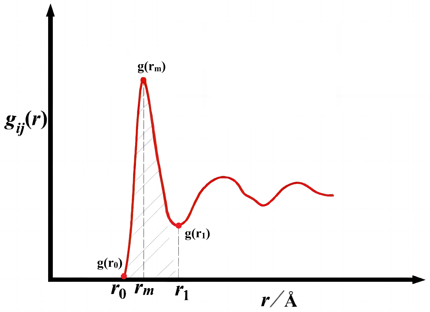
Funding

This work was financially supported by the National Natural Science Foundation of China under Grant (Grant No. 51464022).

Data Availability Statement

The raw data supporting the conclusions of this article will be made available by the authors on request.

Conflicts of Interest

The authors declare no conflict of interest.

References

  1. Chen, L.L.; Li, T.; Zhang, J.P.; Wang, Y.A.; Kong, L.X.; Xu, B.Q.; Yang, B.; Wu, M.Z. Modeling and measurement of vapor-liquid equilibrium of In–Pb and In–Pb–Sn alloy systems in vacuum distillation. Vacuum 2023, 207, 111556. [Google Scholar] [CrossRef]
  2. Wang, S.P.; Chen, L.L.; Xu, B.Q.; Jiang, W.L.; Kong, L.X.; Yang, B.; Xiong, H.; Qu, C.; Zhang, T.; Zhang, S.H.; et al. Theoretical calculation and experimental investigation on vacuum gasification separation of Ag-Cu-Au ternary alloy. J. Alloys Compd. 2023, 948, 169685. [Google Scholar] [CrossRef]
  3. Sun, G.Y.; Li, B.; Guo, H.J.; Yang, W.S.; Li, S.Y.; Guo, J. Thermodynamic Study of Energy Consumption and Carbon Dioxide Emission in Ironmaking Process of the Reduction of Iron Oxides by Carbon. Energies 2021, 14, 1999. [Google Scholar] [CrossRef]
  4. Zhu, Y.Q.; Chen, Z.J.; Zhang, H.M.; Ma, W.H.; Wu, J.J. The effect of Ni on Fe and Al impurities by MIVM model for the silicon production. Energy 2022, 254, 124459. [Google Scholar] [CrossRef]
  5. Zhao, X.; Cheng, S.X.; Koh, Y.P.; Kelly, B.D.; McKenna, G.B.; Simon, S.L. Prediction of the Synergistic Glass Transition Temperature of Coamorphous Molecular Glasses Using Activity Coefficient Models. Mol. Pharmaceut. 2021, 18, 3439–3451. [Google Scholar] [CrossRef]
  6. Hildebrande, J.H. The Regular Solution Model for Binary Alloys. Proc. Natl. Acad. Sci. USA 1927, 13, 267–272. [Google Scholar]
  7. Hildebrand, J.H. Solubility. VIII. Regular Solutions1. J. Am. Chem. Soc. 1929, 1, 66–80. [Google Scholar] [CrossRef]
  8. Wilson, G.M. Vapor-Liquid Equilibrium. Xi. A New Expression for the Excess Free Energy of Mixing. J. Am. Chem. Soc. 1964, 2, 127–130. [Google Scholar] [CrossRef]
  9. Renon, H.; Prausnitz, J.M. Local compositions in thermodynamic excess functions for liquid mixtures. Aiche J. 1968, 14, 135–144. [Google Scholar] [CrossRef]
  10. Miedema, A.R. The electronegativity parameter for transition metals: Heat of formation and charge transfer in alloys. J. Less Common Met. 1973, 32, 117–136. [Google Scholar] [CrossRef]
  11. Miedema, A.R.; Chtel, P.F.; Boer, F.R. Cohesion in alloys–fundamentals of a semi-empirical model. Phys. B+C 1980, 100, 1–28. [Google Scholar] [CrossRef]
  12. Tao, D.P. A New Model of Thermodynamics of Liquid Mixtures and its Application to Liquid Alloys. Thermochim. Acta 2000, 363, 105–113. [Google Scholar] [CrossRef]
  13. Zhang, D.; Tang, Y.Z.; Wang, S.; Lin, H.; He, Y. A study on the thermal resistance over metal–carbon nanotube interface by molecular dynamics simulation. Compos. Interfaces 2022, 29, 899–913. [Google Scholar] [CrossRef]
  14. Zhang, L.; Xiong, D.; Su, Z.; Li, J.; Yin, L.; Yao, Z.; Wang, G.; Zhang, L.; Zhang, H. Molecular dynamics simulation and experimental study of tin growth in SAC lead-free microsolder joints under thermo-mechanical-electrical coupling. Mater. Today Commun. 2022, 33, 104301. [Google Scholar] [CrossRef]
  15. Surmenev, R.; Grubova, I.Y.; Neyts, E.; Teresov, A.; Koval, N.; Epple, M.; Tyurin, A.; Pichugin, V.; Chaikina, M.; Surmeneva, M.; et al. Ab initio calculations and a scratch test study of RF-magnetron sputter deposited hydroxyapatite and silicon-containing hydroxyapatite coatings. Surf. Interfaces. 2020, 21, 100727. [Google Scholar] [CrossRef]
  16. Zhuang, C.Q.; Yue, H.; Zhang, H.J. Molecular Simulation Methods and Materials Studio Applications to Macromolecular Material. Plastics 2010, 39, 81–84. [Google Scholar] [CrossRef]
  17. Kresse, G.; Furthmüller, J. Efficient iterative schemes for ab initio total-energy calculations using a plane-wave basis set. Phys. Rev. B 1996, 54, 11169. [Google Scholar] [CrossRef]
  18. Boukideur, M.A.; Selhaoui, N.; Alaoui, F.C.; Poletaev, D.; Bouchta, H.; Achgar, K.; Aharoune, A. Thermodynamic assessment of the Ga–Lu system bythe combination of ab-initio calculations and the CALPHAD approach. Calphad 2022, 79, 102464. [Google Scholar] [CrossRef]
  19. Wang, S.Y.; Kramer, M.J.; Xu, M.; Wu, S.; Wang, C.Z. Experimental and ab initio molecular dynamics simulation studies of liquid Al60Cu40 alloy. Phys. Rev. B 2009, 79, 144205–144209. [Google Scholar] [CrossRef]
  20. Zhang, C.; Wei, Y.; Zhu, C. Structural and electronic properties of liquid InSb alloy: An ab initio molecular-dynamics simulation. Chem. Phys. Lett. 2005, 408, 348–353. [Google Scholar] [CrossRef]
  21. Tanaka, T.; Gokcen, N.A.; Spencer, P.J.; Morita, Z.I.; Tida, T. Evaluation of interaction parameters in dilute liquid ternary alloys by a solution model based on the free volume theory. Z. Für Metallkunde 1993, 84, 100–105. [Google Scholar] [CrossRef]
  22. Ding, X.; Wang, W.; Fan, P. Thermodynamic calculation for alloy systems. Metall. Mater. Trans. B 1999, 30, 271–277. [Google Scholar] [CrossRef]
  23. Witusiewicz, V.T.; Sommer, F. Estimation of the excess entropy of mixing and the excess heat capacity of liquid alloys. Cheminformation 2001, 312, 228–237. [Google Scholar] [CrossRef]
  24. Sommer, F.; Singh, R.N.; Witusiewicz, V. On the entropy of mixing. J. Alloys Compd. 2001, 325, 118–128. [Google Scholar] [CrossRef]
  25. Gąsior, W.; Moser, Z.; Pstruś, J. Density and surface tension of the Pb-Sn liquid alloys. J. Phase Equilib. Diff. 2001, 22, 20–25. [Google Scholar] [CrossRef]
  26. Chikova, O.; Vyukhin, V.; Tsepelev, V. Influence of Melt Superheating Treatment on the Cast Structure of Al–Sn Alloys. Russ. J. Non-Ferr. Met. 2021, 62, 286–292. [Google Scholar] [CrossRef]
  27. Pstruś, J.; Moser, Z.; Gąsior, W. Surface properties of liquid In–Zn alloys. Appl. Surf. Sci. 2011, 257, 3867–3871. [Google Scholar] [CrossRef]
  28. Sun, S.H.; Chen, X.M.; Zhang, F.X.; Yang, B. Ab Initio Molecular Dynamics Simulations of Cu under Vacuum and 473~1573K. Adv. Mater. Res. 2013, 690-693, 2699–2702. [Google Scholar] [CrossRef]
  29. Mackoy, T.; Kale, B.; Papka, M.E.; Wheeler, R.A. viewSq, a Visual Molecular Dynamics (VMD) module for calculating, analyzing, and visualizing X-ray and neutron structure factors from atomistic simulations. Comput. Phys. Commun. 2021, 264, 107881. [Google Scholar] [CrossRef]
  30. Debye, P.; Scherrer, P. Interferenzen an Regellos Orientierten Teilchen Im Rntgenlicht. I. Nachrichten von der Gesellschaft der Wissenschaften zu Göttingen, Mathematisch-Physikalische Klasse; Springer: Berlin, Germany, 1916; pp. 1–5. [Google Scholar]
  31. Zernike, F.; Prins, J. Die Beugung Von Röntgenstrahlen in Flüssigkeiten Als Effekt Der Molekülanordnung. Z. Für Phys. A Hadron. Nuclei. 1927, 6, 184–194. [Google Scholar] [CrossRef]
  32. Eisenstein, A.; Gingrich, N.S. The Diffraction of X-Rays by Argon in the Liquid, Vapor, and Critical Regions. Phys. Rev. 1942, 62, 261–270. [Google Scholar] [CrossRef]
  33. Allen, M.P.; Tildesley, D.J. Computer Simulation of Liquids; Oxford University Press: Oxford, UK, 1989; pp. 25–34. [Google Scholar]
  34. Hill, T.L. Statistical Mechanics: Principles and Selected Applications; Courier Corporation: Chelmsford, UK, 1957; pp. 185–209. [Google Scholar]
  35. Wang, C.; Chen, X.; Tao, D. Estimation of Component Activities and Molar Excess Gibbs Energy of 19 Binary Liquid Alloys from Partial Pair Distribution Functions in Literature. Metals 2023, 13, 996. [Google Scholar] [CrossRef]
  36. Feller, W. An Introduction to Probability Theory and its Applications; John Wiley & Sons: Hoboken, NJ, USA, 1950; pp. 220–222. [Google Scholar]
  37. Tao, D.P. The universal characteristics of a thermodynamic model to conform to the Gibbs-Duhem equation. Sci. Rep. 2016, 6, 35792. [Google Scholar] [CrossRef] [PubMed]
  38. Guggenheim, J.A. Application of Statistical Mechanics; Clarendon: Oxford, UK, 1966; p. 211. [Google Scholar]
  39. Dorini, T.T.; Eleno, L.T.F. Liquid Bi–Pb and Bi–Li alloys: Mining thermodynamic properties from ab-initio molecular dynamics calculations using thermodynamic models. Calphad 2019, 101687, 1–9. [Google Scholar] [CrossRef]
  40. Kubaschewski, O. Metallurgical thermochemistry. Int. Ser. Mater. Sci. Technol. 1977, 24, 478. [Google Scholar]
  41. Witusiewicz, V.T. Thermodynamics of liquid binary alloys of the 3d transition metals with metalloids: Generalization. J. Alloys Compd. 1995, 221, 74–85. [Google Scholar] [CrossRef]
  42. Gokcen, N.A. Statistical Thermodynamics of Alloys; Springer Science & Business Media: New York, NY, USA, 1986. [Google Scholar]
  43. Ramesh, B.; Preisser, N.; Michelic, S. Image Processing Procedure to Evaluate Inclusion Dissolution in a Slag Observed by High-Temperature Confocal Scanning Laser Microscopy. Metals 2022, 12, 531. [Google Scholar] [CrossRef]
  44. Franke, P.; Neuschütz, D. Binary Systems. Part 3. Binary Systems from Cs-K to Mg-Zr. In Thermodynamic Properties of Inorganic Materials of Landolt-Börnstein-Group IV Physical Chemistry; Springer: Berlin, Germany, 2005; Volume 19, pp. 1–3. [Google Scholar]
  45. Franke, P.; Neuschütz, D. Binary Systems. Part 4. Binary Systems from Mn-Mo to Y-Zr. In Thermodynamic Properties of Inorganic Materials of Landolt-Börnstein-Group IV Physical Chemistry; Springer: Berlin, Germany, 2006; Volume 19, pp. 1–4. [Google Scholar]
  46. Franke, P.; Neuschütz, D. Binary Systems. Part 5: Binary Systems Supplement 1. In Thermodynamic Properties of Inorganic Materials of Landolt-Börnstein-Group IV Physical Chemistry; Springer: Berlin, Germany, 2007; Volume 19, pp. 1–4. [Google Scholar]
Figure 1. The first valley and first peak of partial radial distribution function.
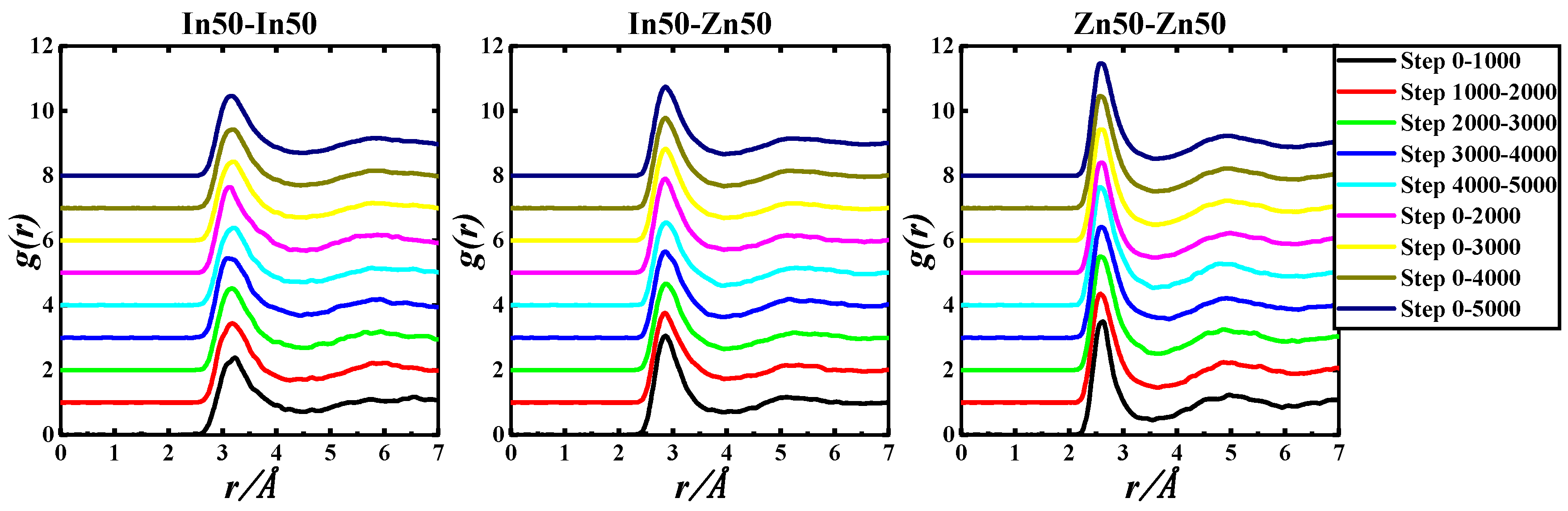
Metals 14 00102 g001
Figure 2. gIn-In(r), gIn-Zn(r), and gZn-Zn(r) of the Pb50Sn50-1050 K system based on 5000 step PRDF data.
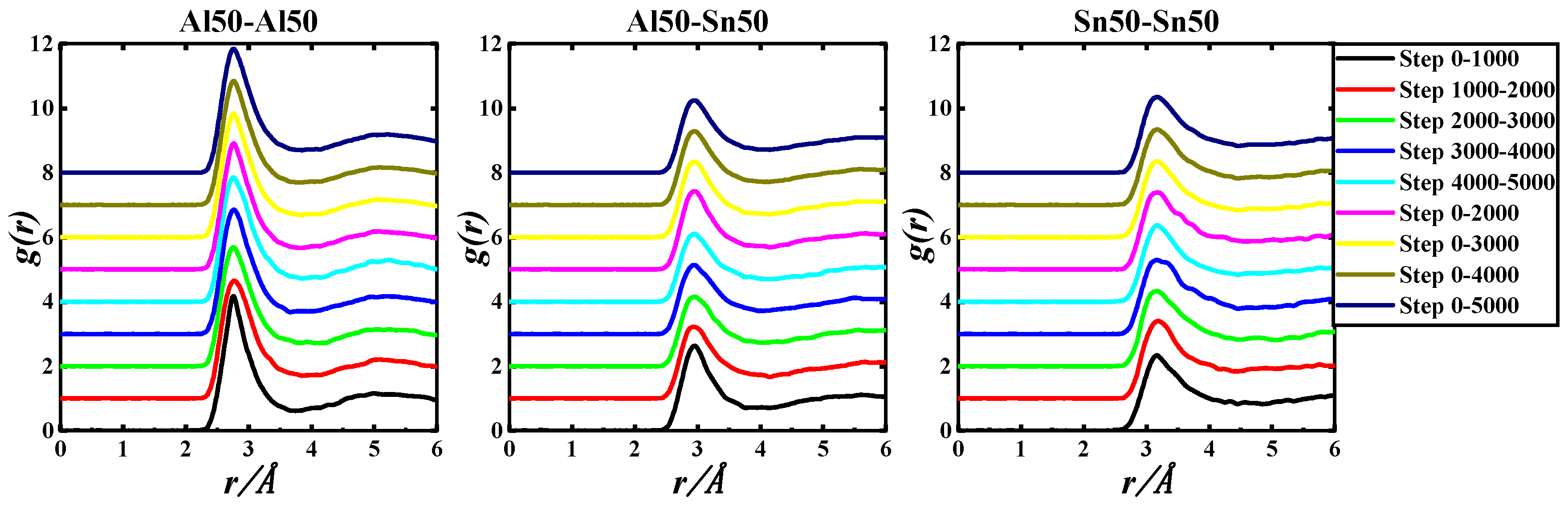
Metals 14 00102 g002
Figure 3. gAl-Al(r), gAl-Sn(r), and gSn-Sn(r) of the Al50Sn50-973 K system based on 5000 step PRDF data.
Metals 14 00102 g003
Figure 4. gIn-In(r), gIn-Zn(r), and gZn-Zn(r) of the In50Zn50-730 K system based on 5000 step PRDF data.
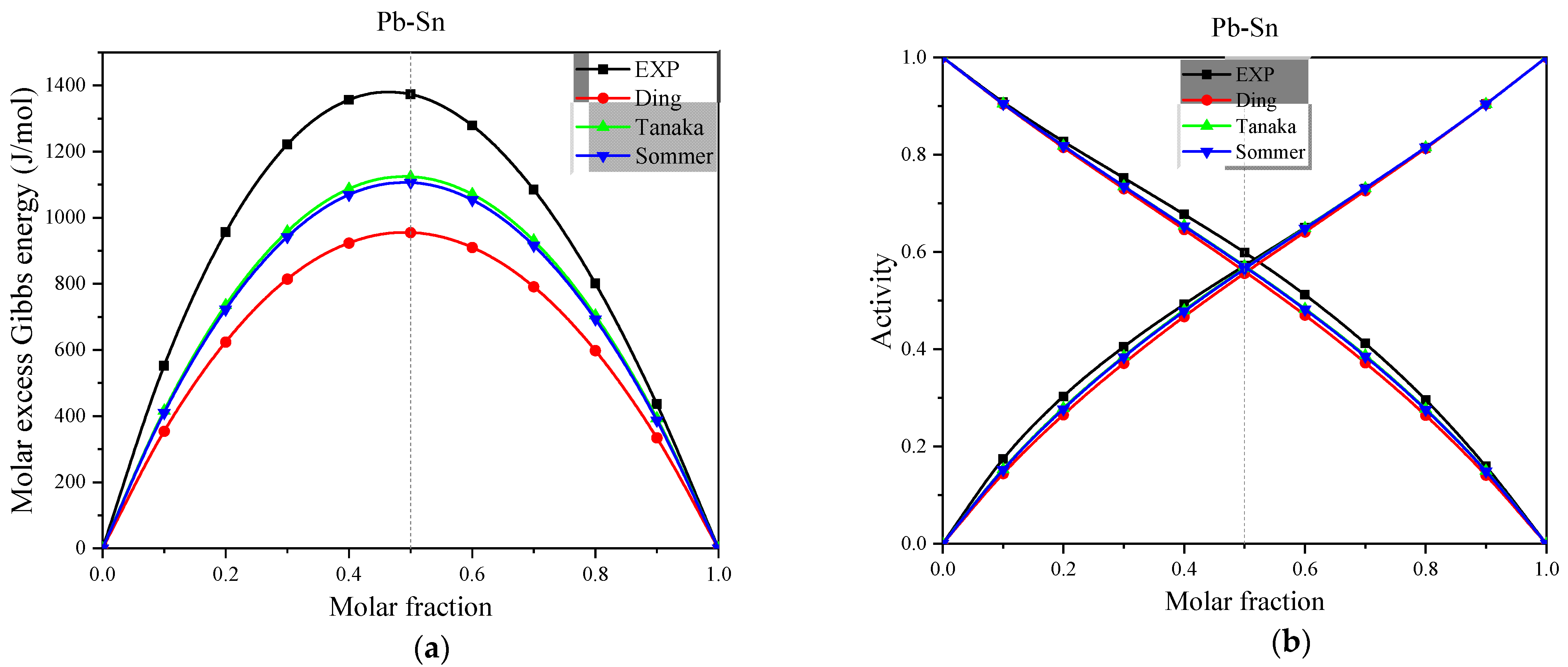
Metals 14 00102 g004
Figure 5. (a) The experimental and calculated values of molar excess Gibbs energy for the full concentration of Pb-Sn alloys in the Miedema model at 1050 K, (b) The experimental and calculated values of activity for the full concentration of Pb-Sn alloys in the Miedema model at 1050 K.
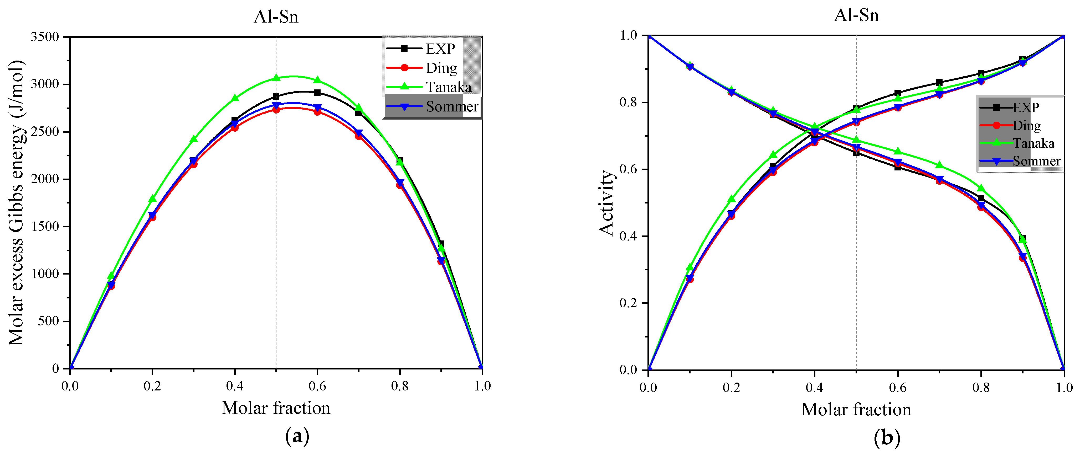
Metals 14 00102 g005
Figure 6. (a) The experimental and calculated values of molar excess Gibbs energy for the full concentration of Al-Sn alloys in the Miedema model at 973 K, (b) The experimental and calculated values of activity for the full concentration of Al-Sn alloys in the Miedema model at 973 K.
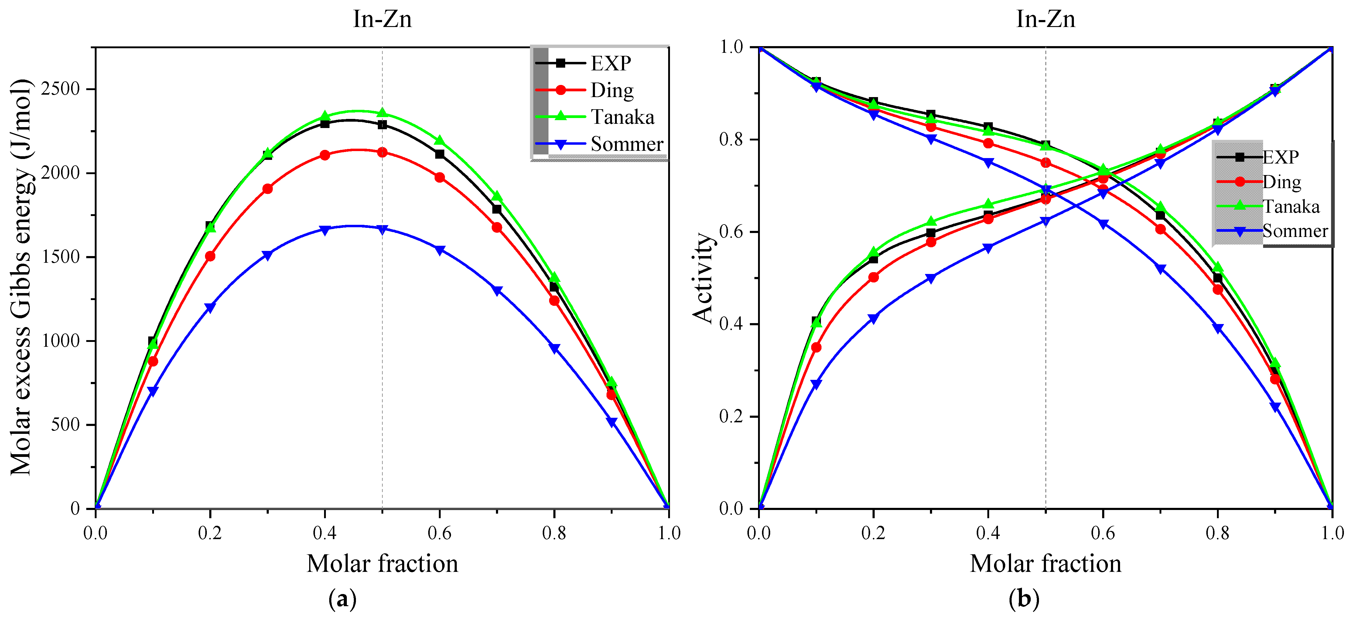
Metals 14 00102 g006
Figure 7. (a) The experimental and calculated values of molar excess Gibbs energy for the full concentration of In-Zn alloys in the Miedema model at 730 K, (b) The experimental and calculated values of activity for the full concentration of In-Zn alloys in the Miedema model at 730 K.
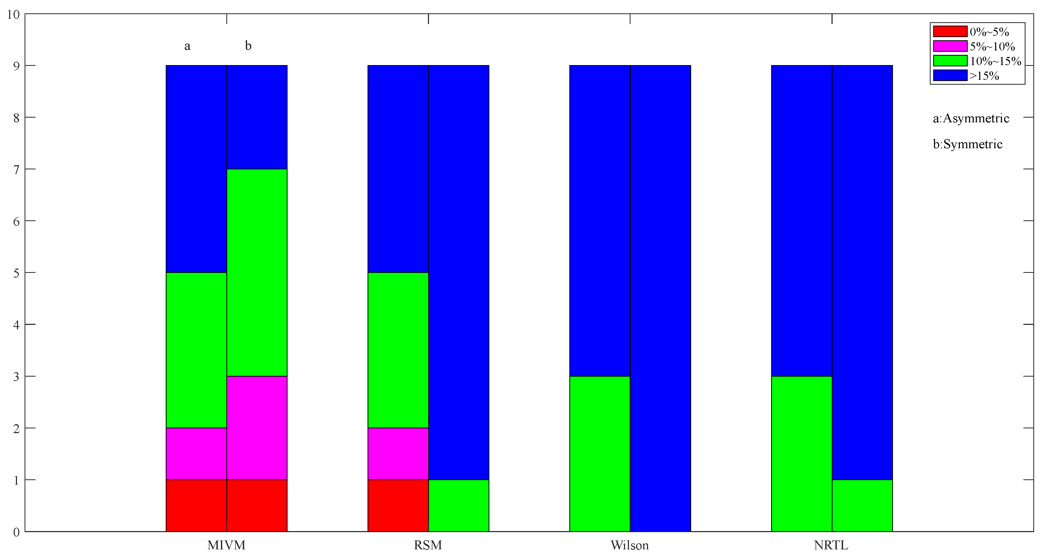
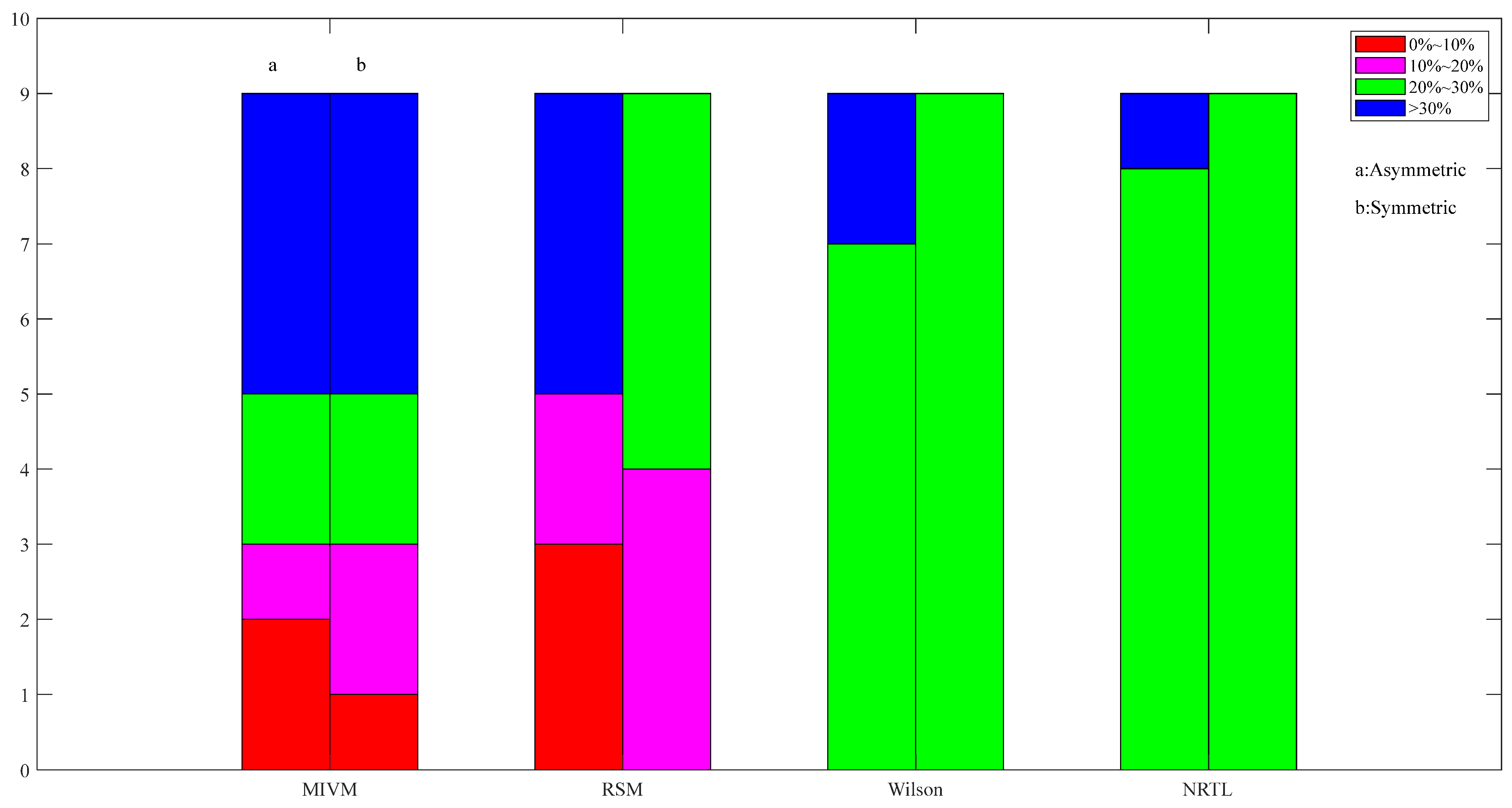
Metals 14 00102 g007
Figure 8. Images of asymmetric and symmetric method activity ARD calculations for Pb50-Sn50 alloys in four models at 1050 K.
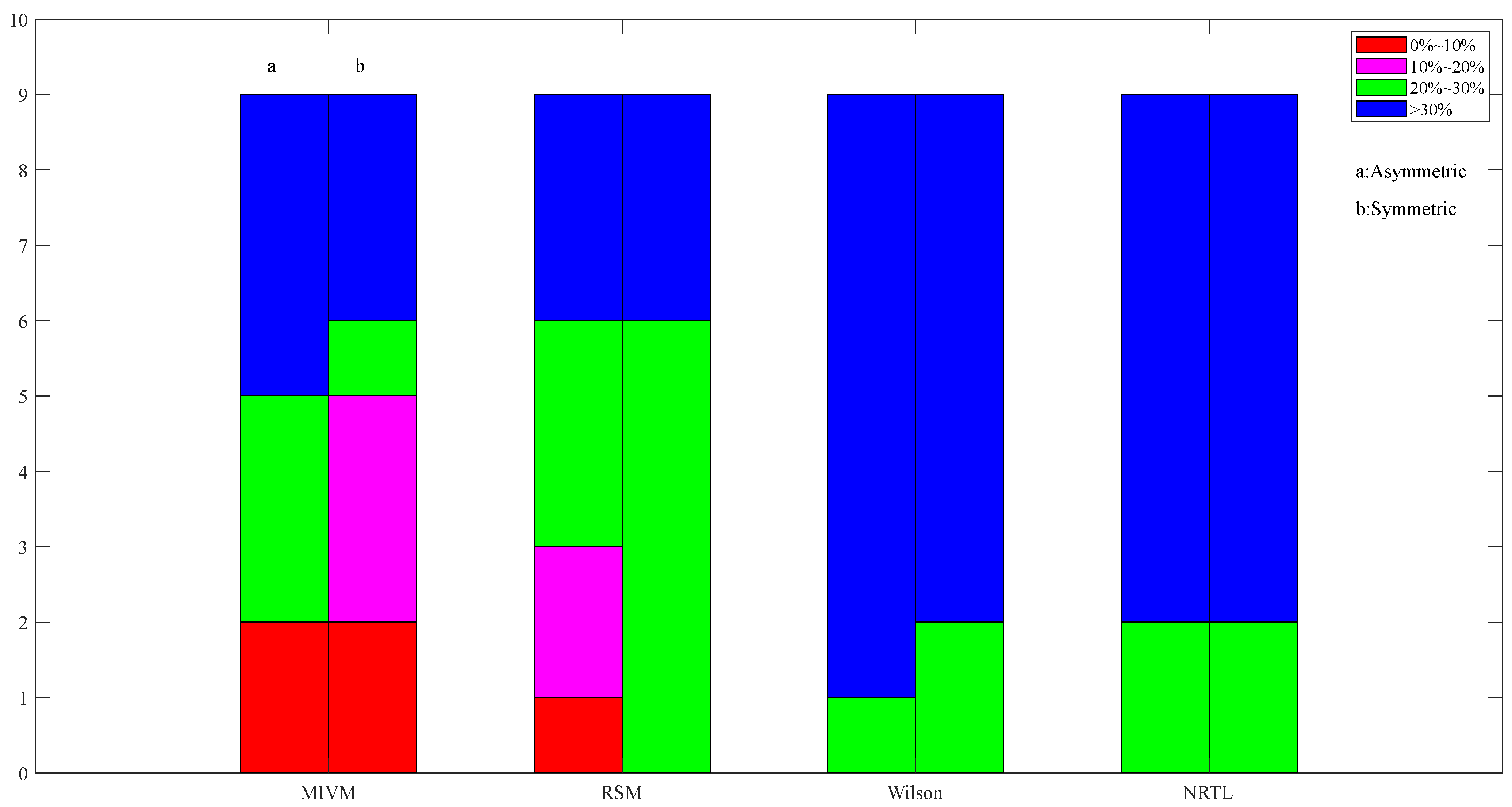
Metals 14 00102 g008
Figure 9. Images of asymmetric and symmetric method activity ARD calculations for Al50-Sn50 alloys in four models at 973 K.
Metals 14 00102 g009
Figure 10. Images of asymmetric and symmetric method activity ARD calculations for In50-Zn50 alloys in four models at 730 K.
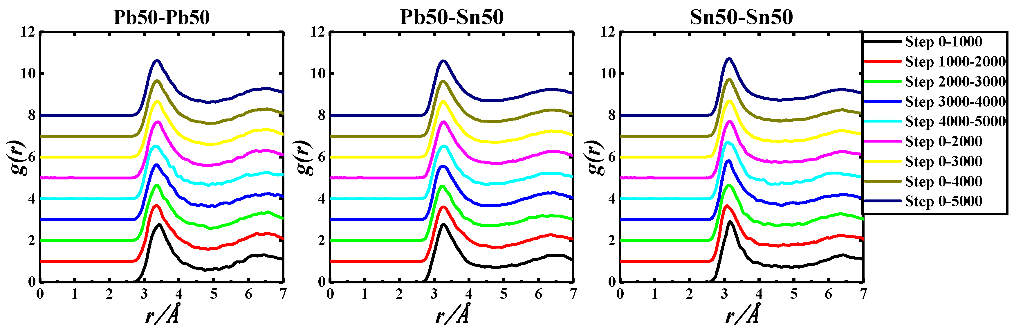
Metals 14 00102 g010
Table 1. The three key coordinate points of gPb-Pb(r), gPb-Sn(r), and gSn-Sn(r) in the Pb50Sn50-1050 K system.
ParametersStep of Pb50-Sn50 (1050 K)
0–10001000–20002000–30003000–40004000–50000–20000–30000–40000–5000
r0 i-i2.650 2.650 2.650 2.650 2.650 2.650 2.650 2.650 2.650
g(r0)i-i0.004 0.004 0.004 0.004 0.005 0.004 0.004 0.004 0.004
rm i-i3.450 3.350 3.350 3.350 3.350 3.350 3.350 3.350 3.350
g(rm)i-i2.751 2.671 2.634 2.628 2.521 2.645 2.641 2.638 2.615
r1 i-i4.750 4.850 4.850 4.550 4.850 4.750 4.850 4.850 4.850
g(r1)i-i0.577 0.581 0.594 0.680 0.646 0.590 0.595 0.604 0.613
r0 i-j2.550 2.650 2.550 2.650 2.550 2.550 2.550 2.550 2.550
g(r0)i-j0.002 0.011 0.001 0.007 0.001 0.001 0.001 0.001 0.001
rm i-j3.250 3.250 3.250 3.250 3.250 3.250 3.250 3.250 3.250
g(rm)i-j2.748 2.601 2.614 2.547 2.508 2.675 2.654 2.627 2.603
r1 i-j4.750 4.950 4.450 4.450 4.550 4.750 4.750 4.750 4.750
g(r1)i-j0.699 0.671 0.704 0.669 0.677 0.688 0.700 0.696 0.700
r0 j-j2.550 2.550 2.550 2.450 2.550 2.550 2.550 2.450 2.450
g(r0)j-j0.003 0.002 0.013 0.001 0.001 0.002 0.006 0.001 0.001
rm j-j3.150 3.050 3.150 3.150 3.050 3.150 3.150 3.150 3.150
g(rm)j-j2.874 2.632 2.647 2.807 2.667 2.712 2.690 2.719 2.706
r1 j-j4.150 4.150 4.150 4.650 4.350 4.350 4.150 4.550 4.550
g(r1)j-j0.790 0.801 0.756 0.673 0.697 0.748 0.783 0.729 0.724
Table 2. The three key coordinate points of gAl-Al(r), gAl-Sn(r), and gSn-Sn(r) in the Al50Sn50-973 K system.
ParametersStep of Al50-Sn50 (973 K)
0–10001000–20002000–30003000–40004000–50000–20000–30000–40000–5000
r0 i-i1.850 2.150 2.250 2.250 2.250 1.850 1.850 1.850 1.850
g(r0)i-i0.002 0.001 0.001 0.004 0.005 0.001 0.001 0.001 0.001
rm i-i2.750 2.750 2.750 2.750 2.750 2.750 2.750 2.750 2.750
g(rm)i-i4.165 3.629 3.686 3.843 3.850 3.897 3.827 3.831 3.834
r1 i-i3.750 3.850 3.850 3.650 3.850 3.850 3.850 3.850 3.850
g(r1)i-i0.612 0.708 0.722 0.676 0.717 0.669 0.687 0.691 0.697
r0 i-j1.750 2.350 2.350 2.250 2.350 1.750 1.750 1.750 1.750
g(r0)i-j0.001 0.002 0.001 0.001 0.002 0.001 0.001 0.001 0.001
rm i-j2.950 2.950 2.950 2.950 2.950 2.950 2.950 2.950 2.950
g(rm)i-j2.634 2.219 2.149 2.134 2.094 2.426 2.334 2.284 2.246
r1 i-j3.750 4.150 4.050 4.050 3.850 3.750 3.750 3.750 3.750
g(r1)i-j0.713 0.667 0.728 0.712 0.770 0.754 0.767 0.777 0.776
r0 j-j2.450 2.550 2.550 2.550 2.550 2.450 2.450 2.450 2.450
g(r0)j-j0.003 0.003 0.005 0.004 0.001 0.001 0.001 0.001 0.001
rm j-j3.150 3.150 3.150 3.150 3.150 3.150 3.150 3.150 3.150
g(rm)j-j2.324 2.383 2.319 2.286 2.381 2.354 2.342 2.328 2.339
r1 j-j4.450 4.450 4.450 4.450 4.550 4.450 4.450 4.450 4.450
g(r1)j-j0.824 0.838 0.829 0.783 0.866 0.831 0.830 0.818 0.833
Table 3. The three key coordinate points of gIn-In(r), gIn-Zn(r), and gZn-Zn(r) in the In50Zn50-730 K system.
ParametersStep of In50-Zn50 (730 K)
0–10001000–20002000–30003000–40004000–50000–20000–30000–40000–5000
r0 i-i2.250 2.550 2.450 2.550 2.550 2.250 2.250 2.250 2.250
g(r0)i-i0.003 0.010 0.001 0.011 0.005 0.002 0.001 0.001 0.001
rm i-i3.250 3.150 3.150 3.150 3.150 3.250 3.150 3.150 3.150
g(rm)i-i2.368 2.424 2.505 2.429 2.651 2.370 2.397 2.405 2.454
r1 i-i4.150 4.250 3.950 4.450 4.250 4.150 4.150 4.150 4.150
g(r1)i-i0.777 0.680 0.861 0.680 0.704 0.744 0.757 0.771 0.775
r0 i-j2.150 2.350 2.350 2.350 2.350 2.150 2.150 2.150 2.150
g(r0)i-j0.001 0.010 0.011 0.004 0.006 0.001 0.001 0.001 0.001
rm i-j2.850 2.850 2.850 2.850 2.850 2.850 2.850 2.850 2.850
g(rm)i-j3.045 2.760 2.640 2.654 2.536 2.903 2.815 2.775 2.727
r1 i-j3.950 3.950 3.950 3.950 3.950 3.950 3.950 3.950 3.950
g(r1)i-j0.695 0.725 0.648 0.630 0.603 0.710 0.689 0.675 0.660
r0 j-j2.050 2.050 2.150 2.150 2.150 2.050 2.050 2.050 2.050
g(r0)j-j0.001 0.001 0.012 0.009 0.011 0.001 0.001 0.001 0.001
rm j-j2.650 2.550 2.550 2.650 2.550 2.650 2.650 2.650 2.550
g(rm)j-j3.455 3.307 3.452 3.353 3.605 3.340 3.371 3.366 3.404
r1 j-j3.550 3.650 3.650 3.850 3.550 3.550 3.550 3.650 3.650
g(r1)j-j0.455 0.457 0.505 0.574 0.542 0.470 0.486 0.521 0.527
Table 4. Parameters for Miedema model calculation of Pb-Sn, Al-Sn, In-Zn systerms [42].
MetalΦnws1/3V2/3μαTm/KTb/Kr/p
Pb4.11.156.90.040.73105020222.1
Al4.21.394.60.070.7393327931.9
Sn4.151.246.40.040.7350528752.1
In3.91.176.30.070.7343023451.9
Zn4.11.324.40.10.7369311811.4
Table 5. Parameters of four models were calculated for Pb-Sn, Al-Sn, and In-Zn systems by asymmetric and symmetric methods.
SystemStepMIVMRSMWilsonNRTL
AsymSymAsymSymAsymSymAsymSym
BijBjiBijBjiw/kTw/kTAijAjiAijAjiτijτjiτijτji
Pb50-Sn50 (1050 K)0–10000.87 0.97 0.98 0.94 1.08 0.25 0.85 1.00 0.83 1.12 0.03 0.14 0.06 0.02
1000–20000.84 0.96 1.01 0.98 1.49 0.04 0.84 0.96 0.86 1.16 0.05 0.18 0.02 −0.01
2000–30000.94 1.09 0.96 1.02 0.14 0.06 0.95 1.08 0.90 1.09 −0.08 0.06 −0.02 0.04
3000–40001.09 0.98 0.92 1.02 0.37 0.15 0.86 1.24 0.90 1.05 0.02 −0.08 −0.02 0.09
4000–50000.94 1.05 1.01 0.98 0.09 0.05 0.92 1.08 0.86 1.15 −0.05 0.06 0.02 −0.01
0–20000.95 0.98 0.95 1.02 0.51 0.11 0.85 1.08 0.89 1.09 0.03 0.05 −0.02 0.05
0–30000.87 1.00 0.96 1.02 0.86 0.09 0.88 1.00 0.89 1.09 0.00 0.13 −0.02 0.05
0–40000.99 1.00 0.95 1.02 0.11 0.10 0.87 1.13 0.89 1.08 0.01 0.01 −0.02 0.06
0–50000.98 0.99 0.94 1.01 0.18 0.16 0.87 1.12 0.89 1.07 0.01 0.02 −0.01 0.07
Al50-Sn50 (973 K)0–10001.14 0.79 1.18 0.70 0.54 0.50 1.19 0.76 1.06 0.78 0.24 −0.13 0.36 −0.17
1000–20000.89 0.64 0.98 0.64 3.50 1.18 0.97 0.59 0.96 0.65 0.44 0.12 0.45 0.02
2000–30000.90 0.68 0.93 0.60 3.01 1.48 1.02 0.60 0.90 0.62 0.39 0.10 0.51 0.07
3000–40000.88 0.59 0.95 0.59 3.93 1.46 0.89 0.58 0.89 0.63 0.53 0.13 0.53 0.05
4000–50000.93 0.66 0.89 0.56 2.90 1.76 0.99 0.62 0.85 0.59 0.42 0.07 0.58 0.12
0–20001.08 0.79 1.08 0.67 0.89 0.83 1.18 0.72 1.01 0.72 0.24 −0.08 0.40 −0.08
0–30001.05 0.78 1.03 0.65 1.11 1.05 1.17 0.70 0.98 0.68 0.26 −0.05 0.43 −0.03
0–40001.03 0.76 1.01 0.63 1.32 1.15 1.15 0.69 0.95 0.67 0.27 −0.03 0.46 −0.01
0–50001.01 0.75 0.98 0.62 1.55 1.27 1.12 0.67 0.93 0.65 0.29 −0.01 0.48 0.02
In50-Zn50 (730 K)0–10000.95 1.08 0.81 1.22 0.17 0.24 0.66 1.56 0.74 1.33 −0.08 0.05 −0.20 0.21
1000–20000.93 1.05 0.86 1.14 0.16 0.00 0.64 1.53 0.69 1.41 −0.05 0.07 −0.13 0.15
2000–30000.85 0.89 0.79 1.04 1.61 0.42 0.54 1.39 0.64 1.29 0.12 0.16 −0.04 0.24
3000–40000.93 1.06 0.73 1.04 0.09 0.94 0.65 1.52 0.63 1.20 −0.06 0.08 −0.04 0.32
4000–50000.76 0.96 0.74 0.96 1.88 0.78 0.58 1.25 0.58 1.22 0.05 0.27 0.04 0.30
0–20000.92 1.04 0.79 1.13 0.24 0.58 0.64 1.51 0.69 1.30 −0.04 0.09 −0.13 0.23
0–30000.88 1.01 0.76 1.17 0.66 0.47 0.62 1.44 0.71 1.25 −0.01 0.13 −0.16 0.28
0–40000.91 1.00 0.75 1.14 0.58 0.59 0.61 1.49 0.69 1.23 0.00 0.10 −0.13 0.29
0–50000.88 0.98 0.83 1.10 0.82 0.16 0.60 1.45 0.67 1.36 0.02 0.12 −0.09 0.18
Table 6. Comparison of experimental and calculated values of molar excess Gibbs energy and activity for Pb-Sn alloys all at full concentration in the Miedema model at 1050 K.
Molar Excess Gibbs Energy (J/mol)
xiExpDingTanakaSommer
0.9436334393387
0.8801598704693
0.71085791931916
0.6127991010711054
0.5137395511241106
0.4135692310871069
0.31221814958942
0.2956624735723
0.1552354416410
ARD%30.11%17.73%19.05%
SD325197210
Activity
xiai-Expaj-Expai-Dingaj-Dingai-Tanakaaj-Tanakaai-Sommeraj-Sommer
0.90.9040.1590.9040.1410.9040.1500.9040.149
0.80.8140.2960.8130.2640.8150.2770.8150.276
0.70.7300.4120.7260.3720.7310.3870.7310.385
0.60.6500.5120.6410.4700.6490.4830.6480.482
0.50.5720.5990.5560.5600.5660.5710.5650.570
0.40.4920.6770.4670.6460.4800.6540.4780.653
0.30.4050.7520.3710.7300.3850.7350.3840.735
0.20.3030.8270.2650.8150.2790.8180.2770.818
0.10.1740.9080.1440.9040.1530.9050.1520.905
ARD% of Single Component5.37%6.18%3.22%3.89%3.43%4.13%
SD of Single Component0.0220.0290.0130.020.0140.021
ARD%5.77%3.55%3.78%
SD0.0260.0170.018
Table 7. Comparison of experimental and calculated values of molar excess Gibbs energy and activity for Al-Sn alloys all at full concentration in the Miedema model at 973 K.
Molar Excess Gibbs Energy (J/mol)
xiExpDingTanakaSommer
0.91318113012661149
0.82194193721711970
0.72703245427502498
0.62911271130392761
0.52870273330632784
0.42624254228492591
0.32200215824182200
0.21619159617881628
0.1887872977890
ARD%6.11%6.34%4.55%
SD160147130
Activity
xiai-Expaj-Expai-Dingaj-Dingai-Tanakaaj-Tanakaai-Sommeraj-Sommer
0.90.9270.3930.9190.3350.9210.3880.9190.343
0.80.8870.5140.8640.4870.8720.5420.8650.495
0.70.8590.5670.8230.5660.8390.6110.8250.573
0.60.8280.6060.7840.6180.8100.6520.7880.624
0.50.7820.6500.7400.6640.7760.6870.7450.668
0.40.7110.7020.6800.7110.7250.7260.6860.714
0.30.6090.7620.5910.7660.6420.7740.5990.768
0.20.4680.8310.4610.8310.5100.8350.4680.832
0.10.2740.9090.2710.9080.3060.9090.2770.908
ARD% of Single Component3.12%2.93%3.94%3.68%2.58%2.89%
SD of Single Component0.0280.0220.0240.0280.0250.021
ARD%3.03%3.81%2.74%
SD0.0250.0260.023
Table 8. Comparison of experimental and calculated values of molar excess Gibbs energy and activity for In-Zn alloys all at full concentration in the Miedema model at 730 K.
Molar Excess Gibbs Energy (J/mol)
xiExpDingTanakaSommer
0.9726679752523
0.8132112411375961
0.71785167718591305
0.62112197521901546
0.52288212423541670
0.42295210723351666
0.32105190721141516
0.21686150616691203
0.11000879974706
ARD%8.08%2.68%27.71%
SD14450491
Activity
xiai-Expaj-Expai-Dingaj-Dingai-Tanakaaj-Tanakaai-Sommeraj-Sommer
0.90.910 0.300 0.908 0.281 0.909 0.315 0.906 0.223
0.80.835 0.500 0.832 0.475 0.836 0.522 0.823 0.393
0.70.772 0.636 0.769 0.606 0.777 0.653 0.750 0.522
0.60.719 0.728 0.716 0.692 0.730 0.735 0.685 0.619
0.50.674 0.788 0.671 0.750 0.692 0.784 0.625 0.693
0.40.636 0.827 0.628 0.792 0.659 0.816 0.567 0.752
0.30.598 0.854 0.578 0.828 0.621 0.843 0.501 0.803
0.20.542 0.882 0.502 0.867 0.555 0.874 0.414 0.855
0.10.407 0.925 0.350 0.920 0.401 0.922 0.272 0.916
ARD% of Single Component3.07%3.93%1.81%1.91%11.16%12.34%
SD of Single Component0.0240.0270.0140.0120.0770.082
ARD%3.50%1.86%11.75%
SD0.0260.0130.079
Table 9. The SD and ARD of molar excess Gibbs energy and activity of Pb50Sn50 alloys were estimated by asymmetric method at 1050 K.
GEm and aStep MIVMRSMWilsonNRTL
ARD%SDARD%SDARD%SDARD%SD
GEm (J/mol)0~100061.4%64272.4%76074.2%78773.7%782
1000~2000107.9%1131137.0%144166.2%70465.9%701
2000~3000131.5%1390121.8%1288104.0%1100103.3%1093
3000~4000166.8%1758159.8%1685112.5%1190109.8%1161
4000~500091.2%96586.0%91198.3%104097.7%1034
0~200025.4%26537.0%38879.4%93987.6%928
0~300022.7%25018.1%19988.7%84279.2%839
0~400085.1%90282.6%87698.8%104597.4%1031
0~500074.7%79371.6%76097.1%102795.8%1014
Average85.2%89987.4%92391.0%96490.0%954
a0~100013.4%0.05716.2%0.06913.1%0.05813.0%0.057
1000~200025.8%0.10834.8%0.14411.9%0.05211.8%0.052
2000~300021.2%0.09420.0%0.08817.5%0.07717.5%0.077
3000~400025.6%0.11424.7%0.1118.7%0.08318.4%0.081
4000~500015.7%0.06914.9%0.06616.7%0.07416.7%0.074
0~20005.2%0.0227.8%0.03415.3%0.06815.1%0.067
0~30004.5%0.0213.7%0.01713.9%0.06113.9%0.061
0~400014.8%0.06514.4%0.06416.8%0.07416.6%0.073
0~500013.2%0.05812.7%0.05616.5%0.07316.4%0.072
Average15.5%0.06816.6%0.07215.6%0.06915.5%0.068
Table 10. The SD and ARD of molar excess Gibbs energy and activity of Pb50Sn50 alloys were estimated by symmetric method at 1050 K.
GEm and aStep MIVMRSMWilsonNRTL
ARD%SDARD%SDARD%SDARD%SD
GEm (J/mol)0~100014.2%17159.7%63288.7%93985.9%911
1000~2000117.3%1239106.0%1122104.6%1106102.4%1083
2000~300083.3%88390.8%96297.5%103296.8%1024
3000~400053.1%56576.7%81392.1%97691.7%971
4000~5000123.7%1306108.5%1148105.7%1118103.3%1092
0~200062.3%66282.5%87494.3%99893.5%990
0~300071.7%76186.2%91495.8%101495.0%1006
0~400066.8%71083.9%88994.9%100494.2%997
0~500045.3%48374.3%78891.5%96990.8%962
Average70.8%75385.4%90596.1%101794.8%1004
a0~10003.2%0.01613.7%0.0615.3%0.06815.0%0.066
1000~200019.4%0.08617.4%0.07717.6%0.07817.3%0.076
2000~300014.5%0.06416.3%0.07216.6%0.07316.5%0.073
3000~40009.7%0.04315.2%0.06715.8%0.0715.8%0.07
4000~500020.2%0.0917.5%0.07717.8%0.07917.4%0.077
0~200011.2%0.04915.7%0.06916.1%0.07116.0%0.071
0~300012.7%0.05616.0%0.0716.3%0.07216.3%0.072
0~400012.0%0.05315.8%0.0716.2%0.07216.1%0.071
0~50008.4%0.03715.0%0.06615.7%0.06915.6%0.069
Average12.4%0.05515.8%0.0716.4%0.07216.2%0.072
Table 11. The SD and ARD of molar excess Gibbs energy and activity of Al50Sn50 alloys were estimated by asymmetric method at 973 K.
GEm and aStep MIVMRSMWilsonNRTL
ARD%SDARD%SDARD%SDARD%SD
GEm (J/mol)0~100060.4%135943.6%98694.9%213992.0%2075
1000~200071.1%1600100.0%224265.5%148160.0%1361
2000~300056.5%127076.4%171569.8%157764.7%1467
3000~400089.5%2017120.7%271659.1%133852.6%1197
4000~500051.1%115470.5%158769.7%157464.6%1464
0~200055.6%124938.5%88191.3%205788.0%1985
0~300038.1%85823.3%55088.8%200185.3%1925
0~400022.4%5069.1%25386.3%194682.6%1866
0~50006.0%14810.5%22783.6%188579.7%1801
Average50.1%112954.7%124078.8%177874.4%1682
a0~100020.2%0.13215.7%0.10430.9%0.20230.7%0.201
1000~200050.8%0.3388.8%0.56523.2%0.15622.6%0.15
2000~300036.6%0.23657.4%0.36524.5%0.16423.8%0.157
3000~400072.9%0.483126.6%0.80921.4%0.14520.9%0.139
4000~500032.1%0.20951.1%0.32524.4%0.16324.0%0.158
0~200020.4%0.13414.8%0.10430.0%0.19729.7%0.194
0~300014.8%0.0989.9%0.07429.4%0.19329.0%0.19
0~40009.1%0.0616.6%0.05128.8%0.1928.4%0.186
0~50002.8%0.0228.3%0.05428.1%0.18627.7%0.182
Average28.8%0.25658.3%0.37626.7%0.17726.3%0.173
Table 12. The SD and ARD of molar excess Gibbs energy and activity of Al50Sn50 alloys were estimated by symmetric method at 973 K.
GEm and aStep MIVMRSMWilsonNRTL
ARD%SDARD%SDARD%SDARD%SD
GEm (J/mol)0~100045.1%100865.2%148487.9%198284.5%1906
1000~200037.9%86217.8%46671.1%160666.0%1495
2000~300067.9%153612.3%23663.6%143957.6%1308
3000~400063.0%142812.2%23363.7%144357.6%1307
4000~5000106.1%209523.4%54656.9%129049.9%1136
0~20004.4%8741.8%97079.5%179575.4%1703
0~300029.8%68527.1%65574.3%167869.6%1574
0~400044.9%102619.9%50871.7%162066.6%1508
0~500063.1%143512.9%34968.7%155363.3%1434
Average51.4%112925.8%60570.8%160165.6%1486
a0~100016.2%0.10427.8%0.18329.2%0.19229.4%0.192
1000~200022.0%0.14520.4%0.13724.8%0.16524.6%0.162
2000~300047.7%0.31516.1%0.11222.7%0.15322.4%0.148
3000~400042.9%0.28516.5%0.11422.8%0.15322.6%0.149
4000~500077.8%0.52112.1%0.08920.7%0.14120.3%0.135
0~20001.6%0.0124.4%0.16227.1%0.17927.1%0.178
0~300015.8%0.10522.0%0.14725.7%0.17125.6%0.169
0~400025.2%0.16720.7%0.13925.0%0.16624.9%0.164
0~500038.1%0.25219.2%0.1324.2%0.16124.0%0.158
Average31.9%0.21219.9%0.13524.7%0.16524.6%0.162
Table 13. The SD and ARD of molar excess Gibbs energy and activity of In50Zn50 alloys were estimated by asymmetric method at 730 K.
GEm and aStep MIVMRSMWilsonNRTL
ARD%SDARD%SDARD%SDARD%SD
GEm (J/mol)0~1000123.0%2197111.2%1986108.0%1929101.8%1818
1000~200098.4%175789.5%1598104.4%186598.2%1753
2000~30008.4%1408.4%14389.2%159181.8%1463
3000~4000103.8%185593.8%1675105.0%187498.9%1767
4000~500012.5%23022.9%42084.7%151180.1%1432
0~200092.2%164784.0%1500103.3%184497.2%1736
0~300063.2%113157.1%101998.5%175892.7%1655
0~400067.9%121562.0%1108100.0%178593.6%1671
0~500051.3%92146.1%82697.2%173590.9%1625
Average69.0%123363.9%114298.9%176692.8%1658
a0~100038.2%0.25934.6%0.23435.2%0.23833.9%0.229
1000~200033.0%0.22432.2%0.21834.4%0.23333.0%0.223
2000~30005.3%0.0366.9%0.04630.8%0.2128.9%0.196
3000~400034.2%0.23231.9%0.21634.5%0.23333.2%0.225
4000~50006.8%0.04713.9%0.09629.6%0.20228.4%0.193
0~200031.6%0.21429.5%0.234.1%0.23132.8%0.222
0~300023.8%0.16221.8%0.1533.0%0.22431.7%0.215
0~400025.2%0.17123.4%0.1633.4%0.22631.9%0.216
0~500020.1%0.13818.3%0.12832.7%0.22231.2%0.212
Average24.2%0.16523.6%0.16133.1%0.22431.7%0.215
Table 14. The SD and ARD of molar excess Gibbs energy and activity of In50Zn50 alloys were estimated by symmetric method at 730 K.
GEm and aStep MIVMRSMWilsonNRTL
ARD%SDARD%SDARD%SDARD%SD
GEm (J/mol)0~100090.9%162184.0%150098.0%175094.6%1690
1000~2000113.6%2029100.0%1785104.7%186999.7%1781
2000~300043.9%78472.6%129494.0%167889.2%1594
3000~40009.6%17838.3%69282.5%147279.4%1419
4000~500010.2%19248.9%86885.6%152880.6%1442
0~200046.4%82462.3%111191.8%163988.4%1579
0~300060.2%107069.2%124091.8%164089.1%1592
0~400042.0%74461.4%110289.4%159786.7%1549
0~500085.9%153589.4%1595100.7%179895.7%1710
Average55.9%99769.6%124393.2%166389.3%1595
a0~100031.3%0.21231.2%0.21132.9%0.22332.4%0.219
1000~200036.3%0.24633.4%0.22634.5%0.23333.4%0.226
2000~300017.6%0.1229.9%0.20332.0%0.21730.9%0.209
3000~40005.1%0.03624.1%0.16529.1%0.19828.3%0.192
4000~50005.7%0.0426.2%0.17929.9%0.20428.6%0.194
0~200018.5%0.12527.9%0.18931.4%0.21430.8%0.208
0~300022.9%0.15429.3%0.19931.4%0.21331.1%0.211
0~400017.0%0.11428.1%0.19130.8%0.2130.4%0.206
0~500030.0%0.20332.1%0.21833.6%0.22732.5%0.22
Average20.5%0.13929.1%0.19831.7%0.21530.9%0.21
Disclaimer/Publisher’s Note: The statements, opinions and data contained in all publications are solely those of the individual author(s) and contributor(s) and not of MDPI and/or the editor(s). MDPI and/or the editor(s) disclaim responsibility for any injury to people or property resulting from any ideas, methods, instructions or products referred to in the content.

