Article

Automatic Control of Hot Metal Temperature

by
Yoshinari Hashimoto
1,*,
Ryosuke Masuda
1,
Max Mulder
2 and
Marinus M. (René) van Paassen
2
1
Cyber-Physical System Research and Development Department, JFE Steel Corp, Tokyo 100-0011, Japan
2
Faculty of Aerospace Engineering, Delft University of Technology, 2629 Delft, The Netherlands
*
Author to whom correspondence should be addressed.
Metals 2022, 12(10), 1624; https://doi.org/10.3390/met12101624
Submission received: 14 August 2022 / Revised: 17 September 2022 / Accepted: 22 September 2022 / Published: 28 September 2022
(This article belongs to the Special Issue Mathematical Modelling of the Ironmaking Blast Furnace)

Abstract

:
To achieve the automation of blast furnace operation, an automatic control system for hot metal temperature (HMT) was developed. Nonlinear model predictive control (NMPC) which predicts up to ten-hour-ahead HMT and calculates appropriate control actions of pulverized coal rate (PCR) was constructed. Simulation validation showed that the NMPC algorithm generates control actions similar to those by the operators and that HMT can be maintained within ±10 °C of the set point. The automatic control system using NMPC was then implemented in an actual plant. As a result, the developed control system suppressed the effects of disturbances, such as the changes in the coke ratio and blast volume, and successfully reduced the average control error of HMT by 4.6 °C compared to the conventional manual operation. The developed control system has contributed to the reduction of reducing agent rate (RAR) and CO2 emissions.

1. Introduction

In recent years, reduction of the reducing agent rate (RAR) of blast furnaces has been required in the steel industry, and it is difficult to maintain a stable furnace state under a low RAR condition by conventional manual operation. At the same time, cost reduction through equipment integration has also been demanded, requiring a high blast furnace production rate, which increases the risk of operational problems such as gas channeling due to excessive pressure drop of the furnace. While the blast furnace operation becomes difficult, the working population is expected to decrease in the future. Hence, process automation is considered necessary to maintain efficient and stable blast furnace operation [1,2].
Figure 1 shows an overview of the blast furnace process. Sintered iron ore and coke are charged from the furnace top, and hot blast is blown into the furnace from about 40 tuyeres arranged in the circumferential direction around the furnace. Auxiliary fuels such as pulverized coal (PC) and natural gas are also injected through the tuyeres. The sintered iron ore is reduced by CO and H2 gas while descending through the furnace and is eventually melted, and the hot metal and its viscous byproduct, slag, are tapped from the furnace bottom.
In the blast furnace process, it is crucial to maintain a constant hot metal temperature (HMT). When the HMT becomes too low, the slag drainage becomes difficult and it impairs furnace productivity. Conversely, an excessively high HMT also leads to excess consumption of the reducing agents. Reducing the variation in HMT makes it possible to keep the HMT near the lower bound, thereby reducing RAR.
A number of control methods have been developed to stabilize the HMT and Si content of hot metal, which are indicators of thermal status. Azadi et al. developed a prediction method for the Si content by combining first principles and a statistical model [3]. Jiang et al. developed an operation guidance system to maintain a constant Si content using a recurrent neural network based on feature selection [4]. Agrawal et al. developed a proactive thermal indicator based on the energy balance for controlling HMT [5]. Martín et al. applied fuzzy logic tools to predict future HMT [6]. Jiao et al. proposed a prediction method of HMT using collaborative multiple rank regression with the image data through tuyeres [7]. Hashimoto et al. developed an operation guidance system for HMT control based on a transient model and applied it to actual blast furnaces [8,9]. The operation guidance system predicts eight-hour-ahead HMT by the transient model and moving horizon estimation [10]. An operator behavior model that imitates the control actions of skilled operators for controlling HMT was also developed [11]. However, automatic HMT control that can be continuously used under adverse operating conditions, such as when the production rate is changed rapidly or the pressure drop fluctuates, has not been reported. To achieve more efficient and stable operation through process automation, this study is aiming at developing an automatic HMT control system that can be applied even under such hostile operating conditions.
Since the blast furnace process has an extremely large heat capacity, the time constant until the effect of control actions appears is also large. In addition, it takes several hours for the raw materials charged at the furnace top to descend through the furnace. Therefore, it is necessary to calculate appropriate control actions based on future predictions in order to control HMT accurately. In this study, a nonlinear model predictive control (NMPC) algorithm based on a two-dimensional (2D) transient model was newly developed and verified through simulations. An automatic control system using the NMPC algorithm was then implemented in a real plant and validated in the actual operation.
This paper is organized as follows. Section 2 describes the development of the NMPC algorithm. Section 3 presents the simulation verification and real operation result at the actual furnace. Section 4 concludes the paper.

2. Methodology

This section describes the development of the HMT control algorithm based on the 2D transient model of the blast furnace. First, the conventional manual operation by human operators and the disturbances that affect HMT control are discussed. A control algorithm that is compatible with the manual operation and can be clearly understood by the operators is then developed using NMPC. The input variables for the simulation using the 2D transient model, the manipulated variables, and the controlled variables are summarized in Table 1.

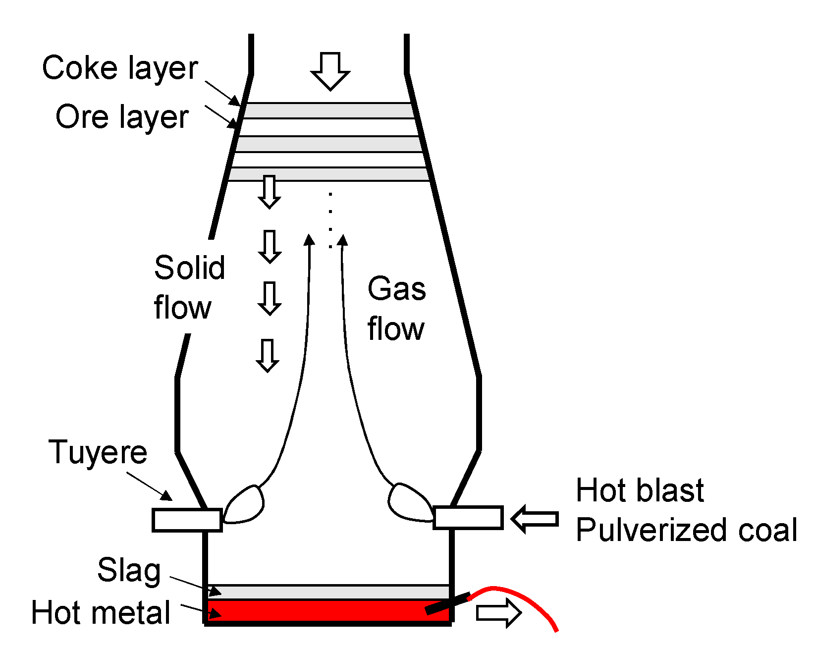
2.1. Conventional Manual Operation

Figure 2 shows the real operation data of the conventional manual operation for 120 h. The left column shows the variables which can be manipulated by the operators, and the right column shows the outcomes of the operation: HMT, the production rate (Prod), and the pressure drop from the tuyere level to the furnace top (ΔP). The red dashed lines and blue solid lines show the target values (or upper bound) and actual values, respectively. The vertical axes in the left column are all mean-centered, whereas those in the right column show the difference from the target value (or upper bound) at time zero. To decrease RAR, blast moisture (BM) and blast temperature (BT) are maintained at the lower bound and upper bound, respectively, and are not shown in the figure.
As shown in Figure 2a, the operators decreased the coke rate (CR) from 0 to 60 h to reduce operating costs. To compensate for the effect of the decreased CR on HMT, the target pulverized coal rate (PCR), i.e., the amount of pulverized coal per ton of hot metal, was increased during the same period, which is shown by the red dashed line in Figure 2b. The actual PCR shown by the blue solid line in Figure 2b is defined by
P C R = P C I / P r o d
where P C I (kg/min) is the PC flow rate and P r o d (t/min) is the production rate. Since the actual PCR fluctuates unintentionally depending on Prod, the PC flow rate in Figure 2c was manipulated so that the actual PCR matched the target PCR.
The operators also adjusted the blast volume (BV) and the enrichment oxygen flow rate (EO) shown in Figure 2d,e so that the actual Prod matched the target Prod in Figure 2g. Since ΔP in Figure 2h became high at 65 h, the gas flow was stabilized by decreasing BV and increasing CR at the same time, sacrificing Prod and the operating costs. Since ΔP decreased as a result of these control actions, BV was increased again at around 68 h to achieve the target Prod, and CR was gradually reduced from 70 h to 110 h.
In this manner, in the blast furnace operation, HMT is controlled by manipulating PCR and the PC flow rate, while the production rate is kept near its target by manipulating BV and EO. It is also necessary to avoid instability in the descent of burden materials due to the excessively high ΔP by decreasing BV and increasing CR. Therefore, the HMT controller that manipulates the PCR and PC flow rate must suppress the effects of disturbances due to the changes in CR, BV, and EO.
Here, the production rate was determined by the oxygen balance.
P r o d = V out O V in O O ore
where V in O is the amount of oxygen blown into the furnace, defined by V in O = B V × X O 2 + E O / 22.4 with the oxygen volume ratio X O 2 in BV. O ore is the oxygen amount in the unreduced iron ore which has to be reduced to produce a unit volume of hot metal. V out O is the oxygen amount in the top gas discharged from the furnace.
V out O = V top X CO + 2 X CO 2 + X H 2 O
where V top is the top gas flow rate and X ϕ is the volume ratio of gas component ϕ .

2.2. Transient Model

Various blast furnace models have been developed [12], including one-dimensional (1D) transient model [9,13], 2D steady-state model [14], 2D transient model [8,15,16], and three-dimensional (3D) transient model [17]. This study employs the two-dimensional (2D) transient model developed in the previous study [8]. The 2D transient model consists of four sub-models: a gas flow model, a material balance model, an energy balance model, and a solid flow model, considering 11 reactions listed in Table 2.
First, the gas flow model calculates the mass velocity of gas u g using Ergun’s equation.
P g = k g u g
· u g = R g
where k g is the gas flow resistance and R g is the gas generation rate.
The material balance model calculates the gas composition X 1 X 5 , oxidation degree of Fe X 6 , and iron composition X 7 X 9 .
· X i u g 0 = j m i , j R j
ρ fe X i t + · X i u fe = j m i , j R j
where u g 0 and u fe are the molar velocities of gas and liquid iron, respectively; m i , j is the molar ratio of substance i in the reaction j. For example, m 2 , 1 = 1 , m 3 , 1 = + 1 , and m 6 , 1 = 1 in the case of reaction 1 ( FeO x + CO = FeO x 1 + CO 2 ). The reaction rate R is the function of temperature and gas composition.
The energy balance model considers the reaction heat and the heat exchange among the gas, coke, and iron.
· C p , g T g u g = j η g , j Δ H R j R j + E g , fe T fe T g + E g , c T c T g + q
ρ c X c C p , c T c t = j η c , j Δ H R j R j + E fe , c T fe T c + E g , c T g T c
ρ fe X o C p , fe T fe t + · C p , fe T fe u fe = j η fe , j Δ H R j R j + E g , fe T g T fe + E fe , c T c T fe
The subscripts g, c, and fe denote gas, coke, and iron, respectively, and the subscript j means the index of the reactions listed in Table 2.
Finally, the solid flow model and the calculation procedure which can be found in the previous work [8] are briefly explained. The solid flow is expressed by the movement of calculation cells, which are updated at each time step. Equations (4)–(10) were discretized by the finite volume method in advance. The time step of the calculation was set to 5 min considering that it takes about 15 min to consume one set of iron layer and coke layer. Equations (4)–(6) and (8) which involve the gas flow were regarded steady-state since the residence time of the gas in the furnace is much shorter than the time step. At each time step, the gas flow, the material balance, and the energy balance are calculated using the implicit method while the solid flow is suspended. After the convergence, the heights of calculation cells are decreased according to the consumption rate of coke and iron ore, and the new calculation cells are generated at the furnace top so that the material surface level is maintained.
Figure 3 shows the simulation result by the 2D transient model using the real operation data for 60 h, where vertical axes are all mean-centered. HMT is shown in Figure 3g, where the blue solid line shows the actual value and the magenta dashed line shows the calculated value by the 2D transient model. In the actual blast furnace, HMT was measured by thermocouples after the hot metal was tapped from the furnace, and the measurement interval was about 30 min. The calculated HMT is the temperature of the iron at the height of the tuyere.
Since CR was lowered at 3 h and 7 h, the HMT decreased by about 40 °C from 5 to 28 h. The PCR increased around 24 h because the PC flow rate was almost constant while Prod decreased due to the decrease of EO. This increase in the PCR and the increase in CR at 20 h resulted in the increase of HMT by 30 °C from 30 h to 40 h. These transitions of HMT in the real plant were reproduced accurately by the 2D transient model, and accurate control of HMT is expected to be possible.

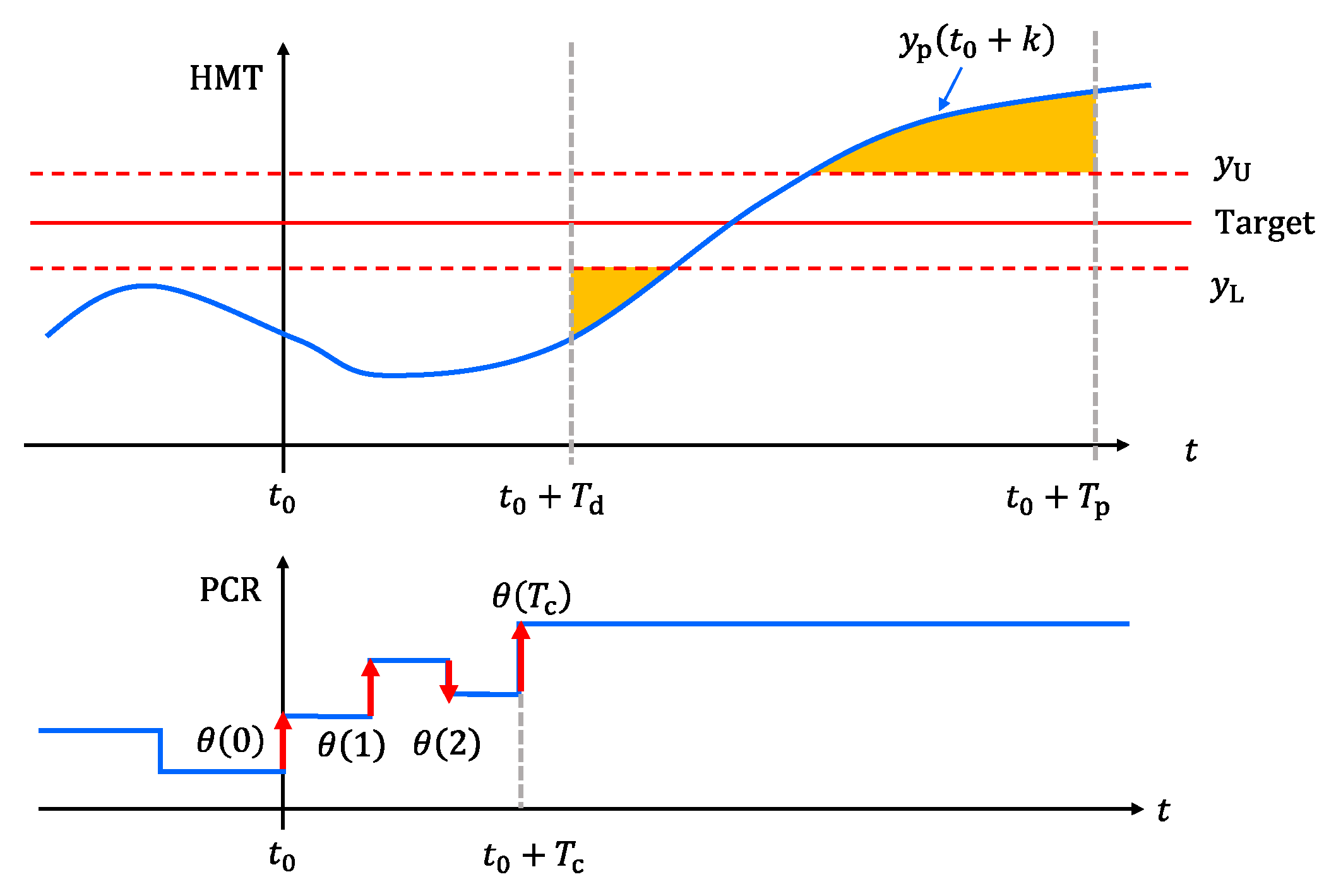
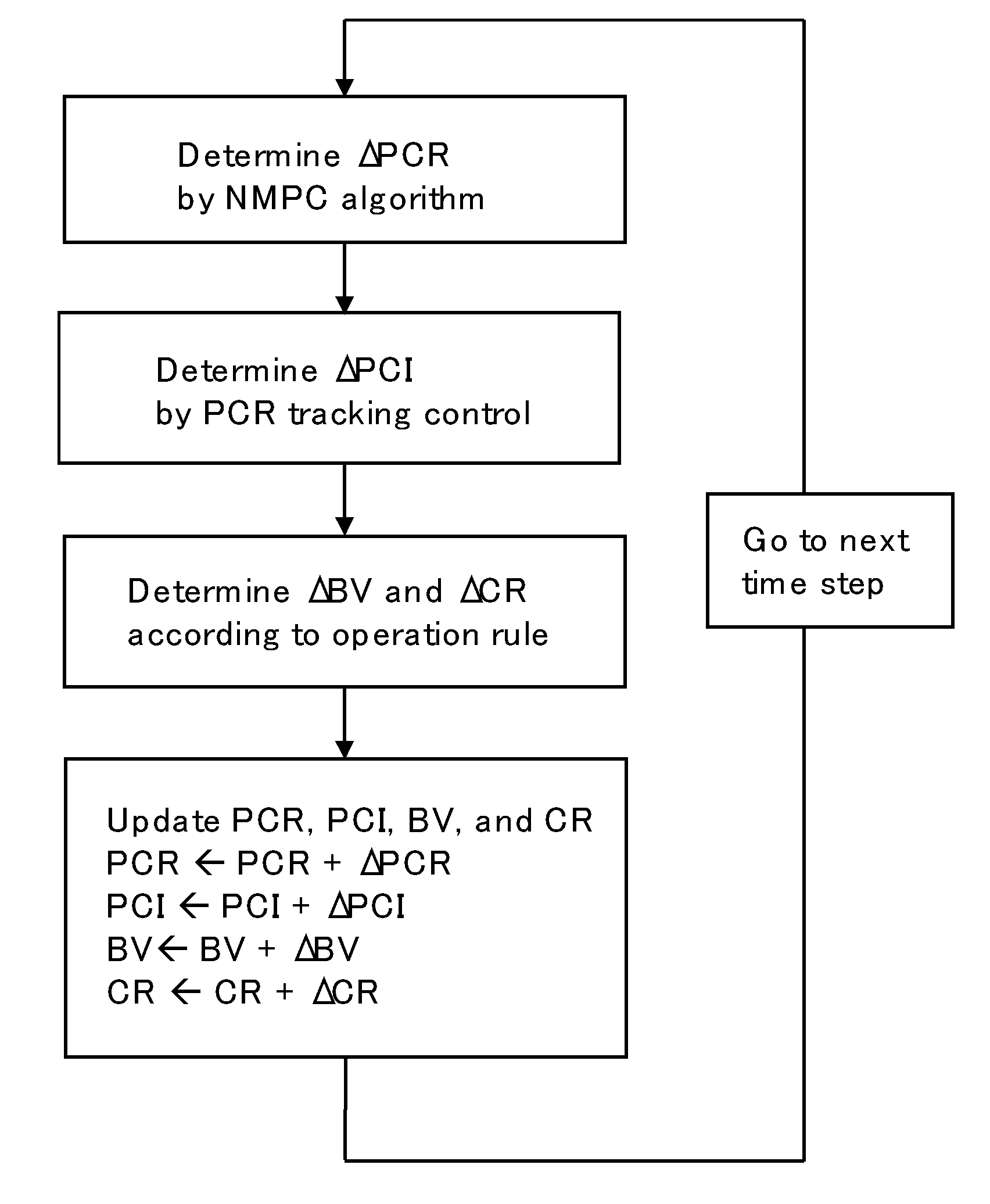
2.3. Nonlinear Model Predictive Control

This section describes the development of a control algorithm that derives the control actions similar to the current manual operation method in Section 2.1. First, the 2D transient model is represented in the form of a nonlinear state-space model.
x t + 1 = f x t , u t
y t = C x t
where x t denotes the state variables calculated in the 2D transient model, which includes the oxidation degree of iron and the temperatures of gas, coke, and iron. u t denotes the input variables listed in Table 1, expressed as u t = B V t , E O t , P C I t , B M t , B T t , C R t T . y t is the controlled variable, i.e., HMT, and is calculated by the function C , where the iron temperatures in the calculation cells at the tuyere height are averaged. The time step of the nonlinear state-space model was set to 15 min, because the measurement interval of HMT is about 30 min. To update the state variables by Equation (11), the 2D transient model calculation needs to be executed three times. This is because the time step of the 2D transient model is 5 min while that of the nonlinear state-space model is 15 min.
The outline of the NMPC algorithm is as follows. First, the free response of HMT is predicted assuming that the current input variables are kept constant at the current values. The step response of HMT when PCR is increased by a unit amount is then calculated. Finally, the optimal operation amount of the target PCR to maintain the HMT near the set point is calculated. To match the actual PCR with the target PCR, PI control is used to adjust the PC flow rate.
First, the free response y f t 0 + k is calculated by Equations (11) and (12) assuming that the input variables at the current time step t = t 0 are kept constant by fixing u t 0 + k = u t 0 . Considering the fact that it takes about eight hours for the material to descend through the furnace, k takes the values from 0 to 40 to predict up to ten-hour-ahead HMT. Figure 4 shows an example of the free response calculation. The origin of the horizontal axis is the moment when the prediction is performed. Figure 4a through f show the input variables of the 2D transient model, where the vertical axes are mean-centered. Figure 4g shows the free response of HMT by the blue solid line, where the vertical axis is the deviation from the set point. In this example, it is predicted that HMT decreases because CR is decreased at −15 h and−4 h.
The response of HMT when PCR is perturbed by Δ P C R 0 = 10   kg / t, i.e., y PCR t 0 + k , is then calculated. The operation of increasing PCR by Δ P C R 0 is denoted as Δ u 1 = 0 ,   0 , Δ P C I 0 ,   0 ,   0 ,   0 T , and y PCR t 0 + k is calculated by Equations (11) and (12), fixing u t 0 + k = u t 0 + Δ u 1 . The operation amount of the PC flow rate, i.e., Δ P C I 0 , was obtained by multiplying the current Prod and Δ P C R 0 . y PCR is indicated by the green dashed line in Figure 4g. The step response of HMT to the PCR manipulation was then extracted by subtracting y f from y PCR and dividing by Δ P C R 0 , as shown in Figure 4h.
S PCR k = y PCR t 0 + k y f t 0 + k / Δ P C R 0
The step response of HMT to the PCR manipulation starts to increase at 4 h. The reason for this dead time before HMT increases is as follows. The oxygen blown through the tuyeres is used to combust coke or PC in the raceway. Therefore, when the PC flow rate is increased under a constant oxygen flow rate, the coke combustion rate decreases. While PC is blown in at room temperature, coke is heated in the furnace and then combusted in the raceway. Hence, as the PC flow rate increases, the raceway gas temperature decreases due to the decrease in the combustion rate of hot coke. This decrease in the raceway gas temperature suppresses the increase of HMT for the first four hours.
The next step is to derive the optimal operation amount of PCR for controlling HMT. The future HMT was approximated by the linear combination of the free response and the step responses, which is shown by the blue line in the top row of Figure 5.
y p t 0 + k = y f t 0 + k + i = 0 T c S PCR k i θ i
where θ i is the operation amount of PCR at time step t 0 + i , which is the decision variable in the NMPC algorithm. A time series of θ i is indicated by the red arrows in the bottom row of Figure 5. Since the operators keep the target PCR to an integer value, the range of θ i was restricted to integers. T c is the control horizon, and it was set to 4 because the operators decide the control actions for the next one hour.
Since the operators tend to perform the minimum control actions necessary to achieve the control objective, the following evaluation function, which is indicated by the orange area in the top row of Figure 5, was designed.
J = k = T d T p α U k 2 + α L k 2
where T p is the prediction horizon, which was set to 40. T d corresponds to the dead time of the step response of HMT, which was set to 16. α U k + and α L k + are the amounts by which the future HMT is above the upper bound y U and below the lower bound y L , respectively.
y p t 0 + k y U + α U k
y p t 0 + k y L α L k  
y U and y L were set to the target HMT +5 °C and −5 °C, respectively.
In addition, constraints on the operation amount of the target PCR by one control action were also set.
θ i θ max δ i
θ i θ min δ i  
where θ max and θ min are the maximum and minimum operation amounts, which were set to 5 and 2, respectively. δ i 0 , 1 is the switch variable to keep or change the PCR. Using this switch variable, the operation amount is guaranteed to be more than θ min when the target PCR is changed.
As described above, under the constraints of Equations (16) through (19), the time series of θ i is determined by mixed integer quadratic programming (MIQP) so that the evaluation function J in Equation (15) is minimized. The optimal operation amount of PCR at the current time, Δ P C R opt , is the first element of the time series of θ i , that is, Δ P C R opt = θ 0 .
The PCR tracking control to calculate the operation amount of PC flow rate so that the actual PCR and the target PCR match is also described here. After Δ P C R opt is obtained by the NMPC algorithm, the operation amount of the PC flow rate is calculated by
Δ P C I opt = γ 0 δ P C R 0 + γ 1 δ P C R 0 δ P C R 1 + Δ P C R opt P r o d 0  
where δ P C R 0 and δ P C R 1 are the control deviation of PCR at the current time step and the previous time step, respectively. γ 0 and γ 1 are the relaxation coefficients. P r o d 0 is the production rate at the current time step.

3. Results and Discussion

This section presents the results of the validation of the NMPC algorithm. First, the control simulations are executed under the disturbance of changes in CR, BV, and EO. The automatic HMT control system using this control algorithm is then implemented in the actual furnace, and its effectiveness in reducing HMT variation is evaluated.

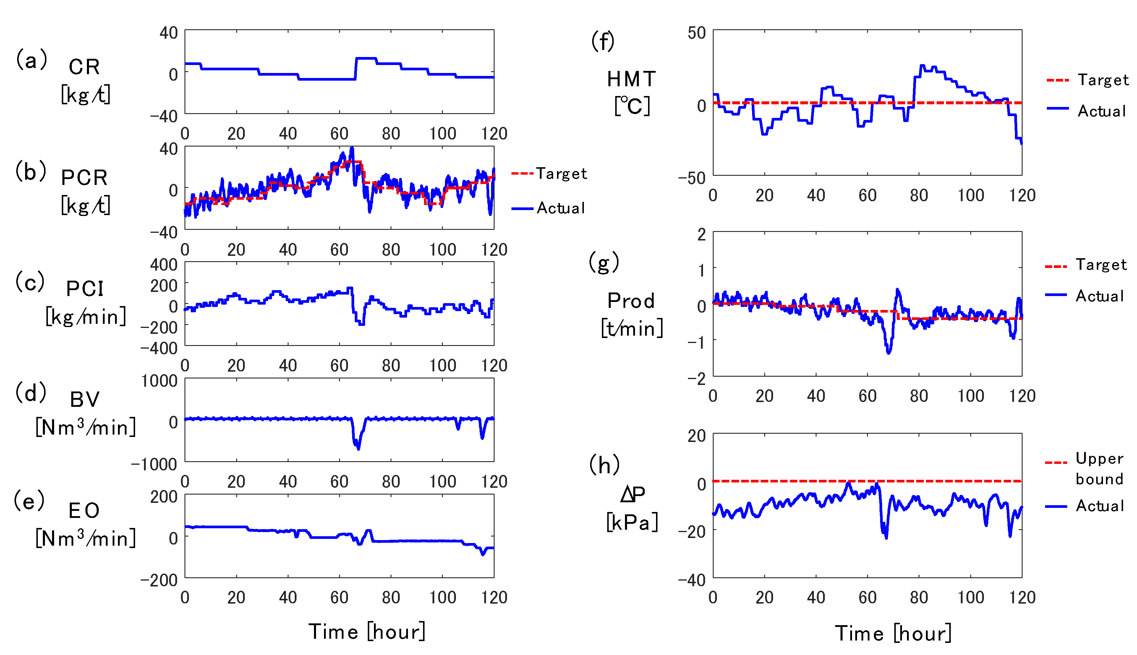
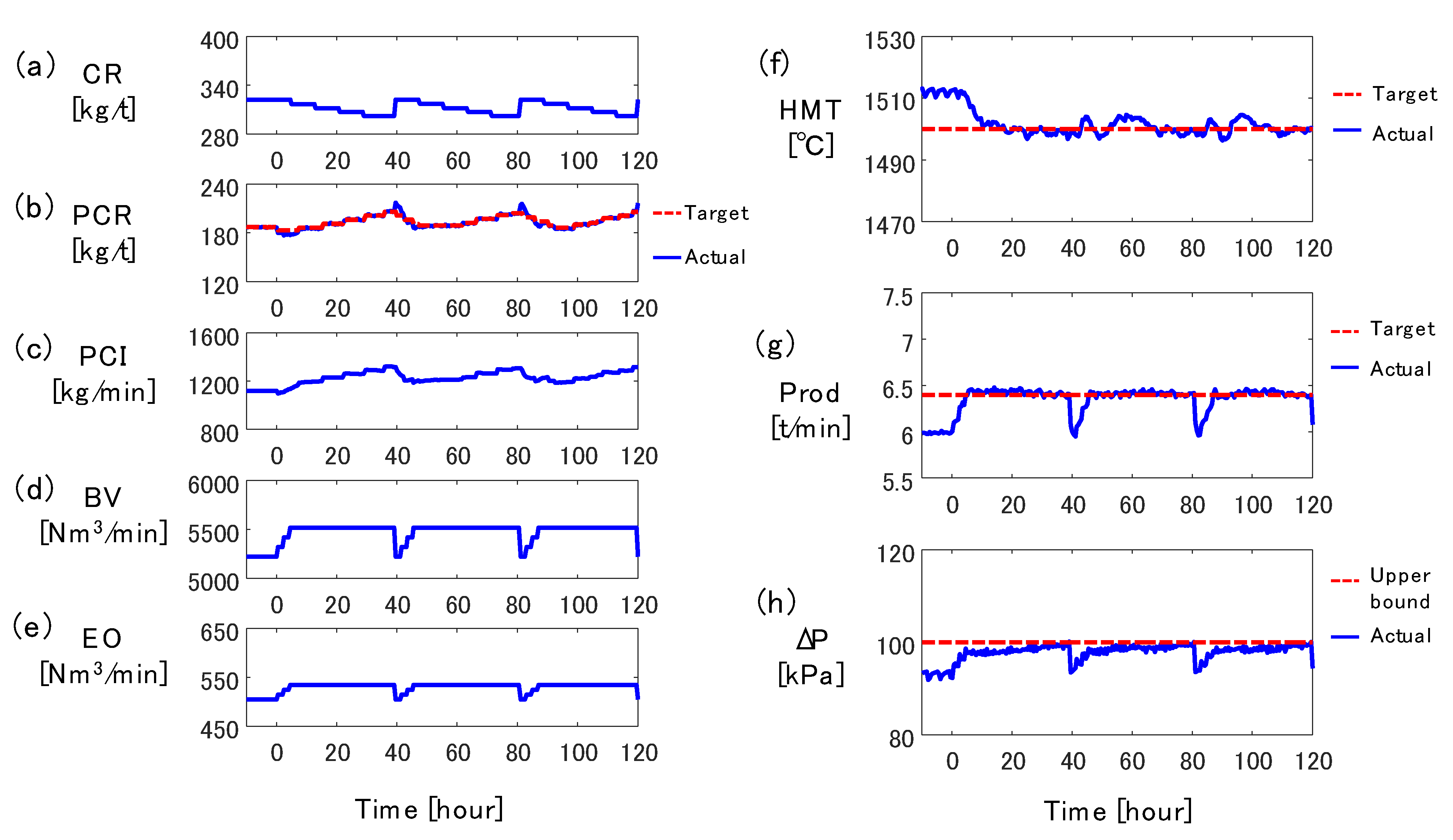
3.1. Control Simulation Results

In the conventional manual operation, the operators decrease CR gradually and manipulate BV and EO to achieve the target production rate as long as ΔP is below the upper bound, as shown in Figure 2. In addition, they increase CR and decrease BV simultaneously when ΔP exceeds the upper bound. The control simulations were carried out under this operation rule, the details of which are shown in Appendix A. Figure 6 shows the flowchart of the control simulation. The target PCR and PC flow rate are manipulated using the NMPC algorithm described in Section 2.3 to investigate whether the developed control algorithm can suppress the effects of disturbance due to the changes in CR and BV. For the simplicity of the simulation, EO was adjusted proportionately to BV. BM and BT were not manipulated in this simulation.
First, the input variables in Table 3 were fed to the 2D transient model until the periodic steady state was reached, and the NMPC algorithm was then activated. Figure 7 shows the results of the simulation, where the origin of the horizontal axis is the moment when the NMPC algorithm was activated. The left column shows the variables which can be manipulated, and the right column shows the outcomes of the operation, i.e., HMT, Prod, and ΔP. The Prod was calculated by substituting the estimates by the 2D transient model into Equations (2) and (3). The ΔP was obtained by subtracting the top gas pressure from the gas pressure at the height of tuyere.
An operational trend similar to that in Figure 2 was reproduced by the control simulation. According to the operation rule, CR was lowered gradually from 0 to 30 h, and it increased ΔP during the same period. BV and EO were also manipulated to achieve the target production rate. When ΔP reached the upper bound at 39 h, BV and EO were decreased and CR was increased. The CR was lowered and BV was increased again from 40 h to 78 h. To counteract these disturbances, the NMPC algorithm properly manipulated the target PCR to cancel the effect of the change in CR on HMT. For example, the target PCR was increased from 5 h to 36 h to compensate for the decrease of CR, and it was decreased rapidly around 40 h to suppress the effect of CR increase on HMT. The PCR tracking control appropriately manipulated the PC flow rate to match the actual PCR and the target PCR. As a result, HMT was maintained within the target value ±10 °C.

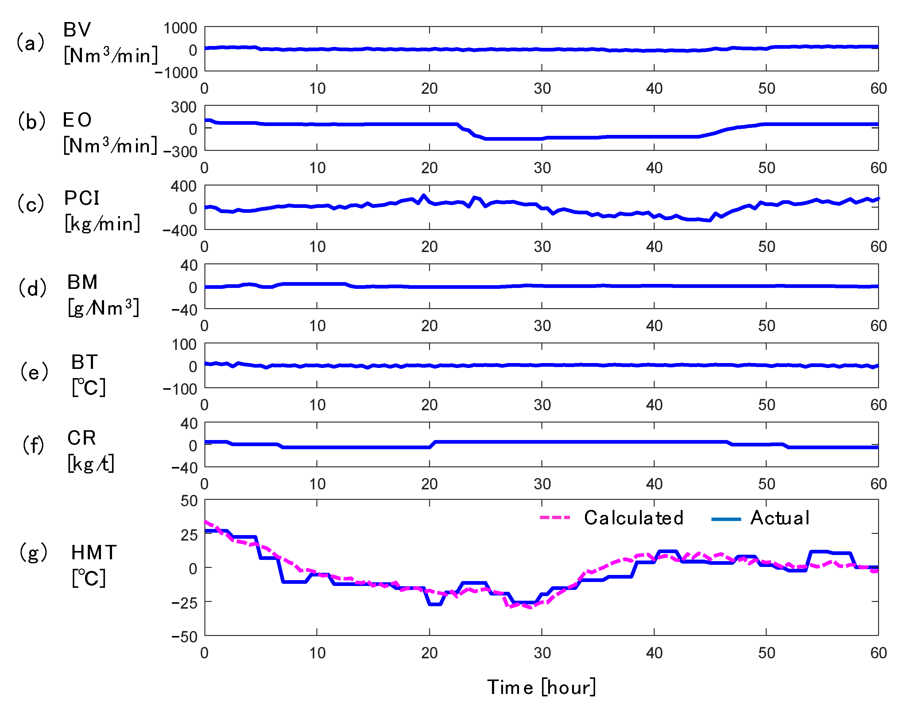
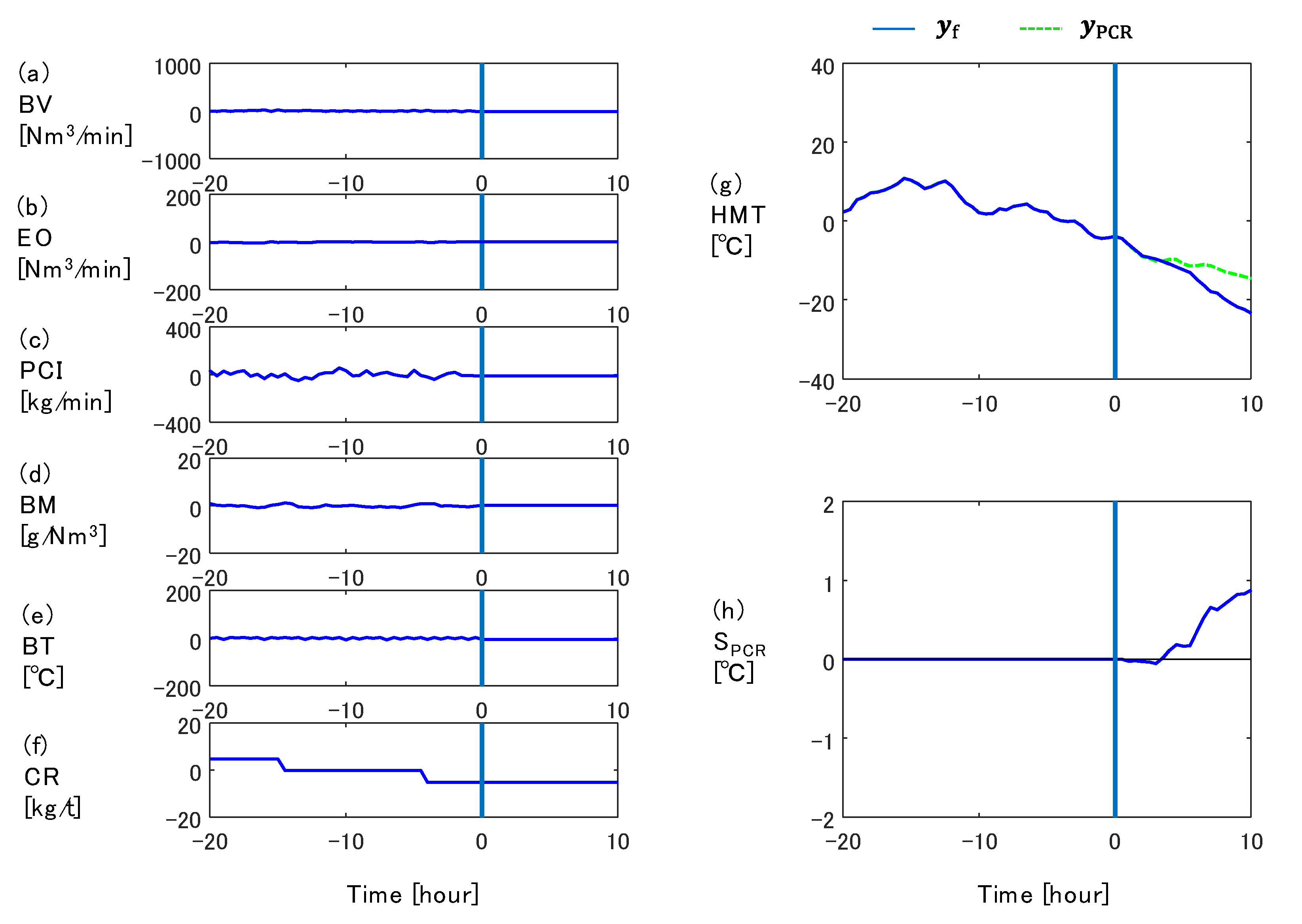
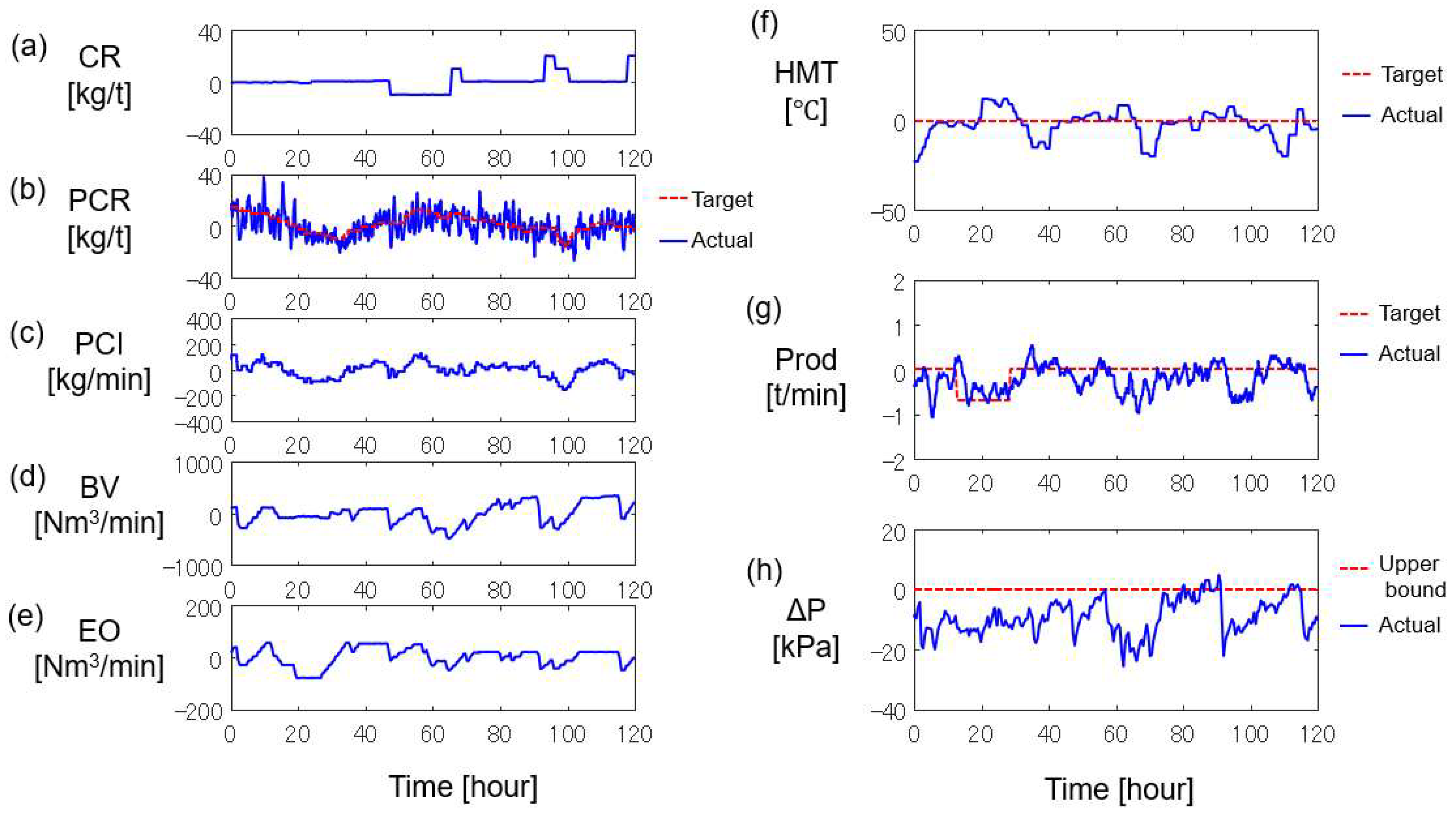
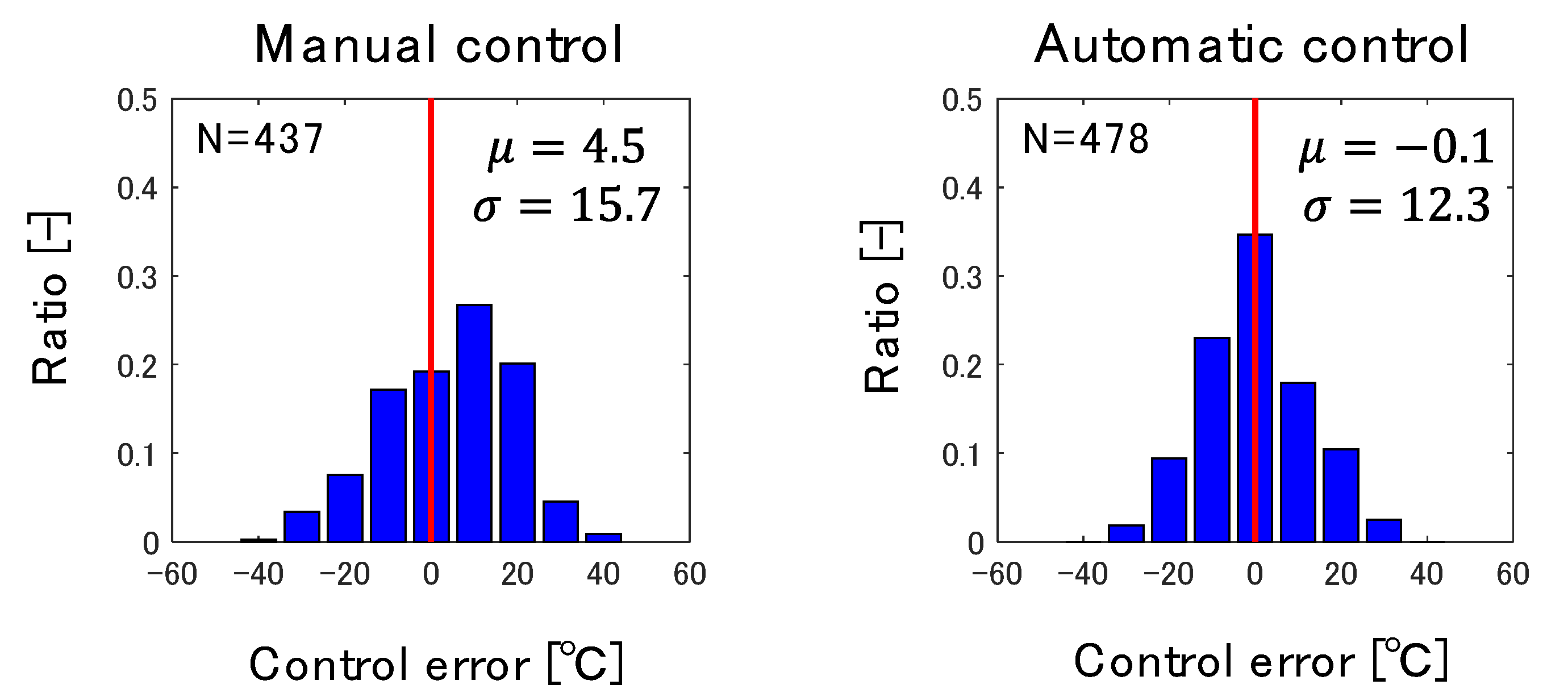
3.2. Evaluation in Actual Operation

An automatic control system based on the NMPC algorithm was implemented in the actual blast furnace. Figure 8 shows the operational trend for 120 h. The red dashed lines and blue solid lines represent the target value (or upper bound) and actual values, respectively. The manipulated variables by the control system are the target PCR and PC flow rate shown in Figure 8b,c. The other variables in the left column, i.e., CR, BV, and EO, were manipulated by the operators. The right column shows the results of the operation, i.e., HMT, Prod, and ΔP. The vertical axes in the left column are all mean-centered, whereas those in the right column show the difference from the target value (or upper bound) at time zero.
The operators manipulated BV and EO in response to the changes in target Prod at 10 h and 30 h. Since ΔP reached the upper limit at 55 h and 90 h, BV and EO were decreased, followed by the increase in CR. While ΔP was below the upper bound, BV and EO were manipulated to achieve the target Prod and CR was decreased to reduce the operating costs.
Despite the large changes in CR, BV, and EO, HMT was kept within the target value ±20 °C as shown in Figure 8f, because the developed control system appropriately manipulated the target PCR and the PC flow rate. For instance, the target PCR was increased by 20 kg/t at around 52 h to suppress the decrease in HMT due to the decrease of CR at 48 h. The target PCR was decreased by 20 kg/t around 96 h to cancel the effect of CR increase at 92 h. In addition, the target PCR and actual PCR were matched by appropriately manipulating the PC flow rate according to the decrease and increase in Prod due to changes in BV and EO from 92 h to 110 h.
Figure 9 shows a histogram of the deviation of HMT from its target before and after the introduction of the developed control system. Conventionally, the operators controlled HMT to a value higher than the target value to avoid operational risks due to an excessively low HMT, and consumption of excess reducing agent was an issue. The developed control system successfully reduced the root mean square (RMS) of the control error by 3.4 °C, and decreased the average control error by 4.6 °C without increasing the frequency of excessively low HMT, i.e., less than −30 °C. According to the step response calculation when the PC flow rate is increased, the increase in RAR by 1 kg/t increases HMT by approximately 2 °C at a steady state [9]. Hence, the reduction of the average control error of HMT by 4.6 °C leads to the decrease of RAR by 2.3 kg/t. This decrease in RAR reduces the amount of CO2 by 20 kt/y. Currently, the developed control system has been used continuously in the actual operation, but it is difficult to apply the control system to highly transient operating conditions such as during the transition period from stoppage to normal operation. The authors will further expand the range of applications of the developed control system by improving the accuracy of the 2D transient model in future work.

4. Conclusions

In this paper, a control algorithm using nonlinear model predictive control (NMPC) was developed to control hot metal temperature (HMT). Simulation verification under operating conditions simulating a real plant showed that the algorithm generates control actions of pulverized coal rate (PCR) similar to those by the operators and maintains HMT within the target value ±10 °C. Furthermore, the automatic control system based on this control algorithm was implemented in an actual plant. As a result, the developed control system suppressed the effects of disturbances of changes in the coke rate (CR) and blast volume (BV) and successfully reduced the average control error of HMT by 4.6 °C compared to the conventional manual operation. The developed control system has contributed to the reduction of RAR and CO2 emissions.

Author Contributions

Conceptualization, Y.H.; methodology, Y.H. and R.M.; software, Y.H. and R.M.; validation, Y.H.; investigation, Y.H.; writing—original draft preparation, Y.H.; writing—review and editing, Y.H.; supervision, M.M. and M.M.v.P. All authors have read and agreed to the published version of the manuscript.

Funding

This research received no external funding.

Data Availability Statement

Not applicable.

Conflicts of Interest

The authors declare no conflict of interest.

Nomenclature

B M Blast moistureg/Nm3
B T Blast temperature°C
B V Blast volumeNm3/min
C p Specific heatJ/kg/K
C R Coke ratekg/t
E Heat exchange coefficientW/m3/K
E O Enrichment oxygen flow rateNm3/min
m i , j Molar ratio of substance i in reaction j-
O ore Oxygen amount in unreduced iron orekmol/t
P g Gas pressurePa
P C I Pulverized coal flow ratekg/min
P C R Pulverized coal ratekg/t
P r o d Production ratet/min
q Heat-loss through furnace wallW/m2
R Reaction ratekmol/m3/sec
R g Gas generation ratekg/m3/sec
S PCR Step response of HMT to PCR°C/(kg/t)
T Temperature°C
u Input variables-
u fe Molar velocity of ironkmol/m2/sec
u g Mass velocity of gaskg/m2/sec
u g 0 Molar velocity of gaskmol/m2/sec
V in O Amount of oxygen blown into furnacekmol/min
V out O Amount of oxygen in top gaskmol/min
V top Top gas flow ratekmol/min
x State variable-
X 1 X 5 Molar ratio of gas component
1: N2, 2: CO, 3: CO2, 4: H2, 5: H2O
-
X 6 X 9 Mol fraction of iron component
6: O (contained in FeOx), 7: [C], 8: [Si], 9: H2O (liq)
-
X c Volume ratio of cokem3-coke/m3-bed
X o Volume ratio of orem3-ore/m3-bed
X ϕ Volume ratio of gas component ϕ -
y Controlled variable-
α Control error of HMT°C
γ Relaxation coefficient of PCR tracking control-
δ Switch variable-
Δ H R Reaction heatJ/kmol
Δ P Pressure dropPa
Δ P C I Operation amount of PC flow ratekg/min
δ P C R Control error of PCRkg/t
Δ P C R Operation amount of target PCRkg/t
η Distribution ratio of reaction heat-
θ Decision variable in MIQPkg/t
ρ c Apparent density of cokekg/m3-coke
ρ fe Iron density in sintered iron orekmol/m3-ore
ρ g Density of gaskg/m3

Appendix A

The details of the operation rule are explained here. As long as ΔP is below the upper bound, BV was manipulated so that the actual Prod matched the target Prod. The operation amount of BV was fixed to Δ B V 0 = 100   Nm 3 / min . CR is lowered by Δ C R 0 = 5   kg / t to reduce the operating costs.
Δ B V = Δ B V 0 * sign max P r o d t 0 P r o d U , 0 + min P r o d t 0 P r o d L , 0  
Δ C R = Δ C R 0
where P r o d t 0 is the estimated Prod at the current time step, and P r o d U and P r o d L are the upper bound and lower bound of Prod which were set to the target Prod + 0.05 t/min and—0.05 t/min, respectively.
When ΔP is above the upper bound, BV is decreased by Δ B V 1 = 300   Nm 3 / min and CR is increased by Δ C R 1 = 20   kg / t to decrease ΔP.
Δ B V = Δ B V 1 ,     Δ C R = + Δ C R 1
The interval of control actions was restricted to 2 h for BV manipulation and 8 h for CR manipulation, regardless of ΔP.

References

  1. Iffat, U.; Bhatia, S.; Tantar, A.; Sanz, J.; Schockaert, C.; Schimitz, A.; Ciroldini, F.; Reuter, Y.; Hansen, F. New digital services for manufacturing industry using analytics: The case of blast furnace thermal regulation. In Proceedings of the 2018 IEEE 20th Conference on Business Informatics (CBI), Vienna, Austria, 11–14 July 2018; pp. 89–91. [Google Scholar]
  2. Spirin, N.A.; Lavrov, V.V.; Rybolovlev, V.Y.; Schnaider, D.A.; Krasnobaev, A.V.; Gurin, I.A. Digital Transformation of Pyrometallurgical Technologies. State, Scientific Problems, and Prospects of Development. Steel Transl. 2021, 51, 522–530. [Google Scholar] [CrossRef]
  3. Azadi, P.; Winz, J.; Leo, E.; Klock, R.; Engell, S. A hybrid dynamic model for the prediction of molten iron and slag quality indices of a large-scale blast furnace. Comput. Chem. Eng. 2022, 156, 107573. [Google Scholar] [CrossRef]
  4. Jiang, K.; Jiang, Z.; Xie, Y.; Chen, Z.; Pan, D.; Gui, W. Classification of silicon content variation trend based on fusion of multilevel features in blast furnace ironmaking. Inf. Sci. 2020, 521, 32–45. [Google Scholar] [CrossRef]
  5. Agrawal, A.; Agarwal, M.K.; Kothari, A.K.; Mallick, S. A mathematical model to control thermal stability of blast furnace using proactive thermal indicator. Ironmak. Steelmak. 2019, 46, 133–140. [Google Scholar] [CrossRef]
  6. Martín, R.D.; Obeso, F.; Mochón, J.; Barea, R.; Jiménez, J. Hot metal temperature prediction in blast furnace using advanced model based on fuzzy logic tools. Ironmak. Steelmak. 2007, 34, 241–247. [Google Scholar] [CrossRef]
  7. Jiao, H.; Zhang, Y.; Luo, C.; Bi, Z. Collaborative Multiple Rank Regression for Temperature Prediction of Blast Furnace. IEEE Trans. Instrum. Meas. 2022, 71, 3515110. [Google Scholar] [CrossRef]
  8. Hashimoto, Y.; Sawa, Y.; Kano, M. Practical Operation Guidance on Thermal Control of Blast Furnace. ISIJ Int. 2019, 59, 1573–1581. [Google Scholar] [CrossRef]
  9. Hashimoto, Y.; Kitamura, Y.; Ohashi, T.; Sawa, Y.; Kano, M. Transient model-based operation guidance on blast furnace. Control Eng. Pract. 2019, 82, 130–141. [Google Scholar] [CrossRef]
  10. Hashimoto, Y.; Sawa, Y.; Kano, M. Online Prediction of Hot Metal Temperature Using Transient Model and Moving Horizon Estimation. ISIJ Int. 2019, 59, 1534–1544. [Google Scholar] [CrossRef]
  11. Hashimoto, Y.; Masuda, R.; Yasuhara, S. An Operator Behavior Model for Thermal Control of Blast Furnace. ISIJ Int. 2022, 62, 157–164. [Google Scholar] [CrossRef]
  12. Abhale, P.B.; Viswanathan, N.N.; Saxén, H. Numerical modelling of blast furnace –Evolution and recent trends. Miner. Process. Extr. Metall. 2020, 129, 166–183. [Google Scholar] [CrossRef]
  13. Saxén, H. Blast furnace on-line simulation model. Metall. Mater. Trans. B 1990, 21, 913–923. [Google Scholar] [CrossRef]
  14. Fu, D.; Chen, Y.; Zhao, Y.; Alessio, J.D.; Ferron, K.J.; Zhou, C.Q. CFD modeling of multiphase reacting flow in blast furnace shaft with layered burden. Appl. Therm. Eng. 2014, 66, 298–308. [Google Scholar] [CrossRef]
  15. Castro, J.A.; Nogami, H.; Yagi, J. Transient Mathematical Model of Blast Furnace Based on Multi-fluid Concept, with Application to High PCI Operation. ISIJ Int. 2000, 40, 637–646. [Google Scholar] [CrossRef]
  16. Hashimoto, Y.; Sawa, Y.; Kano, M. Development and Validation of kinematical blast furnace model with long-term operation data. ISIJ Int. 2018, 58, 2210–2218. [Google Scholar] [CrossRef]
  17. Jiao, L.; Kuang, S.; Yu, A.; Li, Y.; Mao, X.; Xu, H. Three-Dimensional Modeling of an Ironmaking Blast Furnace with a Layered Cohesive Zone. Metall. Mater. Trans. B 2020, 51, 258–275. [Google Scholar] [CrossRef]
Figure 1. Overview of blast furnace process.
Metals 12 01624 g001
Figure 2. Example of manual operation of blast furnace: (a) coke rate, (b) pulverized coal rate, (c) PC flow rate, (d) blast volume, (e) enrichment oxygen flow rate, (f) hot metal temperature, (g) production rate, (h) pressure drop.
Metals 12 01624 g002
Figure 3. Simulation results of HMT by 2D transient model using real operation data: (a) blast volume, (b) enrichment oxygen flow rate, (c) PC flow rate, (d) blast moisture, (e) blast temperature, (f) coke rate, (g) hot metal temperature.
Metals 12 01624 g003
Figure 4. Calculation of free response and step response of HMT: (a) blast volume, (b) enrichment oxygen flow rate, (c) PC flow rate, (d) blast moisture, (e) blast temperature, (f) coke rate, (g) hot metal temperature, (h) step response of HMT to PCR.
Metals 12 01624 g004
Figure 5. Decision variable and evaluation function in NMPC algorithm.
Metals 12 01624 g005
Figure 6. Flowchart of control simulation.
Metals 12 01624 g006
Figure 7. Control simulation result: (a) coke rate, (b) pulverized coal rate, (c) PC flow rate, (d) blast volume, (e) enrichment oxygen flow rate, (f) hot metal temperature, (g) production rate, (h) pressure drop.
Metals 12 01624 g007
Figure 8. Real operation result by developed control system: (a) coke rate, (b) pulverized coal rate, (c) PC flow rate, (d) blast volume, (e) enrichment oxygen flow rate, (f) hot metal temperature, (g) production rate, (h) pressure drop.
Metals 12 01624 g008
Figure 9. Improvement of HMT control accuracy by automatic control.
Metals 12 01624 g009
Table 1. Classification of variables in this work.
CategoryVariableUnit
Input variables for
simulation
Blast volume (BV)Nm3/min
Enrichment oxygen flow rate (EO)Nm3/min
Blast moisture (BM)g/Nm3
Blast temperature (BT)°C
Pulverized coal flow rate (PCI)kg/min
Coke rate (CR), i.e., weight ratio of coke and ironkg/t
Manipulated variables for controlPulverized coal rate (PCR)kg/t
Pulverized coal flow rate (PCI)kg/min
Controlled variableHot metal temperature (HMT)°C
Table 2. Reactions in the 2D transient model.
SymbolReaction
R 1 FeO x + CO = FeO x 1 + CO 2
R 2 C + CO 2 = 2 CO
R 3 FeO + C = Fe + CO
R 4 FeO x + H 2 = FeO x 1 + H 2 O
R 5 C + H 2 O = CO + H 2
R 6 CO + H 2 O = CO 2 + H 2
R 7 C coke = C
R 8 SiO 2 + 2 C = Si + 2 CO
R 9 H 2 O l = H 2 O g
R 10 C + 1 / 2 O 2 = CO   raceway
R 11 C + H 2 O = CO + H 2 raceway
Table 3. Standard operation condition used in control simulation.
Input VariablesValue
Blast volume (BV)5200 Nm3/min
Enrichment oxygen flow rate (EO)500 Nm3/min
Blast moisture (BM)7 g/Nm3
Blast temperature (BT)1130 °C
Pulverized coal flow rate (PCI)1120 kg/min
Coke rate (CR)332 kg/t
Publisher’s Note: MDPI stays neutral with regard to jurisdictional claims in published maps and institutional affiliations.

