Denoising and Dehazing an Image in a Cascaded Pattern for Continuous Casting

Abstract

Automatic vision systems have been widely used in the continuous casting of the steel industry, which improve efficiency and reduce labor. At present, high temperatures with evaporating fog cause images to be noisy and hazy, impeding the usage of advanced machine learning algorithms in this task. Instead of considering denoising and dehazing separately like previous papers, we established that by taking advantage of deep learning in a modeling complex formulation, our proposed algorithm, called Cascaded Denoising and Dehazing Net (CDDNet) reduces noise and hazy in a cascading pattern. Experimental results on both synthesized images and a pragmatic video from a continuous casting factory demonstrate our method’s superior performance in various metrics. Compared with existing methods, CDDNet achieved a 50% improvement in terms of peak signal-to-noise ratio on the validation dataset, and a nearly 5% improvement on a dataset that has never seen before. Besides, our model generalizes so well that processing a video from an operating continuous casting factory with CDDNet resulted in high visual quality.

1. Introduction

Computer vision has seen remarkable progress in the domains of image classification [1,2,3,4], semantic segmentation [5,6,7], and restoration from degradation [8,9,10,11]. There is no doubt that traditional industries seek to obtain advantages in terms of safety and efficiency with the assistance of computer vision. However, since production environments require high robustness and stability, deploying advanced but tricky algorithms to these industries is questionable. For example, in the continuous casting of the steel industry, due to its inevitably high-temperature environment, imaging suffers from noise and haze, leading to low visual quality. Figure 1 shows an example from a real continuous casting factory. The bottom area of the ladle (blue area in Figure 1) is where the vision system focuses on in order to drive the robot arms (red area in Figure 1) to install the long casting nozzle, but both the areas captured by the camera are deteriorated highly by haze and noise due to the high temperature. High-level computer vision tasks, such as detection and recognition, may fail in this situation. Considering that noise and haze misleading the computer vision algorithm prevent the development of vision system advances in the continuous casting of steel, it is crucial and fundamental for vision systems that are pursuing robustness and accuracy to denoise and dehaze at an early stage.

In this paper, we propose a high performance end-to-end denoising and dehazing convolutional nerual network (CNN) model, called Cascaded Denoising and Dehazing Net (CDDNet). While some approaches either neglect the influence of image noise or reduce noise separately, CDDNet is designed to be a two-stage end-to-end pipeline which removes noise and haze in a cascading pattern. It was trained on synthesized hazy and noisy images, and was tested on synthetic images and a real video from an in-operation continuous casting factory. Experiments demonstrated that CDDNet performs well. It is exciting to share that our proposed model generalizes so well that a real video processed by CDDNet result in high visual quality.

To summarize, our contributions include:

• We analyze the atmospheric scattering model and additive noise from the perspective of combining them. We further expand this formula into a new denoising and dehazing algorithm that works in a cascading pattern.
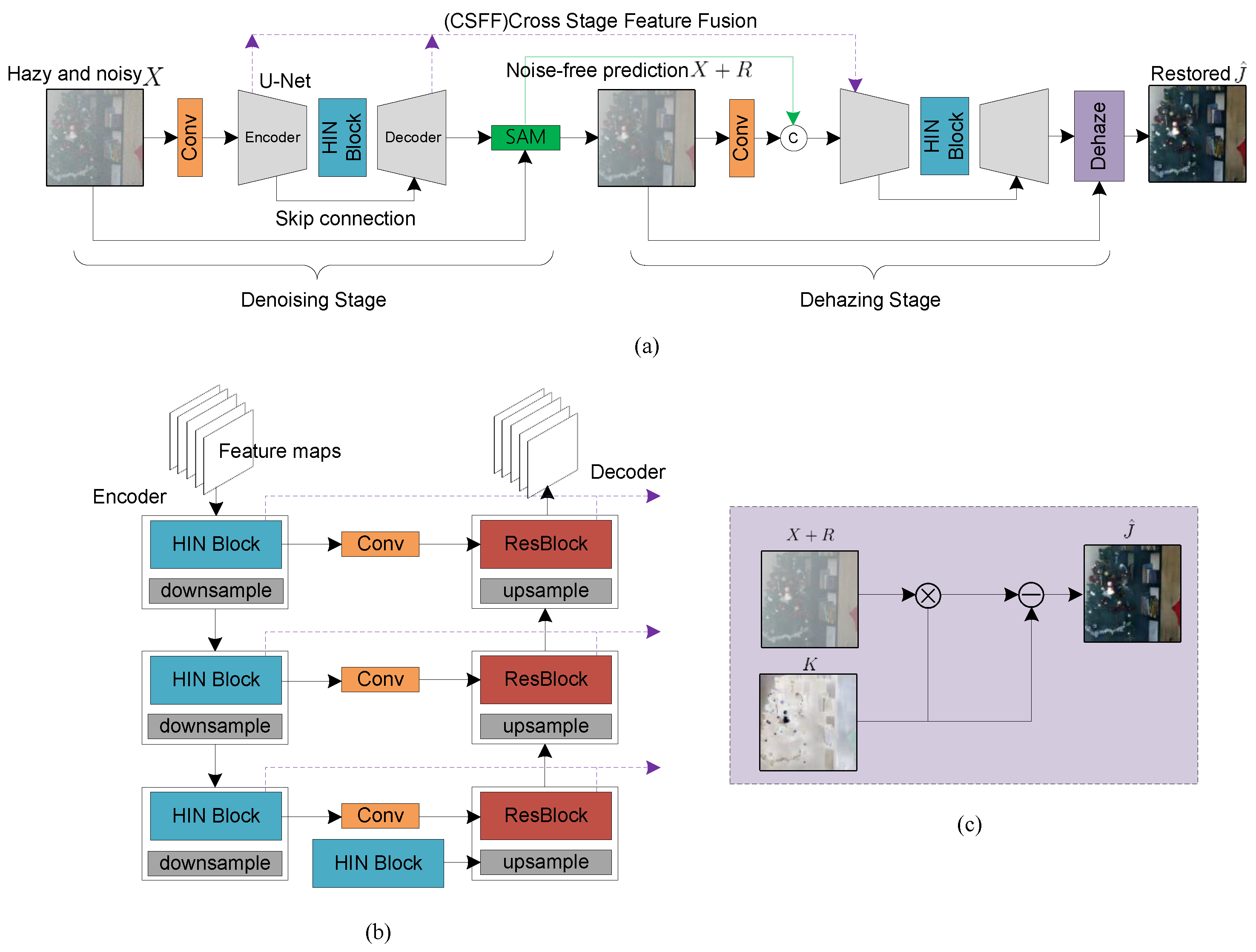
• We propose CDDNet, a cascading two-stage U-Net for image denoising and dehazing.
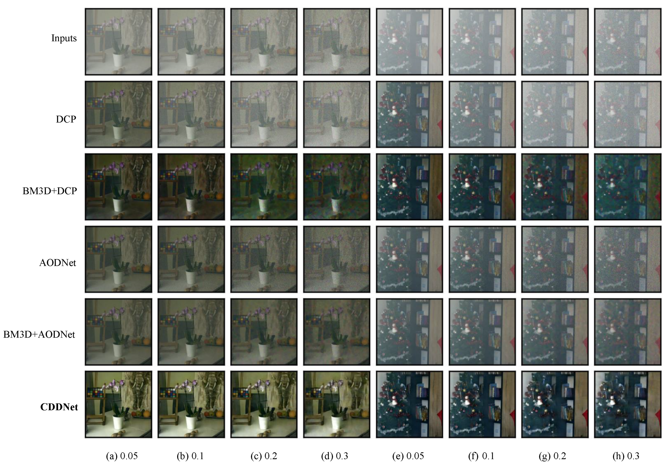
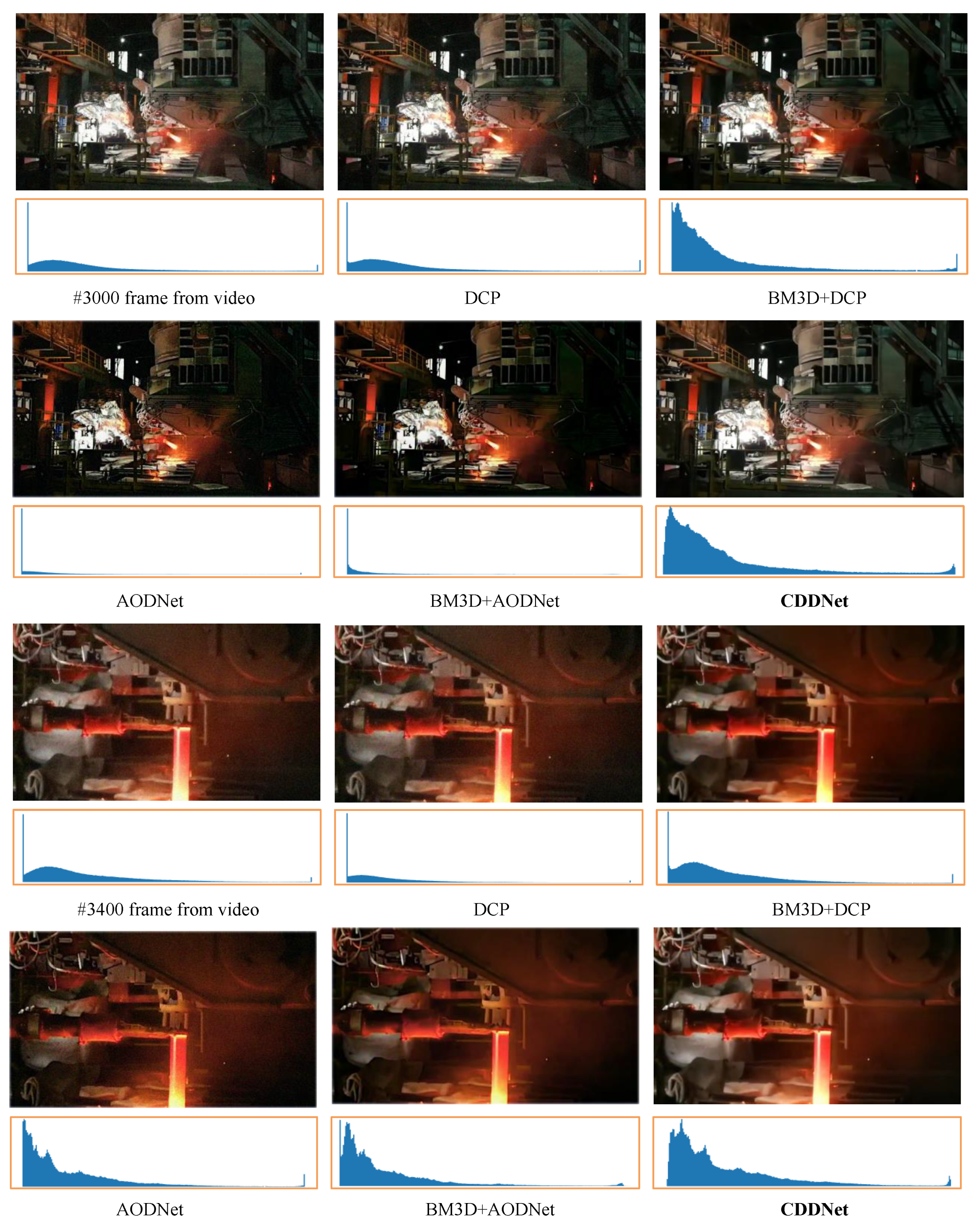
• We provide in-depth experiments on both synthesized images and a real video from a continuous casting factory, which demonstrates that CDDNet achieves superior performance to other models.

2. Related Work

The continuous casting of the steel industry inevitably occurs in high temperature environments with a lack of ambient light. When placing industrial cameras in such situations, these disadvantages lead to image degradation in two ways. First, the camera is unable to gain enough photons to activate; meanwhile, electric signals on the sensor tend to be unstable and leak out. Both factors result in significant noise. Second, the high temperature in this environment leads to much evaporation and liquefaction, generating haze which considerably obscures the targets being watched. In this section, we first overview the basic models of haze and additive noise that are of essential importance to CDDNet’s design.

In computer vision, the formation of hazy images is usually described by the atmospheric scattering model [12,13,14]:

$$I\left(x\right)=J\left(x\right)t\left(x\right)+A(1-t(x\left)\right),$$

(1)

where $I\left(x\right)$ is observed hazy image and $J\left(x\right)$ is the clean image to be recovered. There are two parameters that need to be figured out: A denotes the global atmospheric light, and $t\left(x\right)$ is the transmission matrix defined as:

$$t\left(x\right)=e^{-\beta d\left(x\right)},$$

(2)

where $\beta$ is the scattering coefficient of the atmosphere, and $d\left(x\right)$ is the distance from the target to the camera. The goal of image dehazing is to recover the $J\left(x\right)$ from the $I\left(x\right)$.

In recent years, there has been significant progress in image haze removal, and these methods tend to take priors or make assumptions about the hazy images. By observing that hazy images have lower contrast than clean images, Tan et al. [15] aimed to enlarge the local contrast to improve the visibility of hazy images. However, since different images have very different parameters of haze, editing contrast arbitrarily brings out fidelity loss. He [16] observed that the Dark Channel Prior (DCP) reliably calculates the transmission matrix, but the DCP fails when objects share a similar color to the atmospheric light A as a result of the transmission value tending to be zero. Zhu et al. [17] proposed a color attenuation prior to recover images, and the model parameters were learned in a supervised way. Since the success of convolutional neural networks in image processing, numerous related algorithms based on CNN have emerged. DehazeNet proposed by Cai et al. [18] is a CNN-based network elaborately trained to predict a transmission matrix, and the global atmospheric light is estimated by empirical rules. All-in-One Net transforms the atmospheric scattering model into a unified model, and dehazes images directly without estimating A and $t\left(x\right)$ [10].

When considering image noise, the main challenge is to recover a clean image x from the noisy observation y, with the additive noise n, namely:

$$y=x+n.$$

(3)

Most of these denoising methods can be classified into three groups: (1) based on the assumption of local similarity of image methods, (2) transforming domain methods, and (3) convolutional neural network methods. The first group of denoising methods searches the local window of the image and restores the pixels according to similar parts of the image. Non-Local Mean (NLM)) proposed by Buades et al. [19], and Block-matching and 3D filtering (BM3D) proposed by Dabov et al. [20] are the two most successful representatives of the first group. Since noise and signal usually exhibit different frequency spectra, Portilla et al. [21] utilized the sparsity of the image in the transformed domain. Deep learning methods have the advantage of fitting a complex distribution, and are becoming promising techniques for denoising. NBNet proposed by Cheng et al. [8], and MemNet porposed by Tai et al. [22] are CNN-based methods that have superior denosing performance. However, in the steel industry, pure denosing is insufficient, since the vast majority of interference cases come from haze.

All above methods either cope with haze or noise; however, Matlin et al. [23] showed that the noise will be amplified if we only process the haze. Denoising is vital, since the image noise is everywhere, especially in a high-temperature environment such as that of continuous casting areas in the steel industry. Liu et al. [24] observed that the haze almost completely resides in the low frequencies, while noisy tends to have higher frequencies. It is obvious to decompose the image into frequency domains and then filter these disadvantages and reconstruct from the frequency domain. However, textures and edges in images are inevitably smoothed, and extra detail enhancement tricks are utilized to compensate for the loss of information.

In conclusion, dehazing and denoising have the features of ubiquity and being ill-posed. The methods described above all ignore one of the two problems because they do not address pragmatic industry scenarios or split haze and noise into different domains under the naive assumption of no coupling. Our work not only deals with the dehazing and denosing synchronously, but also uses no other prior about the relationship between haze and noise: we came up with an end-to-end, CNN-based solution with superior performance.

3. Method

In this section, the proposed CDDNet is explained; see Figure 2a. CDDNet splits the restoration process into two steps (denosing and dehazing) in a cascading pattern in order to remove noise and haze synchronously. The rest of this section is structured as follows: first, we combine the atmospheric scattering model and additive noise, leading to a more complex yet pragmatic form. Second, our proposed method, CDDNet, inspired by the complex formula, is explained in detail.

3.1. Transformed Formula

According to Section 2, we are not only concerned about the haze, but also the additive noise:

$$I\left(x\right)=J\left(x\right)t\left(x\right)+A(1-t(x\left)\right)+n\left(x\right),$$

(4)

where I is the observed image degraded by both haze and additive noise, and n is the noise contribution, assumed to be independent and identically distributed, with zero mean and variance ${\sigma }^2$. Matlin et al. [23] proved that if an image is preprocessed only by dehaze algorithms, the noise level of the image will be amplified exponentially. In order to avoid the amplifying, we split the restoration process into two stages in a cascading pattern by first denoisiong the image, and then following a dehazing procedure. During the first stage, the noise is treated as an additive term that can be removed by fitting its mean and variance, for which a neural network does a good job. After the first stage, we obtain

$$I\left(x\right)-\widehat{n}\left(x\right)=Y\left(x\right)=J\left(x\right)t\left(x\right)+A(1-t\left(x\right)),$$

(5)

where $\widehat{n}$ is the estimated noise term, and Y is the denoising restoration. The noise-free image is then transferred to the second stage for dehazing. During the second stage, similarly to AODNet, we unify the two parameters t and A into one formula, i.e., K in Equation (6),

$$\begin{array}{cc}\hfill J\left(x\right)& \hfill =K\left(x\right)I\left(x\right)-K\left(x\right)+b,\mathrm{where}\hfill \\ \hfill K\left(x\right)& \hfill =\frac{\frac{1}{t\left(x\right)}(I\left(x\right)-A)+(A-b)}{I\left(x\right)-1},\hfill \end{array}$$

(6)

where $K\left(x\right)$ is a integrated parameter unifying the global atmospheric light A and transmission matrix $t\left(x\right)$. b is a constant bias with a default value 1. The clean image $J\left(x\right)$ can be retrieved by Equation (6) once the unified parameter K is estimated.

3.2. CDDNet

The architecture of our proposed method, Cascaded Denoise and Dehaze Net (CDDNet), is shown in Figure 2a. CDDNet consists of two subnetworks, each of which is a U-Net. U-Net, proposed by Ronneberger et al. [5], is a popular baseline network especially adept at pixelwise dense prediction (the input is a whole image and the output is a whole image too). Each U-Net consists of two significant phases called encoder and decoder, as shown in Figure 2b.

In the encoder, U-Net, level by level, extracts different scales’ features while the spatial size of the input degraded image scales down. We replaced the regular extractor with a Half-Instance Normalization Block (HIN Block), since the HIN Block proposed by Chen et al. [9] achieves a balance between deep feature extraction and feature stability. We use five HIN Blocks concatenated to form the encoding phase, and four convolution blocks with a kernel size of 4 each between HIN Blocks to downsample the feature maps.

In the decoder, U-Net utilizes and rescales the information-rich features from the encoding phase to recover the image, level by level. Similarly to HINet proposed by Chen et al. [9], we use four ResBlocks to extract high-level features, and four transpose convolution blocks, each of which is between ResBlocks, to upsample the features. Pixelwise prediction tasks, such as image restoration and semantic segmentation, are faced with the difficulty that when digging into higher-level features for gaining a deeper understanding of an image, a network designed with numerous extractors tends to, by inference, produce a low-resolution result. One of the reasons why U-Net is all the rage is that the skip connection fuses features from the encoder component to compensate for the loss of information caused by resampling, which leads to a high-resolution result. We also adopt the skip connection in order to get a high-resolution restoration.

The first subnetwork of CDDNet takes the degraded image with noise and haze as input X and generates a noise estimation R. The supervised attention module proposed by Mehri et al. [11] is deployed to generate the noise-free image by $X+R$ according to Equation (5) and to connect the second subnetwork of CDDNet in a cascading pattern. The latter stage receives a noise-free estimation from the previous stage and produces the estimation of parameter K. At last, the dehazing module combines K and noise-free estimation, as shown in Figure 2c, to generate a haze-free result $\widehat{J}$. We also allow some kinds of information exchange between these two subnetworks by using cross-stage feature fusion [11].

4. Experiments

We evaluated our approach on a wide range of datasets and report the standard metrics, including PSNR and SSIM. The datasets, brief introductions of metrics, and training details are as follows.

4.1. Implementation Details

Datasets We first created synthetic hazy images from the NYU2 Dataset [25] by setting different atmospheric light levels and scattering coefficients. We took 27,000 synthetic hazy images as training dataset and the rest images as TestSet A. We randomly added Gaussian noise (zero mean and standard deviation varying from 0.01 to 0.3) to the hazy image, then synthesized a set of images with haze and additive noise. Besides synthetic hazy images, we took I-HAZE [26] as TestSet B, a dataset that contains 35 image pairs of hazy and corresponding haze-free indoor images. Hazy images were generated using real haze produced by a professional haze machine. In addition, we also collected a real video (TestSet C) from an in-operation continuous casting factory, which truly causes image noise and haze.

Metrics We use peak signal-to-noise ratio (PSNR) and structural similarity index measure (SSIM) to quantify the restoration performance. PSNR refers to the ratio between the maximum possible power of a signal and the power of corrupting noise that affects the fidelity of its representation [27]. In the filed of image processing, given a noise-free image (groundtruth)I and its estimation K, PSNR is defined as:

$$\begin{array}{cc}\hfill \mathrm{PSNR}& \hfill =10\times {\log }_{10}({\mathrm{MAX}}_I^2/\left(\frac{1}{mn}\sum _{i=0}^{m-1}\sum _{j=0}^{n-1}{[I(i,j)-K(i,j)]}^2\right)),\hfill \end{array}$$

(7)

where I is of size $m\times n$ and ${\mathrm{MAX}}_I$ is the maximum possible pixel value of the image. The higher PSNR is, the higher the quality of the restoration image. While PSNR is used for estimating absolute errors between the ground trth and the restoration, SSIM is used for measuring the structural similarity between two images [28]. SSIM is defined as:

$$SSIM(I,K)=\frac{\left(2{\mu }_I{\mu }_K+c_1\right)\left(2{\sigma }_{IK}+c_2\right)}{\left({\mu }_I^2+{\mu }_K^2+c_1\right)\left({\sigma }_I^2+{\sigma }_K^2+c_2\right)},$$

(8)

where $\mu$ is the average of the image, ${\sigma }^2$ denotes the variance of the image, ${\sigma }_{IK}$ is the covariance of two images, and $c_1,c_2$ are two variables to stabilize the division with a weak denominator. The higher SSIM is, the more faithful human perception is.

Training We used vanilla Stochastic Gradient Descent (SGD) with momentum 0.9 as the optimizer instead of Adam [29], since the adaptive optimization methods can be sensitive and exhibit poor generalization if the training set is noisy [30]. The learning rate was set to $2\times {10}^{-4}$ initially and decreased to $1\times {10}^{-6}$ with the cosine annealing strategy [31]. We first center cropped the training set from $640\times 480$ image resolution to $256\times 256$, and we trained CDDNet on these patches with a batch size of 32 for 100 epochs. Since CDDNet is a two-stage model including two inputs and outputs, we used two peak signal-to-noise ratio functions as the metrics of loss, PSNR loss. $X\in {\mathbb{R}}^{N\times C\times H\times W}$ denotes the input of first stage, where N is the batch size of data, C is the number of channels, and H and W are the spatial dimensions of the image. $R\in {\mathbb{R}}^{N\times C\times H\times W}$ denotes the inference of first stage, which is a noise estimation. $Y\in {\mathbb{R}}^{N\times C\times H\times W}$ denotes the ground truth image only degraded by haze. $K\in {\mathbb{R}}^{N\times C\times H\times W}$ is the final product of stage two, and $J\in {\mathbb{R}}^{N\times C\times H\times W}$ is the ground truth without noise and haze. Then CDDNet is optimized end-to-end by:

$$\mathit{Loss}=-\mathit{PSNR}(\underset{\mathrm{denoising}\mathrm{stage}}{\underbrace{X+R}},Y)-\mathit{PSNR}(\underset{\mathrm{dehazing}\mathrm{stage}}{\underbrace{K\times (X+R)-K+1}},J).$$

(9)

4.2. Quantitative Results

Most of the dehazing algorithms cannot handle the degradation caused by noise. As mentioned in Section 3, dehazing approaches that ignore noise will significantly amplify noise. Matlin et al. [23] suggests that combining denoise methods with dehazing methods will remit this problem. Thus, we compare CDDNet with pure dehazing methods: All-in-One Net proposed by Li et al. [10] and Dark-Channel Prior proposed by He et al. [16]. Meanwhile, we combined the denoising method BM3D with these dehazing methods to make a comprehensive comparison.

Table 1. PSNR and SSIM results of different methods under various noise levels with standard deviation varying among $\{0.05,0.1,0.2,0.3\}$.

Model	TestSet A				TestSet B
	0.05	0.1	0.2	0.3	0.05	0.1	0.2	0.3
DCP	$\genfrac{}{}{0pt}{}{18.08\mathrm{dB}}{\left(0.38\right)}$	$\genfrac{}{}{0pt}{}{16.28\mathrm{dB}}{\left(0.23\right)}$	$\genfrac{}{}{0pt}{}{13.10\mathrm{dB}}{\left(0.12\right)}$	$\genfrac{}{}{0pt}{}{10.88\mathrm{dB}}{\left(0.08\right)}$	$\genfrac{}{}{0pt}{}{14.40\mathrm{dB}}{\left(0.16\right)}$	$\genfrac{}{}{0pt}{}{12.97\mathrm{dB}}{\left(0.08\right)}$	$\genfrac{}{}{0pt}{}{10.58\mathrm{dB}}{\left(0.038\right)}$	$\genfrac{}{}{0pt}{}{9.10\mathrm{dB}}{\left(0.023\right)}$
AODNet	$\genfrac{}{}{0pt}{}{15.86\mathrm{dB}}{\left(0.34\right)}$	$\genfrac{}{}{0pt}{}{14.12\mathrm{dB}}{\left(0.20\right)}$	$\genfrac{}{}{0pt}{}{11.34\mathrm{dB}}{\left(0.10\right)}$	$\genfrac{}{}{0pt}{}{9.60\mathrm{dB}}{\left(0.07\right)}$	$\genfrac{}{}{0pt}{}{13.88\mathrm{dB}}{\left(0.16\right)}$	$\genfrac{}{}{0pt}{}{12.41\mathrm{dB}}{\left(0.07\right)}$	$\genfrac{}{}{0pt}{}{10.06\mathrm{dB}}{\left(0.029\right)}$	$\genfrac{}{}{0pt}{}{8.62\mathrm{dB}}{\left(0.0017\right)}$
BM3D + DCP	$\genfrac{}{}{0pt}{}{16.96\mathrm{dB}}{\left(0.77\right)}$	$\genfrac{}{}{0pt}{}{16.47\mathrm{dB}}{\left(0.71\right)}$	$\genfrac{}{}{0pt}{}{15.45\mathrm{dB}}{\left(0.63\right)}$	$\genfrac{}{}{0pt}{}{14.06\mathrm{dB}}{\left(0.56\right)}$	$\genfrac{}{}{0pt}{}{12.83\mathrm{dB}}{\left(0.58\right)}$	$\genfrac{}{}{0pt}{}{12.77\mathrm{dB}}{\left(0.56\right)}$	$\genfrac{}{}{0pt}{}{12.69\mathrm{dB}}{\left(0.52\right)}$	$\genfrac{}{}{0pt}{}{12.42\mathrm{dB}}{\left(0.49\right)}$
BM3D + AODNet	$\genfrac{}{}{0pt}{}{16.76\mathrm{dB}}{\left(0.76\right)}$	$\genfrac{}{}{0pt}{}{16.55\mathrm{dB}}{\left(0.71\right)}$	$\genfrac{}{}{0pt}{}{15.86\mathrm{dB}}{\left(0.65\right)}$	$\genfrac{}{}{0pt}{}{14.96\mathrm{dB}}{\left(0.60\right)}$	$\genfrac{}{}{0pt}{}{14.64\mathrm{dB}}{\left(0.66\right)}$	$\genfrac{}{}{0pt}{}{14.57\mathrm{dB}}{\left(0.64\right)}$	$\genfrac{}{}{0pt}{}{14.36\mathrm{dB}}{\left(0.61\right)}$	$\genfrac{}{}{0pt}{}{14.05\mathrm{dB}}{\left(0.5\right)}$
CDDNet	$\genfrac{}{}{0pt}{}{25.37\mathrm{dB}}{\left(0.89\right)}$	$\genfrac{}{}{0pt}{}{24.65\mathrm{dB}}{\left(0.86\right)}$	$\genfrac{}{}{0pt}{}{23.61\mathrm{dB}}{\left(0.81\right)}$	$\genfrac{}{}{0pt}{}{22.87\mathrm{dB}}{\left(0.78\right)}$	$\genfrac{}{}{0pt}{}{15.33\mathrm{dB}}{\left(0.724\right)}$	$\genfrac{}{}{0pt}{}{15.23\mathrm{dB}}{\left(0.70\right)}$	$\genfrac{}{}{0pt}{}{15.01\mathrm{dB}}{\left(0.67\right)}$	$\genfrac{}{}{0pt}{}{14.69\mathrm{dB}}{\left(0.64\right)}$
	$\genfrac{}{}{0pt}{}{\uparrow 7.29\mathrm{dB}}{(0.12)}$	$\genfrac{}{}{0pt}{}{\uparrow 8.1\mathrm{dB}}{\left(0.15\right)}$	$\genfrac{}{}{0pt}{}{\uparrow 7.75\mathrm{dB}}{\left(0.16\right)}$	$\genfrac{}{}{0pt}{}{\uparrow 7.91\mathrm{dB}}{\left(0.18\right)}$	$\genfrac{}{}{0pt}{}{\uparrow 0.69\mathrm{dB}}{\left(0.064\right)}$	$\genfrac{}{}{0pt}{}{\uparrow 0.66\mathrm{dB}}{\left(0.06\right)}$	$\genfrac{}{}{0pt}{}{\uparrow 0.65\mathrm{dB}}{\left(0.06\right)}$	$\genfrac{}{}{0pt}{}{\uparrow 0.64\mathrm{dB}}{\left(0.14\right)}$
$\genfrac{}{}{0pt}{}{\mathrm{PSNR}}{\mathrm{improvements}}$	$\uparrow 40.3\%$	$\uparrow 48.9\%$	$\uparrow 48.9\%$	$\uparrow 52.9\%$	$\uparrow 4.7\%$	$\uparrow 4.5\%$	$\uparrow 4.5\%$	$\uparrow 4.6\%$

shows the average PSNR and SSIM results on TestSets A and B with $\sigma \in \{0.05,0.1,0.2,0.3\}$, respectively. Since CDDNet was validated on TestSets A, it made sense for it to obtain superior scores in terms of PSNR and SSIM on this dataset. TestSet B is a challenge for deep learning methods like CDDNet and AODNet, because these methods have never seen TestSet B before and the results mostly show how well the deep learning methods generalize. Compared with BM3D+AODNet on TestSet B, the PSNR and SSIM of CDDNet increased by 0.66 dB and 0.08, on average. These results prove that CDDNet generalizes and performs better than BM3D + AODNet. The last two rows of Table 1 show the differences (improvements) between CDDNet’s scores and the corresponding best scores of the other methods. We conclude that CDDNet obtained superior PSNR and SSIM performance to all competitors under a variety of challenging circumstances.

Figure 3 displays part of the visual results from TestSet B. The second (DCP) and fourth (AODNet) rows of Figure 3 reveal that pure dehazing methods reduced haze from a global perspective, leading to the contrast of the image widening. The dehazing performance of these traditional methods decayed as $\sigma$ increased. As can be seen from the third (BM3D+DCP) and fifth (BM3D+AODNet) rows of Figure 3, denosing before dehazing resulted in better visual quality. For example, in the fourth (Figure 3d) and eighth (Figure 3h) column ($\sigma =0.3$), it can be seen that BM3D+DCP could further clean the rest of the haze that vanilla DCP could not. However, BM3D inevitably blurred the origin while denosing, leaving an artistic result. CDDNet, in the last row of Figure 3, obtained high visual quality results compared with the other methods. We conclude that our method can retrieve clean images from severely deteriorated images.

4.3. Visual Results and Discussion

We collected a real video (TestSet C) from an in-operation continuous casting factory that truly suffers from image noise and haze. We again evaluated TestSet C with CDDNet and the methods compared above. Figure 4 demonstrates frames 3000 and 3400 from the video being restored by the methods mentioned above. Each of the restoration images has a histogram figure below that was used for judging the entire tonal distribution of a digital image. The more the histogram shows the full range of intensities evenly, the higher the global contrast of the image. Low-contrast images tend to be either too bright or too dark, causing rich details and textures to be invisible. As can be seen from Figure 4, the raw frames are hazy and noisy, and have low global contrast (most of the data points distribute on the left side of the histogram). The methods mentioned above have few positive effects on histogram distribution. AODNet and BM3D + AODNet tended to set numerous pixel values to zero, causing the result to be too dark. For example, there are still some details at the right bottom area of frame 3000, but AODNet made this area invisible. CDDNet not only restored the image from its hazy and noisy state, but also spread the histogram distribution, leaving appropriate contrast. We can see the brightest part of image (the red hot long casting nozzle), besides the darkest details, taken the right bottom part of frame 3000, for example.

We also analyze some regions of interest in Figure 5. As is shown, pure dehazing methods (first and third columns) amplify the noise and bring about even more degradation. Combining with denosing approaches, these dehazing methods converge but tend to lose fine details. For instance, the second row of Figure 5 is an electric wire. CDDNet retained fine details as much as possible, whereas other methods blurred the region and caused some pixel overflow (red and green points). The last row is a region where dense and bright white haze obscures the background. The BM3D + methods were confused by the light, resulting in incorrect color restoration (white mixed with rainbow colors). CDDNet not only made the background equipment appear, but also kept the colors accurate.

5. Conclusions

In this paper, by deciding to gather additive noise with an atmospheric scattering model, we proposed CDDNet, a two-stage convolutional network that reduces haze and noise in a cascading pattern. We compared CDDNet with a variey of methods, on synthetic images and a video (we collected it from an in-operation continuous casting factory), using both objective metrics (PSNR, SSIM) and histogram distributions. Extensive experimental results show that, when being faced with haze and noise, CDDNet achieves superior performance in dehazing and denoising, and restores the images to a high visual standard. Since few restoration methods were designed especially for the continuous casting of the steel industry, we were excited to witness that our proposal has promising generalization to a real continuous casting environment.

References

1. Krizhevsky, A.; Sutskever, I.; Hinton, G.E. ImageNet Classification with Deep Convolutional Neural Networks. In Advances in Neural Information Processing Systems; Pereira, F., Burges, C.J.C., Bottou, L., Weinberger, K.Q., Eds.; Curran Associates, Inc.: New York, NY, USA, 2012; Volume 25. [Google Scholar]
2. Szegedy, C.; Liu, W.; Jia, Y.; Sermanet, P.; Reed, S.; Anguelov, D.; Erhan, D.; Vanhoucke, V.; Rabinovich, A. Going Deeper with Convolutions. In Proceedings of the IEEE Conference on Computer Vision and Pattern Recognition, Boston, MA, USA, 7–12 June 2014. [Google Scholar]
3. He, K.; Zhang, X.; Ren, S.; Sun, J. Deep Residual Learning for Image Recognition. In Proceedings of the IEEE Conference on Computer Vision and Pattern Recognition, Las Vegas, NV, USA, 27–30 June 2016. [Google Scholar]
4. Wang, H.; Huang, R.; Gao, L.; Wang, W.; Xu, A.; Yuan, F. Wear Debris Classification of Steel Production Equipment using Feature Fusion and Case-based Reasoning. ISIJ Int. 2018, 58, 1293–1299. [Google Scholar] [CrossRef]
5. Ronneberger, O.; Fischer, P.; Brox, T. U-Net: Convolutional Networks for Biomedical Image Segmentation. In Proceedings of the International Conference on Medical Image Computing and Computer-Assisted Intervention, Munich, Germany, 5–9 October 2015. [Google Scholar]
6. Long, J.; Shelhamer, E.; Darrell, T. Fully Convolutional Networks for Semantic Segmentation. In Proceedings of the IEEE Conference on Computer Vision and Pattern Recognition, Boston, MA, USA, 7–12 June 2015. [Google Scholar]
7. He, K.; Gkioxari, G.; Dollár, P.; Girshick, R. Mask R-CNN. In Proceedings of the IEEE International Conference on Computer Vision (ICCV), Venice, Italy, 22–29 October 2017. [Google Scholar]
8. Cheng, S.; Wang, Y.; Huang, H.; Liu, D.; Fan, H.; Liu, S. NBNet: Noise Basis Learning for Image Denoising with Subspace Projection. In Proceedings of the Proceedings of the IEEE/CVF Conference on Computer Vision and Pattern Recognition, Nashville, TN, USA, 19–25 June 2021. [Google Scholar]
9. Chen, L.; Lu, X.; Zhang, J.; Chu, X.; Chen, C. HINet: Half Instance Normalization Network for Image Restoration. In Proceedings of the IEEE/CVF Conference on Computer Vision and Pattern Recognition, Nashville, TN, USA, 19–25 June 2021. [Google Scholar]
10. Li, B.; Peng, X.; Wang, Z.; Xu, J.; Feng, D. AOD-Net: All-in-One Dehazing Network. In Proceedings of the 2017 IEEE International Conference on Computer Vision (ICCV), Venice, Italy, 22–29 October 2017; pp. 4780–4788. [Google Scholar] [CrossRef]
11. Mehri, A.; Ardakani, P.B.; Sappa, A.D. MPRNet: Multi-Path Residual Network for Lightweight Image Super Resolution. In Proceedings of the IEEE/CVF Winter Conference on Applications of Computer Vision, Waikola, HI, USA, 5–9 January 2021. [Google Scholar]
12. Cox, L. Optics of the Atmosphere-Scattering by Molecules and Particles. Opt. Acta Int. J. Opt. 1977, 24, 779. [Google Scholar] [CrossRef]
13. Narasimhan, S.; Nayar, S. Chromatic framework for vision in bad weather. In Proceedings of the IEEE Conference on Computer Vision and Pattern Recognition. CVPR 2000 (Cat. No.PR00662), Hilton Head Island, SC, USA, 15 June 2000; Volume 1, pp. 598–605. [Google Scholar] [CrossRef] [Green Version]
14. Narasimhan, S.; Nayar, S. Vision and the Atmosphere. In International Journal of Computer Vision; Springer: Berlin/Heidelberg, Germany, 2002; pp. 233–254. [Google Scholar] [CrossRef]
15. Tan, R.T. Visibility in bad weather from a single image. In Proceedings of the 2008 IEEE Conference on Computer Vision and Pattern Recognition, Anchorage, AK, USA, 24–26 June 2008; pp. 1–8. [Google Scholar] [CrossRef]
16. He, K.; Sun, J.; Tang, X. Single image haze removal using dark channel prior. In Proceedings of the 2009 IEEE Conference on Computer Vision and Pattern Recognition, Miami, FL, USA, 22–24 June 2009; pp. 1956–1963. [Google Scholar] [CrossRef]
17. Zhu, Q.; Mai, J.; Shao, L. A Fast Single Image Haze Removal Algorithm Using Color Attenuation Prior. IEEE Trans. Image Process. 2015, 24, 3522–3533. [Google Scholar] [PubMed] [Green Version]
18. Cai, B.; Xu, X.; Jia, K.; Qing, C.; Tao, D. DehazeNet: An End-to-End System for Single Image Haze Removal. IEEE Trans. Image Process. 2016, 25, 5187–5198. [Google Scholar] [CrossRef] [PubMed] [Green Version]
19. Buades, A.; Coll, B.; Morel, J.M. Non-Local Means Denoising. Image Process. OnLine 2011, 1, 208–212. [Google Scholar] [CrossRef] [Green Version]
20. Dabov, K.; Foi, A.; Katkovnik, V.; Egiazarian, K. Image Denoising by Sparse 3-D Transform-Domain Collaborative Filtering. IEEE Trans. Image Process. 2007, 16, 2080–2095. [Google Scholar] [CrossRef] [PubMed]
21. Portilla, J.; Strela, V.; Wainwright, M.; Simoncelli, E. Image denoising using scale mixtures of Gaussians in the wavelet domain. IEEE Trans. Image Process. 2003, 12, 1338–1351. [Google Scholar] [CrossRef] [PubMed] [Green Version]
22. Tai, Y.; Yang, J.; Liu, X.; Xu, C. MemNet: A Persistent Memory Network for Image Restoration. In Proceedings of the IEEE International Conference on Computer Vision (ICCV), Venice, Italy, 22–29 October 2017. [Google Scholar]
23. Matlin, E.; Milanfar, P. Removal of Haze and Noise from a Single Image; Electronic Imaging; International Society for Optics and Photonics: Bellingham, WA, USA, 2012. [Google Scholar]
24. Liu, X.; Zhang, H.; Cheung, Y.M.; You, X.; Tang, Y.Y. Efficient single image dehazing and denoising: An efficient multi-scale correlated wavelet approach. Comput. Vis. Image Underst. 2017, 162, 23–33. [Google Scholar] [CrossRef]
25. Silberman, N.; Hoiem, D.; Kohli, P.; Fergus, R. Indoor Segmentation and Support Inference from RGBD Images. In Proceedings of the European Conference on Computer Vision, Florence, Italy, 7–13 October 2012. [Google Scholar]
26. Ancuti, C.O.; Ancuti, C.; Timofte, R.; Vleeschouwer, C.D. I-HAZE: A dehazing benchmark with real hazy and haze-free indoor images. arXiv 2018, arXiv:1804.05091v1. [Google Scholar]
27. Wikipedia Contributors. Peak Signal-to-Noise Ratio—Wikipedia, The Free Encyclopedia. Available online: https://en.wikipedia.org/wiki/Peak_signal-to-noise_ratio (accessed on 5 January 2022).
28. Wikipedia Contributors. Structural Similarity—Wikipedia, The Free Encyclopedia. Available online: https://en.wikipedia.org/wiki/Structural_similarity (accessed on 5 January 2022).
29. Kingma, D.P.; Ba, J. Adam: A Method for Stochastic Optimization. 2017. Available online: http://xxx.lanl.gov/abs/1412.6980 (accessed on 5 January 2022).
30. Chaudhury, S.; Yamasaki, T. Robustness of Adaptive Neural Network Optimization Under Training Noise. IEEE Access 2021, 9, 37039–37053. [Google Scholar] [CrossRef]
31. Loshchilov, I.; Hutter, F. SGDR: Stochastic Gradient Descent with Warm Restarts. arXiv 2017, arXiv:cs.LG/1608.03983. [Google Scholar]
Figure 1. Any vision system in the continuous casting of the steel industry suffers from noise and haze. (a) A frame from a continuous casting factory. (b,c) Showing that haze and noise lead to low visual quality.
Metals 12 00126 g001
Figure 2. Network architecture and its components. (a) Overall CDDNet architecture. (b) U-Net with the CSFF module. We only show three layers for simplicity. (c) Dehazing module.
Metals 12 00126 g002
Figure 3. Challenging real hazy images from I-HAZE addressed with various methods.
Metals 12 00126 g003
Figure 4. Hazy and noisy frames from video. CDDNet restores images with high visual qulity.
Metals 12 00126 g004
Figure 5. Hazy and noisy frames from a video. CDDNet retained fine details and kept the colors accurate.
Metals 12 00126 g005