
Finite Element Analysis of the Magnetic Field Distribution in a Magnetic Abrasive Finishing Station and its Impact on the Effects of Finishing Stainless Steel AISI 304L


Abstract
1. Introduction
2. Materials and Methods
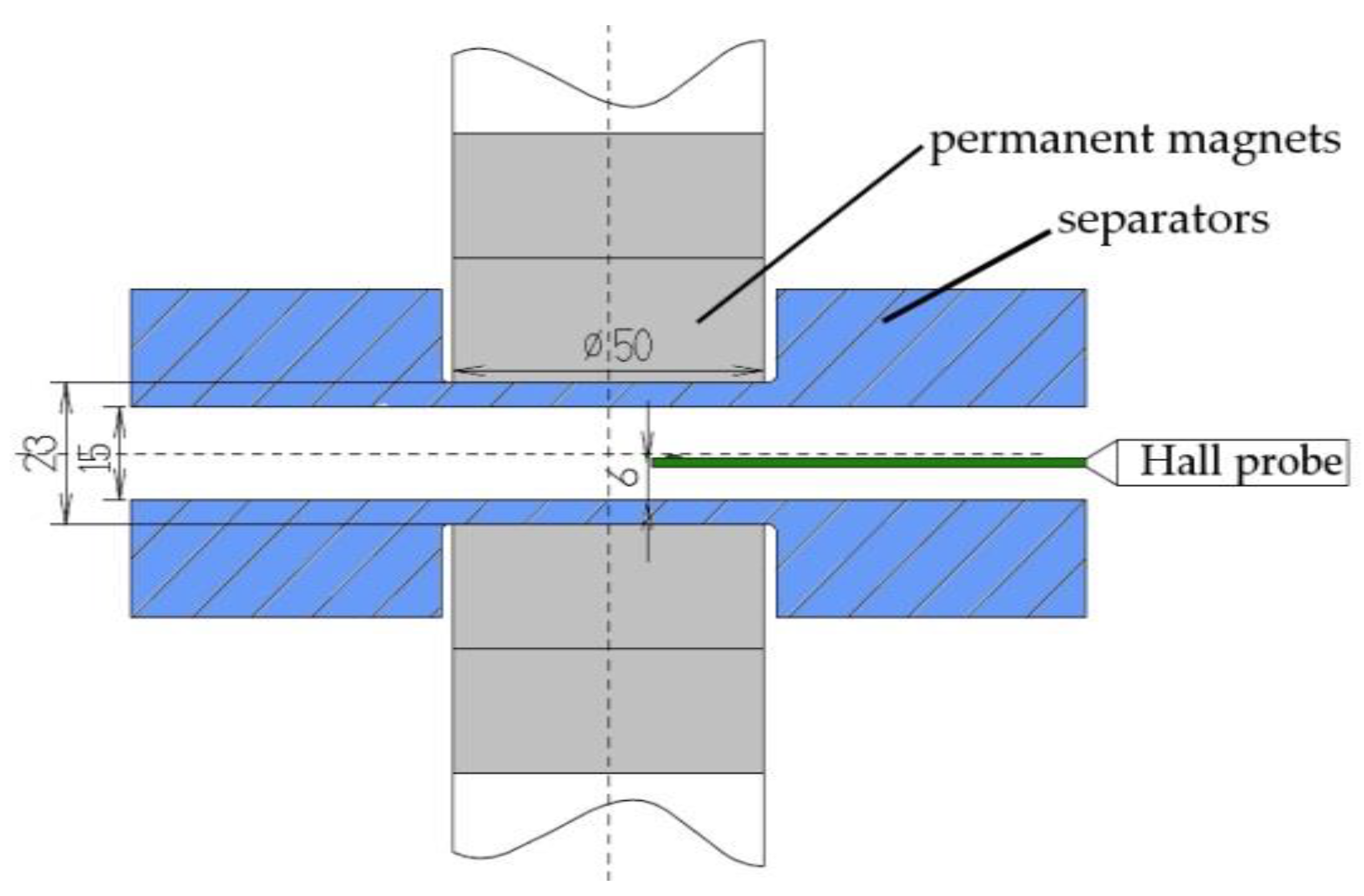
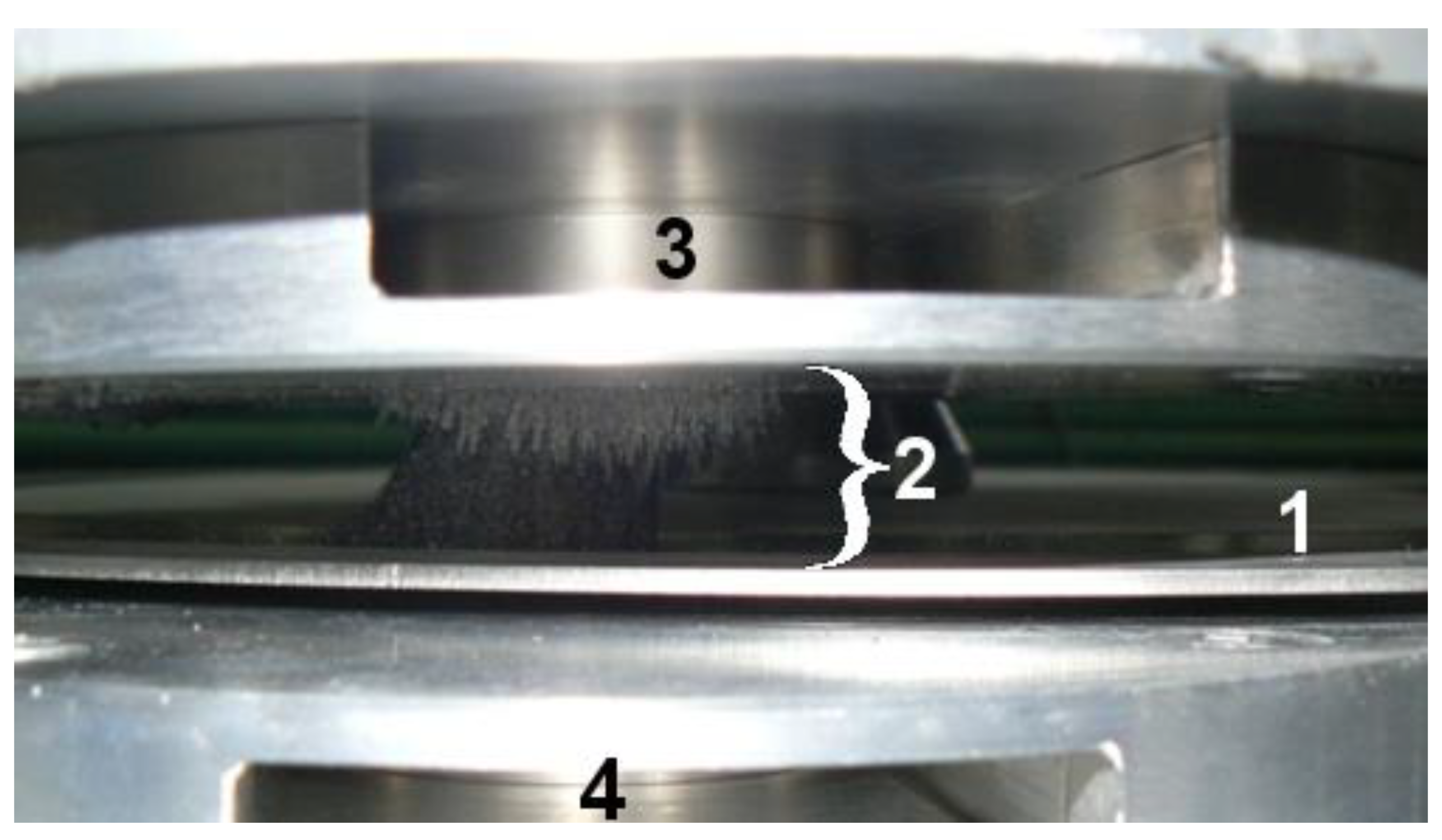
- Concentration of abrasive grains K [%]. This was determined on the basis of the machining gap dimensions at a limited volume of field interaction between the upper and lower magnets, and then converted to abrasive grain mass for each sample. For each gap width, the volume of the machining zone was calculated by taking a cylinder with a diameter of 50 mm (diameter of the magnets). For a known container volume, the mass of abrasive grains was measured to obtain the volume density. The mass of abrasive grains that should be delivered to the machining zone in each test was calculated.
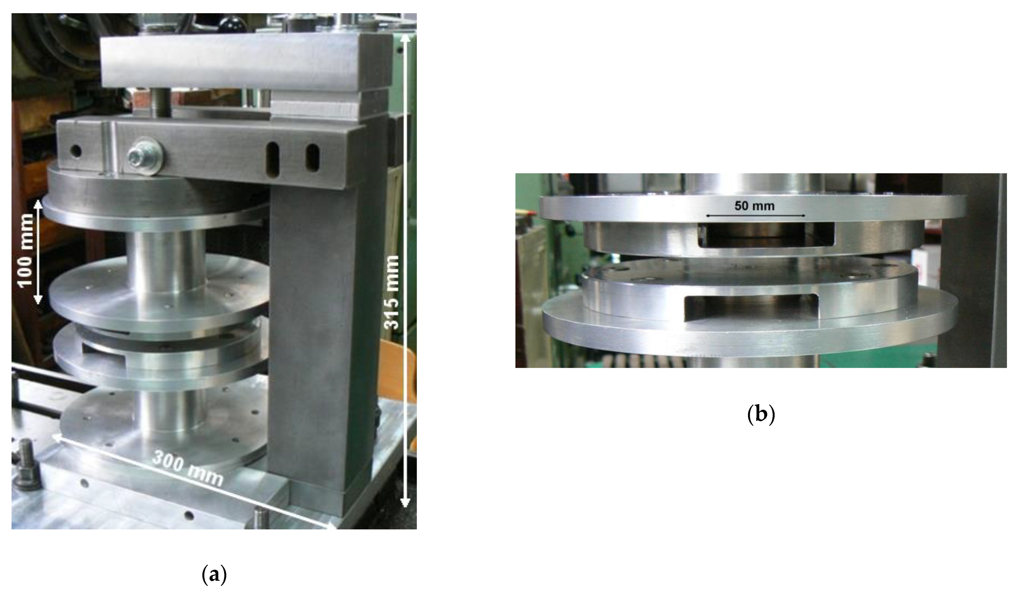
- Machining gap width S [mm]. This is the distance between the stacks of upper and lower magnets. It was calculated as the width of the machining gap after taking into account the separators holding the magnets and separating the abrasive grains from them.
- Machining time T [min]. This was selected on the basis of literature data.
- rpm n = 85 rpm (average machining speed V = 80 m/min, for diameter from axis to center of machining area d = 300 mm),
- abrasive grains Fe–TiC 315/200 (~30 µm),
- AISI 304L stainless steel (Table 3), dimensions of round plate equal ɸ370 mm × 2 mm.
3. Results and Discussion
3.1. Simulation
3.2. Measurement
3.3. Design of Experiment
4. Conclusions
- Within the assumed range of machining parameters, the surface layer of AISI 304L stainless steel improved, so that precision increased and better surface quality of manufacturing elements was achieved.
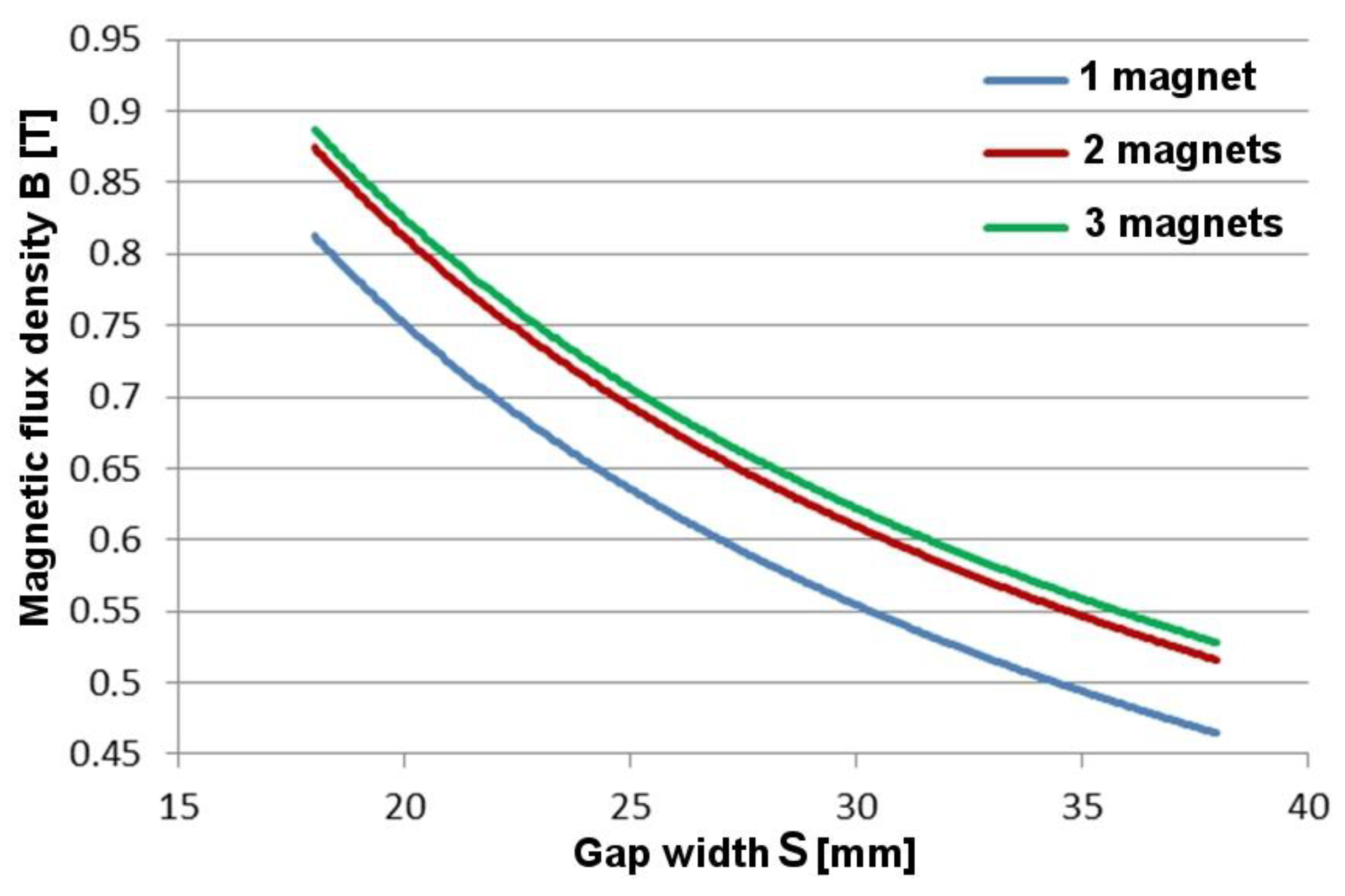
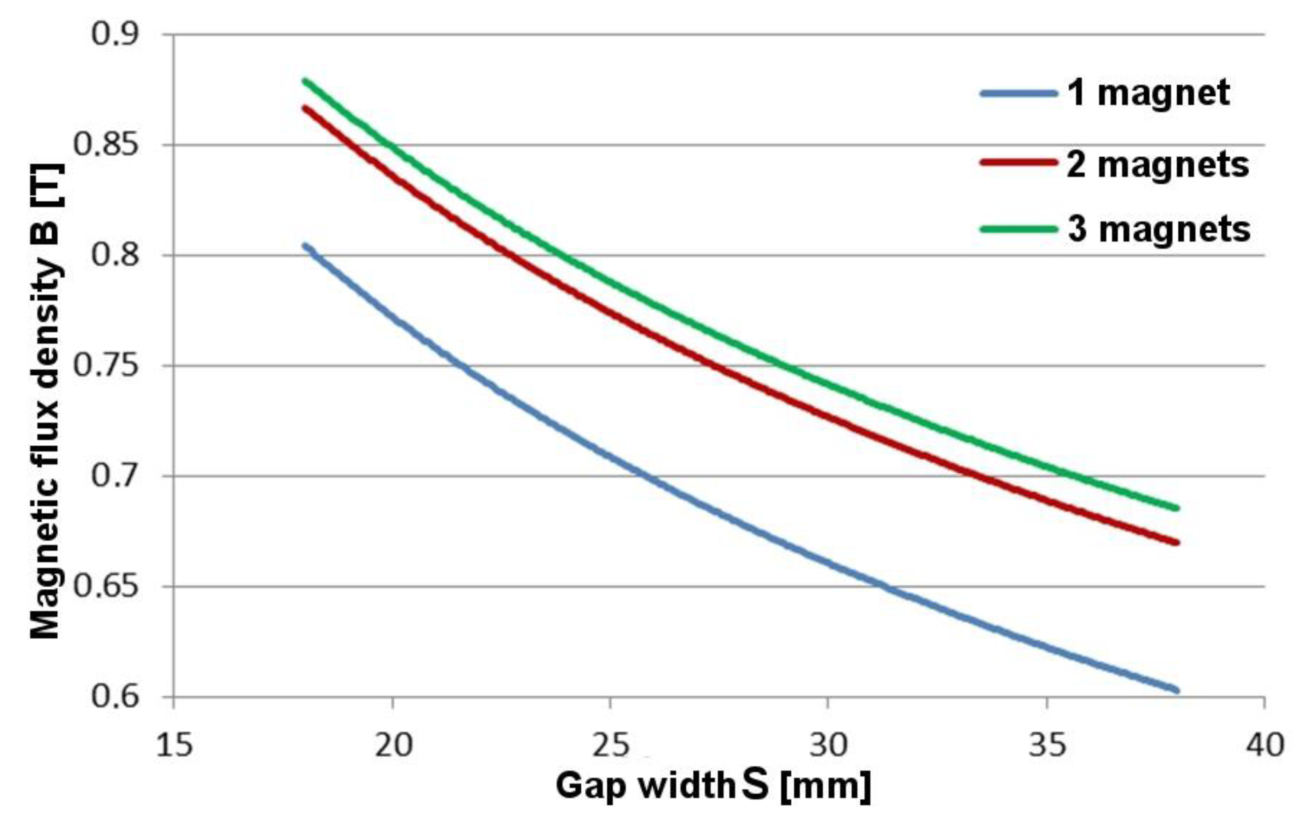
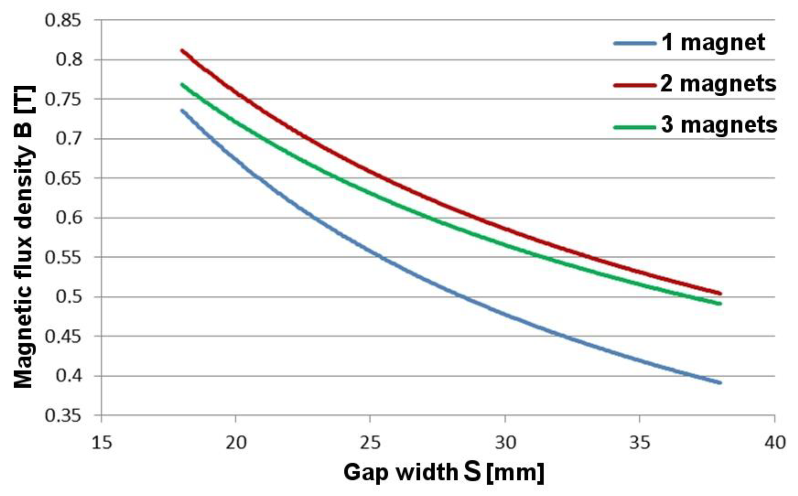
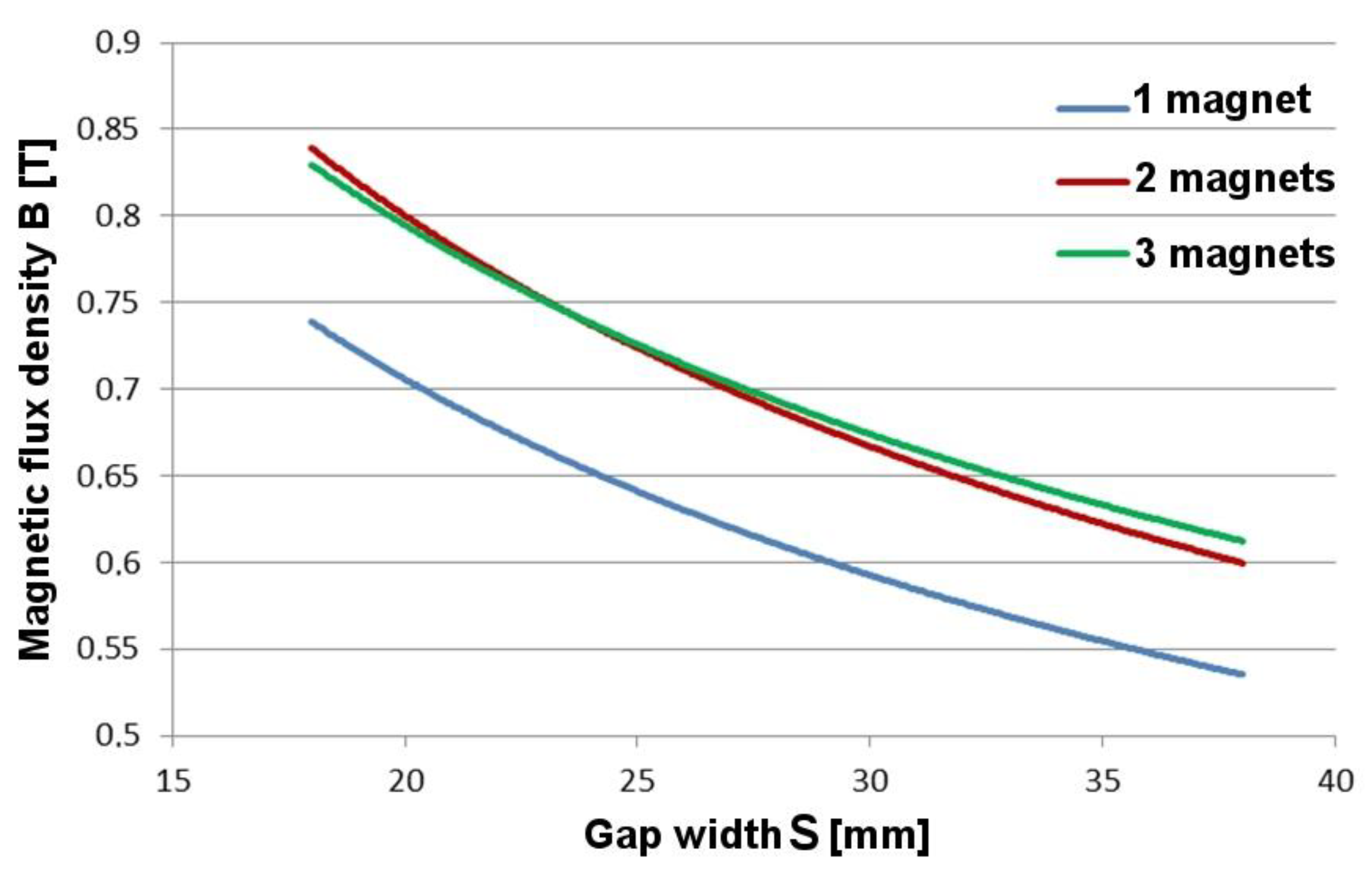
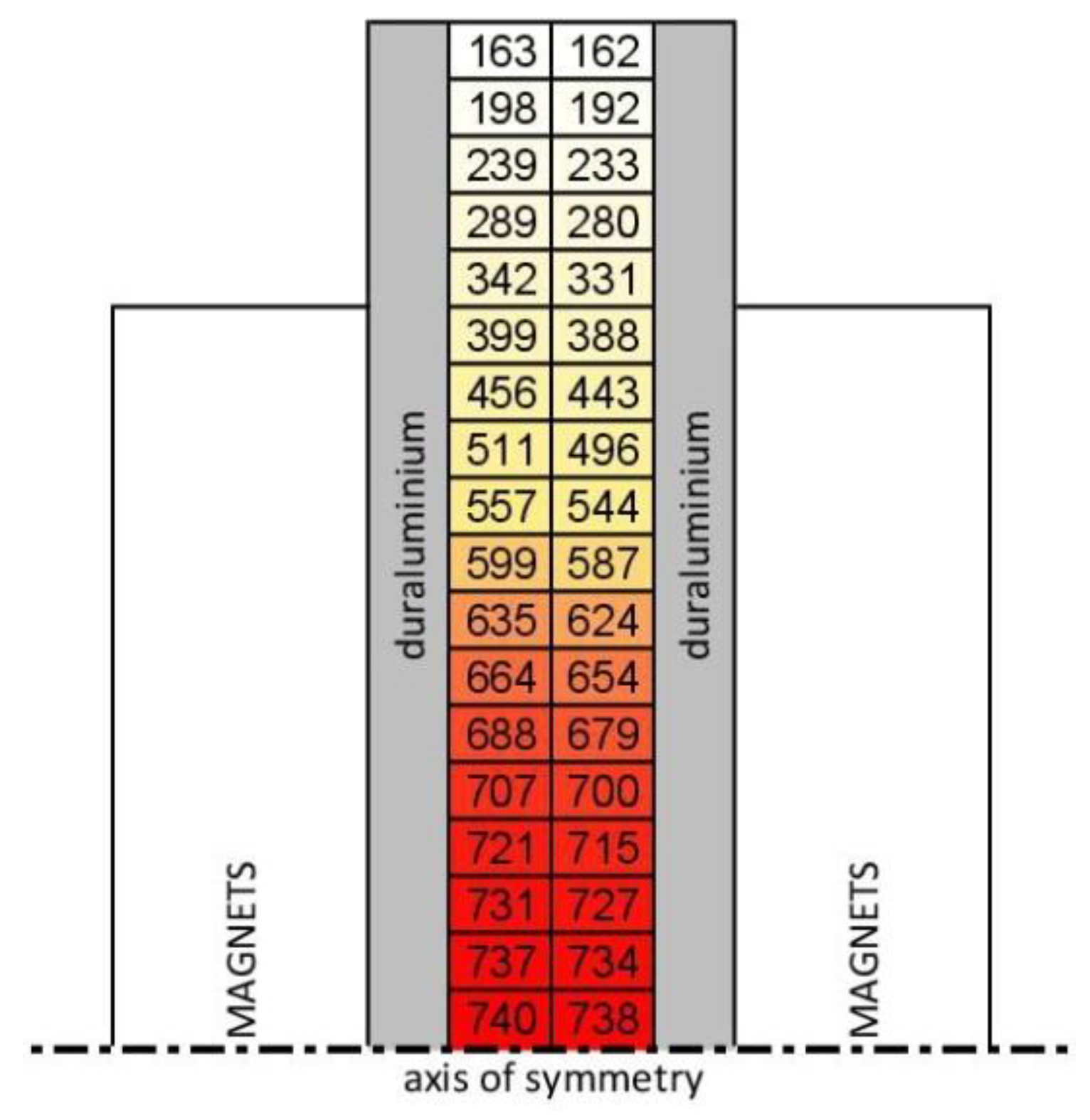
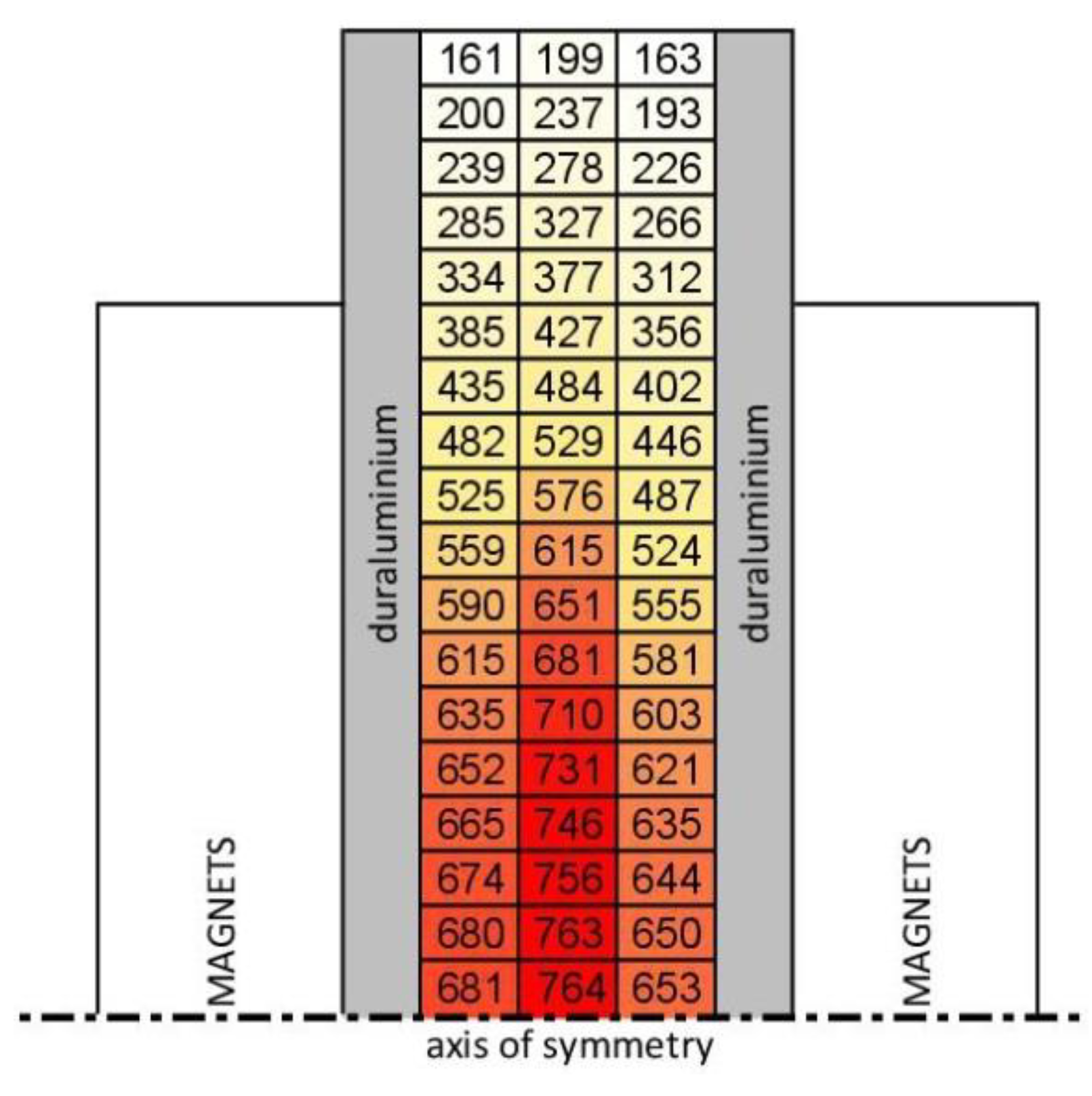
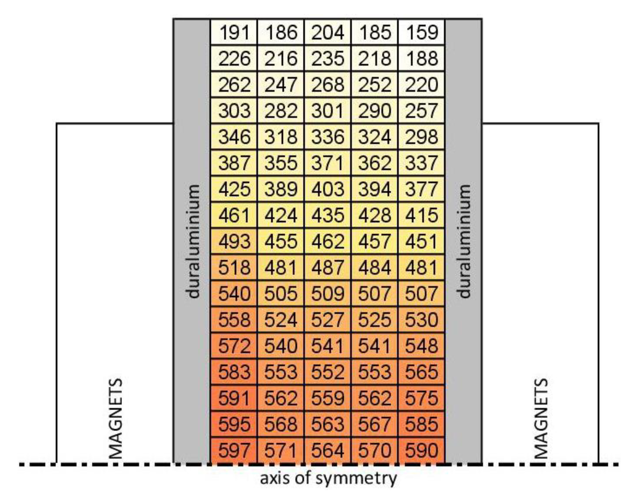
- Based on the conducted numerical simulation we were able to determine the approximate relation between the number of magnets in the stack and the maximum magnetic flux density in the machining gap. The greater the number of magnets, the greater the value of magnetic flux density was, although this relation was not linear, which is shown by the distance between consecutive curves (Figure 7 and Figure 8).
- It should be noted that the difference in the values of magnetic flux density in the center of the machining gap and on the separator’s surface was not constant. It grew with the number of magnets and the width of the machining gap.
- The proposed magnetic abrasive machining station is characterized by the ability to produce significant magnetic flux density values in the range of 0.4–0.85 T, i.e., in the upper limits of the magnetic flux density values found in the literature [30]. Such high magnetic flux density values translate into a relatively high force acting on the abrasive grain. This may partially increase the material removal rate.
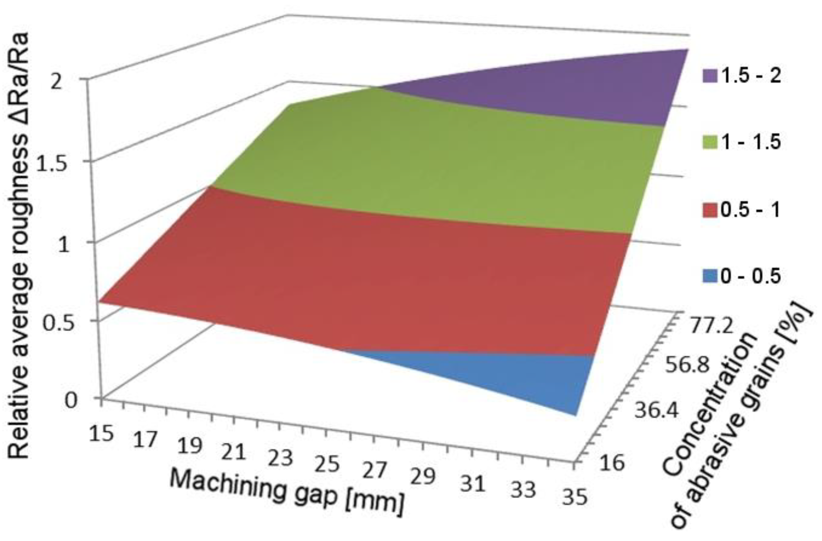
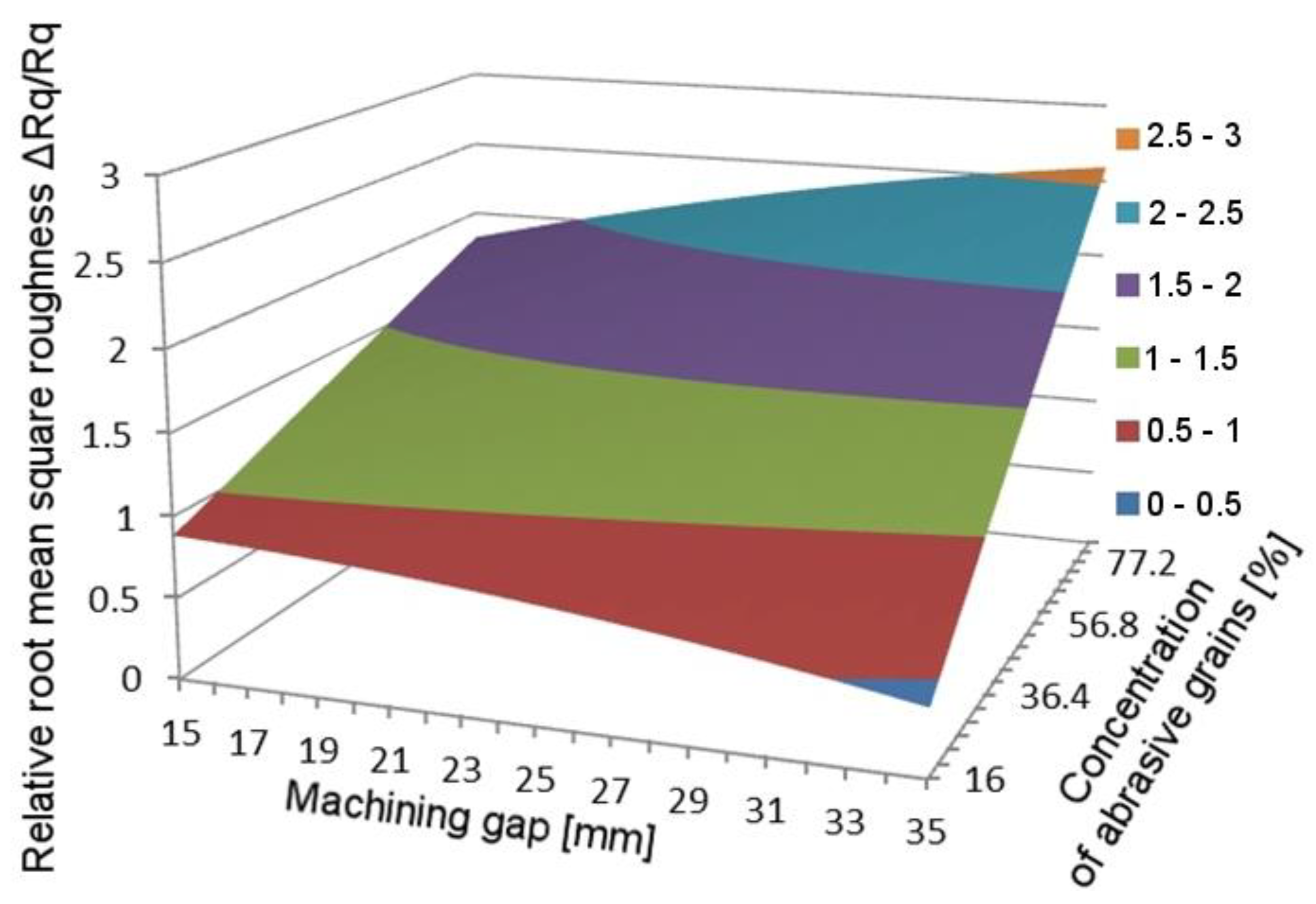
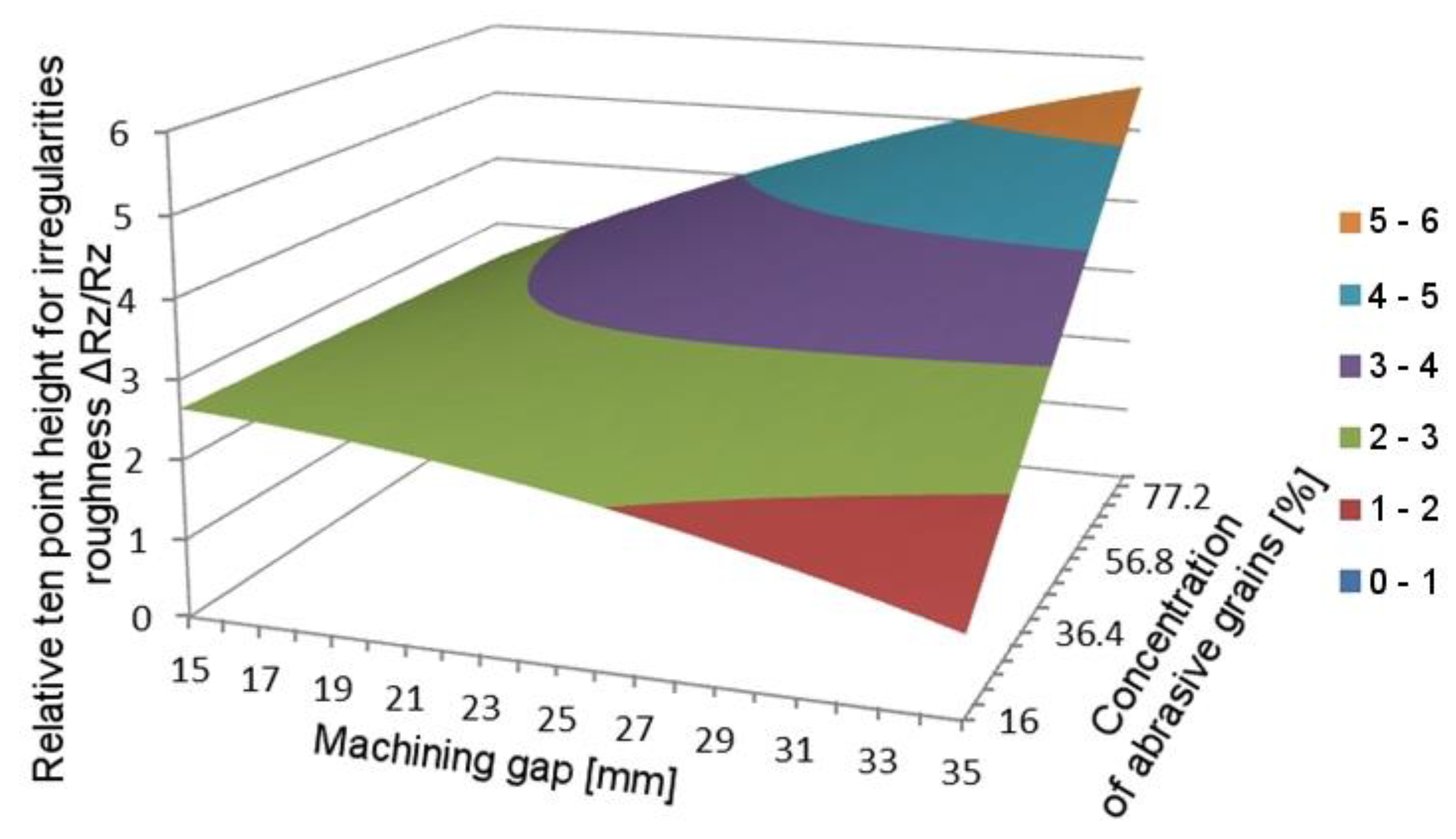
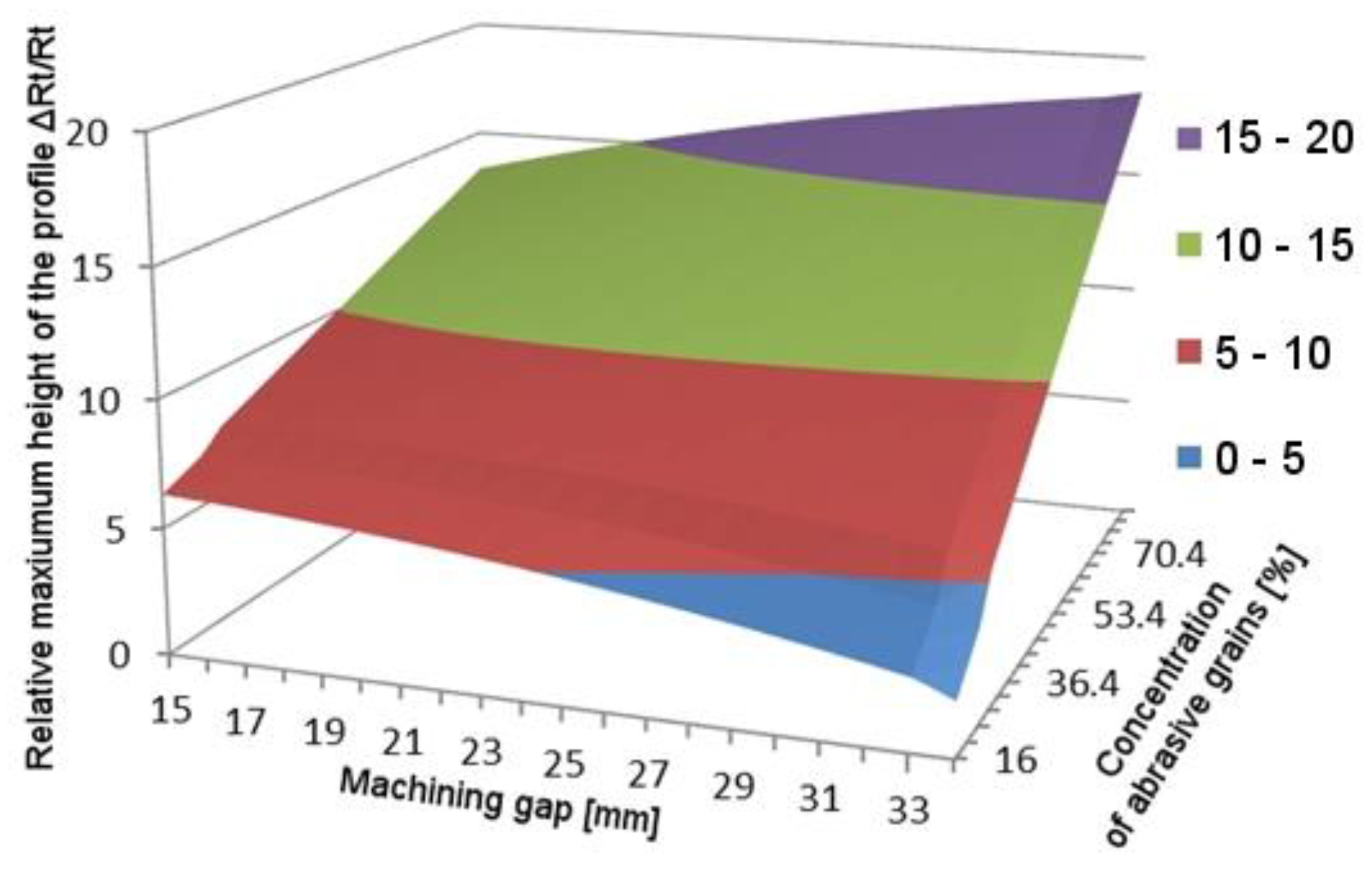
- The maximum relative change in ΔRa/Ra, ΔRq/Rq, ΔRz/Rz, and ΔRt/Rt roughness is directly proportional to the number of abrasive grains in the working gap (Figure 22). At the same time, this does not mean that the greater the quantity of abrasive material, the greater the number of grains involved in the microcutting process.
- The relative change of roughness parameters for the smallest concentration of abrasive grains (K = 16%) is negligible. The number of abrasive grains is not sufficient for an efficient machining process. The reason for this is the accumulation of a significant amount of abrasive grains at the top head. These grains do not take part in the machining process. With a concentration of more than 70%, the frictional force between the workpiece and the grains may increase significantly as a result of abrasive grain jamming, which may clamp the workpiece.
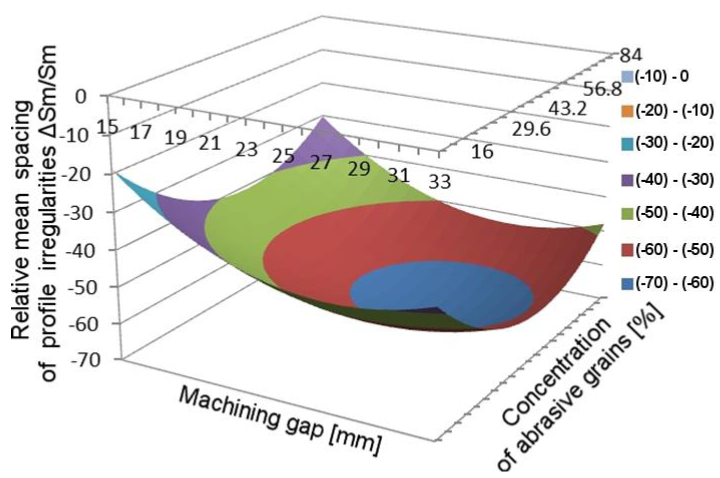
- The effect of the machining gap width is increasingly significant if the concentration of abrasive grains increases.
- For small machining gap widths, an increase in the concentration of abrasive grains has little effect on lowering the Ra, Rq, Rz, and Rt roughness parameters. However, when we widen the machining gap, the concentration’s impact on these parameters increases. This may result from the perpendicular movement of abrasive grains relative to the width of the machining gap (Figure 30).
- The experiment results indicate the smooth character of the processing [31]. A very significant improvement in the roughness value was observed for certain ranges of parameters. The greatest influence can be observed for the mean spacing of profile irregularities Sm. This is a premise to undertake further experiments that would take into account a larger number of horizontal roughness parameters (e.g., mean summit curvature, RMS surface slope).
Author Contributions
Funding
Institutional Review Board Statement
Informed Consent Statement
Data Availability Statement
Conflicts of Interest
Nomenclature
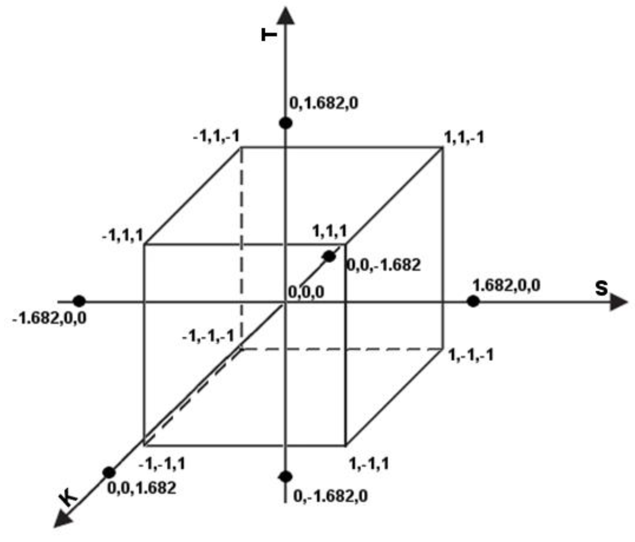
| a | the star radius at design of experiment for 20 tests (a = 1.682) |
| B | magnetic induction or magnetic flux density [T] |
| BHmax | energy density [kJ/m3] |
| Br | residual magnetism [T] |
| d | diameter of the sample distance from center of the round plate to the center of permanent magnets [mm] |
| h | machining gap width, the distance between the upper and lower separators (h = S - 8) [mm] |
| jHc | coercion [kA/m] |
| K | concentration of abrasive grains in meaning filling the cylindrical space between magnets [%] |
| m | mass of abrasive grains [g] |
| n | round per minute (85 rpm) |
| R | correlation coefficient |
| Ra | roughness average [μm] |
| Rq | root mean square average of the profile heights over the evaluation length [μm] |
| Rt | maximum height of the profile [μm] |
| Rz | average maximum height of the profile [μm] |
| S | machining gap width, the distance between the stacks upper and lower of magnets [mm] |
| SEM | scanning electron microscope |
| Sa | arithmetical mean height [μm] |
| Sm | mean spacing of profile irregularities [μm] |
| Sq | root mean square height [μm] |
| St | peak-peak height (ASME B46.1) [μm] |
| Sz | peak-peak height (ISO 4287/1) [μm] |
| T | machining time [min] |
| V | average machining speed |
| ɸ0 | magnetic flux [Wb] |
References
- Fernandez-Zelaia, P.; Melkote, S.N. Process–structure–property relationships in bimodal machined microstructures using robust structure descriptors. J. Mater. Process. Technol. 2019, 273, 116251. [Google Scholar] [CrossRef]
- Singh, R.K.; Gangwar, S.; Singh, D.K. Experimental investigation on temperature-affected magnetic abrasive finishing of Aluminum 6060. Mater. Manuf. Process. 2019, 34, 1274–1285. [Google Scholar] [CrossRef]
- Kumar, S.; Singh, A.K. Magnetorheological nanofinishing of BK7 glass for lens manufacturing. Mater. Manuf. Process. 2018, 33, 1188–1196. [Google Scholar] [CrossRef]
- Barman, A.; Das, M. Simulation and experimental investigation of finishing forces in magnetic field assisted finishing process. Mater. Manuf. Process. 2018, 33, 1223–1232. [Google Scholar] [CrossRef]
- Kim, J.S.; Nam, S.S.; Heng, L.; Kim, B.S.; Mun, S.D. Effect of environmentally friendly oil on Ni-Ti stent wire using ultraprecision magnetic abrasive finishing. Metals 2020, 10, 1309. [Google Scholar] [CrossRef]
- Zhang, J.; Hu, J.; Wang, H.; Kumar, A.S.; Chaudhari, A. A novel magnetically driven polishing technique for internal surface finishing. Precis. Eng. 2018, 54, 222–232. [Google Scholar] [CrossRef]
- Singh, M.; Singh, A.K. Magnetorheological finishing of micro-punches for enhanced performance of micro-extrusion process. Mater. Manuf. Process. 2019, 34, 1646–1657. [Google Scholar] [CrossRef]
- Singh, M.; Singh, A.K. Improved magnetorheological finishing process with rectangular core tip for external cylindrical surfaces. Mater. Manuf. Process. 2019, 34, 1049–1061. [Google Scholar] [CrossRef]
- Grover, V.; Singh, A.K. Improved magnetorheological honing process for nanofinishing of variable cylindrical internal surfaces. Mater. Manuf. Process. 2018, 33, 1177–1187. [Google Scholar] [CrossRef]
- Kariganaur, K.A.; Kumar, H.; Arun, M. Effect of magnetic permeability, shearing length, and shear gap on magnetic flux density of the magnetorheological damper through finite element analysis. Mater. Today Proc. 2020, S2214785320343261. [Google Scholar] [CrossRef]
- Mosavat, M.; Rahimi, A. Numerical-Experimental study on polishing of silicon wafer using magnetic abrasive finishing process. Wear 2019, 424–425, 143–150. [Google Scholar] [CrossRef]
- Kum, C.W.; Sato, T.; Guo, J.; Liu, K.; Butler, D. A novel media properties-based material removal rate model for magnetic field-assisted finishing. Int. J. Mech. Sci. 2018, 141, 189–197. [Google Scholar] [CrossRef]
- Gao, Y.; Zhao, Y.; Zhang, G.; Yin, F.; Zhang, H. Modeling of material removal in magnetic abrasive finishing process with spherical magnetic abrasive powder. Int. J. Mech. Sci. 2020, 177, 105601. [Google Scholar] [CrossRef]
- Song, J.; Shinmura, T.; Mun, S.D.; Sun, M. Micro-Machining characteristics in high-speed magnetic abrasive finishing for fine ceramic bar. Metals 2020, 10, 464. [Google Scholar] [CrossRef]
- Iqbal, F.; Jha, S. Experimental investigations into transient roughness reduction in ball-end magneto-rheological finishing process. Mater. Manuf. Process. 2019, 34, 224–231. [Google Scholar] [CrossRef]
- Wu, P.-Y.; Yamaguchi, H. Material removal mechanism of additively manufactured components finished using magnetic abrasive finishing. Procedia Manuf. 2018, 26, 394–402. [Google Scholar] [CrossRef]
- Kumar, H.; Singh, S.; Srivastava, A. Parametric investigations into internal surface modification of brass tubes with alternating magnetic field. Procedia Manuf. 2016, 5, 1234–1248. [Google Scholar] [CrossRef]
- Singh, R.K.; Singh, D.K.; Gangwar, S. Advances in magnetic abrasive finishing for futuristic requirements–A review. Mater. Today Proc. 2018, 5, 20455–20463. [Google Scholar] [CrossRef]
- Tumański, S. Handbook of Magnetic Measurements; Series in Sensors; Taylor & Fracis: Boca Raton, FL, USA, 2011; ISBN 978-1-4398-2951-6. [Google Scholar]
- Angus, H.T. Cast Iron; Elsevier Science: Burlington, ON, Canada, 1976; ISBN 978-1-4831-0195-8. [Google Scholar]
- Manyala, R. A Guide to Small-Scale Energy Harvesting Techniques; IntechOpen: London, UK, 2020; ISBN 978-1-78923-910-2. [Google Scholar]
- Permanent Magnets. 2015. Available online: www.magnesy.pl (accessed on 5 September 2018).
- Antony, J. Design of Experiments for Engineers and Scientists, 2nd ed.; Elsevier insights; Elsevier: London, UK, 2014; ISBN 978-0-08-099417-8. [Google Scholar]
- Srivastava, A.; Kumar, H.; Singh, S. Investigations into internal surface finishing of titanium (grade 2) pipe with extended magnetic tool. Procedia Manuf. 2018, 26, 181–189. [Google Scholar] [CrossRef]
- Davis, J.R. (Ed.) Stainless Steels. In ASM Specialty Handbook; ASM International: Materials Park, OH, USA, 1994; ISBN 978-0-87170-503-7. [Google Scholar]
- Li, W.; Li, X.; Yang, S.; Li, W. A newly developed media for magnetic abrasive finishing process: Material removal behavior and finishing performance. J. Mater. Process. Technol. 2018, 260, 20–29. [Google Scholar] [CrossRef]
- Gupta, B.; Jain, A.; Purohit, R.; Rana, R.S.; Gupta, B. Effects of process parameters on the surface finish of flat surfaces in magnetic assist abrasive finishing process. Mater. Today Proc. 2018, 5, 17725–17729. [Google Scholar] [CrossRef]
- Singh, L.; Khangura, S.S.; Mishra, P.S. Performance of abrasives used in magnetically assisted finishing: A state of the art review. IJAT 2010, 3, 215. [Google Scholar] [CrossRef]
- Gao, Y.; Zhao, Y.; Zhang, G.; Zhang, G.; Yin, F. Polishing of paramagnetic materials using atomized magnetic abrasive powder. Mater. Manuf. Process. 2019, 34, 604–611. [Google Scholar] [CrossRef]
- Mulik, R.S.; Pandey, P.M. Magnetic abrasive finishing of hardened AISI 52100 steel. Int. J. Adv. Manuf. Technol. 2011, 55, 501–515. [Google Scholar] [CrossRef]
- Yin, C.; Wang, R.; Kim, J.; Lee, S.; Mun, S. Ultra-high-speed magnetic abrasive surface micro-machining of AISI 304 cylindrical bar. Metals 2019, 9, 489. [Google Scholar] [CrossRef]


| Material Designation and Properties | Chemical Composition [%] | ||
|---|---|---|---|
| Grade AISI | 60-40-18 | C | 3.5–3.8 |
| Grade DIN | GGG-40 | Mn | 0.15–0.35 |
| Grade BS | 420/112 | Si | 2.2–2.8 |
| Tensile strength Rm min [MPa] | 400 | P | 0.02–0.06 |
| Proof stress R0.2 min [MPa] | 250 | S | 0.01–0.025 |
| Relative elongation A5 [%] | 12 | Mg | 0.03–0.065 |
| Permanent Magnet (N42). | |
|---|---|
| Dimensions [mm] | ɸ 50 × 20 |
| Magnetic flux ɸ0 [Wb] | 0.107 |
| Coercion jHc [kA/m] | 1091 |
| Residual magnetism Br [T] | 1.28 |
| Energy density (BHmax) [kJ/m3] | 318–342 |
| Maximum temperature [°C] | 80 |
| Standard/Parameters | Mark/Value | Chemical Composition[%] | |
|---|---|---|---|
| Grade AISI | 304L | C | 0.03 |
| Grade DIN | 1.4307 | Mn | 2 |
| Grade BS | 304S11 | Si | ≤1 |
| Tensile strength Rm min [MPa] | 620 | P | 0.045 |
| Proof stress R0.2 min [MPa] | 310 | S | 0.03 |
| Relative elongation A5 [%] | 45 | Cr | 18–20 |
| Ni | 10.5 | ||
| N | 0.1 | ||
| Star arm a | −1.682 | −1 | 0 | 1 | 1.682 |
| S [mm] | 15 | 18 | 23 | 28 | 35 |
| T [min] | 7 | 10 | 15 | 20 | 27 |
| K [%] | 16 | 30 | 50 | 70 | 84 |
| Nr. | K [%] | S [mm] | T [min] | m [g] | h [mm] |
|---|---|---|---|---|---|
| 9 | 50 | 15 | 15 | 4.55 | 7 |
| 1 | 30 | 18 | 10 | 6.82 | 10 |
| 3 | 30 | 18 | 20 | 6.82 | 10 |
| 13 | 16 | 23 | 15 | 7.28 | 15 |
| 5 | 70 | 18 | 10 | 15.92 | 10 |
| 7 | 70 | 18 | 20 | 15.92 | 10 |
| 2 | 30 | 28 | 10 | 20.47 | 20 |
| 4 | 30 | 28 | 20 | 20.47 | 20 |
| 11 | 50 | 23 | 7 | 22.75 | 15 |
| 12 | 50 | 23 | 27 | 22.75 | 15 |
| 15 | 50 | 23 | 15 | 22.75 | 15 |
| 16 | 50 | 23 | 15 | 22.75 | 15 |
| 17 | 50 | 23 | 15 | 22.75 | 15 |
| 18 | 50 | 23 | 15 | 22.75 | 15 |
| 19 | 50 | 23 | 15 | 22.75 | 15 |
| 20 | 50 | 23 | 15 | 22.75 | 15 |
| 14 | 84 | 23 | 15 | 38.21 | 15 |
| 6 | 70 | 28 | 10 | 47.77 | 20 |
| 8 | 70 | 28 | 20 | 47.77 | 20 |
| 10 | 50 | 35 | 15 | 50.04 | 27 |
| Gap S [mm] | Maximal Value B [T] |
|---|---|
| 23 | 0.74 |
| 28 | 0.76 |
| 33 | 0.59 |
| 38 | 0.57 |
| 43 | 0.45 |
| Roughness Parameters | Before Machining | After Machining |
|---|---|---|
| Sa [μm] | 2.53 | 0.85 |
| Sq [μm] | 3.08 | 1.08 |
| St [μm] | 25.2 | 12.6 |
| Sz [μm] | 23.7 | 11.5 |
| Roughness Parameters | Before Machining | After Machining |
|---|---|---|
| Ra [μm] | 1.52 | 0.47 |
| Rq [μm] | 1.73 | 0.56 |
| Rz [μm] | 6.48 | 2.37 |
| Rt [μm] | 9.68 | 8.68 |
| Sm [μm] | 49.9 | 79.4 |
Publisher’s Note: MDPI stays neutral with regard to jurisdictional claims in published maps and institutional affiliations. |
© 2021 by the authors. Licensee MDPI, Basel, Switzerland. This article is an open access article distributed under the terms and conditions of the Creative Commons Attribution (CC BY) license (http://creativecommons.org/licenses/by/4.0/).
Share and Cite
Marczak, M.; Zawora, J. Finite Element Analysis of the Magnetic Field Distribution in a Magnetic Abrasive Finishing Station and its Impact on the Effects of Finishing Stainless Steel AISI 304L. Metals 2021, 11, 194. https://doi.org/10.3390/met11020194
Marczak M, Zawora J. Finite Element Analysis of the Magnetic Field Distribution in a Magnetic Abrasive Finishing Station and its Impact on the Effects of Finishing Stainless Steel AISI 304L. Metals. 2021; 11(2):194. https://doi.org/10.3390/met11020194
Chicago/Turabian StyleMarczak, Michał, and Józef Zawora. 2021. "Finite Element Analysis of the Magnetic Field Distribution in a Magnetic Abrasive Finishing Station and its Impact on the Effects of Finishing Stainless Steel AISI 304L" Metals 11, no. 2: 194. https://doi.org/10.3390/met11020194
APA StyleMarczak, M., & Zawora, J. (2021). Finite Element Analysis of the Magnetic Field Distribution in a Magnetic Abrasive Finishing Station and its Impact on the Effects of Finishing Stainless Steel AISI 304L. Metals, 11(2), 194. https://doi.org/10.3390/met11020194