Abstract
Experimental assays and mathematical models, through population balance models (PBM), were used to characterize the particle aggregation of mining tailings flocculated in seawater. Three systems were considered for preparation of the slurries: i) Seawater at natural pH (pH 7.4), ii) seawater at pH 11, and iii) treated seawater at pH 11. The treated seawater had a reduced magnesium content in order to avoid the formation of solid complexes, which damage the concentration operations. For this, the pH of seawater was raised with lime before being used in the process—generating solid precipitates of magnesium that were removed by vacuum filtration. The mean size of the aggregates were represented by the mean chord length obtained with the Focused beam reflectance measurement (FBRM) technique, and their descriptions, obtained by the PBM, showed an aggregation and a breakage kernel had evolved. The fractal dimension and permeability were included in the model in order to improve the representation of the irregular structure of the aggregates. Then, five parameters were optimized: Three for the aggregation kernel and two for the breakage kernel. The results show that raising the pH from 8 to 11 was severely detrimental to the flocculation performance. Nevertheless, for pH 11, the aggregates slightly exceeded 100 µm, causing undesirable behaviour during the thickening operations. Interestingly, magnesium removal provided a suitable environment to perform the tailings flocculation at alkaline pH, making aggregates with sizes that exceeded 300 µm. Only the fractal dimension changed between pH 8 and treated seawater at pH 11—as reflected in the permeability outcomes. The PBM fitted well with the experimental data, and the parameters showed that the aggregation kernel was dominant at all-polymer dosages. The descriptive capacity of the model might have been utilized as a support in practical decisions regarding the best-operating requirements in the flocculation of copper tailings and water clarification.
1. Introduction
High-salinity resources, such as seawater, are being used in the mining industry in countries such as Australia, Chile, and Indonesia. At first, saltwater was proceeded by desalination plants, primarily through reverse osmosis (RO). Unfortunately, RO has created the new challenge of concentrated brine by-product, which is released into the environment; the effluent has a high temperature and a high demand for electricity, which involves fossil fuel consumption. Therefore, the direct use of seawater without ion removal is an attractive strategy that has recently been implemented in many mining industries. In this matter, engineers and researchers are constantly studying certain operational complexities. Some of these studies focus on the corrosion and incrustation of pipelines, the precipitate complexes, and the buffer effect of seawater. An example is the concentration of Cu/Mo ores, where a high level of pyrite is found, which drastically hinders the efficiency of the flotation process. The depression of pyrite in freshwater lime is used to bring the operation to an alkaline pH condition (>10.5), where the hydrophilic ferric hydroxide is formed. Nevertheless, this condition cannot function in seawater because the formation of solid Ca/Mg complexes strongly decreases the recovery of molybdenite [1,2] and chalcopyrite [3,4]. There is a debate as to the proper explanation of these findings in the sulphide flotation [5,6,7,8], but the recovery of water for the sustainability of the mining industry is more important. This is necessary due to the high cost of transporting seawater to mining sites; in Chile, the mining site can be as much as 4000 m above sea level. An essential process in the recovery of water is the thickening stage, where efficiency is linked to the flocculation of the suspended particles, which promotes solid–liquid separation. The flocculants are long water-soluble polyelectrolytes that can bridge multiple particles and form aggregates that are sedimentary because of the effects of gravity. The conventional flocculant used in copper mining is hydrolyzed polyacrylamide (HPAM) with a high molecular weight, which gives high settling rates, low densities, and proper rheological properties of concentrated underflows at relatively low doses and low cost [9,10]. Several efforts have been made in the study of HPAM behaviour in the solution [11,12] and high-saline conditions [13,14,15]. These studies provide enough proof that bridging flocculation may benefit from a saline medium because ions can act as a bridge between the anionic solid particles and anionic flocculants, commonly known as ion binding. However, the concentrated salt can reduce the size of the reagents by an excess of charge neutralization. These studies were performed on chloride salt solutions; seawater has a complex mix of ions, where Ca and Mg are present, and as we know, at high-alkaline conditions, they precipitate into a hydroxide complex. Recent studies show that kaolinite can adsorb several heavy metal ions [16,17] and also hydroxide complexes [18]; therefore, these precipitates have a strong interaction with solid particles and possibly, the flocculants. These results provide evidence that precipitates can affect the flocculation mechanism and negatively affect the thickener performance. However, this might be avoided by removing magnesium ions prior to incorporating the seawater in the operations.
A good strategy to analyze flocculation performance is by monitoring the aggregate size distribution over time by the focused beam reflectance measurement (FBRM), which has the advantage of being employed directly to the slurry without sampling or the need for dilution [19,20,21,22]. In flocculated systems, a maximum floc size is achieved after a short time following flocculant addition; it then follows a decay that emerges from the fragmentation of the aggregates and polymer depletion. Using the FBRM has provided an excellent method to analyze flocculation parameters such as the maximum aggregation size or fragmentation rate [23,24,25,26]. In this context, many researchers have described the kinetics of aggregate growth and fragmentation over time by population balance models (PBM) [27,28,29,30], which have practical applications in a wide variety of systems [31,32,33,34,35]. The PBM is based on the work by Smoluchowski [27,36], which describes how aggregates evolve over time. Such evolution depends on the mechanisms of the aggregation and the rupture of the equations. To update the PBM to flocculation, it is necessary to improve the physical description of the aggregates by (1) updating the collision efficiency to a time-dependent flocculant depletion [30,35], and (2) to use the fractal dimension as an indicator of the irregular structure of the aggregates [27,36,37,38,39,40]. Recently, we have proven that, for these flocculated systems, it is possible to use a constant fractal dimension when the shear rate is below 200 s−1.
In this work, we use PBM to describe the flocculation kinetics of tailing particles using treated seawater with the magnesium removed in order to improve the water recovery and the performance of the thickening stages. Then, we analyze the implications of precipitates being present for phenomena such as collision frequency, collision efficiency, fragmentation rate, and floc permeability. The outcomes of this work are of particular interest to mining industries that use seawater in concentration stages, and the implementation of this plan might allow for sustainable results without the need to totally remove seawater salts by reverse osmosis.
2. Methodology
2.1. Materials
The seawater (SW) was obtained from the San Jorge Bay in Antofagasta (Chile); to eliminate bacterial activity, the SW was filtered at 1 μm using a UV filter system. This water had a conductivity of 50.4 mS/cm, while its ionic composition was the following: 10.9 g/L Na+, 1.38 g/L Mg2+, 0.4 g/L Ca2+, 0.39 K+, 19.6 Cl−, and 0.15 g/L HCO3− [41].
Kaolin was acquired from Ward’s Science, and a quantitative X-ray diffraction (XRD) analysis showed that it contained 84 wt% kaolinite (Al2Si2O5(OH)4) and 16 wt% halloysite (Al2Si2O5(OH)4·2H2O) (Figure 1). A D5000 X-ray diffractometer (Siemens S.A., Lac Condes, Chile) was used and the data were processed with Total Pattern Analysis Software (TOPAS) (Siemens S.A., Lac Condes, Chile). Quartz was acquired from a local Chilean store, where the SiO2 content detected by quantitative XRD was over 99 wt% (see Figure 2). Both quartz and kaolin had a density of 2.6 g/t. A Microtrac S3500 laser diffraction particle size analyzer (Verder Scientific, Newtown, PA, USA) was used. The analysis showed that 10% of the particles were smaller than d10 = 1.8 and 3.8 µm in the kaolin and quartz samples, respectively.
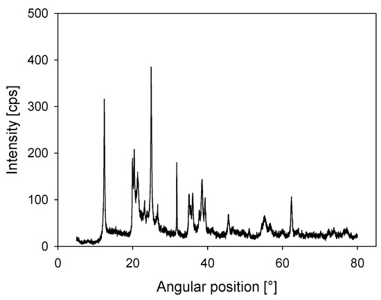
Figure 1.
X-ray diffraction (XRD) for kaolin powder.
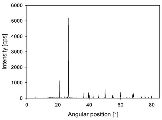
Figure 2.
X-ray diffraction (XRD) for quartz powder.
SNF 704, provided by SNF Chile S.A., was used as an anionic flocculant. The molecular weight was higher than 18 × 106. An initial stock solution was prepared at a concentration of 1 g/L. Then, it was mixed with a low RPM for 24 h before use, stored in a refrigerator, and discarded after two weeks in order to avoid the potential ageing effect. An aliquot of this stock flocculant solution was diluted at 0.1 g/L once a day for use in testing, with unused portions, then discarded. The flocculant dosages were determined in terms of grams of polymer per ton of dry solids (g/ton). The reagents used to modify the pH were lime and sodium hydroxide and were of analytical grade (greater than 98%).
2.2. Magnesium Removal
The removal of magnesium was carried out by increasing the pH of the seawater with 0.06 M of lime in order to form hydroxide magnesium as a white precipitate. In parallel, bicarbonate was reacted with Mg to form magnesium carbonate [41]. After 30 min of intense mixing, the seawater was vacuum filtered, obtaining seawater with an ionic concentration of 10.9 g/L Na+, 0.01 g/L Mg2+, 2.35 g/L Ca2+, 0.39 K+, 19.6 Cl−, and 0.05 g/L HCO3.
2.3. Flocculant-Suspension
A suspension of 270 g was prepared at 8 wt%, with known masses of the solid phases to give mixtures containing 80 wt% quartz and 20 wt% kaolin. The suspension was vigorously mixed for 30 min using a 30 mm-diameter turbine type stirrer within a 100 mm-diameter vessel with a 1 L capacity. All the experiments were made by placing the stirrer 20 mm above the bottom of the vessel. Subsequently, the mixing rate was controlled at 250 rpm, and the volume of the solution (seawater and polymer) was added in a proportion fixed by the required polymer dosage.
2.4. Batch Settling Tests
These tests were conducted, after 30 s of flocculant-suspension mixing, by gently pouring the slurry into closed, 300 cm3 cylinders (35 mm internal diameter), and then slowly inverting the cylinder two times by hand (the whole cylinder rotation process took, in all cases, about 4 s). After 10 min of settling, the supernatant fluid was rescued and stirred in order to homogenize the suspended solids. Then, a 50 mL aliquot was used for turbidity measurements in a HANNA HI98713 turbidimeter (Hanna Instruments, Santiago, Chile), which performed ten readings in 20 s, delivering the average at the end of that period.
2.5. Characterization of Aggregates
The FBRM technique was used to record the chord length distribution of the aggregates. The probe was submerged vertically in the reaction vessel, 10 mm over the stirrer and 20 mm off-axis. The FBRM probe featured a laser that was focused through the sapphire window and scanned a circular path at a tangential velocity of 2 m/s. The backscattered light was then received when the laser beam intersected the path of the particle or aggregate. A chord length was determined from the duration of any unusual increase in the backscattered light intensity and laser velocity.
3. Modeling
The PBM equations used in this work are derived from several works [42,43,44] that discretize the aggregate size into the number i of the bins. Every bin is based on the classical geometric distribution for the aggregate volume (Vi+1) = 2Vi). The PBM equation is given by:
where is the number concentration of the aggregates in bin , whereas is the number concentration of primary particles in bin 1. Every term on the right of the equation represents a physical process:
- The first and second terms describe the aggregate formation of size i from smaller aggregates.
- The third and fourth terms describe the aggregation death of size i to higher aggregates.
- The fifth term represents the breakage formation of size i from the rupture of a greater aggregate.
- The sixth term represents the breakage death of size i by creating smaller aggregates.
The superscript max1 is the maximum number of intervals used to represent the complete aggregate size spectrum; max2 corresponds to the largest interval from which the aggregates in the current range are produced.
3.1. Aggregation Kernel
The Q variable is the aggregation kernel, an expression that contains the collision frequency (β) and capture efficiency (α):
Collision Frequency β
It has been shown that fluid flow can penetrate through particle aggregates [45]. This means that the actual collision frequency is considerably lower than that predicted from rectilinear flow models. To add the permeability effects to the collision frequency, we use the parameter called “fluid collection efficiency” η. This measures the ratio between the flow passing through the aggregate and the flow approaching it. Veerapaeni and Wiesner [46] proposed a function to calculate the collision frequency, which includes the permeability and fractal dimension effects:
where, and are the diameters of the aggregates sizes of and , respectively, G is the shear rate, and η is derived from the Brinkman’ extension to Darcy’s laws as a function of a dimensionless permeability (ξ) [47]:
where is defined as and Ki is the permeability; we use the expression from the work by Li and Logan [47]:
The porosity ϕ is related to the fractal dimension () using the expression by Vainshtein et al. [48]:
where C is a packing coefficient (generally assumed to be 0.65) and the primary particle diameter. and are related by the expression proposed by Mandelbrot [49]:
Collision Efficiency α
There are several expressions for collision efficiency, which depend on the type of aggregate and the additives. In this case, we use an expression to represent the effect of high-weight polymers; this is the polymer depletion and it rearranges on the adsorbed surface of the particles. This has been implemented in a recent work by Vajihinejad and Soares [35], which showed an exponential decay between two fitted parameters:
where is the maximum collision efficiency, is the minimum collision efficiency (at steady-state conditions), and is the collision efficiency decay constant ().
3.2. Breakage Kernel
In regards to Equation (1), the S term is the breakage rate and Γ is the distribution breakage, which represents the breakage kernel. The S term is difficult to predict since there is no theory and is usually fitted to the size distribution data. In this case, we use a power-law function of the aggregate mass, as proposed by Pandya and Spielman [50]:
where and are the fitted parameters.
To simplify the distribution breakage, we use a binary distribution, where an aggregate breaks into two pieces of equal mass. That is:
3.3. Shear Rate
The shear rate required by the aggregation and breakage kernels is calculated from:
where is the average energy dissipation rate:
where is the impeller power number (0.6 in our case for a plane disk with gentle agitation [51]), is the rotation speed, and are, respectively, the diameter of the impeller and the working volume of the vessel. The density of the suspension is calculated from:
where is the solid mass fraction of the solution, and are, respectively, the solid and water density. Finally, the viscosity of the solution is measured.
3.4. Solution
To resolve the PBM in Equation (1), we use a solver based on the numerical differentiation formula for stiff ODEs (ode23s) in MATLAB. The optimization was performed with the MATLAB function fminsearch, which uses the Nelder–Mead direct search to find the minimum in an unconstrained multivariable function. The objective function () used to optimize the parameters is given by:
where is the experimental diameter of the particles, and is the model diameter obtained by:
Two criteria validate the model’s fit and predictions: One is the coefficient of determination (), which measures the closeness of the model values to the experimental values. That is:
and the other is the quality of the fit:
std stands for the standard error calculated from:
where is the number of data values and is the number of parameters to be fitted. A of 90% or higher means that the proposed model can predict the flocculation kinetics. Finally, conservation of the total volume of particles is verified after every integration in order to ensure that the simulations maintain the particle population.
4. Results
4.1. Input Parameters and Distribution
Three cases were studied: Seawater at pH 8 (SW pH 8), seawater at pH 11 (SW pH 11), and treated seawater at pH 11 (T-SW pH 11), with Mg removed. Solving the PBM equations requires a set of input parameters (Table 1). With these parameters, the shear rate can be calculated from Equations (11)–(13) and the rest are used for the PBM equation definitions. A particle number concentration is needed for each size class and for each unit of volume of suspension . For that, a number distribution is obtained from experimental results through , where is the volume fraction of particles with diameter , obtained from Equation (7), is the solid volume fraction and is the volume of the primary particles following the geometric progression . To obtain the , a volume distribution is needed. Figure 3A shows an experimental volume fraction distribution provided from the FRPM probe for three case studies before the flocculant is added; in this case, all distributions are similar. To calculate the fractal dimension from the settings test, we follow the procedure by Heath et al. [20]. The fractal dimension results are shown in Figure 3B. The fractal dimension is higher when the flocculant dose increases. At pH 11, the fractal dimension decreases abruptly because the solid magnesium precipitates would produce open structures. Nevertheless, the treated seawater overcomes this phenomenon, giving similar structures to those of the pH 8 system.

Table 1.
Input parameters and conditions.
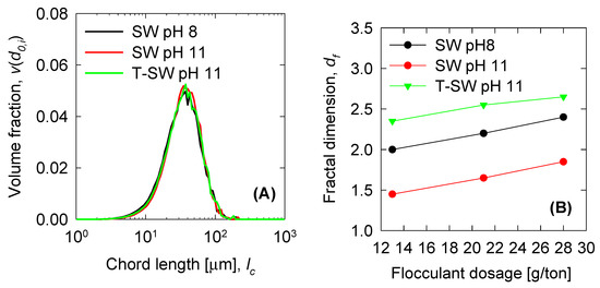
Figure 3.
(A) Normalized initial volume distribution of particles of synthetic tailings in seawater at a mixing rate of 150 rpm. (B) Fractal dimension from the settling experiments.
4.2. Flocculation Kinetics and Modeling
The results of the experimental data are plotted in Figure 4 for the three cases studied in this work. We see that the flocculant doses increase the size of the aggregates, which is similar to other work, as shown in Reference [35]. For SW pH 8, the aggregate increases to a maximum value of 300 µm for the flocculant dose of 28 g/ton. Smaller values are obtained when the flocculant dose decreases. If we increase the pH to 11 (SW pH 11), we see results similar to those in Figure 4B, where the aggregate falls to a smaller value of ~100 µm for all the flocculant doses in this work. This behaviour is primarily related to the formation of hydroxide complexes that hinder aggregate formation. Later, we see the results of Mg removal from the seawater before being added to the slurry at pH 11 (T-SW pH 11). In this case, we have a higher maximum aggregation than when Mg is present as a hydroxide. From this, we can clearly see that Mg hydroxide presence hinders the aggregation process drastically. Then, the PBM modeling in the figures are included in the results as continuous lines. As we see from Table 2, there is a good agreement for the cases where the mean aggregate diameter is higher, but there are limitations associated with the model for the examples that are small in size.
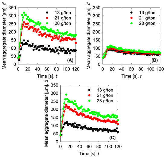
Figure 4.
Flocculation kinetics of synthetic tailings in seawater as a function of flocculant doses (mixing rate 150 rpm). Solid circles correspond to experimental data and solid lines to the best fit with the population balance model (PBM). (A) Seawater (SW) pH 8. (B) SW pH 11. (C) Treated (T)-SW pH 11.
Table 2.
Quantitative results of GoF and R2 when the PBM model is used.
4.3. Optimized Parameters
The model fitted five parameters: The maximum and minimum collision efficiency (), the collision efficiency decay constant (), and two breakage rate kernel parameters ( and ). The first three parameters are related to the aggregation kernel and are shown in Figure 5. The show a steady increase when the flocculant dose increases. This reflects the activity of the flocculant to aggregate more significant quantities of solids at higher doses. Interestingly, the has small values compared to the , and all remain below 0.02, meaning that, at steady state (where becomes significant), the breakage kernel must also be small. , as we found in previous results, must follow the inverse tendency of the because the higher the aggregates, the greater the probability of flocculant depletion. In this case, the fitted parameters also show that behaviour. Finally, if we compare the three trials, we see that the parameters of the SW at pH 8 are similar of the T-SW at pH 11, which implies that the removal of the Mg could keep the aggregation performance similar to that of pH 8. Finally, the two parameters for the breakage kernel are plotted in Figure 6. As discussed above, if the s1 is small, the is also small. This trend must be followed in order to satisfy steady-state conditions in the aggregation process. The s2 parameters show values between 1 and 2, but as the s1 parameter is small, its contribution is neglected from the global behavior. From this, we see that high dosage increments contribute to the aggregate kernel rather than the breakage kernel.
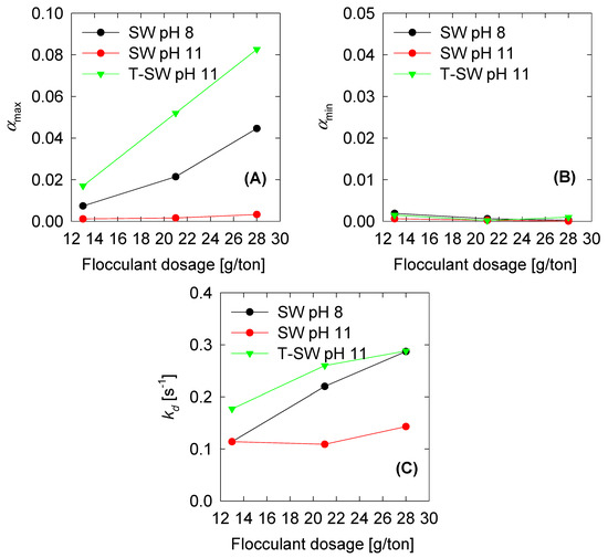
Figure 5.
Optimum aggregation parameters vs. shear rate for constant and variable fractal dimension: (A) Maximum and (B) minimum collision efficiency and (C) collision efficiency decay constant .
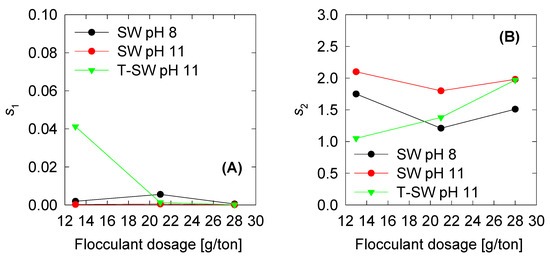
Figure 6.
Optimum breakage parameters vs. shear rate for constant and variable fractal dimension: (A) S1 and (B) collision efficiency decay constant .
4.4. Aggregation, Breakage, and Permeability Modeling
Once we have the optimized parameters, we can compute the physical parameters: Collision efficiency, collision frequency, breakage rate, and permeability with the mean aggregate size from the results in Figure 4. Collision frequencies are shown in Figure 7. We see that high doses of flocculant increase the collision frequency. This can be accounted for by the polymer concentration, which has an extended configuration that increases the likelihood of collisions. For SW pH 11, the small aggregates generated by the appearance of magnesium complexes lead to a low value in the collision frequency. This does not present significant changes with varied flocculant doses. Calculations for collision efficiency are presented in Figure 8 and follow the same trend as the collision frequency, where SW pH 11 has no significant values. In this case, only below 20 s is the parameter relevant to the kinetics, and drops to zero values after 20 s. Breakage rates are shown in Figure 9, which shows that, at SW pH 8, we see that low doses generate higher values because less flocculant cannot maintain the aggregates. We see similar behaviour in SW pH 11 and T-SW pH 11; this is accounted for because of the fractal dimensions. For SW at pH 11, the fractal dimension is low, and the diameter increase coincided with an increased breakage rate. For T-SW at pH 11, the fractal dimension is high, decreasing the aggregate diameter and decreasing the breakage rate, even if the aggregates are big. Finally, permeability results were plotted in Figure 10; we can see that very porous aggregates are found for SW pH 8 and a dose of 21 g/ton. This can be accounted for by the fractal dimension and the large mean size of the aggregates. For SW at pH 11, we see that permeability is lower even if the fractal dimension is small, because the size of the aggregate is small in these cases. Interestingly, the permeability value for T-SW pH 11 is low, as compared to other cases, even if the aggregate sizes are similar to those in SW pH 8. This is because the fractal dimension is high and creates dense aggregates that have little permeability.
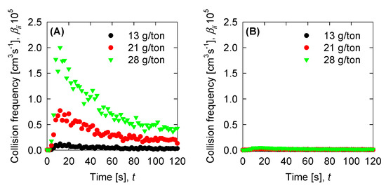
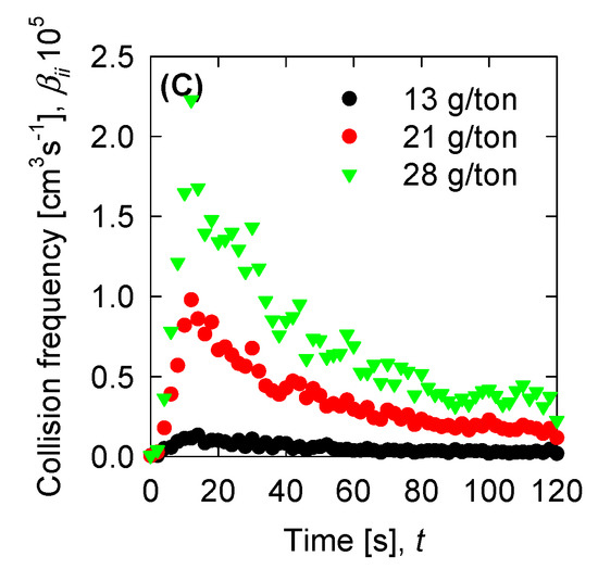
Figure 7.
Collision frequency for the experimental data for (A) SW pH 8, (B) SW pH 11, and (C) T-SW pH 11.
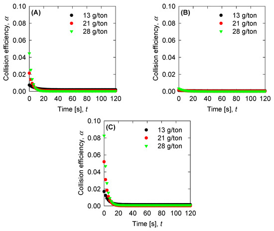
Figure 8.
Collision efficiency for the experimental data for (A) SW pH 8, (B) SW pH 11, and (C) T-SW pH 11.
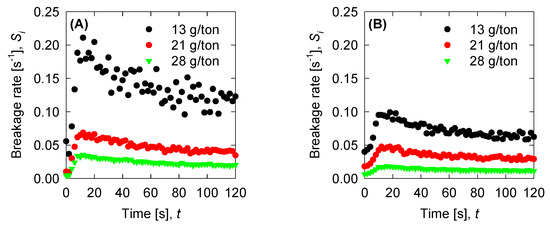
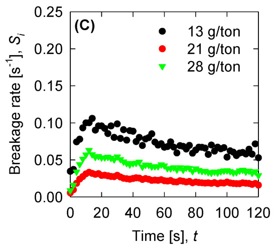
Figure 9.
Breakage rate for the experimental data for (A) SW pH 8, (B) SW pH 11, and (C) T-SW pH 11.
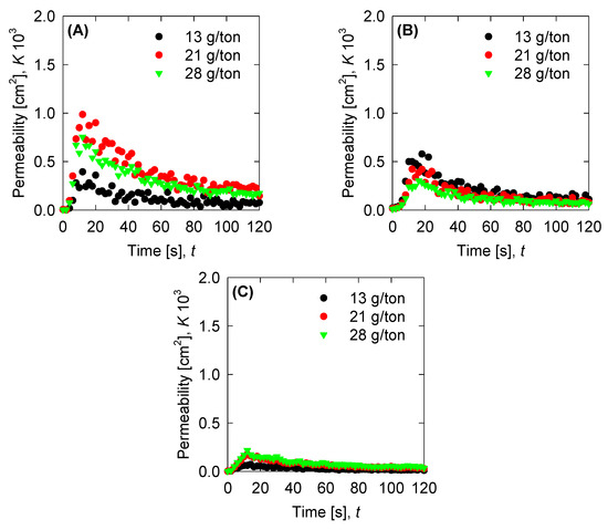
Figure 10.
Permeability for the experimental data for (A) SW pH 8, (B) SW pH 11, and (C) T-SW pH 11.
5. Conclusions
Experiments and modeling, through a population balance model (PBM), are used to characterize the particle aggregation of flocculated tailings on untreated and treated seawater (SW) at different flocculant doses. It was found that the Mg hydroxide complex presence could hinder the aggregate kinetics drastically over time; this generates small aggregates between 50–100 microns at pH 11. If the Mg is removed before the flocculation takes place, we can obtain larger aggregates, from 100–200 microns, at the same pH. The results of T-SW pH 11 are in good agreement with the SW pH 8 achievements, which may imply that pH is no longer a restrictive parameter for the aggregation process. The modeling of the aggregation was done with PBM, where fitted parameters can represent the flocculation aggregation kinetics. In this case, the effect of flocculant dose can neglect the impact of the breakage kernel, and the aggregation kernel dominates the flocculation. Additionally, it is found that, without Mg ions, the pH has little effect on both the flocculation kinetics and PBM fitted parameters. Only the fractal dimension shows us the main difference between SW pH 8 and T-SW pH 11, where it is reflected in its permeability. As we can see, experiments and modeling show us that the Mg removal is the main component that hinders particle aggregation, and without its presence, the process can operate similarly at neutral pH and high pH.
Author Contributions
All of the authors contributed to the analysis of the results and writing the paper. All authors have read and agreed to the published version of the manuscript
Funding
This research was funded by ANID Fondecyt 11171036, ANID ACM 170005, and Centro CRHIAM Project ANID/Fondap/15130015.
Acknowledgments
Gonzalo Quezada and Ricardo I. Jeldres thank the Centro CRHIAM Project ANID/Fondap/15130015. Ricardo I. Jeldres thanks ANID Fondecyt 11171036 and ANID ACM 170005. Pedro Robles thanks the Pontificia Universidad Católica de Valparaíso for the support provided.
Conflicts of Interest
The authors declare no conflict of interest.
References
- Qiu, Z.; Liu, G.; Liu, Q.; Zhong, H. Understanding the roles of high salinity in inhibiting the molybdenite flotation. Colloids Surfaces A Physicochem. Eng. Asp. 2016. [Google Scholar] [CrossRef]
- Li, W.; Li, Y.; Wei, Z.; Xiao, Q.; Song, S. Fundamental studies of SHMP in reducing negative effects of divalent ions on molybdenite flotation. Minerals 2018, 8, 404. [Google Scholar] [CrossRef]
- Li, Y.; Li, W.; Xiao, Q.; He, N.; Ren, Z.; Lartey, C.; Gerson, A. The influence of common monovalent and divalent chlorides on chalcopyrite flotation. Minerals 2017, 7, 111. [Google Scholar] [CrossRef]
- Uribe, L.; Gutierrez, L.; Laskowski, J.S.; Castro, S. Role of calcium and magnesium cations in the interactions between kaolinite and chalcopyrite in seawater. Physicochem. Probl. Miner. Process. 2017, 53, 737–749. [Google Scholar] [CrossRef]
- Ramos, O.; Castro, S.; Laskowski, J.S. Copper–molybdenum ores flotation in sea water: Floatability and frothability. Miner. Eng. 2013, 53, 108–112. [Google Scholar] [CrossRef]
- Hirajima, T.; Suyantara, G.P.W.; Ichikawa, O.; Elmahdy, A.M.; Miki, H.; Sasaki, K. Effect of Mg2+ and Ca2+ as divalent seawater cations on the floatability of molybdenite and chalcopyrite. Miner. Eng. 2016, 96–97, 83–93. [Google Scholar] [CrossRef]
- Jeldres, R.I.; Arancibia-Bravo, M.P.; Reyes, A.; Aguirre, C.E.; Cortes, L.; Cisternas, L.A. The impact of seawater with calcium and magnesium removal for the flotation of copper-molybdenum sulphide ores. Miner. Eng. 2017, 109, 10–13. [Google Scholar] [CrossRef]
- Suyantara, G.P.W.; Hirajima, T.; Miki, H.; Sasaki, K. Floatability of molybdenite and chalcopyrite in artificial seawater. Miner. Eng. 2018, 115, 117–130. [Google Scholar] [CrossRef]
- Lee, L.T.; Rahbari, R.; Lecourtier, J.; Chauveteau, G. Adsorption of polyacrylamides on the different faces of kaolinites. J. Colloid Interface Sci. 1991, 147, 351–357. [Google Scholar] [CrossRef]
- Nasser, M.S.; James, A.E. Effect of polyacrylamide polymers on floc size and rheological behaviour of kaolinite suspensions. Colloids Surfaces A Physicochem. Eng. Asp. 2007, 301, 311–322. [Google Scholar] [CrossRef]
- Zhang, L.; Zheng, L.; Pu, J.; Pu, C.; Cui, S. Influence of hydrolyzed polyacrylamide (hpam) molecular weight on the cross-linking reaction of the HPAM/Cr3+ System and transportation of the HPAM/Cr3+ system in microfractures. Energy Fuels 2016. [Google Scholar] [CrossRef]
- Abdel-Azeim, S.; Kanj, M.Y. Dynamics, Aggregation, and Interfacial Properties of the Partially Hydrolyzed Polyacrylamide Polymer for Enhanced Oil Recovery Applications: Insights from Molecular Dynamics Simulations. Energy Fuels 2018. [Google Scholar] [CrossRef]
- Quezada, G.R.; Jeldres, R.I.; Fawell, P.D.; Toledo, P.G. Use of molecular dynamics to study the conformation of an anionic polyelectrolyte in saline medium and its adsorption on a quartz surface. Miner. Eng. 2018, 129, 102–105. [Google Scholar] [CrossRef]
- Quezada, G.R.; Saavedra, J.H.; Rozas, R.E.; Toledo, P.G. Molecular dynamics simulations of the conformation and diffusion of partially hydrolyzed polyacrylamide in highly saline solutions. Chem. Eng. Sci. 2019. [Google Scholar] [CrossRef]
- Jeldres, M.; Piceros, E.C.; Toro, N.; Torres, D.; Robles, P.; Leiva, W.H.; Jeldres, R.I. Copper tailing flocculation in seawater: Relating the yield stress with fractal aggregates at varied mixing conditions. Metals 2019, 9, 1295. [Google Scholar] [CrossRef]
- Jiang, M.Q.; Jin, X.Y.; Lu, X.Q.; Chen, Z.L. Adsorption of Pb(II), Cd(II), Ni(II) and Cu(II) onto natural kaolinite clay. Desalination 2010. [Google Scholar] [CrossRef]
- Bhattacharyya, K.G.; Gupta, S.S. Adsorption of a few heavy metals on natural and modified kaolinite and montmorillonite: A review. Adv. Colloid Interface Sci. 2008, 140, 114–131. [Google Scholar] [CrossRef]
- Diamond, S.; Kinter, E.B. Adsorption of calcium hydroxide by montmorillonite and kaolinite. J. Colloid Interface Sci. 1966. [Google Scholar] [CrossRef]
- Biggs, C.A.; Lant, P.A. Activated sludge flocculation: On-line determination of floc size and the effect of shear. Water Res. 2000. [Google Scholar] [CrossRef]
- Heath, A.R.; Bahri, P.A.; Fawell, P.D.; Farrow, J.B. Polymer flocculation of calcite: Relating the aggregate size to the settling rate. AIChE J. 2006, 52, 1987–1994. [Google Scholar] [CrossRef]
- Gregory, J. Monitoring particle aggregation processes. Adv. Colloid Interface Sci. 2009, 147–148, 109–123. [Google Scholar] [CrossRef] [PubMed]
- Meng, Z.; Hashmi, S.M.; Elimelech, M. Aggregation rate and fractal dimension of fullerene nanoparticles via simultaneous multiangle static and dynamic light scattering measurement. J. Colloid Interface Sci. 2013, 392, 27–33. [Google Scholar] [CrossRef] [PubMed]
- Heath, A.R.; Bahri, P.A.; Fawell, P.D.; Farrow, J.B. Polymer flocculation of calcite: Experimental results from turbulent pipe flow. AIChE J. 2006, 52, 1284–1293. [Google Scholar] [CrossRef]
- Owen, A.T.; Fawell, P.D.; Swift, J.D.; Labbett, D.M.; Benn, F.A.; Farrow, J.B. Using turbulent pipe flow to study the factors affecting polymer-bridging flocculation of mineral systems. Int. J. Miner. Process. 2008, 87, 90–99. [Google Scholar] [CrossRef]
- Bubakova, P.; Pivokonsky, M.; Filip, P. Effect of shear rate on aggregate size and structure in the process of aggregation and at steady state. Powder Technol. 2013, 235, 540–549. [Google Scholar] [CrossRef]
- Benn, F.A.; Fawell, P.D.; Halewood, J.; Austin, P.J.; Costine, A.D.; Jones, W.G.; Francis, N.S.; Druett, D.C.; Lester, D. Sedimentation and consolidation of different density aggregates formed by polymer-bridging flocculation. Chem. Eng. Sci. 2018, 184, 111–125. [Google Scholar] [CrossRef]
- Thomas, D.N.; Judd, S.J.; Fawcett, N. Flocculation modelling: a review. Water Res. 1999, 33, 1579–1592. [Google Scholar] [CrossRef]
- Heath, A.R.; Bahri, P.A.; Fawell, P.D.; Farrow, J.B. Polymer flocculation of calcite: Population balance model. AIChE J. 2006, 52, 1641–1653. [Google Scholar] [CrossRef]
- Jeldres, R.I.; Fawell, P.D.; Florio, B.J. Population balance modelling to describe the particle aggregation process: A review. Powder Technol. 2018, 326, 190–207. [Google Scholar] [CrossRef]
- Quezada, G.R.; Ramos, J.; Jeldres, R.I.; Robles, P.; Toledo, P.G. Analysis of the flocculation process of fine tailings particles in saltwater through a population balance model. Sep. Purif. Technol. 2019, 237, 116319. [Google Scholar] [CrossRef]
- Runkana, V.; Somasundaran, P.; Kapur, P.C. A population balance model for flocculation of colloidal suspensions by polymer bridging. Chem. Eng. Sci. 2006, 61, 182–191. [Google Scholar] [CrossRef]
- Costa, C.B.B.; Maciel, M.R.W.; Filho, R.M. Considerations on the crystallization modeling: Population balance solution. Comput. Chem. Eng. 2007, 31, 206–218. [Google Scholar] [CrossRef]
- Datta, A.; Rajamani, R.K. A direct approach of modeling batch grinding in ball mills using population balance principles and impact energy distribution. Int. J. Miner. Process. 2002, 64, 181–200. [Google Scholar] [CrossRef]
- Kiparissides, C.; Alexopoulos, A.; Roussos, A.; Dompazis, G.; Kotoulas, C. Population balance modeling of particulate polymerization processes. Ind. Eng. Chem. Res. 2004, 43, 7290–7302. [Google Scholar] [CrossRef]
- Vajihinejad, V.; Soares, J.B.P. Monitoring polymer flocculation in oil sands tailings: A population balance model approach. Chem. Eng. J. 2018, 346, 447–457. [Google Scholar] [CrossRef]
- Jeldres, R.I.; Concha, F.; Toledo, P.G. Population balance modelling of particle flocculation with attention to aggregate restructuring and permeability. Adv. Colloid Interface Sci. 2015, 224, 62–71. [Google Scholar] [CrossRef]
- Ahmad, A.L.; Chong, M.F.; Bhatia, S. Population Balance Model (PBM) for flocculation process: Simulation and experimental studies of palm oil mill effluent (POME) pretreatment. Chem. Eng. J. 2008, 140, 86–100. [Google Scholar] [CrossRef]
- Flesch, J.C.; Spicer, P.T.; Pratsinis, S.E. Laminar and turbulent shear-induced flocculation of fractal aggregates. AIChE J. 1999, 45, 1114–1124. [Google Scholar] [CrossRef]
- Selomulya, C.; Bushell, G.; Amal, R.; Waite, T.D. Understanding the role of restructuring in flocculation: The application of a population balance model. Chem. Eng. Sci. 2003, 58, 327–338. [Google Scholar] [CrossRef]
- Antunes, E.; Garcia, F.A.P.; Ferreira, P.; Blanco, A.; Negro, C.; Rasteiro, M.G. Modelling PCC flocculation by bridging mechanism using population balances: Effect of polymer characteristics on flocculation. Chem. Eng. Sci. 2010, 65, 3798–3807. [Google Scholar] [CrossRef]
- Jeldres, M.; Piceros, E.; Robles, P.A.; Toro, N.; Jeldres, R.I. Viscoelasticity of quartz and kaolin slurries in seawater: Importance of magnesium precipitates. Metals 2019, 9, 1120. [Google Scholar] [CrossRef]
- Spicer, P.T.; Pratsinis, S.E. Shear-induced flocculation: The evolution of floc structure and the shape of the size distribution at steady state. Water Res. 1996, 30, 1049–1056. [Google Scholar] [CrossRef]
- Hounslow, M.J.; Ryall, R.L.; Marshall, V.R. A discretized population balance for nucleation, growth, and aggregation. AIChE J. 1988, 34, 1821–1832. [Google Scholar] [CrossRef]
- Kusters, K.A.; Pratsinis, S.E.; Smith, D.M.; Thoma, S.G. Ultrasonic fragmentation of agglomerate powders. Chem. Eng. Sci. 1993, 48, 4119–4127. [Google Scholar] [CrossRef]
- Thill, A.; Moustier, S.; Aziz, J.; Wiesner, M.R.; Bottero, J.Y. Flocs restructuring during aggregation: Experimental evidence and numerical simulation. J. Colloid Interface Sci. 2001, 243, 171–182. [Google Scholar] [CrossRef]
- Veerapaneni, S.; Wiesner, M.R. Hydrodynamics of fractal aggregates with radially varying permeability. J. Colloid Interface Sci. 1996, 177, 45–57. [Google Scholar] [CrossRef]
- Li, X.-Y.; Logan, B.E. Permeability of fractal aggregates. Water Res. 2001, 35, 3373–3380. [Google Scholar] [CrossRef]
- Vainshtein, P.; Shapiro, M.; Gutfinger, C. Mobility of permeable aggregates: effects of shape and porosity. J. Aerosol Sci. 2004, 35, 383–404. [Google Scholar] [CrossRef]
- Mandelbrot, B.B. Self-affine fractals and fractal dimension. Phys. Scr. 1985, 32, 257–260. [Google Scholar] [CrossRef]
- Pandya, J.D.; Spielman, L.A. Floc breakage in agitated suspensions: Effect of agitation rate. Chem. Eng. Sci. 1983, 38, 1983–1992. [Google Scholar] [CrossRef]
- Pretorius, C.; Wicklein, E.; Rauch-Williams, T.; Samstag, R.; Sigmon, C. How oversized mixers became an industry standard. In Proceedings of the 88th Annual Water Environment Federation Technical Exhibition and Conference, WEFTEC 2015, Chicago, IL, USA, 26–30 September 2015. [Google Scholar]


© 2020 by the authors. Licensee MDPI, Basel, Switzerland. This article is an open access article distributed under the terms and conditions of the Creative Commons Attribution (CC BY) license (http://creativecommons.org/licenses/by/4.0/).