A 1D Analytical Model for Slag Infiltration during Continuous Casting of Steel under Non-Sinusoidal Mold Oscillation

Abstract

A 1D analytical model for slag infiltration during continuous casting of steel is developed to investigate the slag behavior in the mold–strand gap. The superposition principle and Fourier expansion are applied to obtain the analytical solution for transient slag flow under arbitrary mold oscillation including non-sinusoidal oscillation mode. The validated model using literature data partially explains several controversies such as slope of slag film channel, mechanism of non-sinusoidal mold oscillation, and timing of slag infiltration. The model shows that a converging slag film into the casting direction is required to open the mold–strand gap if compression is applied in between. Also, model calculations imply that higher slag consumption is achievable from non-sinusoidal mold oscillation by means of the increase of film thickness through longer positive pressure with higher peak pressure. The model demonstrates a time difference between slag flow and pressure near the meniscus and the discrepancy in timing of infiltration between previous works is attributed to the mismatch. The model provides a concise but reliable tool to understand slag infiltration behavior and design mold oscillation settings.

1. Introduction: A Review of Previous Analytical/Numerical Models for Slag Infiltration

It is known that molten slag offers lubrication through infiltration into the mold–strand gap during continuous casting [1,2]. The infiltrated liquid slag forms a thin film between solidified shell and solid slag and functions as a lubricant in between to avoid solid friction. The mechanism of slag infiltration has been investigated by numerous researchers due to its importance on heat transfer [3], mold friction [4], oscillation mark formation [5,6], and so on. However, it has not reached a consensus yet in several issues although the mechanism has been studied from diverse points of view including physical modeling [7,8,9,10], mathematical modeling [4,6,11,12,13,14,15,16,17,18,19,20], and plant trials [2,9,21,22,23,24].

The first argument is when the slag infiltration takes place during the mold oscillation cycle. The timing of slag infiltration is an important factor for designing mold oscillation settings (stroke, frequency, and wave shape) as higher consumption can be achieved once the timing is known by extending the period of positive consumption through setting modification (e.g., non-sinusoidal mold oscillation) [21]. Typically, slag infiltration is discussed with concepts called Positive Strip Time (PST) and Negative Strip Time (NST): NST is the period when the mold wall descends faster than the solidified shell, and the remaining period in the cycle becomes PST [2].

Most of the modeling results show that slag consumption mainly occurs during NST [9,12,14,15,16,18,19,25]. It is quite clear from a fluid mechanics perspective that the slag flow is driven by solidified shell and mold wall in the narrow gap. Therefore, slag consumption is expected to reach its peak when both walls are dragging the slag downward during NST. Also, a pumping effect from slag rim is expected to enhance the consumption during NST [25]. Numerous modeling approaches have been attempted mathematically from 1D analytical solutions [9,11,12,19] to 2D models [15,16,18] and full 3D numerical model [14] and showed corresponding results. Also, results from physical modeling using oil [7,8] agree with this conclusion.

However, statistical analysis of plant data seems to disagree with this hypothesis by showing a stronger correlation between consumption and PST rather than NST [2,9,21,23]. Based on this proportionality between PST and consumption, a non-sinusoidal oscillation mode has been proposed and successfully applied in high-speed continuous casting [21]. Some lab-scale experiments using liquid metal [10] and 2D numerical models [6,17] have been able to reproduce a similar trend that slag consumption during PST is greater than NST, while the study mainly focused on describing the phenomenon. Thus, a reasonable explanation for the different conclusions between modeling and reality is missing to date. Also, no clear answer has been given for the mechanism of higher slag consumption with non-sinusoidal mold oscillation so far despite its success in high-speed casting production.

Another controversy is regarding the slope of slag film channel. According to the lubrication theory, the liquid slag film requires a slope to open a gap between solidified shell and solid slag [26]. Kajitani et al. claimed that the gap should diverge into the casting direction to reproduce the same behavior of real casters from their cold experiment (i.e., slag consumption decreases with higher casting speed or higher slag viscosity in real casters) [7,8]. Physically, a diverging mold–strand gap is possible to occur when a mold taper is not enough to compensate for the thermal shrinkage of solidified shell [14]. However, mathematical models considering heat transfer show that the liquid film thickness is more likely to decrease gradually from the meniscus to the end of liquid lubrication length [4,6]. Also, following numerical works showed that the trends from real casters can be achieved with a converging liquid film as well [18,20]. The microstructure of slag film samples from real casters seems to back up the converging film based on the thickness of glassy slag layer [1]. Recently, the author has developed a 3D numerical model that can estimate the size of mold–strand gap based on thermal shrinkage, mold taper, and ferrostatic pressure [14]. Results from the model show that the size of mold–strand gap is determined by how much the thermal shrinkage is compensated by mold taper (defined as Contact Index). In other words, the gap profile varies locally depending on the steel grade (e.g., thermal expansion coefficient) and mold design as well as heat transfer. However, a detailed study of the slope effect on slag infiltration has not been implemented as the gap profile and liquid film thickness are results of the model calculation rather than input parameters.

In this article, the author aims to investigate these controversial issues from a fluid mechanics perspective. Although several advanced numerical models have been proposed up to date, the complexity of the models obscures clarification of these issues. Therefore, a simple but reliable 1D analytical model for the slag flow in mold–strand gap is developed using the superposition of analytical solutions for wall-driven flows (Couette flow and Stokes’ second problem typed flow) and pressure-driven flow (Poiseuille flow) [27]. This model can handle transient effects of the flow during arbitrary mold oscillation including non-sinusoidal modes that have not been considered in previous analytical models. With this new feature, the timing of slag infiltration, slope effect of slag film, and mechanism of slag infiltration with non-sinusoidal mold oscillation are studied.

2. Mechanism of Slag Infiltration

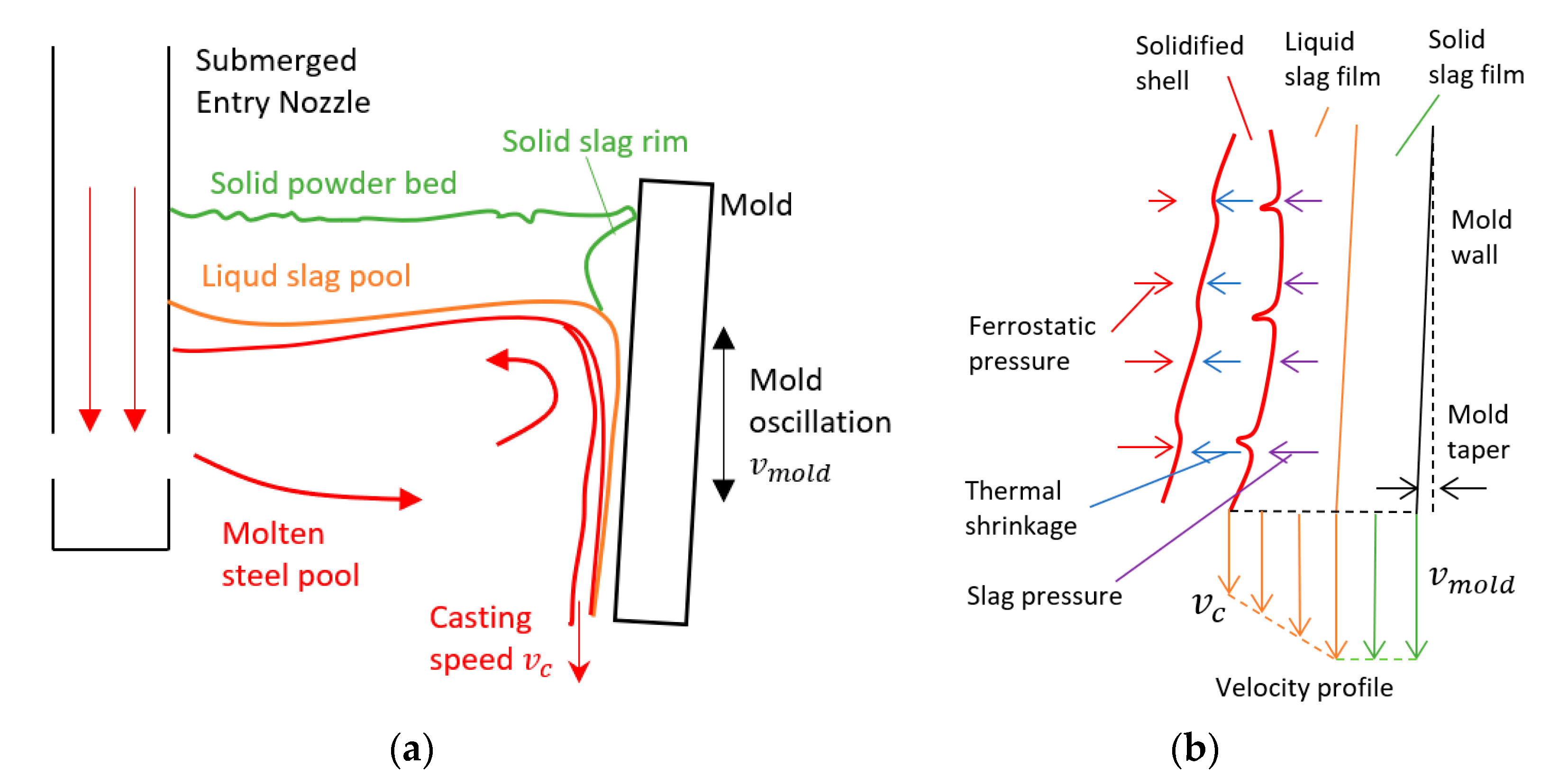
Among the several roles of casting power during continuous casting, providing lubrication between mold and solidified steel shell is crucial since it affects the casting process and surface quality directly. The formation of slag film in the process is described in Figure 1a. The liquid and solid slag supplied from the slag pool and powder bed are infiltrated into the gap between mold and shell while the shell is withdrawn into the casting direction. It is known that mold oscillation is the key to keep the stable infiltration of slag film during the withdrawal. Figure 1b shows more details of the slag film in the gap. As shown in the figure, the infiltrated liquid slag film is the only liquid phase which can offer lubrication between solid phases. Therefore, deep penetration of the liquid slag film as well as higher slag consumption is preferred in the casting process.

The prediction of slag infiltration requires two components, slag film thickness and velocity profile of the slag film (Figure 1b). As a multidisciplinary approach is required for the estimation of slag film thickness (or mold–strand gap), analytical models typically require the thickness as an external input. Several methods have been proposed to calculate the film thickness separately such as using a vibration theory [11,12], Bikerman equation [19], coupling with heat transfer [4,13], and so on. Despite analytical models cannot offer the whole picture of slag infiltration, it gives a useful insight for slag film pressure. In addition to the role as a lubricant to avoid solid–solid contact, the liquid slag film is expected to generate positive pressure against compression between shell and mold (resulting from the thermo-mechanical interaction between thermal shrinkage, mold taper, and ferrostatic pressure) to open the gap [14] as shown in Figure 1b. Physically, the liquid film needs to be squeezed into the flow direction to generate positive pressure against compression. This implies that the profile of liquid film thickness is likely to have a slope rather than being parallel into the casting direction, but it does not indicate the sign of inclination because the mold wall oscillates vertically. In other words, mold oscillation allows continuous casting to adapt to both scenarios that the liquid film channel (1) diverges into the casting direction [7,8,11,12,13,19] or (2) converges into the casting direction [4,14,18,20].

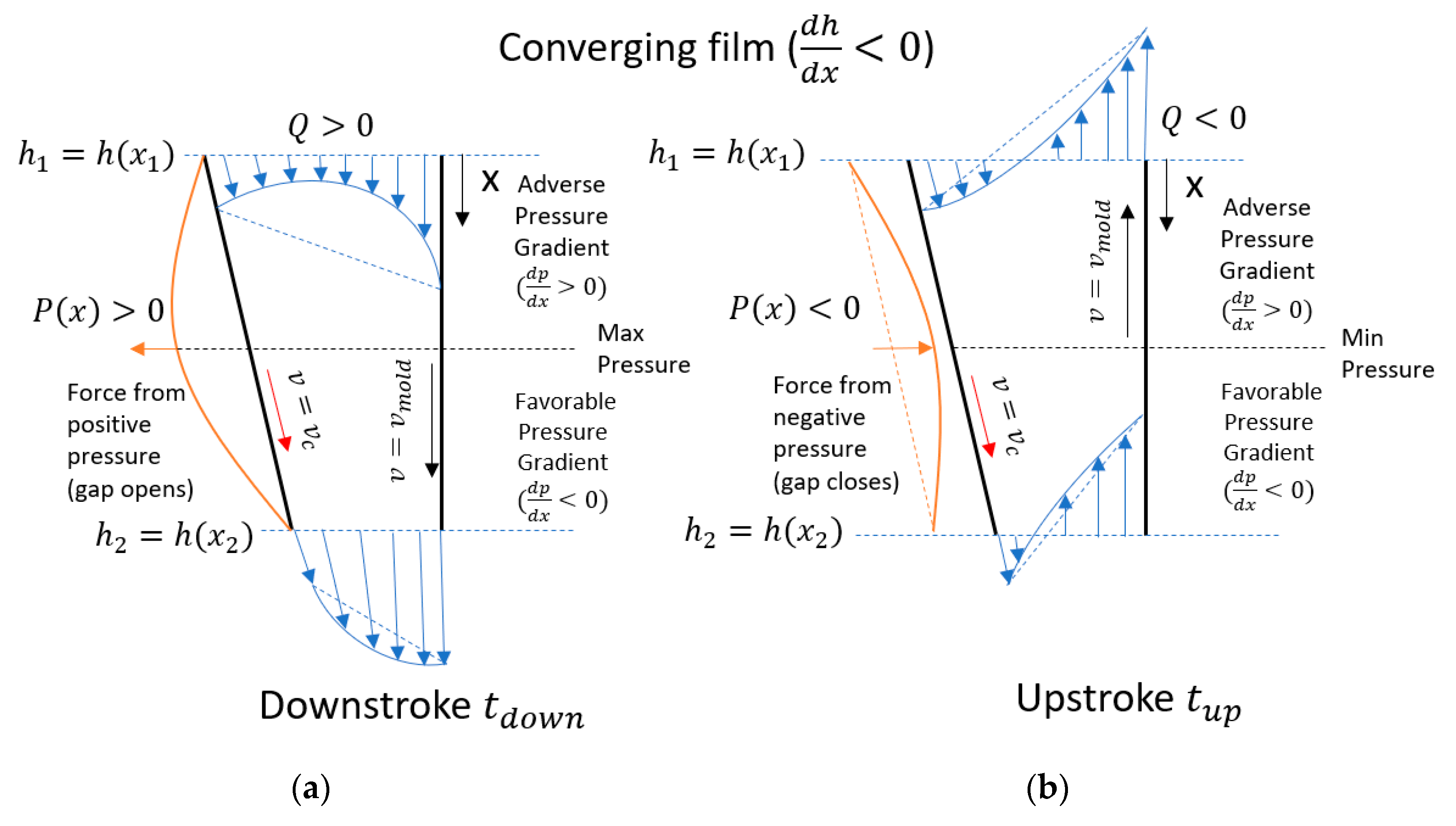
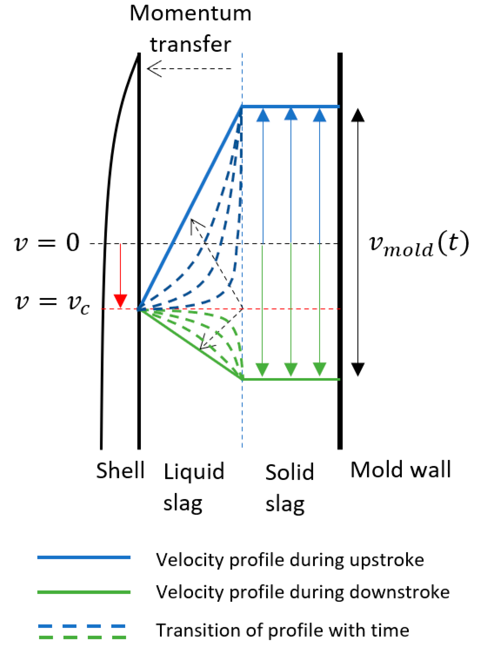
In the case of converging liquid film into the casting direction, positive pressure is generated mostly during the Negative Strip Time (NST) or downstroke of mold oscillation more precisely according to the lubrication theory (Figure 2a): The slag flow dragged by both walls (shell and mold) into the narrowing gap builds up positive pressure and it widens the gap. This is ideal for the slag infiltration because the liquid slag flowing into the casting direction reaches its peak when the gap widens during the NST. On the other hand, negative pressure develops during the upstroke $t_{up}$ (Figure 2b) when the slag flow rate $Q$ becomes negative (i.e., $\left|v_{mold}\right|>\left|v_c\right|$). Naturally, this leads to the closing of mold–strand gap.

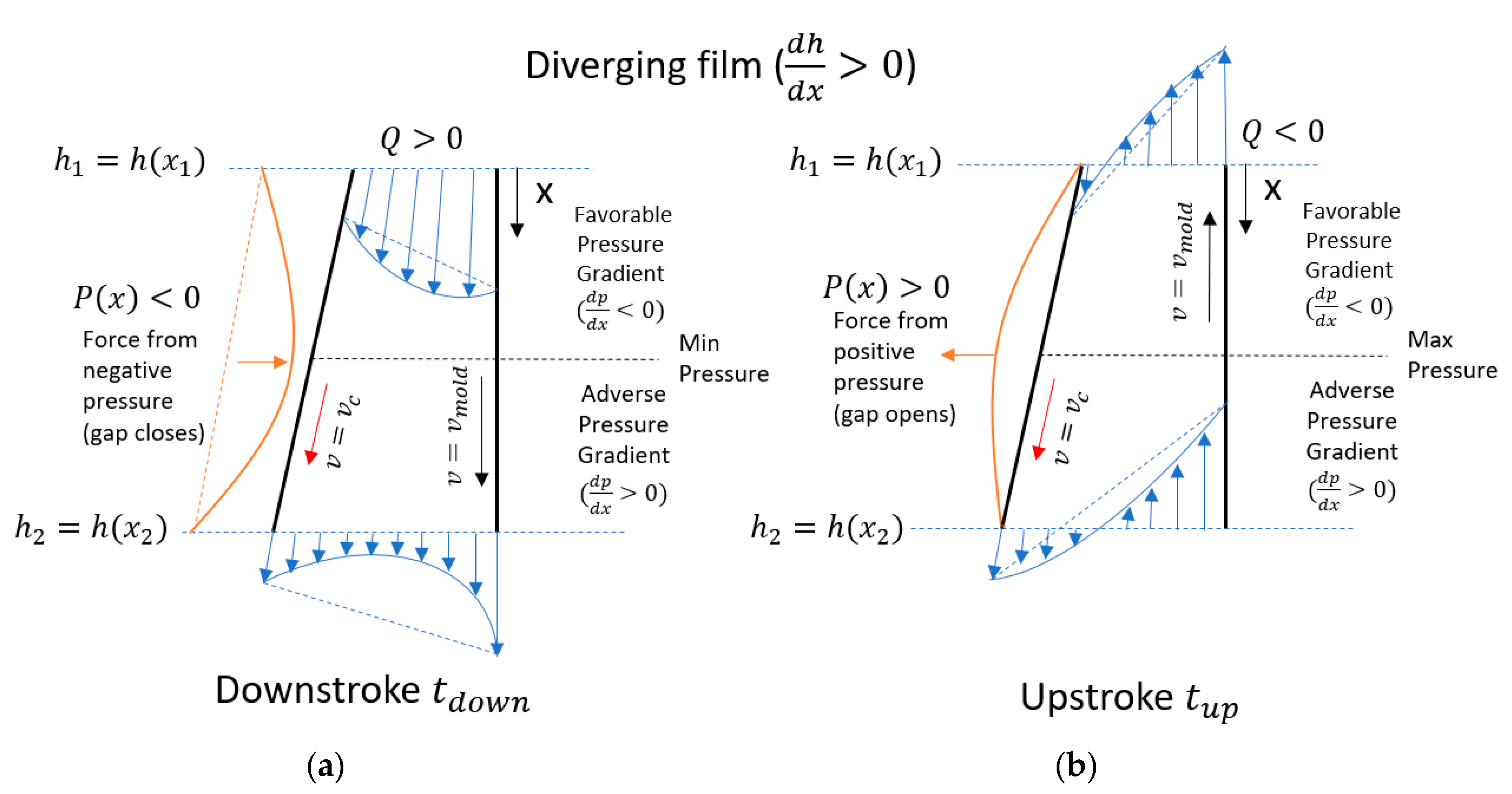
Compared to the converging film, positive pressure develops during the Positive Strip Time (PST) or upstroke of mold oscillation in the scenario of diverging liquid film (Figure 3b): The slag flow is squeezed in the channel when the slag flow rate $Q$ becomes negative. For the negative flow rate $Q$, the flow driven upward by the mold wall needs to be greater than the flow driven downward by the solidified shell. Therefore, the mold wall velocity must be higher than the casting speed to create positive pressure in this scenario. The diverging liquid film is not as favorable as the converging liquid film in terms of infiltration because the liquid film shrinks during the NST when the positive slag flow ($Q$ > 0) is maximized due to the negative pressure developed in the gap (Figure 3a). When the flow is squeezed by approaching two walls in both scenarios (e.g., downstroke with converging film in Figure 2a or upstroke with diverging film in Figure 3b), the positive peak pressure in the film channel pushes the slag away to both ends of the channel that correspond to the meniscus and end of the liquid film channel. Pressure gradients formed by the positive pressure generate a flow against the wall-driven-flow in the wider side of gap (i.e., Adverse Pressure Gradient), but promote the flow in the narrower side (i.e., Favorable Pressure Gradient). On the other hand, the generated negative pressure during the upstroke with converging film (Figure 2b) or the downstroke with diverging film (Figure 3a) sucks the slag from both ends. Accordingly, the opposite direction of pressure-driven flow is generated compared to the cases with positive pressure.

In the slag film channel, there are two different kinds of driving forces that infiltrate the liquid film into the gap: (1) Shell motion (i.e., casting speed) and mold oscillation (i.e., wave shape, stroke, and frequency), (2) gravity and pressure gradient in the gap. From the first driving forces, a wall-driven flow is expected: The steady motion of solidified shell generates a flow such as a Couette flow while the oscillating motion of mold wall drives a Stokes’-2nd-problem-typed flow. When a constant viscosity is assumed, a linear velocity profile develops between the oscillating mold velocity and the steady shell velocity if the viscous effect is dominant, otherwise, some non-linear profile appears depending on the film thickness, kinematic viscosity of slag, and mold frequency. This transient effect results in a transition of the velocity profile due to the oscillatory motion of mold wall (Figure 4).

In addition to the wall-driven flow, the gravity and pressure gradient generate a pressure-driven flow (so-called, Poiseuille flow). This type of flow typically shows a parabolic velocity profile with its peak in the middle such as the velocity profiles shown in Figure 2 and Figure 3. As explained above with the figures, the pressure gradients are developed in the gap by the continuity effect in cases that the film channel has a slope (e.g., diverging or converging film): The film pressure varies locally to satisfy the constant flow rate Q in the film so that the flow driven by pressure gradients makes up for the change of thickness. Therefore, the magnitude of pressure gradient is determined by how much the film thickness decreases or increases between inlet and outlet (i.e., $h_1/h_2$ in Figure 2 and Figure 3).

It is crucial to consider these wall-driven and pressure-driven flows together to predict the slag behavior accurately. For example, from the fact that the thickness of liquid slag film decreases near the meniscus (i.e., converging film), positive pressure develops during NST but negative pressure during PST. Therefore, some counter-intuitive behavior such as positive and higher consumption during PST could be explained by periodic suction (during PST) and overflow (during NST) if the magnitude of pressure-driven flow is comparable to the wall-driven flow.

In the current study, the analytical model focuses on the transient velocity and pressure of slag film with a certain slope. The slope is calculated from a force balance between liquid film pressure and compression in the mold–strand gap. Therefore, the model can predict both scenarios (converging and diverging film channel) based on the compression applied to the mold–strand gap. The ferrostatic pressure is used for the compression under the assumption that the ferrostatic pressure fully transmits to the solidified shell, which is a possible scenario in the real process [14]. The slag film thickness is calculated from measurement data of casting powder consumption. Therefore, the film thickness has a spatial variation based on the calculated slope but static in time.

3. Description of the Model

As the slag flow in mold–strand gap can be described by a combination of Couette flow $u_{couette}$, Stoke’s second problem typed flow $u_{stokes}$, and Poiseuille flow $u_{poiseuille}$, the velocity profile of slag film $u_{total}$ is obtained by the superposition of analytical solutions as follows:

$$u_{total}=u_{couette}+u_{poiseuille }+{\displaystyle \sum }{u}_{stokes}$$

(1)

$$u_{couette}=\frac{u_c}{h}y$$

(2)

$$u_{poiseuille}=\frac{1}{2\mu }\left(\frac{dP}{dx} - \rho g\right)\left(y^2 - hy\right)$$

(3)

$$u_{stokes}=u_{stoke{s}_t}+u_{stoke{s}_s}$$

(4)

$$u_{stoke{s}_t}\left(Y,\tau \right)=\omega h\frac{R_0}{R}{\displaystyle \sum }_{n=1}^{\infty }\frac{F_1\left(j_n,Y\right)}{F_2\left(j_n\right)}\exp \left( - \frac{j_n^2\tau }{R}\right)$$

(5)

$$\begin{array}{cc}{u}_{stoke{s}_s}\left(Y,\tau \right)=& \omega h{R}_0( - \frac{\left(M_1{M}_3+M_2{M}_4\right)\left(f_1\left(Y\right)\sin \left(\tau \right)+f_2\left(Y\right)\cos \left(\tau \right)\right)}{M_3^2+M_4^2}\\ & -\frac{\left(M_1{M}_4 - M_2{M}_3\right)\left(f_2\left(Y\right)\sin \left(\tau \right) - f_1\left(Y\right)\cos \left(\tau \right)\right)}{M_3^2+M_4^2}\\ & +\frac{\left(M_3{M}_5+M_4{M}_6\right)\left(f_3\left(Y\right)\sin \left(\tau \right)+f_4\left(Y\right)\cos \left(\tau \right)\right)}{M_3^2+M_4^2}\\ & +\frac{\left(M_3{M}_6 - M_4{M}_5\right)\left(f_3\left(Y\right)\cos \left(\tau \right)-f_4\left(Y\right)\sin \left(\tau \right)\right)}{M_3^2+M_4^2})\end{array}$$

(6)

$$\begin{array}{cc}{F}_1\left(j_n,Y\right)& =\sin \left(j_n\right)\cos \left(j_{n}Y\right)-\cos \left(j_n\right)\sin \left(j_{n}Y\right)\\ & F_2\left(j_n,Y\right)=-\left(\frac{j_n^4}{R^2}+1\right)\frac{\cos \left(j_n\right)}{2j_n}\end{array}$$

(7)

$$\begin{array}{cc}{f}_1\left(Y\right)& =\sinh \left(\sqrt{\frac{R}{2}}Y\right)\cos \left(\sqrt{\frac{R}{2}}Y\right), f_2\left(Y\right)=\cosh \left(\sqrt{\frac{R}{2}}Y\right)\sin \left(\sqrt{\frac{R}{2}}Y\right)\\ f_3\left(Y\right)& =\cosh \left(\sqrt{\frac{R}{2}}Y\right)\cos \left(\sqrt{\frac{R}{2}}Y\right), f_4\left(Y\right)=\sinh \left(\sqrt{\frac{R}{2}}Y\right)\sin \left(\sqrt{\frac{R}{2}}Y\right)\\ & M_1=\cosh \left(\sqrt{\frac{R}{2}}\right)\cos \left(\sqrt{\frac{R}{2}}\right), M_2=\sinh \left(\sqrt{\frac{R}{2}}\right)\sin \left(\sqrt{\frac{R}{2}}\right)\\ & M_3=\sinh \left(\sqrt{\frac{R}{2}}\right)\cos \left(\sqrt{\frac{R}{2}}\right), M_4=\cosh \left(\sqrt{\frac{R}{2}}\right)\sin \left(\sqrt{\frac{R}{2}}\right)\\ & M_5=\sinh \left(\sqrt{\frac{R}{2}}\right)\cos \left(\sqrt{\frac{R}{2}}\right), M_6=\cosh \left(\sqrt{\frac{R}{2}}\right)\sin \left(\sqrt{\frac{R}{2}}\right)\end{array}$$

(8)

where,

$$\tau =\omega t, \omega =2\pi f, U=\frac{u}{\omega h}, Y=\frac{y}{h}, R=\frac{h^2\omega }{v}, R_0=\frac{u_m}{\omega h}, j_n=n\pi \left(n=\pm 1, 2, 3\dots \right)$$

(9)

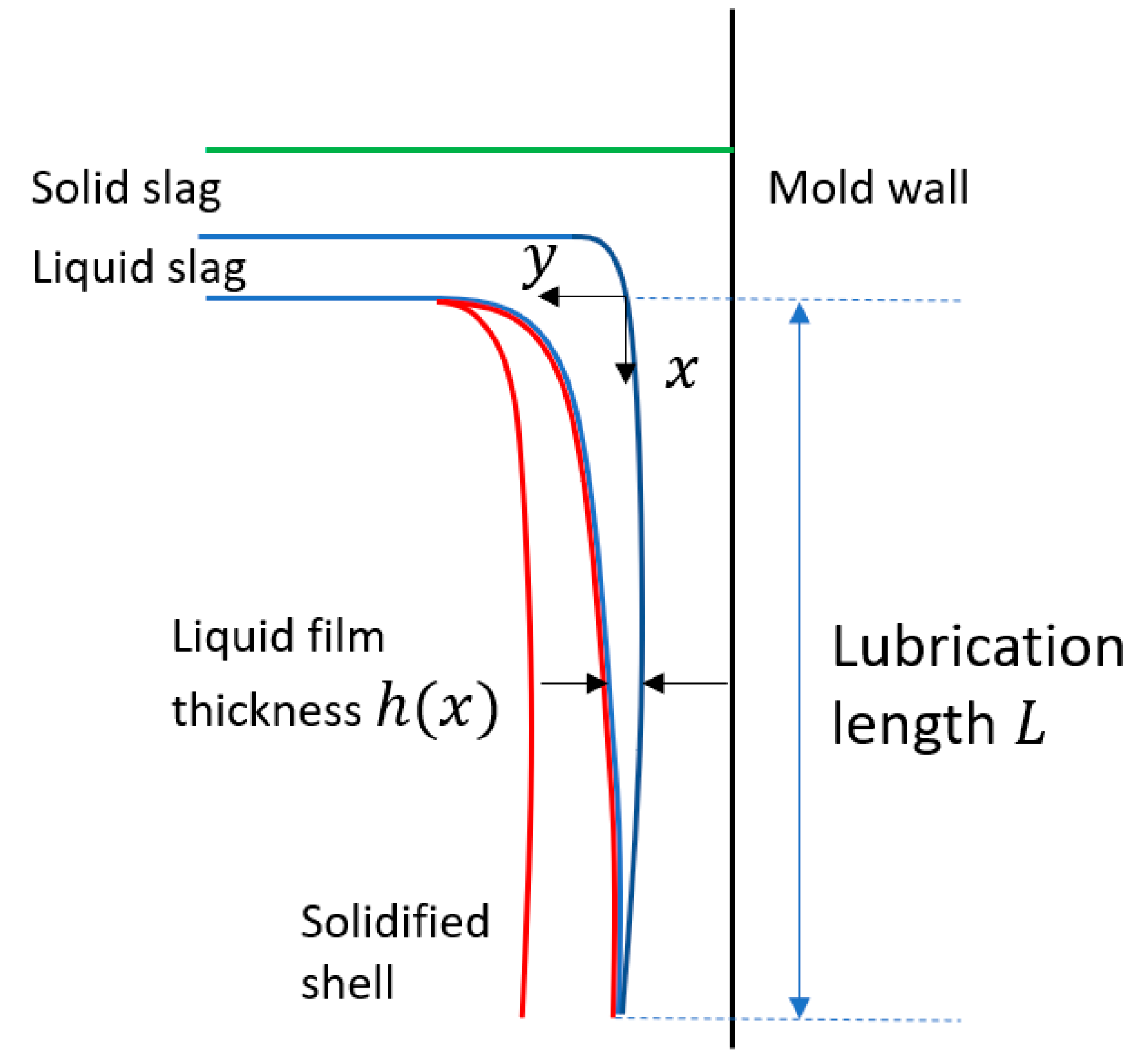
Figure 5 describes the schematic of simulation domain with its coordinate system.

The superposition principle (Equation (1)) is valid since the governing equation is linear mathematically. The transient displacement $y_m$ and velocity of mold wall $u_m$ are obtained from the equations below [28] based on oscillation settings such as amplitude $a_m$ and angular frequency $\omega \left(\omega =2\pi f\right)$:

$$y_m=a_m\sin (\omega t-C_1\sin \left(\omega t+C_2\sin \left(\omega t\right)\right)$$

(10)

$$\begin{array}{cc}{u}_m=a_m\{\omega & -C_1\cos \left(\omega t+C_2\sin \left(\omega t\right)\right)\left(\omega +C_2\omega cos\left(\omega t\right)\right)\}\\ & \cos \left(\omega t-C_1\sin \left(\omega t+C_2\sin \left(\omega t\right)\right)\right).\end{array}$$

(11)

The coefficients $C_1$ and $C_2$ are fitting parameters for non-sinusoidal mold oscillation. The equations converge to sinusoidal oscillation when $C_1=C_2=0$.

As the analytical solution $u_{stokes}$ is for sinusoidal oscillation ($u_m=a_m\omega \sin \left(\omega t\right)$), Fourier expansion is implemented to approximate a non-sinusoidal wave to a sum of multiple sinusoidal waves in cases of non-sinusoidal mold oscillation:

$$u_m\left(t\right)\cong \frac{a_1}{2}+{\displaystyle \sum }_{n=2}^{11}{a}_n\cos \left(\left(n-1\right)\omega t\right)+{\displaystyle \sum }_{m=1}^{10}{b}_m\sin \left(m\omega t\right)$$

(12)

In this study, ten cosine and ten sine functions are used for the approximation. An advantage of using the Fourier expansion is that any kind of periodic function can be approximated into a sum of sinusoidal functions. In real scenarios with an industrial mold oscillator, a conversion of a sampled mold velocity from the oscillator into a mathematical form $u_m\left(t\right)$ using Equation (11) is required in cases that a periodic function for the mold oscillation is not available. After the approximation through Fourier expansion, the analytical solution for $u_{stokes}$ with each sinusoidal oscillation is superposed (i.e., ${\displaystyle \sum }{u}_{stokes}$) to obtain the flow driven by non-sinusoidal mold oscillation. The pressure gradient $\frac{\partial P}{\partial x}$ in $u_{poiseuille}$ is obtained separately from the equation derived from the Reynolds equation below [11]:

$$\frac{\partial P}{\partial x}=\frac{12\mu }{\rho h^3}\left(\frac{\rho }{2}\left(u_m+u_c\right)h+C\right)+\rho g$$

(13)

$$C=\frac{\rho }{12\mu f_2\left(L\right)}[P_1-P_0-\rho gL-6\mu \left(u_m+u_c\right)f_1\left(L\right)$$

(14)

$$f_1\left(x\right)={{\displaystyle \int }}_0^x\frac{dx}{h^2}, f_2\left(x\right)={{\displaystyle \int }}_0^x\frac{dx}{h^3}.$$

(15)

Here, a static film thickness h which has a spatial variation in x (casting direction) is assumed as follows:

$$h\left(x\right)=s\left(x-\frac{L}{2}\right)+h_{avg}$$

(16)

where, $s$ is the slope of the film, $L$ is the lubrication length, and $h_{avg}$ is the slag film thickness at the middle of lubrication length (x = L/2). The pressure gradient term includes the continuity effect from slope and pressure difference between inlet $P_0=P\left(x=0\right)$ and outlet $P_1=P\left(x=L\right)$ of the slag film channel. In cases of no slope (i.e., parallel slag film and h=const), the pressure gradient converges simply to $\left(P_1-P_0\right)/L$. The inlet pressure $P_0$ is calculated based on the depth of slag pool, and the outlet pressure $P_1$ is assumed to be zero. Equations (1)–(8) are solved with boundary conditions below:

At y = 0 (contact with solid slag)

$$u=u_m\left(t\right)$$

(17)

At y = 1 (contact with solidified shell)

$$u=u_c.$$

(18)

The static motion of solidified shell with casting speed $u_c$ drives a linear velocity profile across the film as shown in Equation (2), while the gravity and pressure gradient produce a parabolic flow with its peak at the center of film thickness as described in Equation (3). The oscillatory motion of mold wall generates an unsteady flow which profile can vary between linear and non-linear depending on the relation between momentum transfer, film thickness, and frequency. The final flow $u_{total}$ obtained from the summation of three flows (Equation (1)) representing the viscous effect $u_{couette}$, pressure gradient effect $u_{Poiseuille }$ and transient effect $u_{stokes}$ result in diverse velocity profiles depending on the contribution of each flow.

The flow chart shown in Figure 6 explains the algorithm of analytical model. Firstly, the oscillating mold wall velocity is obtained based on an industrial oscillation setting. In cases of non-sinusoidal mold oscillation, the fitting parameters ($C_1$ and $C_2$ in Equations (10) and (11)) are tuned to get a certain modification ratio $\alpha$ or targeted PST. After that, the mold oscillation velocity described by Equation (11) is approximated to a summation of sinusoidal waves (Equation (12)) through Fourier expansion. Next, based on the externally given slag film thickness h and an initially guessed slope s, the steady flow ($u_{couette})$ is calculated from the analytical solution (Equation (2)). Then, the unsteady flows $({\displaystyle \sum }{u}_{stokes} and u_{Poiseuille}$) are calculated with a certain time step. The pressure gradient term is obtained based on the transient mold wall velocity $u_m$ as well as slope of the channel (Equation (13)). At every time step, all the flow solutions are summed to obtain the final velocity profile ($u_{total}=u_{couette}+u_{Poiseuille }+{\displaystyle \sum }{u}_{stokes}$). Transient slag consumption and force from film pressure are obtained based on the transient pressure and velocity profiles. After that, a time-averaged force from film pressure is compared to compression from ferrostatic pressure ($F={{\displaystyle \int }}_0^L{\rho }_{steel}gx dx)$, and the loop is iterated to find a proper slope $s$ until the time-averaged force balances the compression.

4. Validation of the Model

The analytical model is tested with measurement data from plant trials in Shin et al. [2]. Predicted slag consumption is compared to the measured powder consumption for the validation. The analytical model requires a liquid slag film thickness $h$ as an input. Several assumptions are made to estimate the thickness from the measurement data. Firstly, the solid slag film is assumed to be attached to the mold wall. In other words, liquid slag only contributes to slag consumption. Secondly, the net slag consumption per cycle from $u_{stokes}$ is assumed to be zero from the fact that it drives a periodic flow. Under these assumptions, the slag consumption can be calculated by the equations below from the analytical solutions for $u_{couette}$ (Equation (2)) and $u_{poiseuille}$ (Equation (3)):

$$Q_m=\left(\frac{u_{c}h}{2}+\frac{\rho g{h}^3}{12\mu }-\frac{h^3}{12\mu }\frac{dP}{dx} \right)\times \rho \times 2\left(W+H\right)$$

(19)

$$Q_{lub}=\frac{Q_m}{u_c\times 2\left(W+H\right)}=\frac{\rho h}{2}+\frac{{\rho }^{2}g{h}^3}{12\mu u_c}-\frac{\rho h^3}{12\mu u_c}\frac{dp}{dx}$$

(20)

where the $Q_m$ is the mass flow rate of slag film $\left(\mathrm{kg}/\mathrm{s}\right)$, the $Q_{lub}$ is the slag consumption per steel surface area $\left(\mathrm{kg}/{\mathrm{m}}^2\right)$. There are three terms contributing to the slag consumption $Q_m$: $\frac{u_{c}h}{2}$ term from steady shell motion $V_c$, $\frac{\rho g{h}^3}{12\mu }$ term from gravity, $-\frac{h^3}{12\mu }\frac{dp}{dx}$ term from pressure gradient. One thing worth mentioning here is the relationship between consumption and casting speed $u_c$. As shown in Equation (19), the slag consumption $Q_m$ seems increasing with casting speed $u_c$ due to the contribution of $u_{couette}$ ($\frac{u_{c}h}{2}$ term) but decreasing with viscosity by the other terms. On the other hand, the relation in inverse-proportion between slag consumption and casting speed or viscosity appears in the definition of $Q_{lub}$ by the terms associated with gravity and pressure gradient. However, the prediction of slag consumption is not as explicit as it appears in the equations since the film thickness h is a function of casting speed $u_c$. Therefore, it is not a complete solution unless the relationship between casting speed $u_c$ and film thickness h is given by another model, although the analytical solution can predict the same consumption trend to real casters such as less consumption $Q_{lub}$ with higher casting speed $V_c$ or viscosity $\mu$ to some extent. The formula for slag consumption (Equation (20)) can be simplified further to $Q_{lub}\cong \frac{\rho h}{2}$ when the slag film is very thin (h << 1). This means that the contribution of pressure-driven flows (gravity and pressure gradient) diminishes as the film becomes thinner and the consumption is determined by solidified shell motion ($\frac{u_{c}h}{2}$ term from $u_{couette}$). From the simplified formula $Q_{lub}$, the liquid slag film thickness can be estimated by

$$h_{avg}\cong \frac{2Q_{lub}}{\rho }.$$

(21)

This simplified equation is used to calculate the liquid film thickness $h_{avg}$ (in Equation (16)) from the casting powder consumption in Shin et al. [2].

Table 1. Operating conditions from plant trials (Shin et al. [2]).

Case	Mold Width (mm)	Casting Speed (m/min)	Oscillation Stroke (mm)	Oscillation Frequency (Hz)	Modification Ratio (%)	NST (s)	PST (s)	Powder Consumption ${\mathit{Q}}_{\mathit{l}\mathit{u}\mathit{b}}$  $(\mathbf{k}\mathbf{g}/{\mathbf{m}}^2)$
A1	1300	1.464	6.44	2.65	24	0.107	0.270	0.247
A2	1300	1.458	5.00	2.43	0	0.115	0.296	0.232
A3	1300	1.47	5.00	2.94	12	0.100	0.241	0.225
A4	1300	1.494	5.00	3.49	24	0.081	0.205	0.253
A5	1300	1.5	6.00	2.08	12	0.127	0.353	0.223
A6	1300	1.47	6.00	2.45	24	0.110	0.299	0.229
A7	1300	1.488	6.00	2.90	0	0.121	0.224	0.230
A8	1300	1.488	7.00	1.77	24	0.139	0.426	0.248
A9	1300	1.5	7.00	2.09	0	0.154	0.324	0.208
A10	1300	1.494	7.00	2.49	12	0.126	0.276	0.211
B1	1570	1.35	6.25	2.46	24	0.114	0.292	0.271
B2	1570	1.38	6.30	2.52	24	0.112	0.285	0.247
B3	1570	1.422	6.37	2.58	24	0.109	0.278	0.256
B4	1300	1.482	6.47	2.69	24	0.106	0.267	0.238
B5	1300	1.476	6.46	2.67	24	0.106	0.268	0.237
B6	1300	1.518	6.53	2.74	24	0.104	0.261	0.215
B7	1300	1.548	6.58	2.79	24	0.102	0.256	0.212
B8	1050	1.65	6.75	2.96	24	0.097	0.241	0.210
B9	1050	1.662	6.77	2.97	24	0.097	0.240	0.194
B10	1300	1.464	6.44	2.66	24	0.107	0.270	0.247
B11	1300	1.5	6.50	2.71	24	0.105	0.264	0.234

shows the operating conditions used in the plant trials [2] and measured powder consumptions. Calculations for 20 different cases including three oscillation modes (sinusoidal and non-sinusoidal oscillation with two modification ratios, $\alpha =12\% \mathrm{and} 24\%$) are compared to the measurement data. The lubrication length of liquid slag film is assumed to L = 0.1 m. The same slag properties used in Shin et al. [2] (slag density $\rho =2680 \mathrm{kg}/{\mathrm{m}}^3$, slag viscosity $\mu =0.321 \mathrm{Pas}$) are applied in the calculations.

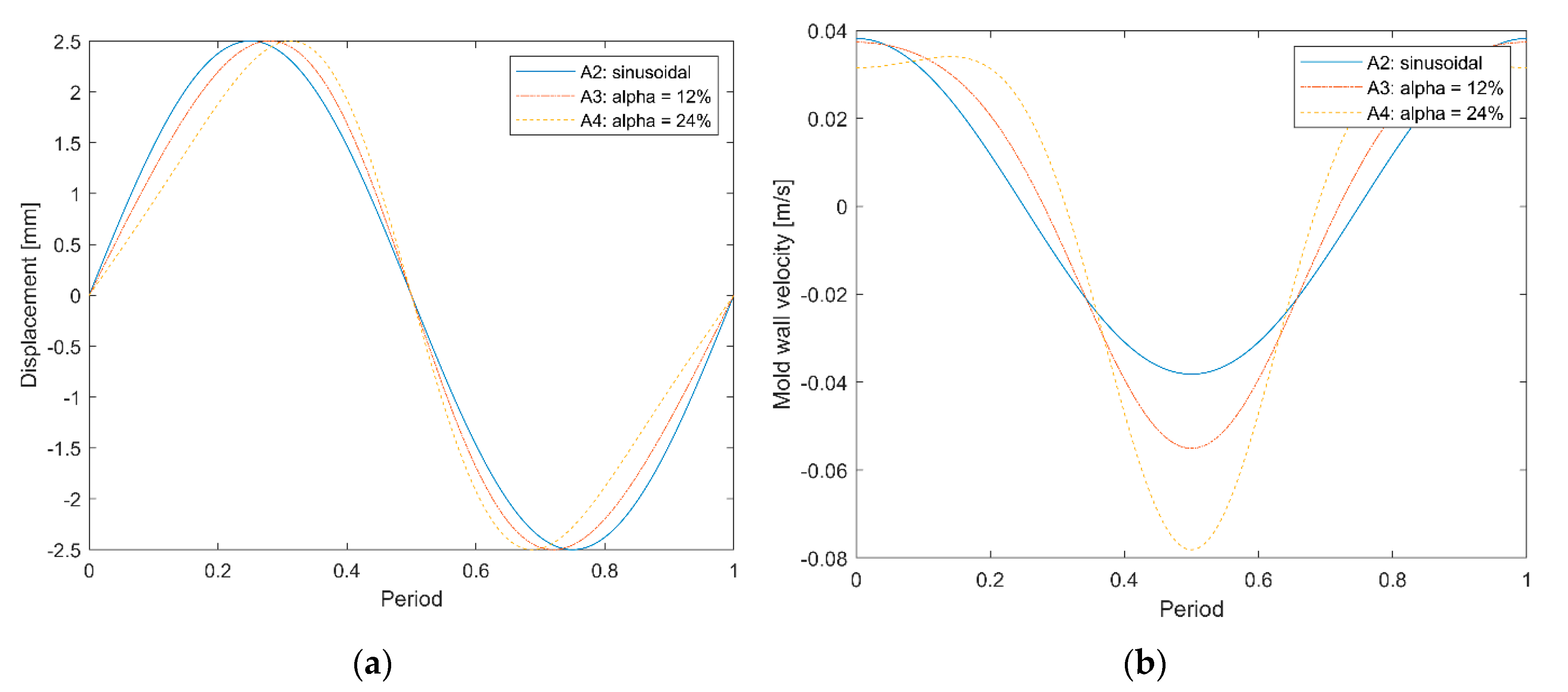
Figure 7 visualizes mold displacement and velocity for Case A2 (sinusoidal), A3 ($\alpha =12\%),$ and A4 ($\alpha =24\%)$ calculated by Equations (10) and (11). It shows a clear trend from Figure 7b that the NST becomes narrower but the descending velocity becomes faster as the modification ratio increases.

With the calculated mold wall velocities (Figure 7b) as a boundary condition, slag flows in mold–strand gap for Case A2 and A4 are compared in Figure 8. The estimated liquid slag film thicknesses from Equation (21) for A2 and A4 are 173 $\mathsf{\mu }\mathrm{m}$ and 189 $\mathsf{\mu }\mathrm{m}$ respectively. Here, y = 0 is the mold wall or solid slag layer fully attached to the mold wall, and y = 1 is the solidified shell. The calculated velocity profiles at the center of film channel (x = L/2) are almost linear during the oscillation cycle. This means that the influences of gravity and pressure gradient are imperceptible in the thin film thickness used in the calculations as assumed in the derivation of Equation (21). Namely, the formula to calculate liquid film thickness from slag consumption $h\cong \frac{2Q_{lub}}{\rho }$ is valid with thickness h < ~200 μm, which falls into a typical range of liquid film thickness observed in continuous casting [22]. Also, any transient effects such as the transition of velocity profile (Figure 4) are not clearly observed in the results and the entire velocity profile responds quickly to the mold oscillation. Thus, the viscous effect dominates the overall slag flow due to its thin film thickness.

Figure 9 shows the difference of velocity profiles between top (x = 0) and bottom (x = L) of the film channel during the oscillation cycle in Case A2.

Compared to the velocity profile obtained at the center (x = L/2), they show parabolic profiles by the continuity effect as described in Figure 2 and Figure 3. Because of the converging film (s = −4.75 × 10⁻⁴) which slope is calculated from the force balance through iterations (Figure 6), positive pressure develops during the downstroke period $t_{down}$ and it pushes the slag flow to both ends (e.g., t = 3T/8 or t = 4T/8). This continuity or pressure gradient effect promotes the flow at the bottom of slag channel (x = L) but interrupts the flow at the top (x = 0) by bending the velocity profile to parabolic shapes with opposite directions depending on the location. The same mechanism is applicable for explaining the flow during the upstroke period $t_{up}$ with negative pressure (e.g., t = 0).

The transient slag consumption and force from slag pressure for Case A2, A3, and A4 are shown in Figure 10. Both profiles show a similar trend with regards to the modification ratio: The distribution of both curves becomes sharper as the modification ratio increases, which corresponds to the mold wall velocity in Figure 7. Also, both reach their peak during the NST but the lowest negative consumption and force during the PST are obtained with the highest modification ratio (Case A4, $\alpha =24\%$). The calculated net consumptions for A2, A3, and A4 are 0.2285, 0.2219, and 0.2486 $\mathrm{kg}/{\mathrm{m}}^2$, which agree well to the measurement data in Table 1. On the contrary, it shows a small discrepancy in terms of the timing of peak. The slag consumption shows a delay of its peak as the modification ratio increases, while the force responds to the mold velocity precisely so that the maximum force is obtained at t = T/2 when the mold descending velocity is its peak. It is suspected that the transient effect discussed in Figure 4 is responsible for the small delay in consumption. More details of this effect are discussed in Section 5.

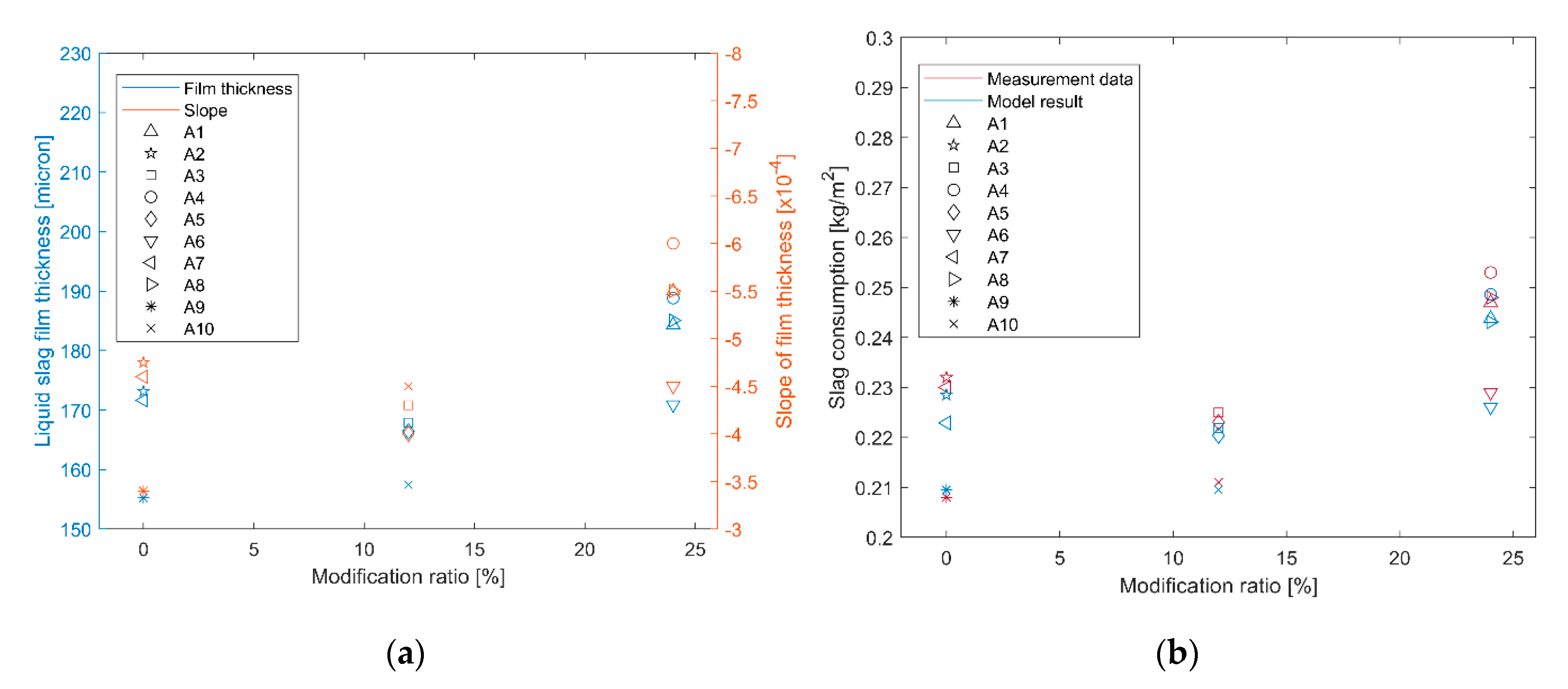
Figure 11 shows the estimated liquid film thickness and slope of the film from the analytical model and comparison of the consumption to the measurement data. The results are plotted with the modification ratio to visualize the effect of non-sinusoidal mold oscillation with Case A1–A10.

The results show a corresponding trend that the liquid film thickness, slope of the film, and slag consumption increase with the modification ratio. All the estimated slopes for slag film are negative to generate a positive force against compression. From the relation that the slag film pressure decreases with film thickness but increases with slope magnitude (Equations (13)–(15)), a steeper slope is obtained with a thicker slag film to generate the same magnitude of force against compression. The calculated consumption also increases with the modification ratio and agrees well with the measurement data.

Figure 12 shows the results for Case B1–B11 to visualize the effect of casting speed by fixing the modification ratio to 24%.

As expected, the calculated slag consumption decreases with casting speed and the same trend is observed between film thickness and slope in the results for Case A1–A10. The calculated slag consumptions show that they match better in cases with higher casting speed because the estimation of slag film thickness becomes more accurate with thinner slag film ($h\cong \frac{2Q_{lub}}{\rho }$ when h << 1), which can be obtained with higher casting speeds as shown in Figure 12a. Namely, other factors such as gravity, pressure gradient, and transient effect start contributing to the slag consumption as the slag film gets thicker. Thus, an advanced model to estimate slag film thickness will be required to improve the accuracy of cases with thick liquid films ($h>200 \mathsf{\mu }\mathrm{m}$).

5. Mechanism of Higher Consumption under Non-Sinusoidal Mold Oscillation

With the validated analytical model, a parametric study is conducted to investigate the influence of non-sinusoidal mold oscillation on slag flow. As discussed in Section 2, slag consumption is determined by slag film thickness h and velocity profile of slag flow u $\left(Q_m=\rho {{\displaystyle \int }}_0^{h}u dy\right)$. Under the same film thickness h (to separate its impact on infiltration), consumption and force from slag pressure are compared between sinusoidal and non-sinusoidal oscillations (modification ratio $\alpha$ up to 36%). The same conditions from Case A2 including oscillation setting (stroke and frequency), casting speed, and slope of the film (s = −4.75 × 10⁻⁴) are assumed (in Table 1) except the modification ratio. The comparison of slag consumption $Q_{lub}$ and force from different modification ratios is shown in Figure 13.

It appears clearly that the consumption and force profiles both reflect the mold wall velocity: They become sharper with higher peaks as the modification ratio increases. However, the slag consumption profile becomes asymmetric as the modification ratio $\alpha$ increases compared to the force profile that shows symmetric distribution regardless of $\alpha$. Interestingly, the slag consumption does not change much with modification ratio $\alpha$ under the same film thickness (h = 173$\mathsf{\mu }\mathrm{m}$): The net consumption $Q_{lub}$ obtained during one cycle is 0.2285 $\mathrm{kg}/{\mathrm{m}}^2$ (sinusoidal), 0.2282 $\mathrm{kg}/{\mathrm{m}}^2$ ($\alpha =0.12)$, 0.228 $\mathrm{kg}/{\mathrm{m}}^2$ ($\alpha =0.24)$, and 0.2279 $\mathrm{kg}/{\mathrm{m}}^2$ ($\alpha =0.36)$. Therefore, this reveals that non-sinusoidal mold oscillation does not increase infiltration through slag flow velocity u. On the contrary, the time-averaged force from slag pressure increases with modification ratio: 381.20 $\mathrm{N}/\mathrm{m}$ (sinusoidal), 383.40 $\mathrm{N}/\mathrm{m}$ ($\alpha =0.12)$, 385.83 $\mathrm{N}/\mathrm{m}$ ($\alpha =0.24)$, and 386.55 $\mathrm{N}/\mathrm{m}$ ($\alpha =0.36)$. Also, the generated force during the PST increases with $\alpha$ and becomes positive during the entire PST when $\alpha \ge 0.24$. Therefore, this implies that non-sinusoidal mold oscillation increases slag infiltration through film thickness by generating longer positive pressure during PST and higher peak pressure during NST. A coupling with a separate model to calculate transient slag film thickness based on the force from slag pressure will be required for more quantitative analysis.

6. Timing of Slag Consumption

The validated analytical model is now applied to the meniscus region to investigate the timing of slag consumption. Instead of using Equation (21) and iterations to estimate the film thickness and slope, they are assumed to $h_1$ = 2 mm with slope s = −0.0033, which are externally given based on previous 2D model calculations [29]. The Fourier number is used as an indicator to quantify the relationship between momentum transfer, slag film thickness, and mold oscillation frequency discussed in Figure 4. The Fourier number is defined as follows:

$$Fo=\frac{\upsilon t}{L^2}$$

(22)

where, $\upsilon$ is the kinematic viscosity of slag ($\upsilon =\frac{\mu }{\rho }$), $t$ is the characteristic time, $L$ is the characteristic length. Here, the period of mold oscillation ($T=1/f$) and slag film thickness ($h=2 \mathrm{mm}$) are used for the $t$ and $L$ respectively. Note that each Fourier number represents numerous cases that have different combinations of slag viscosity, mold oscillation setting, and slag film thickness. In this parametric study, the kinematic viscosity is used to control the Fourier number. For the mold oscillation setting, conditions from Case A4 (Table 1) are applied.

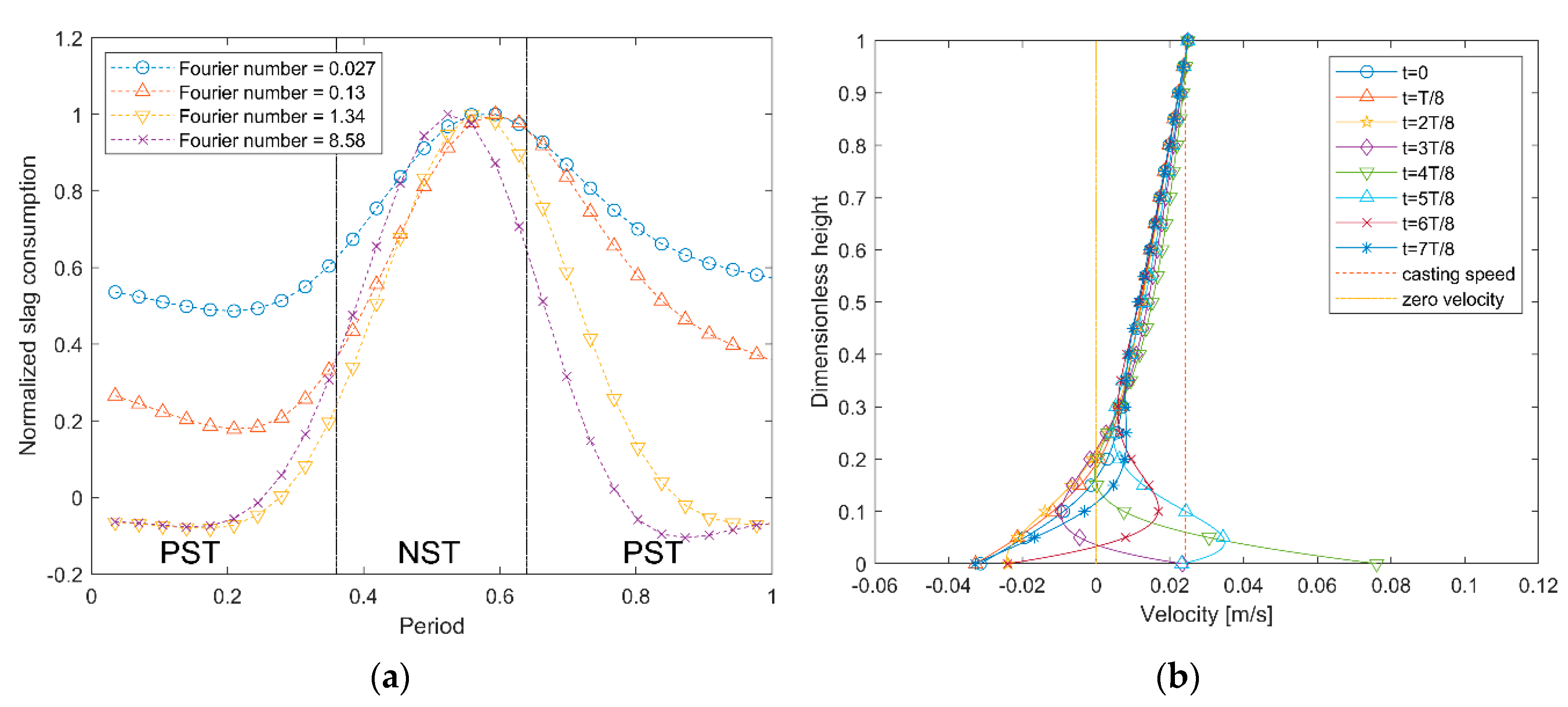
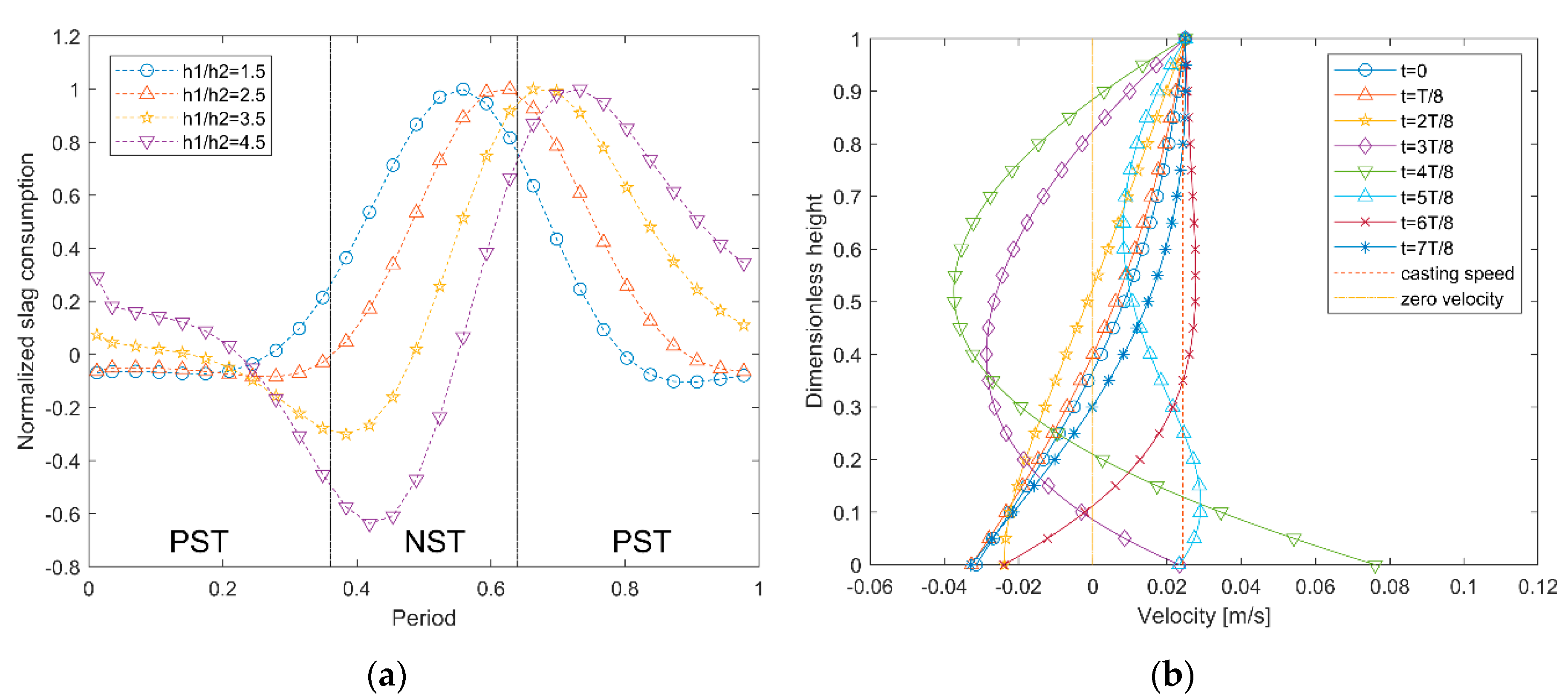
Figure 14 shows the normalized slag consumption with different Fourier numbers and the transient velocity profiles for Fo = 0.027. The slag consumption is normalized to understand the general trend qualitatively.

From the consumption profile in Figure 14a, a delay of peak is observed as the Fourier number decreases: The peak of slag consumption comes after the peak of descending mold velocity (at period = 0.5). A transition of velocity profile due to the slow response of slag flow to mold oscillation generates this kind of delay as shown in Figure 14b near the mold wall (y < 0.3). On the other hand, the force from slag pressure does not show any delay regardless of Fourier number and it responds precisely to the mold oscillation as shown in Figure 10 and Figure 13. Also, the negative consumptions observed during the PST in high Fourier numbers turn to positive and the contribution of PST to the total slag consumption becomes higher as the Fourier number decreases. The transient velocity profiles for $Fo$ = 0.027 show a separation of regions where mold oscillation dominates (y < 0.3), and shell motion dominates (y > 0.3). The mold oscillation dominant region decreases as the Fourier number decreases and the stable positive consumption is obtained from the shell motion dominant region. Consequently, the fluctuation of overall consumption reduces over time, and it flattens the consumption pattern. This phenomenon explains the discrepancy between previous results from numerical models. Some works showed positive consumption during the entire oscillation cycle [17,29] while others showed periodic variation between negative and positive consumption [14,15,18]. According to the results from this parametric study, the consumption pattern depends on the conditions which can be represented by the Fourier number. A thicker slag film with higher mold frequency and lower slag viscosity limit the influence of mold oscillation over the entire film thickness, and the region driven by steady shell motion allows stable positive infiltration as shown in Figure 14b. Accordingly, this results in higher consumption during the PST.

In addition to the transient effect represented by Fourier number, the influence of pressure gradient effect on timing of slag consumption is investigated with different thickness ratios of slag film channel between inlet $h_1=h \left(x=0\right)$ and outlet $h_2=h \left(x=L\right)$. Figure 15 shows the transient consumption during the mold oscillation cycle with different film thickness ratios.

The contribution of pressure-driven flow induced by the continuity effect (discussed in Section 2) increases with the thickness ratio and it turns out to delay the peak of consumption from the peak of descending mold velocity (at period $T$ = 0.5). The results show that the peak is shifted to outside of NST when the thickness ratio becomes greater than $h_1/h_2>2.5$ (in Figure 15a). The transient velocity profiles for $h_1/h_2=4.5$ in Figure 15b visualize parabolic flow patterns against the mold wall velocity: The adverse pressure gradient developing near the inlet in the converging film (e.g., Figure 2a) dominates the flow and generates a backflow (e.g., velocity profile at $t=4T/8$ in Figure 15b). This backflow against the mold wall motion deviates the consumption pattern from the mold oscillation (i.e., the delay of the consumption peak). Similar behavior is reported from 2D numerical model results recently [30]. On the contrary, no delay is observed for the force from slag pressure like the parametric study for transient effect with Fourier number.

Therefore, this implies that there is a time difference between slag consumption and mold–strand gap behavior near the meniscus, which aligns with infiltration mechanisms discussed in previous studies [8,10,12]. The current parametric studies seem to reveal that the time difference (lagging or phase shift) is attributed to the transient effect and pressure gradient effect, according to a fluid mechanics perspective. Compared to the corresponding behavior in thin slag films with sinusoidal oscillations (e.g., Case A2 in Figure 10) that the force and consumption both reach their peak at the maximum descending velocity of mold wall (period $=T/2$), the slag flow starts showing some lagging behavior compared to its pressure as the transient effect (represented by $Fo$) or pressure gradient effect (represented by $h_1/h_2$) increases near the meniscus. Since the mold–strand gap opens and closes based on the slag pressure which precisely responds to the mold oscillation, it naturally gives diverse consumption patterns (timing for peak consumption, ratio of consumption during PST and NST, etc.) depending on the extent of mismatch between the slag pressure and slag flow. Therefore, the consideration of time difference between slag and gap behavior will be important for the optimization of mold oscillation. A coupling with a model for transient mold–strand gap will be necessary to investigate this phenomenon further in the future.

7. Conclusions

A simple but reliable 1D analytical model for slag infiltration is developed to investigate the slope of slag film channel, influence of non-sinusoidal mold oscillation, and timing of slag consumption. The important findings are summarized below:

1

The vertical mold oscillation allows continuous casting to adapt to both scenarios that the liquid film channel diverges or converges into the casting direction. Under a possible scenario that the ferrostatic pressure is fully transmitted (without being canceled by thermal shrinkage), a negative slope for slag film channel (i.e., converging into casting direction) is required to produce positive force against compression from the ferrostatic pressure. The known trends such as higher casting speed with lower slag consumption are obtained with converging films.

2

Model calculations show that non-sinusoidal mold oscillation does not facilitate slag infiltration under a static film thickness. This leads to a hypothesis that higher slag consumption is achieved by increasing slag film thickness through longer positive slag pressure during PST and higher peak pressure during NST. A coupling with a model to estimate transient mold–strand gap will be required to validate this.

3

A time difference is observed near the meniscus between slag consumption and force from slag pressure because of the transient effect (represented by Fourier number $Fo$) and pressure gradient effect (represented by thickness ratio of slag film channel $h_1/h_2$). The slag flow starts showing some lagging behavior compared to its pressure as the two effects dominate the flow. Since the mold–strand gap opens and closes based on the slag pressure which precisely responds to mold oscillation, diverse consumption patterns (timing of peak consumption, ratio of consumption during PST and NST, etc.) are expected depending on the extent of mismatch between slag pressure and slag flow.