Mathematical Development of a Novel Discrete Hip Deformation Algorithm for the In Silico Elasto-Hydrodynamic Lubrication Modelling of Total Hip Replacements

Abstract

In this paper, the procedure to achieve an accurate deformation model of a total hip replacement (THR) was proposed with the aim to obtain a numerical tool to be simply merged into THR elasto-hydrodynamic computational synovial lubrication algorithms. The approach was based on the Finite Element Method (FEM) and was developed in a Matlab code, allowing the definition of the influence matrix and of a boundary conditions vector. It works with linear tetrahedra and performs the displacement calculation for both the acetabular cup and the femoral head, taking into account the anatomical hip relative motion, by coupling them with a cubic interpolation matrix. Two simulations were conducted in order to validate the algorithm and the results were compared with the ones obtained by the commercial software Ansys. The comparison provides a satisfactory agreement in terms of surface deformation, Von Mises stress and strain energy, proving the reliability of the model and the possibility to use the model in the in silico prostheses tribological simulations, avoiding the complexity and the high computational resource requirement coming from the coupling between complex lubrication algorithms and FEM commercial software, and with the possibility to directly act on many key parameter characteristics of the investigated problem.

1. Introduction

In biomechanics, the human joints can be physically modelled as coupled surfaces separated by the lubricant synovial fluid, so the lubrication theory is fundamental to develop numerical algorithms able to predict interesting tribological phenomena, like the joint eccentricity, synovial pressure and thickness, surface wear, etc [1,2,3,4].

The operating conditions in which the lubricated joints operate are represented by the load acting on the joint (dynamics) and the relative motion between the linked bodies (kinematics). Based on the operating conditions, three lubrication modes can be distinguished [5,6,7]:

• When the joint is subjected to intense relative motion and light loading, the hydrodynamic lubrication occurs, so the coupled surfaces are totally separated by the lubricating fluid along the whole contact area;
• The boundary lubrication is established when the high load and the slow relative motion do not allow to obtain the surfaces’ separation, so the lubrication effect is governed by chemical reactions at the contact interface; and the slow relative motion don’t allow to obtain the surfaces’ separation, so the lubrication effect is governed by chemical reactions at the contact interface;
• In the intermediate condition, the load is supported both by asperities in contact and by the lubricating fluid pressure, so it is defined as mixed lubrication.

A particular case of the hydrodynamic mode, the Elasto-Hydrodynamic Lubrication (EHL), occurs when the lubricating fluid pressure is so high that it causes the coupled surfaces’ elastic deformation, guaranteeing the survival of a small gap between the surfaces filled by the synovial fluid even in hard loading conditions. In this case, the calculations of the lubricant’s gap within a numerical lubrication algorithm needs a deformation model able to evaluate the surfaces’ deflection due to fluid pressure [5].

In the framework of human joint replacements, the mechanical behaviour of the implant’s surfaces is determined by the coupled biomaterials and the geometry, so several solutions are available in terms of hard materials (ceramics or metal alloys) and soft materials (polymers). In the particular case of the hip arthroplasty, the implant can be geometrically modelled as a spherical cup for the acetabular component and a sphere for the femoral one.

Nowadays, an accurate description of the global tribological behaviour of the prosthesis surfaces’ interactions is an important research topic, in order to predict with an in silico approach the implant wear due to particular kinematics [8,9]: the loss of material within the prosthesis is strictly related to its duration and, as a consequence, its estimation is necessary to minimize the revision surgical procedures after the first installation.

In a total hip replacement (THR), elasto-hydrodynamic lubrication modelling several deformation models is usually adopted in the solution algorithms. When the hip implant is a type of hard-on-soft prosthesis, the constrained column model can be used in order to neglect the deformation of the harder part (generally the metallic or ceramic femoral head) and to evaluate the dominant deformation of the softer one (the acetabular cup made of polyethylene). This approach consists of the modelling of the local cup deformation as proportional to the local fluid pressure, through constants which depend on the mechanical and geometrical properties of the acetabular cup (Young modulus, Poisson ratio, inner radius and thickness) [10,11,12,13]. An approach similar to the constrained column model is to consider the analysed surface as an Elastic Foundation, in order to keep the independence of the local deformation on the surrounding pressures and obtaining a relationship useful for the contact modelling [14,15,16,17,18,19]. The deformation of other types of implants, composed of materials with comparable Young modulus, cannot be approximated by a spring model (like the constrained column one) because there is not a dominant deflection between the two surfaces and generally the local deformation could not depend only on the local pressure but also on the surroundings of the analysed points. In order to overcome these issues and to model the deformation of linear elastic materials with comparable stiffness, some authors use an equivalent spherical discrete convolution method based on the Fast Fourier Transform of the influence coefficients coming from the theory of the semi-infinite bodies in point contact, while others take advantage of several finite element simulations to build the entire matrix of influence coefficients entry by entry [20,21,22,23].

The aim of this paper is to propose, in the framework of the tribological modelling of a THR, a deformation model based on the finite element approach, able to provide the influence coefficient matrix, which evaluates the surfaces’ deformation, due to a particular pressure field acting on them and which, above all, can be written and run in the same computational environment of more complex lubrication algorithms for the accurate in silico wear assessment of the prostheses. The developed finite element model considers the two whole parts of the hip joint (acetabular cup and femoral head) and the relative motion between them, through a cubic interpolation matrix. In order to validate the model, the results are compared with the ones calculated by the software Ansys, of course for the same problem inputs. The proposal represents a succeeding improvement of previous authors’ works [2,3,4].

2. Materials and Methods

2.1. Finite Element Model

According to the classical finite elements approach, the model is based on the discretization of the analysed volumes in several linear tetrahedra with a regular mesh algorithm. In order to obtain the influence matrix, nodal forces due to the pressure are taken into account through nodal pressures acting on a face of the tetrahedron. With reference to Figure 1, the generic linear tetrahedron, composed of the nodes $I$, $J$, $K$ and $H$, is subjected to the pressure action represented by the nodal pressures $p_I$, $p_J$ and $p_K$ on the respective face with outward-pointing normal $\widehat{\mathit{n}}$ located on the face’s centre $C$.

Starting from the nodal pressures, the relative nodal force vector ${\Phi }_p$ was calculated with the virtual work principle—the virtual work $\delta W_p$ done by the pressure $p$ acting on the tetrahedron’s face which produces a virtual displacement $\partial \mathit{u}$ is given in (1), considering the analysed face area $A$ and the nodal displacement vector $\mathit{q}$.

$$\begin{array}{c}\delta W_p=-{{\displaystyle \int }}^{ }p {\widehat{\mathit{n}}}^T\partial \mathit{u} dA={\Phi }_p^T\partial \mathit{q}\end{array}$$

(1)

The pressure acting on the face is considered to be equal to the arithmetic average of the nodal pressures $p_m$ in (2).

$$\begin{array}{c}{p}_m=\frac{p_I+p_J+p_K}{3}\end{array}$$

(2)

By knowing the coordinates $\mathit{x}$ of the tetrahedron’s nodes, the calculation of a vector $\mathit{n}$ normal to the $IJK$ face, together with the coordinates of the face centre ${\mathit{x}}_C$, allows us to evaluate the outward-pointing normal $\widehat{\mathit{n}}$ and the area of the face $A$ in the Equation (3).

$$\begin{array}{c}\{\begin{array}{l}\mathit{n}=\left({\mathit{x}}_J-{\mathit{x}}_I\right)\times \left({\mathit{x}}_K-{\mathit{x}}_I\right)\\ {\mathit{x}}_C=\frac{{\mathit{x}}_I+{\mathit{x}}_J+{\mathit{x}}_K}{3}\end{array}\begin{array}{c}\to \end{array}\{\begin{array}{l}\widehat{\mathit{n}}=-\mathrm{sign}\left({\mathit{n}}^T\left({\mathit{x}}_H-{\mathit{x}}_C\right)\right)\frac{\mathit{n}}{\left|\mathit{n}\right|}\\ A=\frac{1}{2}\left|\mathit{n}\right|\end{array}\end{array}$$

(3)

Replacing the (3) in (1) and considering that the displacement field $\mathit{u}$ is related to the nodal displacement vector $\mathit{q}$ through the shape function matrix $\mathit{N}$, the virtual work is written in (4).

$$\begin{array}{c}\delta W_p=-p_m{\widehat{\mathit{n}}}^T\left({{\displaystyle \int }}^{ }\mathit{N} dA\right)\partial \mathit{q}={\Phi }_p^T\partial \mathit{q}\end{array}$$

(4)

Defining the vector of nodal pressure ${\mathit{p}}_n$ and considering the surface integral of the shape function matrix as the product of a matrix $\mathit{H}$ with the face’s area $A$, Equation (5) provides the pressure nodal force vector ${\Phi }_p$, which is related to the nodal pressure vector ${\mathit{p}}_n$ through the matrix ${\mathit{J}}_p$.

$$\begin{array}{c}\{\begin{array}{l}{p}_m=\frac{\left[\begin{array}{ccc}1& 1& 1\end{array}\right]}{3}\left[\begin{array}{c}{p}_I\\ p_J\\ p_K\end{array}\right]={\mathit{m}}^T{\mathit{p}}_n\\ {{\displaystyle \int }}^{ }\mathit{N} dA=\mathit{H}A\end{array}\to -{\mathit{m}}^T{\mathit{p}}_n{\widehat{\mathit{n}}}^T\mathit{H}A \partial \mathit{q}={\Phi }_p^T\partial \mathit{q} \to {\Phi }_p=\left(-{\mathit{H}}^T\widehat{\mathit{n}} {\mathit{m}}^{T}A\right) {\mathit{p}}_n={\mathit{J}}_p{\mathit{p}}_n\end{array}$$

(5)

Using Equation (5) for each element $j$ belonging to the analysed structure composed by $n_e$ elements, the total nodal force vector ${\Phi }_p$ due to the nodal pressure vector ${\mathit{p}}_n$ acting on each node is calculated and included in the force equilibrium in Equation (6), in which the structure’s stiffness matrix $\mathit{K}$ and the other nodal force vector $\Phi$ are introduced.

$$\begin{array}{c}{\Phi }_p{}_j={\mathit{J}}_p{}_j{\mathit{p}}_n{}_j \to {\Phi }_p={\mathit{J}}_p{\mathit{p}}_n \to \mathit{K}\mathit{q}=\mathsf{\Phi }+{\Phi }_p\end{array}$$

(6)

When the displacement vector $\mathit{q}$ is available, the normal displacement ${\delta }_{n,i}$ of a node $i$ is evaluated projecting its displacement ${\mathit{q}}_i$ along the mean normal direction ${\widehat{\mathit{n}}}_i$, which is obtained with the resultant of the outward-pointing normal vectors ${\widehat{\mathit{n}}}_k{}_i$ belonging to the $n_s$ pressure-loaded faces surrounding the node $i$. Then, the matrix ${\mathit{J}}_q$ which connects the nodal normal displacement vector ${\mathit{\delta }}_n$ to the nodal displacement vector $\mathit{q}$ is written in (7).

$$\begin{array}{c}{\widehat{\mathit{n}}}_i=\frac{{{\displaystyle \sum }}_{k=1}^{n_s}{\widehat{\mathit{n}}}_k{}_i}{\left|{{\displaystyle \sum }}_{k=1}^{n_s}{\widehat{\mathit{n}}}_k{}_i\right|} \to {\delta }_{n,i}={\widehat{\mathit{n}}}_i^T{\mathit{q}}_i \to {\mathit{\delta }}_n={\mathit{J}}_q\mathit{q}\end{array}$$

(7)

Partitioning the equation system in (6) by dividing the contributions of the free displacements $\left(l\right)$ and the constrained ones $\left(v\right)$ as follows in (8),

$$\begin{array}{c}\left[\begin{array}{cc}{\mathit{K}}_{ll}& {\mathit{K}}_{lv}\\ {\mathit{K}}_{vl}& {\mathit{K}}_{vv}\end{array}\right]\left[\begin{array}{c}{\mathit{q}}_l\\ {\mathit{q}}_v\end{array}\right]=\left[\begin{array}{c}{\Phi }_l\\ {\Phi }_v\end{array}\right]+\left[\begin{array}{c}{\Phi }_{p,l}\\ {\Phi }_{p,v}\end{array}\right]\end{array}$$

(8)

the aim is to put in evidence the surface pressure and surface deformation fields vectors $\mathit{p}$ and $\mathit{\delta }$. In order to reach the goal, several matrices are introduced:

• The matrix ${\mathit{J}}_n$ which relates the nodal pressure vector ${\mathit{p}}_n$ to the surface pressure field vector $\mathit{p}$ in (9);

  $$\begin{array}{c}{\mathit{p}}_n={\mathit{J}}_n\mathit{p}\end{array}$$

  (9)
• The matrix ${\mathit{J}}_{\delta }$ which relates the surface deformation field vector $\mathit{\delta }$ to the nodal normal displacement vector ${\mathit{\delta }}_n$ in (10); and

  $$\begin{array}{c}\mathit{\delta }={\mathit{J}}_{\delta }{\mathit{\delta }}_n\end{array}$$

  (10)
• The matrices ${\mathit{J}}_l$ and ${\mathit{J}}_v$ which collect the free part $\left(l\right)$ or the constrained one $\left(v\right)$ of a vector quantity $\mathit{x}$, useful also to rewrite it in its ordered form ${\mathit{x}}_o$ through the matrix ${\mathit{J}}_o$ in (11).

  $$\begin{array}{c}\{\begin{array}{c}{\mathit{x}}_l={\mathit{J}}_l\mathit{x}\\ {\mathit{x}}_v={\mathit{J}}_v\mathit{x}\end{array} \to \hspace{1em}\hspace{1em}{\mathit{x}}_o=\left[\begin{array}{c}{\mathit{x}}_l\\ {\mathit{x}}_v\end{array}\right]=\left[\begin{array}{c}{\mathit{J}}_l\\ {\mathit{J}}_v\end{array}\right]\mathit{x}={\mathit{J}}_o\mathit{x}\end{array}$$

  (11)

Starting from the Equation (10), the surface deformation field vector $\mathit{\delta }$ is written as a function of the free displacement vector ${\mathit{q}}_l$ and the constrained one ${\mathit{q}}_v$ in (12).

$$\begin{array}{c}\mathit{\delta }={\mathit{J}}_{\delta }{\mathit{J}}_q{\mathit{J}}_o^T\left[\begin{array}{c}{\mathit{q}}_l\\ {\mathit{q}}_v\end{array}\right]=\left[\begin{array}{cc}{\mathit{J}}_{\delta l}& {\mathit{J}}_{\delta v}\end{array}\right]\left[\begin{array}{c}{\mathit{q}}_l\\ {\mathit{q}}_v\end{array}\right]={\mathit{J}}_{\delta l}{\mathit{q}}_l+{\mathit{J}}_{\delta v}{\mathit{q}}_v\end{array}$$

(12)

Then, the pressure nodal force vector related to the free displacements ${\Phi }_{p,l}$ in the Equation (8) is written as a function of the pressure field vector $\mathit{p}$ in (13).

$$\begin{array}{c}{\Phi }_{p,l}={\mathit{J}}_l{\mathit{J}}_p{\mathit{J}}_n\mathit{p}\end{array}$$

(13)

Solving the Equation (8) with respect to ${\mathit{q}}_l$ and replacing the latter in (12), the final Equation (14) is obtained.

$$\begin{array}{c}\mathit{\delta }=\left({\mathit{J}}_{\delta l}{\mathit{K}}_{ll}^{-1}{\mathit{J}}_l{\mathit{J}}_p{\mathit{J}}_n\right)\mathit{p}+\left[{\mathit{J}}_{\delta l}{\mathit{K}}_{ll}^{-1}\left({\Phi }_l-{\mathit{K}}_{lv}{\mathit{q}}_v\right)+{\mathit{J}}_{\delta v}{\mathit{q}}_v\right]\end{array}$$

(14)

In Equation (15), the influence matrix $\mathit{C}$ and a vector $\mathit{n}$ are highlighted; the vector $\mathit{n}$ depends on the structure’s boundary conditions—the known forces acting on the free displacements ${\Phi }_l$ and the known constrained displacements ${\mathit{q}}_v$.

$$\begin{array}{c}\{\begin{array}{l}\mathit{C}={\mathit{J}}_{\delta l}{\mathit{K}}_{ll}^{-1}{\mathit{J}}_l{\mathit{J}}_p{\mathit{J}}_n\\ \mathit{n}={\mathit{J}}_{\delta l}{\mathit{K}}_{ll}^{-1}\left({\Phi }_l-{\mathit{K}}_{lv}{\mathit{q}}_v\right)+{\mathit{J}}_{\delta v}{\mathit{q}}_v\end{array} \to \mathit{\delta }=\mathit{C}\mathit{p}+\mathit{n}\end{array}$$

(15)

Finally, Equation (15) can be used to evaluate the surface deformation $\mathit{\delta }$ due to the surface pressure $\mathit{p}$ by assembling the influence matrix $\mathit{C}$ and the boundary conditions vector $\mathit{n}$ coming from the finite element discretization of the structure.

2.2. Acetabular Cup and Femoral Head Meshes

The regular mesh algorithm allows us to create a triangulation starting from the coordinates $\mathit{x}$ of the nodes. Both for the acetabular cup and for the femoral head, the nodes coordinates, respectively ${\mathit{x}}_c$ and ${\mathit{x}}_h$, are written in spherical coordinates in (16), considering the cup inner radius $R$, the cup thickness $H$ and the head radius $r$. The meshes are shown in the Figure 2.

$$\begin{array}{cc}\begin{array}{cc}{\mathit{x}}_c=\left[\begin{array}{c}{\rho }_c\sin {\theta }_c\cos {\phi }_c\\ {\rho }_c\sin {\theta }_c\sin {\phi }_c\\ {\rho }_c\cos {\theta }_c\end{array}\right]& \begin{array}{c}0\le {\theta }_c\le \pi \\ 0\le {\phi }_c\le \pi \\ R\le {\rho }_c\le R+H\end{array}\end{array}& \begin{array}{cc}{\mathit{x}}_h=\left[\begin{array}{c}{\rho }_h\sin {\theta }_h\cos {\phi }_h\\ {\rho }_h\sin {\theta }_h\sin {\phi }_h\\ {\rho }_h\cos {\theta }_h\end{array}\right]& \begin{array}{c}0\le {\theta }_h\le \pi \\ 0\le {\phi }_h\le 2\pi \\ 0\le {\rho }_h\le r\end{array}\end{array}\end{array}$$

(16)

The partitioning of the displacements in terms of free or constrained ones, is the following:

• Regarding the acetabular cup, the nodes on the outer surface are fixed because of the cup fixation with respect to the pelvic bone, namely when ${\rho }_c=R+H$, while the nodes subjected to the surface pressure are located on the inner surface, namely when ${\rho }_c=R$; and
• Regarding the femoral head, the nodes with the $y$-coordinate lower than a constant value depending on a chosen angle ${\varphi }_0$ are fixed because of the head fixation with respect to the femoral stem, namely when $y_h<-r\cos {\varphi }_0$, while the nodes subjected to the surface pressure are located on the outer surface, namely when ${\rho }_h=r$.

This information allows us to calculate the influence matrix $\mathit{C}$ and the boundary conditions vector $\mathit{n}$ for both the structures, in order to write the Equation (15) for the two cases in the related reference frames in (17). With the chosen boundary conditions, the boundary conditions vector $\mathit{n}$ is null for both cases.

$$\begin{array}{c}\begin{array}{cc}{\mathit{\delta }}_c={\mathit{C}}_c{\mathit{p}}_c+{\mathit{n}}_c& {\mathit{\delta }}_h={\mathit{C}}_h{\mathit{p}}_h+{\mathit{n}}_h\end{array}\end{array}$$

(17)

With the aim of implementing the deformation model in an elasto-hydrodynamic lubrication algorithm, it is worth noting that the influence matrices ${\mathit{C}}_c$ and ${\mathit{C}}_h$ are calculated once (before the lubrication algorithm solving), so the related computational expense is not involved in the lubrication algorithm iterative cycles.

2.3. Acetabular Cup and Femoral Head Coupling through Cubic Interpolation

The acetabular cup and femoral head surfaces are subjected to the same pressure, so the total deformation is given by the sum of the single contributions which refer to different grids $\left\{\theta ,\phi \right\}$; moreover, the two grids slide with respect to each other because of the hip relative motion between the femoral head and acetabular cup. The way to couple the grids proposed in this work consists of transforming the analysed surfaces’ quantities with a cubic interpolation.

In order to move a surface quantity $f$ from a grid $\left\{x_0,y_0\right\}$ to a second grid $\left\{x_1,y_1\right\}$, the $f$ value on the generic point $\left(x,y\right)$ of the second grid is given in (18).

$$\begin{array}{c}f\left(x,y\right)={\mathit{a}}^T\mathit{\phi }\hspace{1em}\begin{array}{c}\mathit{a}={\left[\begin{array}{ccc}\begin{array}{cc}\begin{array}{cc}{a}_0& a_1\end{array}& \begin{array}{cc}{a}_2& a_3\end{array}\end{array}& \begin{array}{cc}\begin{array}{cc}{a}_4& a_5\end{array}& \begin{array}{cc}{a}_6& a_7\end{array}\end{array}& \begin{array}{cc}\begin{array}{cc}{a}_8& a_9\end{array}& \begin{array}{cc}{a}_{10}& a_{11}\end{array}\end{array}\end{array}\right]}^T\\ \mathit{\phi }={\left[\begin{array}{ccc}\begin{array}{cc}\begin{array}{cc}1& x\end{array}& \begin{array}{cc}{x}^2& x^3\end{array}\end{array}& \begin{array}{cc}\begin{array}{cc}y& y^2\end{array}& \begin{array}{cc}{y}^3& xy\end{array}\end{array}& \begin{array}{cc}\begin{array}{cc}{x}^{2}y& x{y}^2\end{array}& \begin{array}{cc}{x}^{3}y& x{y}^3\end{array}\end{array}\end{array}\right]}^T\end{array}\end{array}$$

(18)

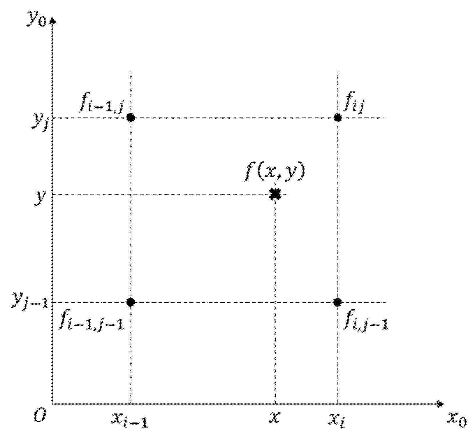
With reference to the Figure 3, the coefficient vector $\mathit{a}$ is evaluated solving the linear system (19) by imposing that the function $f$ must be equal to its value on the surrounding points $\left(i-1,j-1\right)$, $\left(i-1,j\right)$, $\left(i,j-1\right)$ and $\left(i,j\right)$ and the same is done for its partial derivatives along the $x$ direction, $f_x$, and the $y$ one, $f_y$.

$$\begin{array}{c}\{\begin{array}{l}{\mathit{a}}^T\mathit{\phi }\left(x_{i-1},y_{j-1}\right)=f_{i-1,j-1} \\ {\mathit{a}}^T\mathit{\phi }\left(x_{i-1},y_j\right)=f_{i-1,j} \\ {\mathit{a}}^T\mathit{\phi }\left(x_i,y_{j-1}\right)=f_{i,j-1}\\ {\mathit{a}}^T\mathit{\phi }\left(x_i,y_j\right)=f_{ij}\\ {\mathit{a}}^T{\mathit{\phi }}_x\left(x_{i-1},y_{j-1}\right)=f_{x_{i-1,j-1}}\\ {\mathit{a}}^T{\mathit{\phi }}_x\left(x_{i-1},y_j\right)=f_{x_{i-1,j}}\\ {\mathit{a}}^T{\mathit{\phi }}_x\left(x_i,y_{j-1}\right)=f_{x_{i,j-1}}\\ {\mathit{a}}^T{\mathit{\phi }}_x\left(x_i,y_j\right)=f_{x_{ij}}\\ {\mathit{a}}^T{\mathit{\phi }}_y\left(x_{i-1},y_{j-1}\right)=f_{y_{i-1,j-1}}\\ {\mathit{a}}^T{\mathit{\phi }}_y\left(x_{i-1},y_j\right)=f_{y_{i-1,j}}\\ {\mathit{a}}^T{\mathit{\phi }}_y\left(x_i,y_{j-1}\right)=f_{y_{i,j-1}}\\ {\mathit{a}}^T{\mathit{\phi }}_y\left(x_i,y_j\right)=f_{y_{ij}}\end{array}\begin{array}{c}\to \end{array}\begin{array}{c}\mathit{A}\mathit{a}=\mathit{b}\end{array}\end{array}$$

(19)

The vector $\mathit{b}$ is composed of the value of $f$ and its partial derivative along the two directions on the surroundings points—writing the partial derivatives with the central finite difference, the vector $\mathit{b}$ can be expressed as a function of the vector ${\mathit{f}}_s$ through a matrix $\mathit{M}$ defined in (20).

$$\begin{array}{c}\begin{array}{c}{\mathit{f}}_s={\left[\begin{array}{ccc}\begin{array}{cc}\begin{array}{cc}{f}_{i-1,j-2}& f_{i,j-2}\end{array}& \begin{array}{cc}{f}_{i-2,j-1}& f_{i-2,j}\end{array}\end{array}& \begin{array}{cc}\begin{array}{cc}{f}_{i-1,j-1}& f_{i-1,j}\end{array}& \begin{array}{cc}{f}_{i,j-1}& f_{ij}\end{array}\end{array}& \begin{array}{cc}\begin{array}{cc}{f}_{i-1,j+1}& f_{i,j+1}\end{array}& \begin{array}{cc}{f}_{i+1,j-1}& f_{i+1,j}\end{array}\end{array}\end{array}\right]}^T\\ \mathit{b}=\mathit{M}{\mathit{f}}_s\end{array}\end{array}$$

(20)

Since every point on the second grid can be calculated by the knowledge of the vector ${\mathit{f}}_s$, through the definition of a matrix ${\mathit{J}}_{01,s}$, then all the $f$ values on the second grid, included in the vector ${\mathit{f}}_1$, can be calculated through the assembled cubic interpolation matrix ${\mathit{J}}_{01}$ multiplied by the $f$ vector values on the starting grid, ${\mathit{f}}_0$, in (21).

$$\begin{array}{c}f\left(x,y\right)=\left({\mathit{\phi }}^T{\mathit{A}}^{-1}\mathit{M}\right){\mathit{f}}_s={\mathit{J}}_{01,s}{\mathit{f}}_s \to {\mathit{f}}_1={\mathit{J}}_{01}{\mathit{f}}_0\end{array}$$

(21)

In order to apply the Equation (21) to the grids belonging, respectively, to the inner surface of the acetabular cup, $\left\{{\theta }_c,{\phi }_c\right\}$, and to the outer surface of the femoral head, $\left\{{\theta }_h,{\phi }_h\right\}$, the position of the points defined in the grid of arrival has to be rotated in the reference frame of the starting grid because of the hip relative motion. With reference to the Figure 4 and denoting with ${\mathit{R}}_x$, ${\mathit{R}}_y$ and ${\mathit{R}}_z$ the rotation matrices around the cartesian axes, the global rotation between the two grids is composed of three transformations:

• Both for the acetabular cup and for the femoral head, the reference frame used in the finite element discretization was rotated by the inclination angle ${\alpha }_{in}$ and the anteversion angle ${\beta }_{av}$ with respect to the anatomical reference frame (Antero/Posterior AP, Proximo/Distal PD and Medio/Lateral ML) through a rotation matrix ${\mathit{R}}_g$ defined in (22) [3]; and

  $$\begin{array}{c}{\mathit{R}}_g={\mathit{R}}_z\left(\frac{\pi }{2}-{\beta }_{av}\right){\mathit{R}}_x\left(-{\alpha }_{in}\right)\end{array}$$

  (22)
• The head anatomical reference frame is rotated with respect to the cup one by the Flexion/Extension angle ${\theta }_{FE}$, the Adduction/Abduction angle ${\theta }_{AA}$ and the Internal/External Rotation angle ${\theta }_{IER}$ through the rotation matrix ${\mathit{R}}_{hip}$ defined in (23) [3].

  $$\begin{array}{c}{\mathit{R}}_{hip}={\mathit{R}}_z\left({\theta }_{FE}\right){\mathit{R}}_x\left({\theta }_{AA}\right){\mathit{R}}_y\left({\theta }_{IER}\right)\end{array}$$

  (23)

Then, the cup radial unit vector defined in the $x_c{y}_c{z}_c$ reference frame, ${\widehat{\mathit{r}}}_c$, can be written in the $x_h{y}_h{z}_h$ reference frame as ${\widehat{\mathit{r}}}_c^{\left(h\right)}$ in (24), together with the head radial unit vector ${\widehat{\mathit{r}}}_h$ rotated in the cup reference frame as ${\widehat{\mathit{r}}}_h^{\left(c\right)}$.

$$\begin{array}{c}\begin{array}{c}\widehat{\mathit{r}}={\left[\begin{array}{ccc}\sin \theta \cos \phi & \sin \theta \sin \phi & \cos \theta \end{array}\right]}^T\\ \begin{array}{cc}{\widehat{\mathit{r}}}_c^{\left(h\right)}={\mathit{R}}_g^T{\mathit{R}}_{hip}^T{\mathit{R}}_g{\widehat{\mathit{r}}}_c& {\widehat{\mathit{r}}}_h^{\left(c\right)}={\mathit{R}}_g^T{\mathit{R}}_{hip}{R}_g{\widehat{\mathit{r}}}_h\end{array}\end{array}\end{array}$$

(24)

Since the radial unit vector $\widehat{\mathit{r}}$ depends only on the spherical angles $\theta$ and $\phi$, the points of the cup grid $\left\{{\theta }_c,{\phi }_c\right\}$ can be rotated in the head grid obtaining the points $\left\{{\theta }_c^{\left(h\right)},{\phi }_c^{\left(h\right)}\right\}$ and the points of the head grid $\left\{{\theta }_h,{\phi }_h\right\}$ can be rotated in the cup grid obtaining the points $\left\{{\theta }_h^{\left(c\right)},{\phi }_h^{\left(c\right)}\right\}$ by inverting $\widehat{\mathit{r}}$ in (24) as follows in (25).

$$\begin{array}{c}\begin{array}{cc}\theta =\arctan \left(\frac{\sqrt{{\widehat{r}}_1^2+{\widehat{r}}_2^2}}{{\widehat{r}}_3}\right)& \phi =\arctan \left(\frac{{\widehat{r}}_2}{{\widehat{r}}_1}\right)\end{array}\end{array}$$

(25)

Once the rotated grids are obtained, the cubic interpolation matrix that leads from the cup to the head ${\mathit{J}}_{ch}$ and the one that leads from the head to the cup ${\mathit{J}}_{hc}$ can be assembled. Generally, a lubrication model algorithm is referred to the cup grid, so the calculated cubic interpolation matrices can be used together with Equation (17) in order to evaluate in (26) the total deformation of both the surfaces $\mathit{\delta }$ due to the pressure $\mathit{p}$ acting on them in the cup grid reference frame.

$$\begin{array}{c}\{\begin{array}{l}{\mathit{\delta }}_c={\mathit{C}}_c{\mathit{p}}_c+{\mathit{n}}_c\\ {\mathit{\delta }}_h={\mathit{C}}_h{\mathit{p}}_h+{\mathit{n}}_h\\ \mathit{\delta }={\mathit{\delta }}_c+{\mathit{J}}_{hc}{\mathit{\delta }}_h\\ {\mathit{p}}_c=\mathit{p}\\ {\mathit{p}}_h={\mathit{J}}_{ch}{\mathit{p}}_c\end{array} \to \mathit{\delta }=\left({\mathit{C}}_c+{\mathit{J}}_{hc}{\mathit{C}}_h{\mathit{J}}_{ch}\right)\mathit{p}+\left({\mathit{n}}_c+{\mathit{J}}_{hc}{\mathit{n}}_h\right)\end{array}$$

(26)

In Equation (27), the final form of the influence matrix $\mathit{C}$ and of the boundary conditions vector $\mathit{n}$ constituting the definitive deformation model is highlighted.

$$\begin{array}{c}\{\begin{array}{l}\mathit{C}={\mathit{C}}_c+{\mathit{J}}_{hc}{\mathit{C}}_h{\mathit{J}}_{ch}\\ \mathit{n}={\mathit{n}}_c+{\mathit{J}}_{hc}{\mathit{n}}_h\end{array} \to \mathit{\delta }=\mathit{C}\mathit{p}+\mathit{n}\end{array}$$

(27)

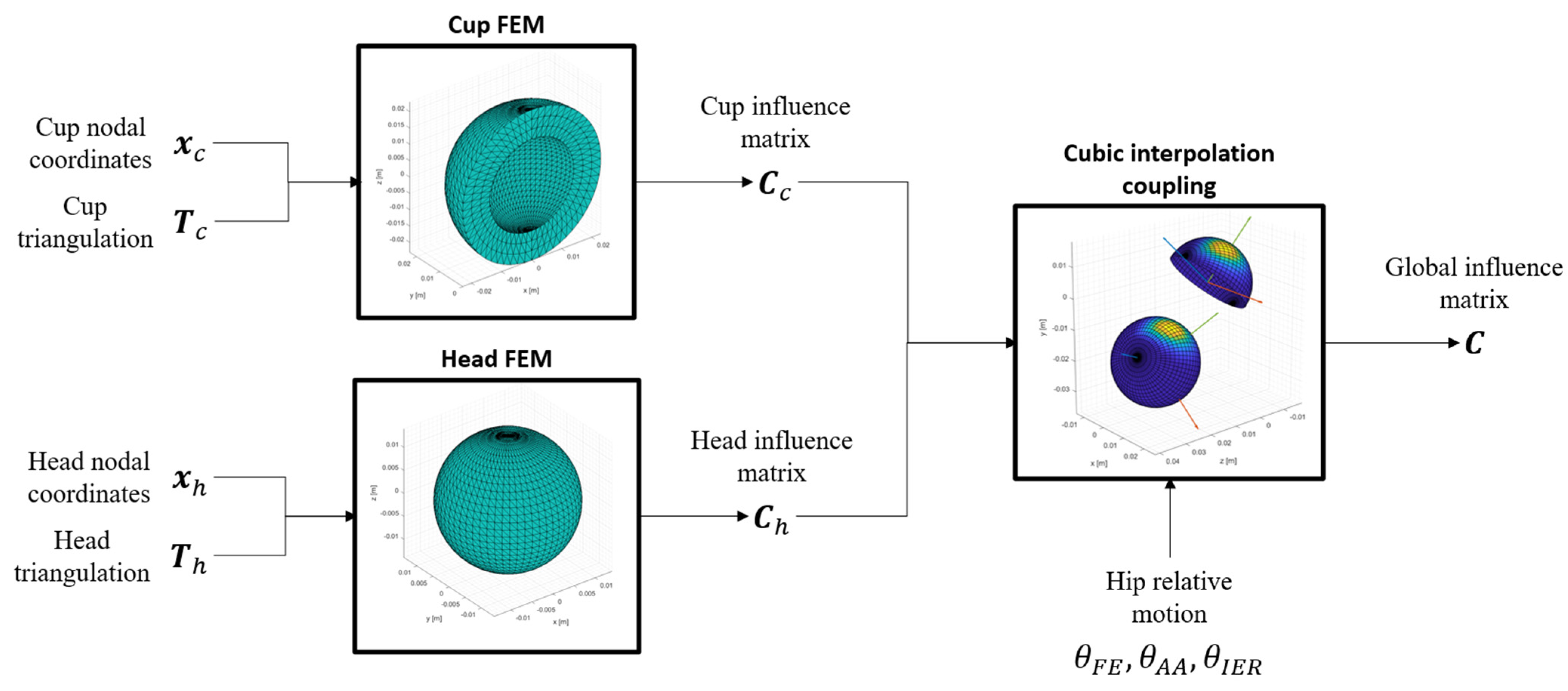
Finally, the whole deformation model logic is shown in the Figure 5 through block visualizations, in which the calculation of the boundary conditions vector $\mathit{n}$ is not considered because of the reasons explained in the Section 2.2.

3. Results and Discussion

3.1. Validation

In order to validate Equation (17), two simulations (one for the acetabular cup and one for the femoral head) were performed in the Matlab environment (Matlab R2020b, Mathworks, Natick, Massachusetts, USA). Their results were compared with the ones computed by the software Ansys Mechanical (Ansys 2020 R2, Canonsburg, Pennsylvania, USA) for the same inputs (pressure field, mechanical and geometrical properties) but for discretization performed with quadratic tetrahedral elements instead of the linear ones used in the proposed model. The second order quadratic tetrahedral finite elements used in Ansys allows us to work with coarser mesh with respect to the one used in Matlab; moreover, the Matlab mesh is strictly connected to the interface grid on the acetabular cup surface because it will be used successively in an elasto-hydrodynamic lubrication algorithm.

The input pressure fields, characteristics of elasto-hydrodynamic lubrication shapes [3], were used in the simulations with zero pressure on the domain boundaries, both for the cup simulation and for the head one, as follows in (28).

$$\begin{array}{c}{p}_c\left({\theta }_c,{\phi }_c\right)=\left(p_0{e}^{- \frac{{\left({\theta }_c-{\theta }_0\right)}^2+{\left({\phi }_c-{\phi }_0\right)}^2}{{\left({\alpha }_0\pi \right)}^2}}\right)\sin {\theta }_c\sin {\phi }_c\\ p_h\left({\theta }_h,{\phi }_h\right)=\{\begin{array}{ll}\left(p_0{e}^{- \frac{{\left({\theta }_h-{\theta }_0\right)}^2+{\left({\phi }_h-{\phi }_0\right)}^2}{{\left({\alpha }_0\pi \right)}^2}}\right)\sin {\theta }_h\sin {\phi }_h& \mathrm{if}0\le {\phi }_h\le \pi \\ 0& \mathrm{if}\pi <{\phi }_h\le 2\pi \end{array}\end{array}$$

(28)

The input parameters used in the calculations are listed in the

Table 1. Input parameters related to the comparative simulations.

Parameter	Value
Femoral head radius r	14 mm
Acetabular cup inner radius R	14.03 mm
Acetabular cup thickness H	9 mm
Femoral head fixed nodes angle ${\varphi }_0$	30°
Acetabular cup Young modulus $E_c$	1.1 GPa
Acetabular cup Poisson ratio ${\nu }_c$	0.42
Femoral head Young modulus $E_h$	245.9 GPa
Femoral head Poisson ratio ${\nu }_h$	0.24
Pressure gaussian peak $p_0$	107 Pa
Pressure gaussian θ-translation ${\theta }_0$	2π/3 rad
Pressure gaussian φ-translation ${\phi }_0$	π/3 rad
Pressure gaussian dimensionless width ${\alpha }_0$	0.2

. Regarding the mechanical properties, they are referred to a plastic acetabular cup (Polyethylene) and a ceramic femoral head (Alumina 88%).

The pressure fields of Equation (28) were described in Matlab code—in order to apply them within the Ansys simulations, the mesh generated by Ansys was imported in the Matlab algorithm, and the pressure field was interpolated through a cubic interpolation matrix on the Ansys mesh nodes and, after, it was imported back in the Ansys model as External Data. In Figure 6, the Ansys meshes related to the acetabular cup and the femoral head together with the surface pressure fields are shown.

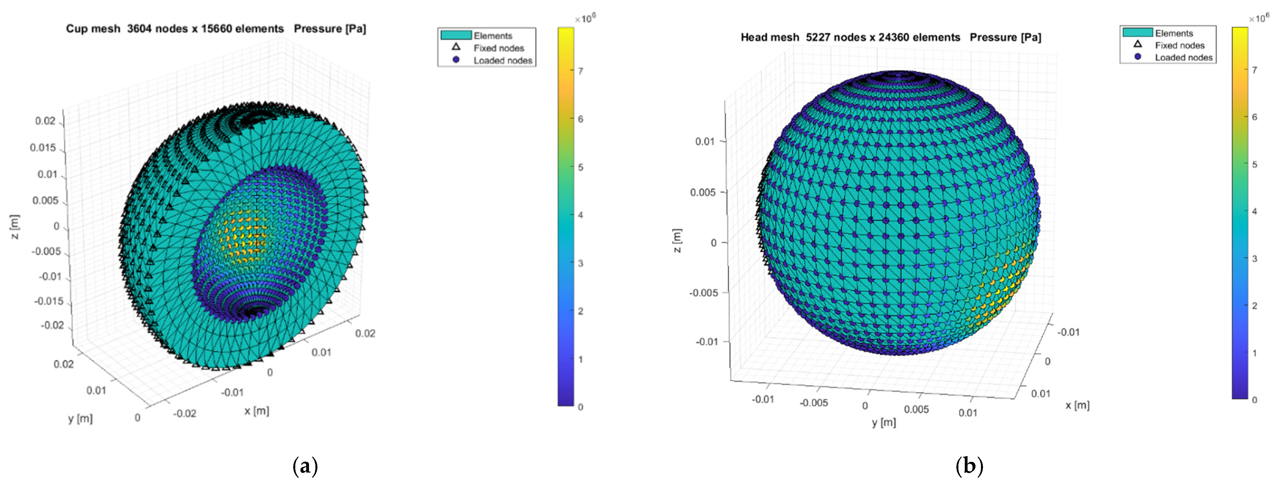
The same information shown in Figure 6 is reported in Figure 7 but related to the Matlab model.

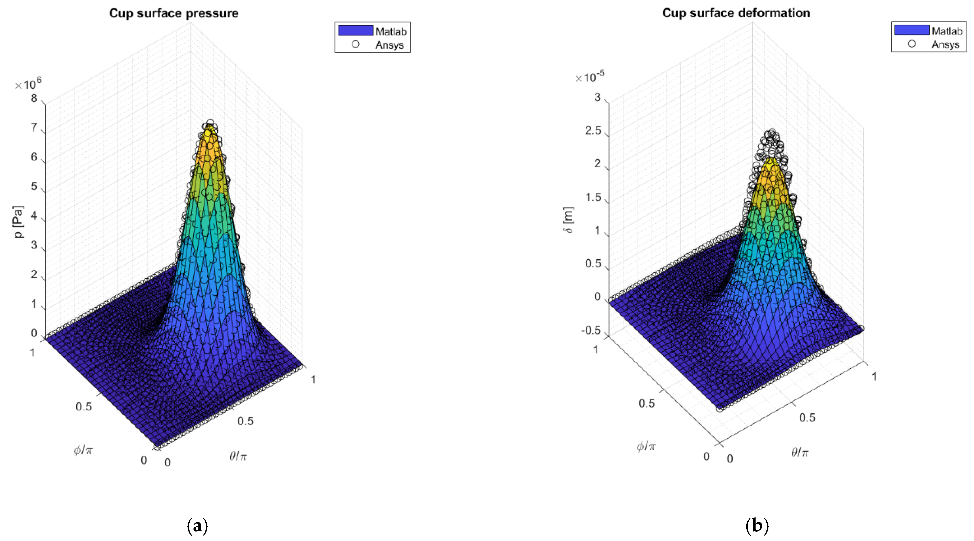
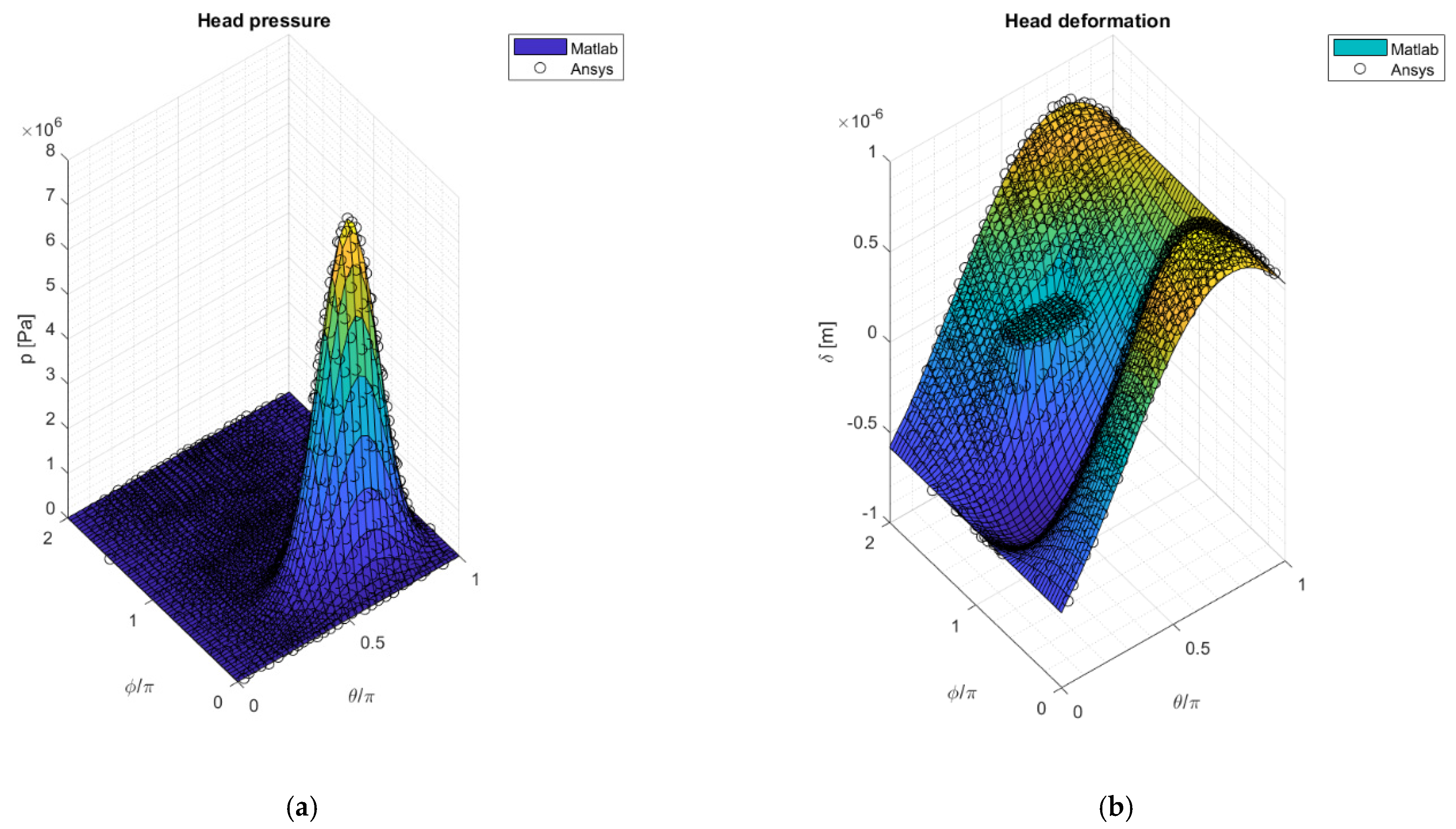
In order to compare the surfaces’ deformation, the Ansys solution results are evaluated in terms of directional deformations along the cartesian axes; then, they are projected along the radial direction so that the normal surface deformation is obtained. In Figure 8, the input surface pressure and the output surface deformation of the acetabular cup are shown over the cup grid, both for the Matlab simulation and for the Ansys one. The results show a general satisfactory agreement between the two software in terms of deformation shapes, peak coordinates and magnitude even if a slight underestimation is detected close to deformation peak—this is probably due to different finite element used in Ansys (quadratic tetrahedra) and the adopted choice to distribute uniformly the nodal pressures over the loaded face of a tetrahedron though their arithmetic average. However, also the choice of using of the linear tetrahedra allows us to perform the influence matrix assembly easily and this results in unappreciable underestimation.

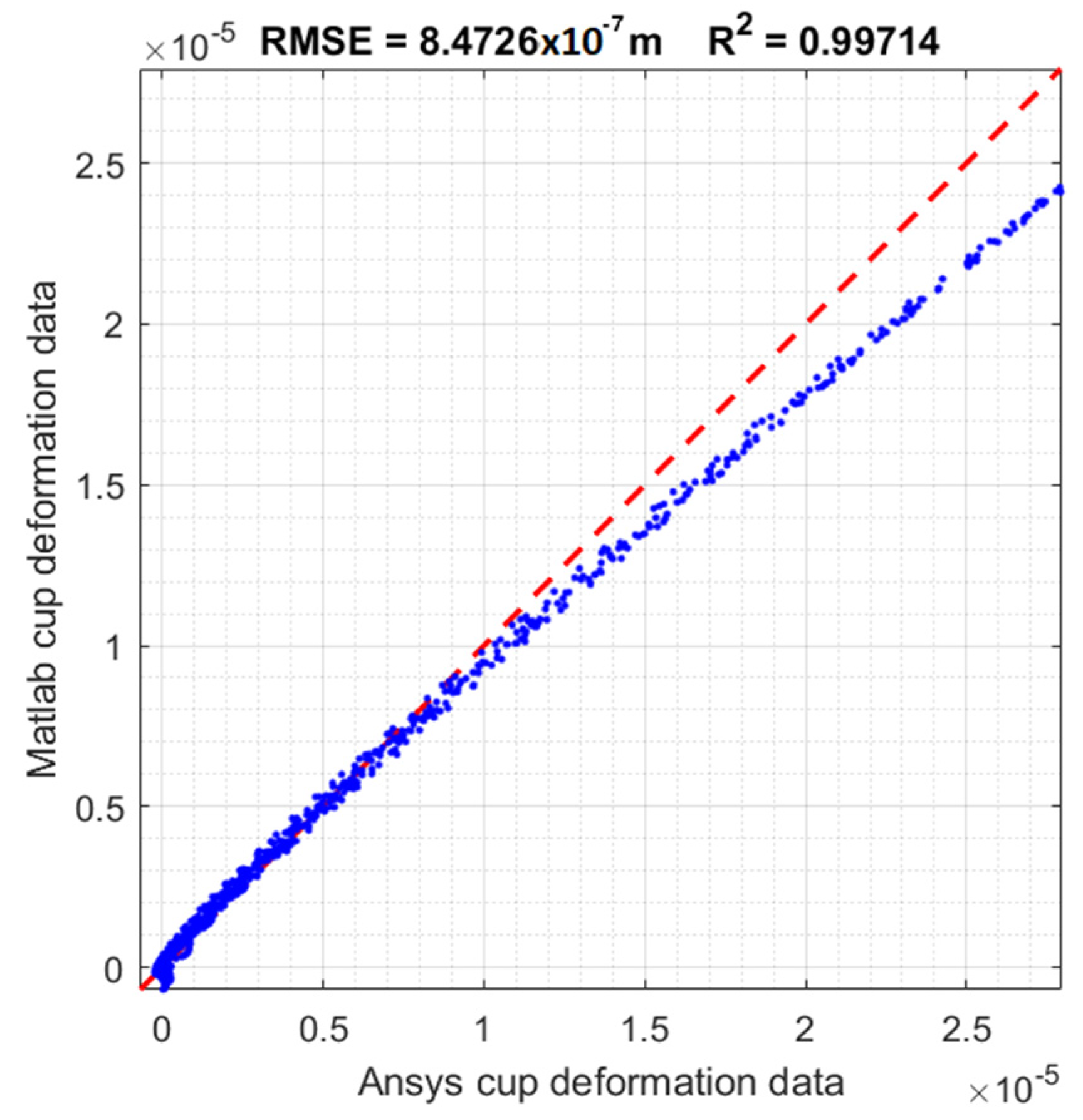
In order to validate the model, the Root Mean Square Error (RMSE) and the squared correlation coefficient $R^2$ between the deformation results are calculated and the related data are plotted against each other in the Figure 9—the plot confirms the underestimation close to the highest values of the deformation but provides good values of the RMSE and the $R^2$, respectively, $8.47 \times {10}^{-7} \mathrm{m}$ and $0.99714$.

Then, the same comparison was performed within the femoral head simulation. In Figure 10, the head surface pressure and deformation over the head grid, both in Matlab and in Ansys, are shown. With respect to the acetabular cup case, the results were even more satisfactory—a dominant underestimation or overestimation is not appreciable and the discontinuities generated by the imposed boundary conditions, in terms of null displacement in correspondence of the femoral head fixation, do not result in output instabilities.

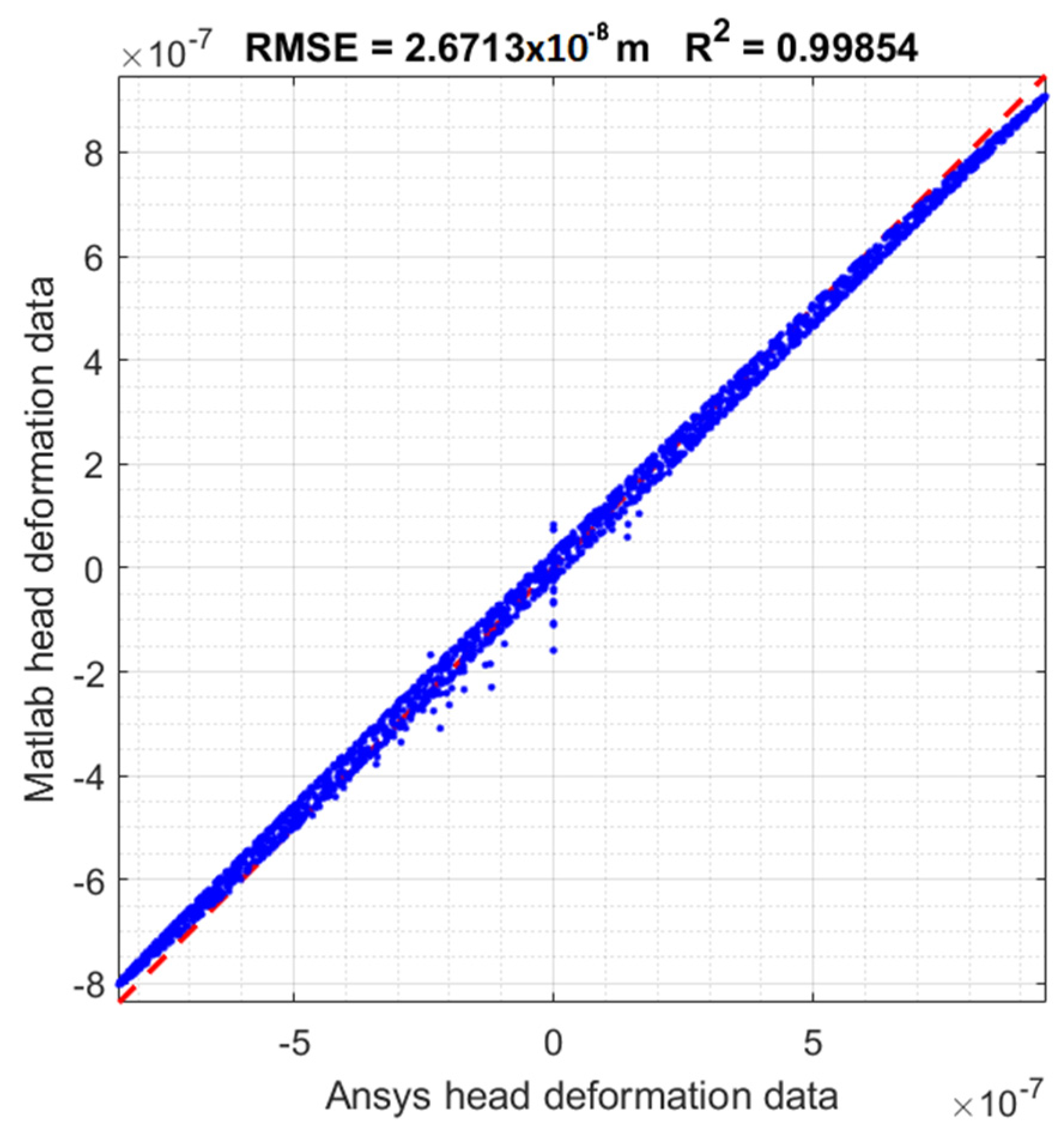
In Figure 11, the Matlab deformation data are plotted against the Ansys one for the femoral head simulation, showing two slight deviations—an overestimation for the lowest deformation values and an underestimation for the highest ones. In this case the RMSE and the $R^2$ obtained are, respectively, $2.67 \times {10}^{-8} \mathrm{m}$ and $0.99854$.

It is interesting to notice that, despite the fact that the influence matrix $\mathit{C}$ is referred to the interface between the acetabular cup and the femoral head (in fact it relates the surface deformation $\mathit{\delta }$ to the surface pressure $\mathit{p}$), it is built by rearranging the global stiffness matrix $\mathit{K}$ and the nodal displacement $\mathit{q}$ and force $\Phi$ vectors associated with the two analysed bodies according to the classical Finite Element theory, so other quantities referring instead to the bodies’ bulk continuum are evaluable, such as for example the Von Mises equivalent stress and the strain energy.

Then, these quantities can be calculated also with the Matlab code, so they can be compared. In Figure 12 the above quantities are shown for the cup simulation in Ansys.

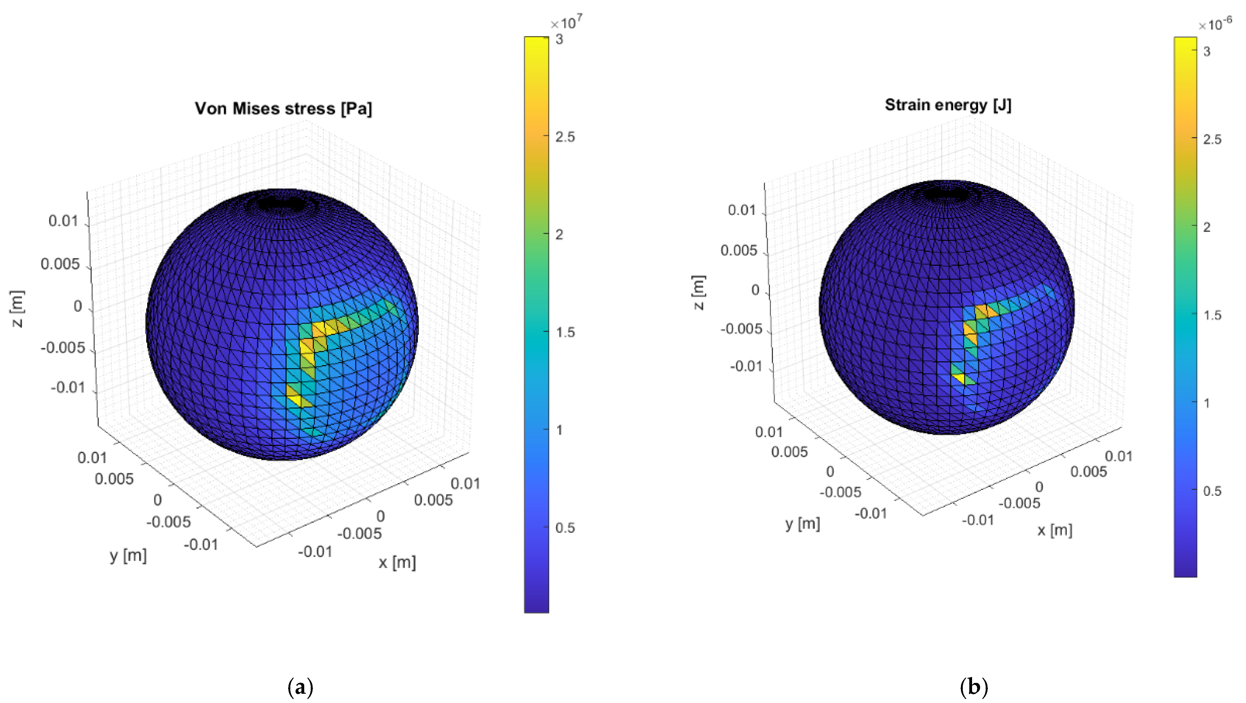
The same quantities obtained by the Matlab code are shown in the Figure 13—the comparison is satisfactory in terms of magnitude order and shapes matching.

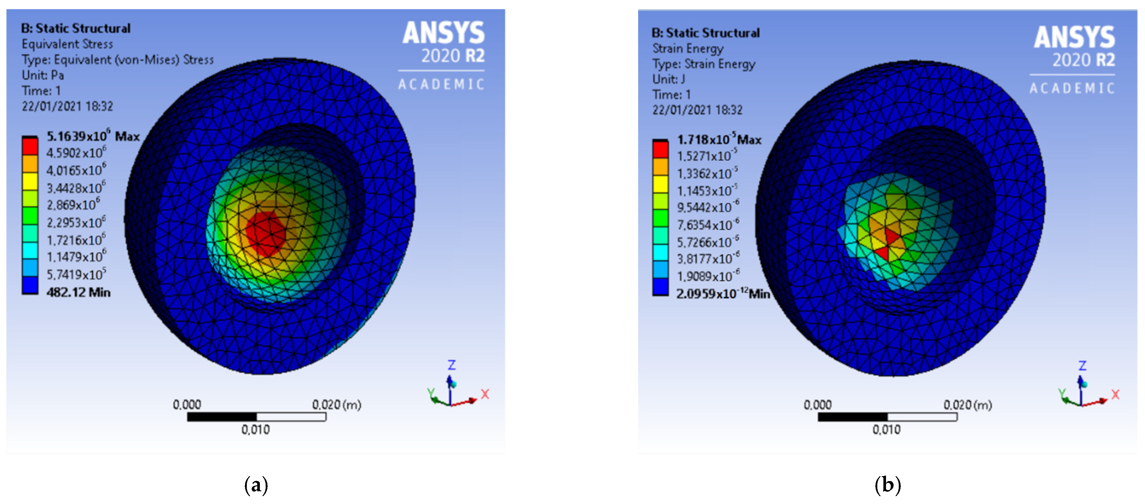
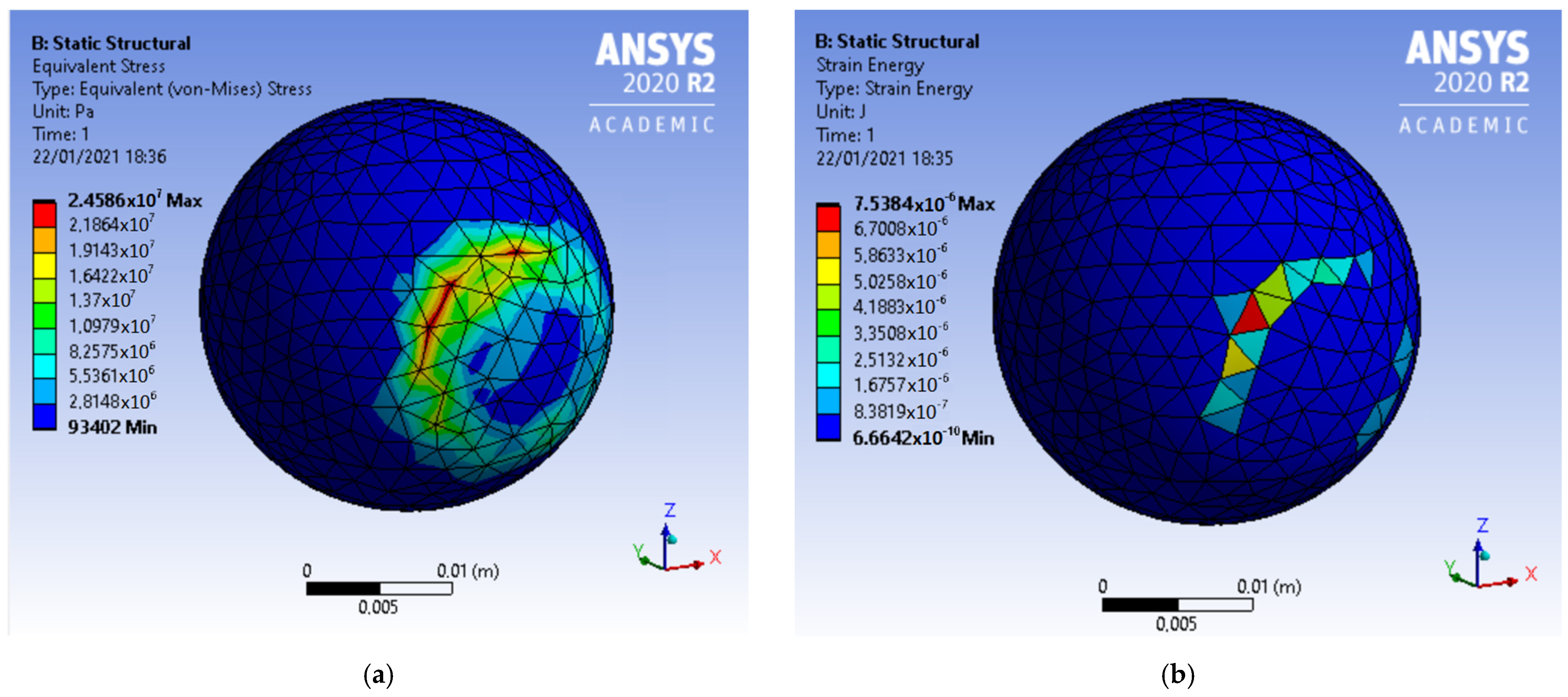
The same comparison is performed for the femoral head case. In Figure 14, the Von Mises stress and the strain energy in the Ansys environment are shown.

Then, Figure 15 reports the same outputs obtained by Matlab code. In this case, the comparison provides less satisfactory agreements regarding the strain energy—this could be due to the particular boundary conditions imposed on the fixed nodes, which lead to remarkable discontinuities around that zone, as confirmed by Figure 10 and Figure 14.

3.2. Implementation of the Deformation Model in an EHL Lubrication Algorithm

In the context of an elasto-hydrodynamic lubrication algorithm, the proposed deformation model accomplishes the task of calculating the lubricating fluid gap contribution due to the surfaces’ deformation considering also the hip relative motion. In particular, according to Equation (29) the fluid gap field $h$ is composed of the geometrical gap, dependent on the radial clearance $c$ and the dimensionless eccentricity vector $\mathit{n}$, added to the surfaces’ deformation $\delta$ [3,4].

$$\begin{array}{c}h\left(\theta ,\phi \right)=c\left(1-{\mathit{n}}^T\widehat{\mathit{r}}\left(\theta ,\phi \right)\right)+\delta \left(p\left(\theta ,\phi \right)\right)\end{array}$$

(29)

In order to give an example in which the cubic interpolation matrices are used, the surfaces’ deformation over the cup grid is calculated for the same prosthesis characterized by the data listed in the Table 1, but with different parameters related to the gaussian input surface pressure and with a configuration defined by a relative position between the acetabular cup and femoral head deriving from a previously algorithm developed in [3,4].

The new data are listed in the

Table 2. Input parameters related to the simulation with relative rotations between the acetabular cup and the femoral head.

Parameter	Value
Pressure gaussian peak $p_0$	107 Pa
Pressure gaussian θ-translation ${\theta }_0$	π/4 rad
Pressure Gaussian φ-translation ${\phi }_0$	π/4 rad
Pressure gaussian dimensionless width ${\alpha }_0$	0.2
Anteversion angle ${\beta }_{av}$	90°
Inclination angle ${\alpha }_{in}$	45°
Flexion/Extension angle ${\theta }_{FE}$	−40°
Adduction/Abduction angle ${\theta }_{AA}$	10°
Internal/External Rotation angle ${\theta }_{IER}$	2°

.

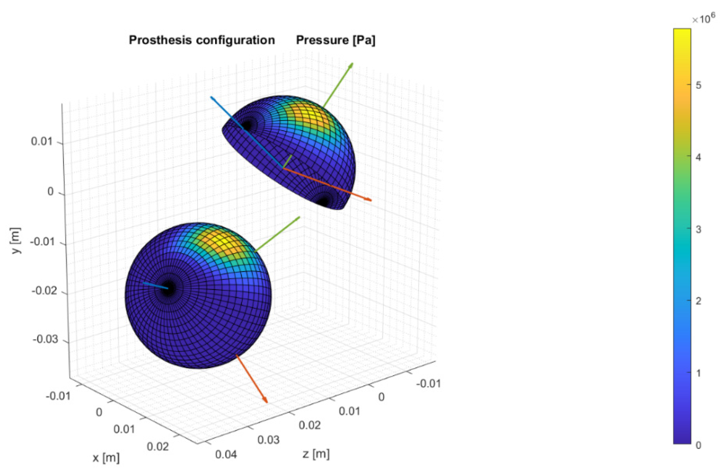
In Figure 16, the prosthesis configuration is shown in the anatomical reference frame of the cup in terms of surfaces’ grids, together with the fluid pressure acting on the two surfaces of the joint and the local reference frames with red $x$-axis, green $y$-axis and blue $z$-axis.

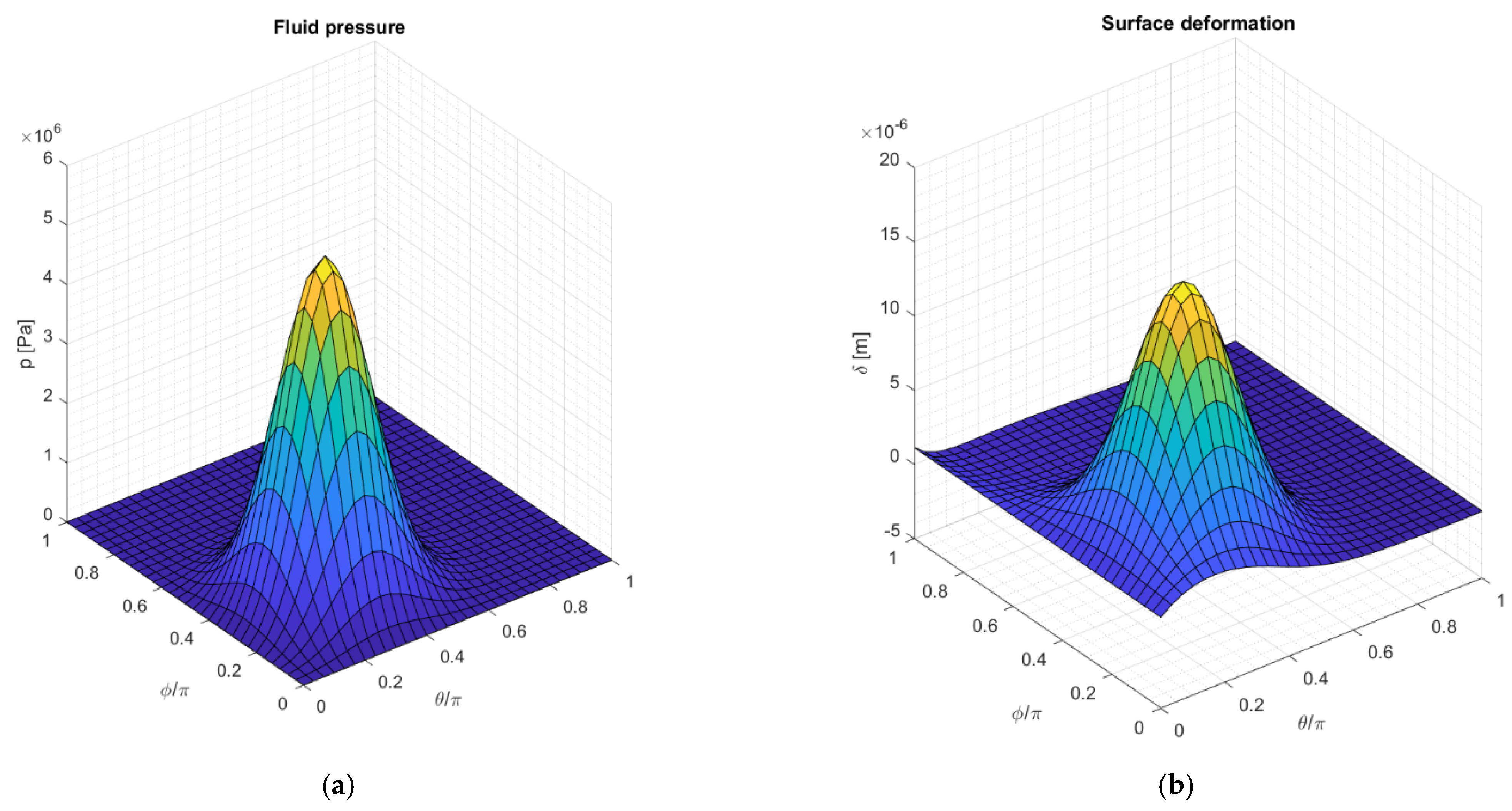
Once the cubic interpolation matrices are built with Equation (21) while the influence matrix and the boundary conditions vector are assembled through Equation (27), the resultant surfaces’ deformation is calculated and shown in Figure 17 together with the surface pressure.

4. Conclusions

In this work, an accurate model for the calculation of the total hip replacement surfaces deformation was proposed with the aim to merge it in EHL lubrication algorithms. The computer code was based on the finite element theory by discretizing the acetabular cup and the femoral head bodies in linear tetrahedra; the elements located on the loaded surfaces are subjected to nodal forces due to the lubricating surface pressure, evaluated by the virtual work principle. The two discretizations of the prosthesis were coupled through a cubic interpolation matrix which connects the two surfaces grids and takes into account the relative motion between the acetabular cup and the femoral head. The model was developed in order to define a global influence matrix and a boundary conditions vector, so that it can be run in the same computational context of an elasto-hydrodynamic lubrication algorithm taking advantage of its accuracy. In order to validate the proposed code, two simulations were conducted and compared with the results elaborated by the software Ansys working with quadratic tetrahedra for the same problem—in particular the surfaces’ deformation of a prosthesis made of a polyethylene acetabular cup and Alumina 88% femoral head was evaluated as a consequence of a surface pressure field modelled with a modified gaussian shape. The comparison provided a satisfactory agreement in terms of surfaces deformation, in particular recording a root mean squared error RMSE and a squared correlation coefficient $R^2$ equal to, respectively,$8.47\times {10}^{-7} \mathrm{m}$ and $0.99714$ for the acetabular cup simulation and equal to $2.67\times {10}^{-8} \mathrm{m}$ and $0.99854$ for the femoral head one. Then, the outputs regarding the Von Mises stress and the strain energy were compared resulting in a good matching in terms of magnitude order and shapes.

A third simulation was conducted to evaluate the prosthesis deformation due to a similar pressure field but with an implant configuration which considers a relative rotation between the surfaces due to the hip motion, in order to show the simplicity of implementation of the deformation model in an elasto-hydrodynamic lubrication code.

Finally, the proposed model showed quantitative and qualitative reliability, so that several insights can be conducted and the related future perspectives could regard:

• The implementation of a routine which elaborates the contact pressure in domain zones characterized by nodes overlapping, in order to consider the model functionality within a mixed elasto-hydrodynamic lubrication algorithm;
• The adaptation of the finite element model to consider viscoelastic materials, adding deformation contributions which depend on the time history of the pressure field through a viscosity matrix;
• The usage of the model for other types of joint replacements such as knee, ankle, shoulders, etc.

References

1. Fisher, J.; Dowson, D. Tribology of Total Artificial Joints. Proc. Inst. Mech. Eng. Part H J. Eng. Med. 1991, 205, 73–79. [Google Scholar] [CrossRef]
2. Ruggiero, A.; Sicilia, A. Lubrication modeling and wear calculation in artificial hip joint during the gait. Tribol. Int. 2020, 142, 105993. [Google Scholar] [CrossRef]
3. Ruggiero, A.; Sicilia, A. A Mixed Elasto-Hydrodynamic Lubrication Model for Wear Calculation in Artificial Hip Joints. Lubricants 2020, 8, 72. [Google Scholar] [CrossRef]
4. Ruggiero, A.; Sicilia, A.; Affatato, S. In silico total hip replacement wear testing in the framework of ISO 14242-3 accounting for mixed elasto-hydrodynamic lubrication effects. Wear 2020, 460, 203420. [Google Scholar] [CrossRef]
5. Mattei, L.; Di Puccio, F.; Piccigallo, B.; Ciulli, E. Lubrication and wear modelling of artificial hip joints: A review. Tribol. Int. 2011, 44, 532–549. [Google Scholar] [CrossRef]
6. Gleghorn, J.P.; Bonassar, L.J. Lubrication mode analysis of articular cartilage using Stribeck surfaces. J. Biomech. 2008, 41, 1910–1918. [Google Scholar] [CrossRef]
7. Scholes, S.C.; Unsworth, A. Comparison of friction and lubrication of different hip prostheses. Proc. Inst. Mech. Eng. Part H J. Eng. Med. 2000, 214, 49–57. [Google Scholar] [CrossRef]
8. Ruggiero, A.; Merola, M.; Affatato, S. Finite element simulations of hard-on-soft hip joint prosthesis accounting for dynamic loads calculated from a musculoskeletal model during walking. Materials 2018, 11, 574. [Google Scholar] [CrossRef] [Green Version]
9. Affatato, S.; Ruggiero, A. A Perspective on Biotribology in Arthroplasty: From In Vitro toward the Accurate In Silico Wear Prediction. Appl. Sci. 2020, 10, 6312. [Google Scholar] [CrossRef]
10. Jalali-Vahid, D.; Jagatia, M.; Jin, Z.M.; Dowson, D. Prediction of lubricating film thickness in a ball-in-socket model with a soft lining representing human natural and artificial hip joints. Proc. Inst. Mech. Eng. Part J J. Eng. Tribol. 2001, 215, 363–372. [Google Scholar] [CrossRef]
11. Jalali-Vahid, D.; Jin, Z.M.; Dowson, D. Elastohydrodynamic lubrication analysis of hip implants with ultra high molecular weight polyethylene cups under transient conditions. Proc. Inst. Mech. Eng. Part C J. Mech. Eng. Sci. 2003, 217, 767–777. [Google Scholar] [CrossRef]
12. Jalali-Vahid, D.; Jagatia, M.; Jin, Z.; Dowson, D. Prediction of lubricating film thickness in UHMWPE hip joint replace-ments. J. Biomech. 2001, 34, 261–266. [Google Scholar] [CrossRef]
13. Jalali-Vahid, D.; Jin, Z.M. Transient elastohydrodynamic lubrication analysis of ultra-high molecular weight polyethylene hip joint replacements. Proc. Inst. Mech. Eng. Part C J. Mech. Eng. Sci. 2001, 216, 409–420. [Google Scholar] [CrossRef]
14. Fregly, B.J.; Bei, Y.; Sylvester, M.E. Experimental evaluation of an elastic foundation model to predict contact pressures in knee replacements. J. Biomech. 2003, 36, 1659–1668. [Google Scholar] [CrossRef]
15. Halloran, J.P.; Easley, S.K.; Petrella, A.J.; Rullkoetter, P.J. Comparison of deformable and elastic foundation finite element simulations for predicting knee replacement mechanics. J. Biomech. Eng. 2005, 127, 813–818. [Google Scholar] [CrossRef]
16. Askari, E.; Andersen, M.S. A closed-form formulation for the conformal articulation of metal-on-polyethylene hip prostheses: Contact mechanics and sliding distance. Proc. Inst. Mech. Eng. Part H J. Eng. Med. 2018, 232, 1196–1208. [Google Scholar] [CrossRef] [Green Version]
17. Pérez-González, A.; Fenollosa-Esteve, C.; Sancho-Bru, J.L.; Sánchez-Marín, F.T.; Vergara, M.; Rodríguez-Cervantes, P.J. A modified elastic foundation contact model for application in 3D models of the prosthetic knee. Med. Eng. Phys. 2008, 30, 387–398. [Google Scholar] [CrossRef]
18. Mukras, S.M.; Kim, N.H.; Schmitz, T.L.; Sawyer, W.G. Evaluation of contact force and elastic foundation models for wear analysis of multibody systems. In Proceedings of the International Design Engineering Technical Conferences and Computers and Information in Engineering Conference, Montreal, QC, Canada, 15–18 August 2010; Volume 44106, pp. 1565–1577. [Google Scholar]
19. Srivastava, G.; Christian, N.; Higgs, C.F., III. A predictive framework of the tribological impact of physical activities on metal-on-plastic hip implants. Biotribology 2021, 25, 100156. [Google Scholar] [CrossRef]
20. Wang, F.; Jin, Z. Prediction of elastic deformation of acetabular cups and femoral heads for lubrication analysis of artificial hip joints. Proc. Inst. Mech. Eng. Part J J. Eng. Tribol. 2004, 218, 201–209. [Google Scholar] [CrossRef]
21. Evans, H.P.; Hughes, T.G. Evaluation of deflection in semi-infinite bodies by a differential method. Proc. Inst. Mech. Eng. Part C J. Mech. Eng. Sci. 2000, 214, 563–584. [Google Scholar] [CrossRef]
22. Gao, L.; Dowson, D.; Hewson, R.W. Predictive wear modeling of the articulating metal-on-metal hip replacements. J. Biomed. Mater. Res. Part B Appl. Biomater. 2015, 105, 497–506. [Google Scholar] [CrossRef]
23. Jagatia, M.; Jin, Z. Elastohydrodynamic lubrication analysis of metal-on-metal hip prostheses under steady state entraining motion. Proc. Inst. Mech. Eng. Part H J. Eng. Med. 2001, 215, 531–541. [Google Scholar] [CrossRef]
Figure 1. Linear tetrahedron with I, J, K, and H nodes subjected to nodal pressures acting on the face IJK.
Lubricants 09 00041 g001
Figure 2. Acetabular cup (a) and femoral head (b) meshes in the related reference frames.
Lubricants 09 00041 g002
Figure 3. A 2D interpolation scheme with the points surrounding the desired evaluation.
Lubricants 09 00041 g003
Figure 4. Reference frames of the hip joint.
Lubricants 09 00041 g004
Figure 5. Deformation model blocks logic.
Lubricants 09 00041 g005
Figure 6. Ansys meshes and pressure loaded surfaces—acetabular cup (a) and femoral head (b).
Lubricants 09 00041 g006
Figure 7. Matlab meshes and pressure loaded surfaces—acetabular cup (a) and femoral head (b).
Lubricants 09 00041 g007
Figure 8. Acetabular cup surface pressure input in Matlab (surf) and Ansys (black circles) (a); Matlab deformation output (surf) and Ansys deformation output (black circles) related to the acetabular cup (b).
Lubricants 09 00041 g008
Figure 9. Matlab deformation results data against Ansys ones regarding the acetabular cup simulation.
Lubricants 09 00041 g009
Figure 10. Femoral head surface pressure input in Matlab (surf) and Ansys (black circles) (a); Matlab deformation output (surf) and Ansys deformation output (black circles) related to the femoral head (b).
Lubricants 09 00041 g010
Figure 11. Matlab deformation results data against Ansys ones regarding the femoral head simulation.
Lubricants 09 00041 g011
Figure 12. Von Mises stress (a) and strain energy (b) within the acetabular cup simulation in Ansys.
Lubricants 09 00041 g012
Figure 13. Von Mises stress (a) and strain energy (b) within the acetabular cup simulation in Matlab.
Lubricants 09 00041 g013
Figure 14. Von Mises stress (a) and strain energy (b) within the femoral head simulation in Ansys.
Lubricants 09 00041 g014
Figure 15. Von Mises stress (a) and strain energy (b) within the femoral head simulation in Matlab.
Lubricants 09 00041 g015
Figure 16. Prosthesis configuration due the chosen relative rotations.
Lubricants 09 00041 g016
Figure 17. Fluid pressure input (a) and total surface deformation results obtained (b).
Lubricants 09 00041 g017