Experimental and Numerical Investigation of Tire Tread Wear on Block Level


 and
and
Abstract
:1. Introduction
2. Materials and Methods
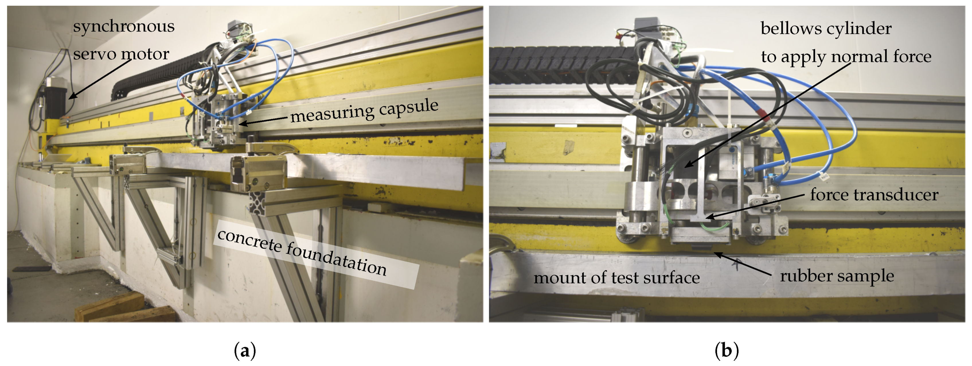
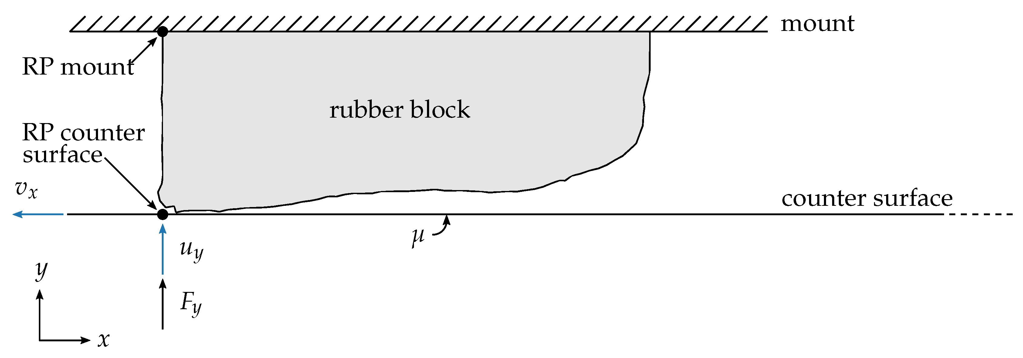
2.1. Experimental Setup
2.2. Test Procedure
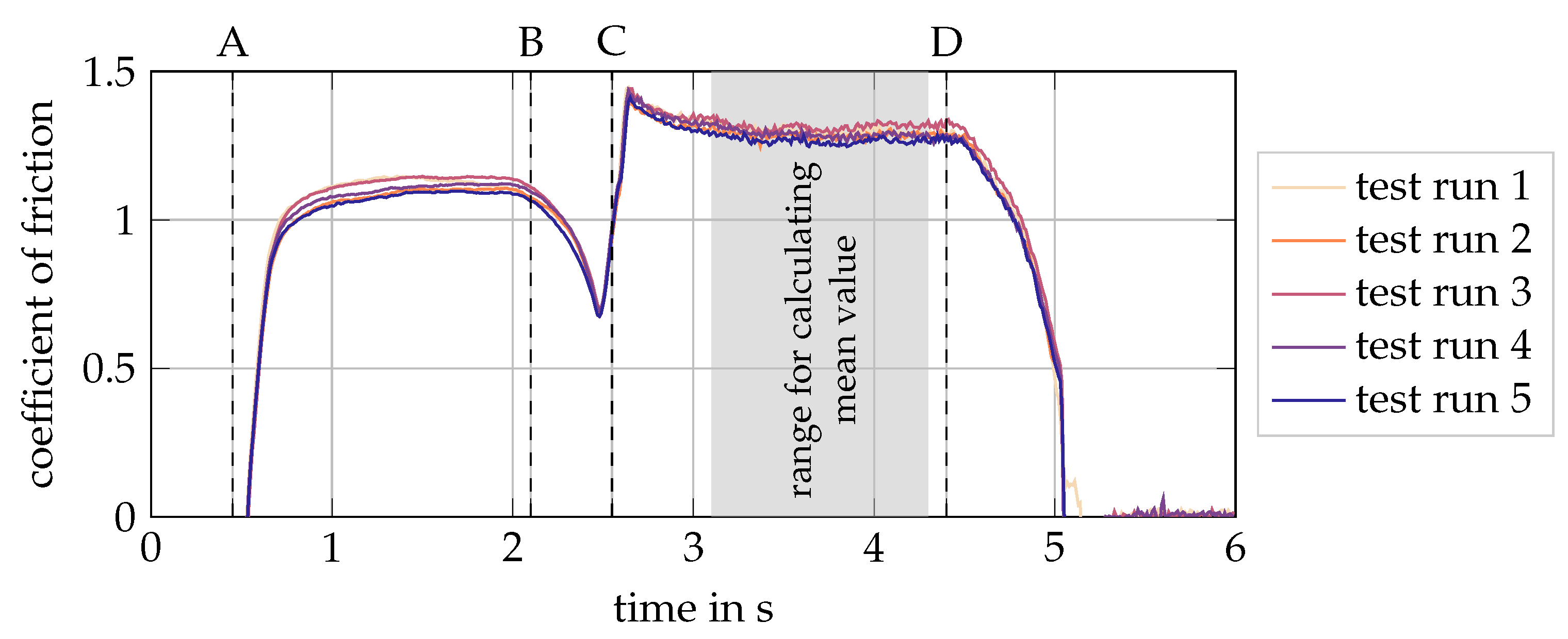
- A
- Sample is set down into contact with the aluminum sheet on track, with no relative motion until all vibrations are stopped. Normal force is applied via a pneumatic bellows cylinder. The resting time before start of motion is approximately . Then, acceleration with to the intended speed still on the aluminum track. The length of the aluminum track is large enough to ensure that the acceleration phase of the sample is finished before coming into contact with the abrasive test surface;
- B
- Leaving the aluminum sheet and coming into contact with the abrasive surface. Short phase of vertical dynamics because of the step down to the track with respective effects in signal of coefficient of friction;
- C
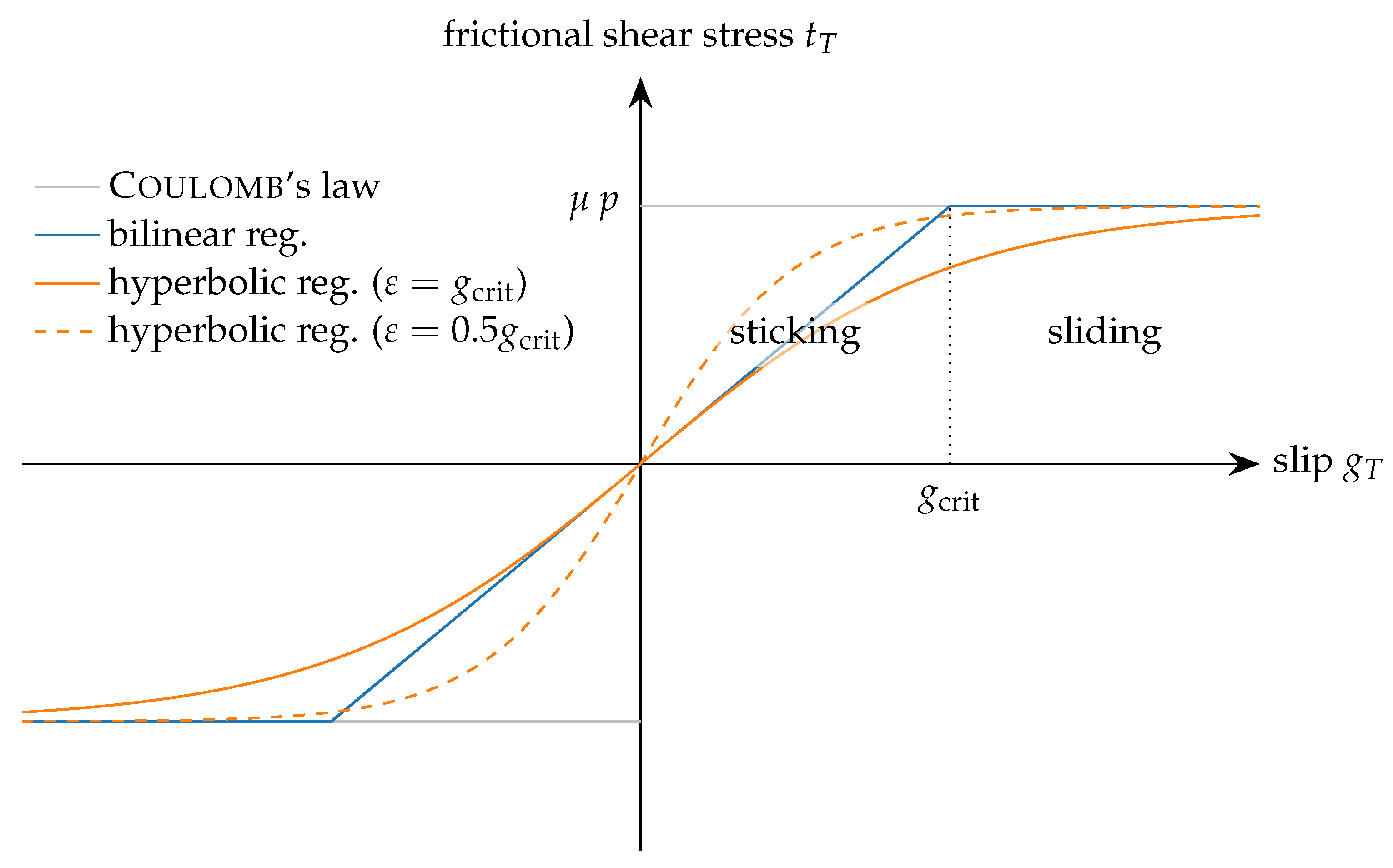
- Overcoming the static friction of the sample on the abrasive counter surface. For the transfer of results to rolling friction, assessment of the static friction coefficient is essential due to the large contribution of the sticking zone to the tangential forces in the tire footprint. Transitioning from sticking to sliding requires some time, in particular steady-state temperatures and block deflection have to be established. In this transition period, the coefficient of friction decreases slightly. The transition time lag constants are specific for the respective frictional contact and affected by materials, surface topographies, and potential third media in contact. Subsequently, a quasi-steady period of sliding friction occurs with a constant level of coefficient of friction, which is evaluated as the steady-state coefficient of friction;
- D
- At the end of the test track, the sample is decelerated and leaves the contact.
2.3. Material Model for Rubber
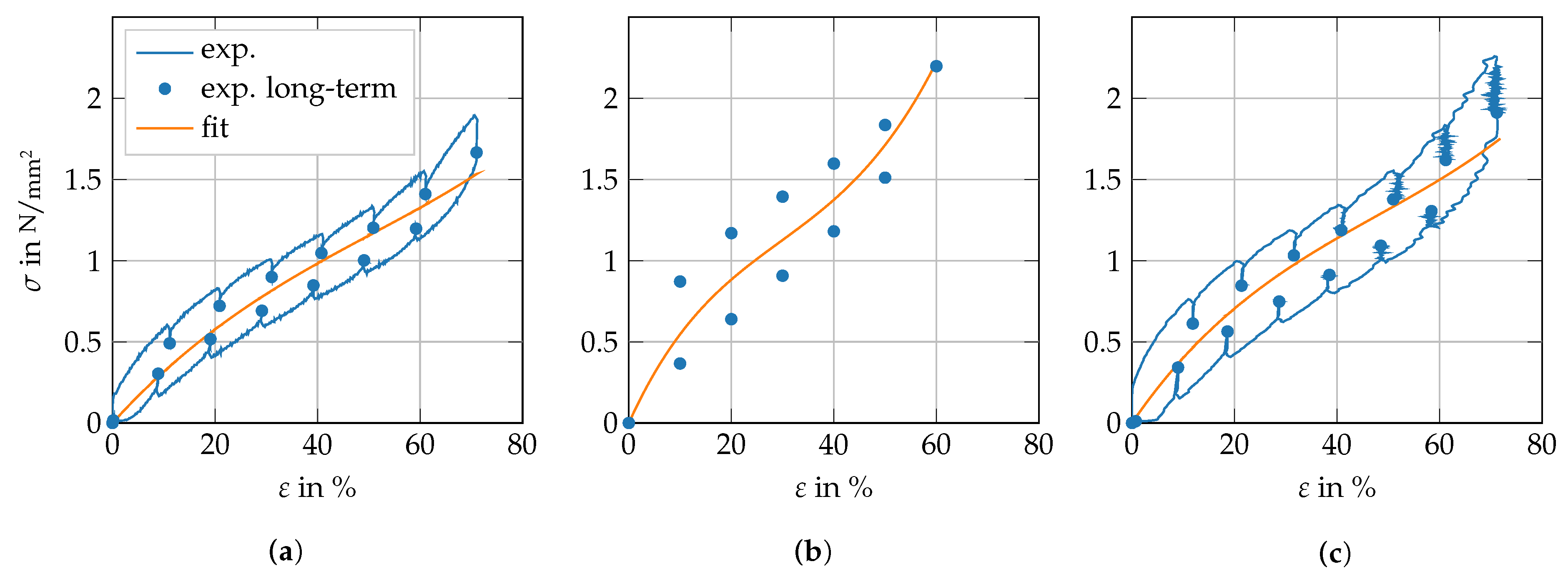
2.3.1. Identification of Elastic Parameters
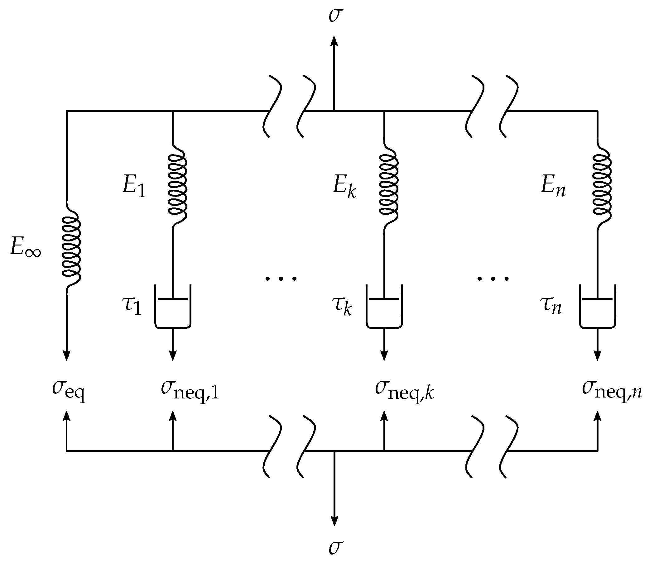
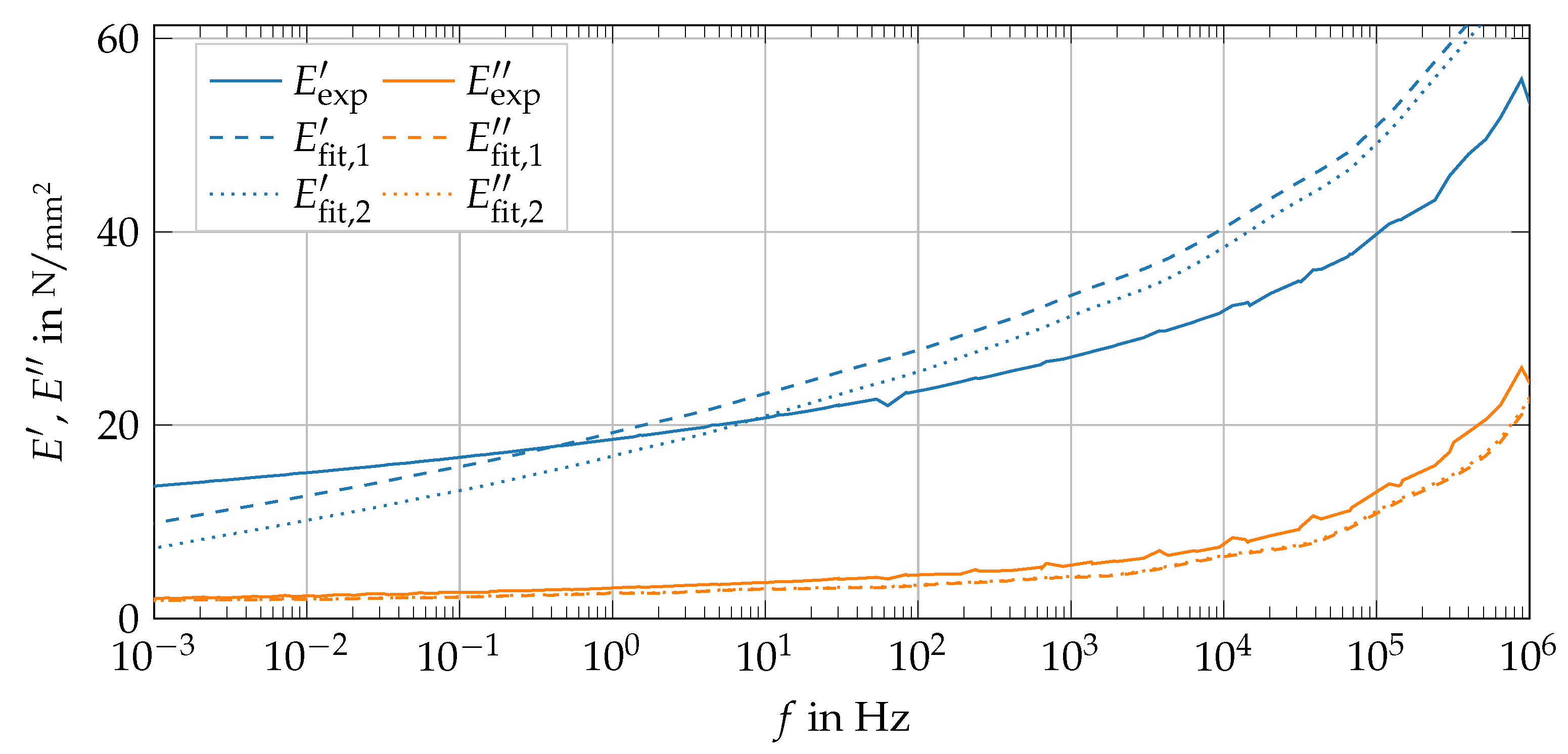
2.3.2. Identification of Viscoelastic Parameters
2.4. Wear Model
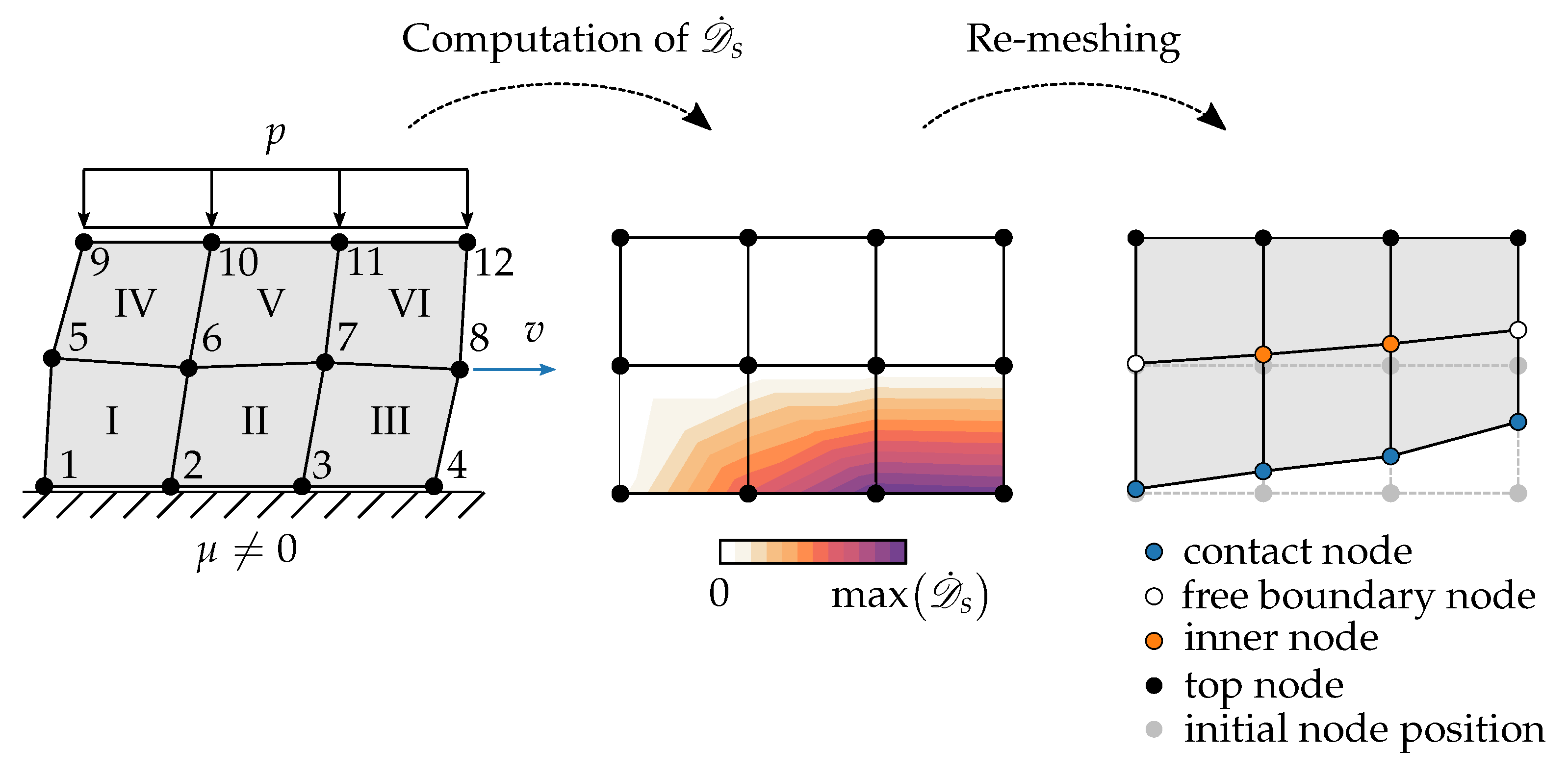
2.4.1. Post-Processing Re-Meshing Algorithm
2.4.2. Adaptive Meshing Algorithm
2.5. Image Processing and Mesh Generation
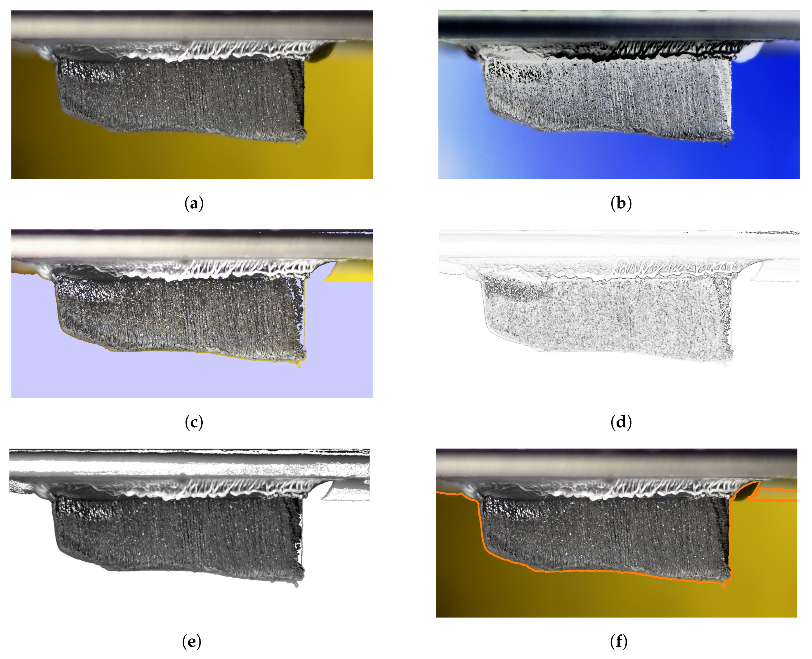
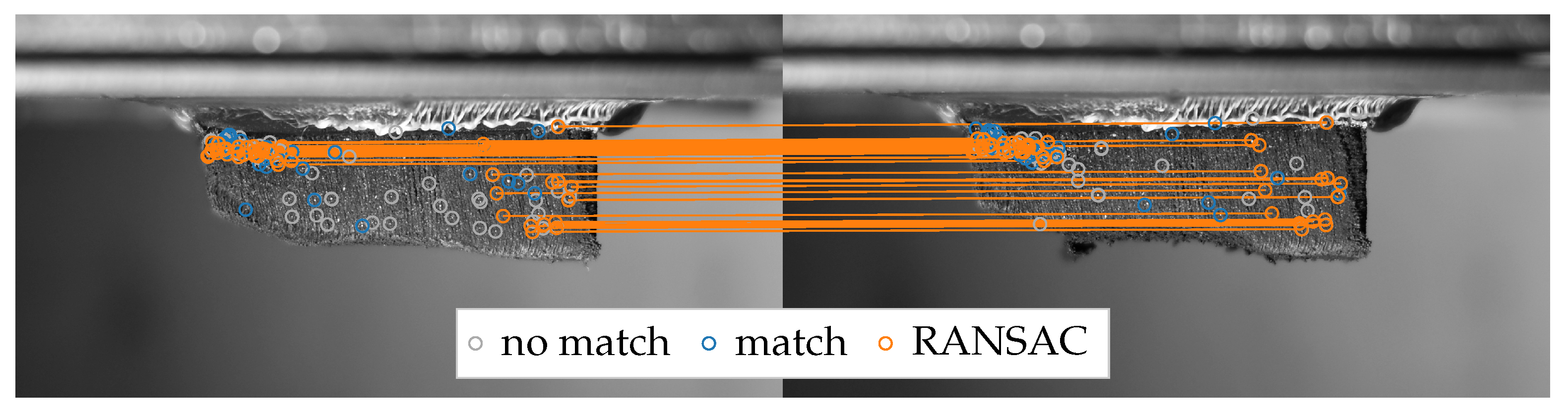
2.5.1. Image Processing
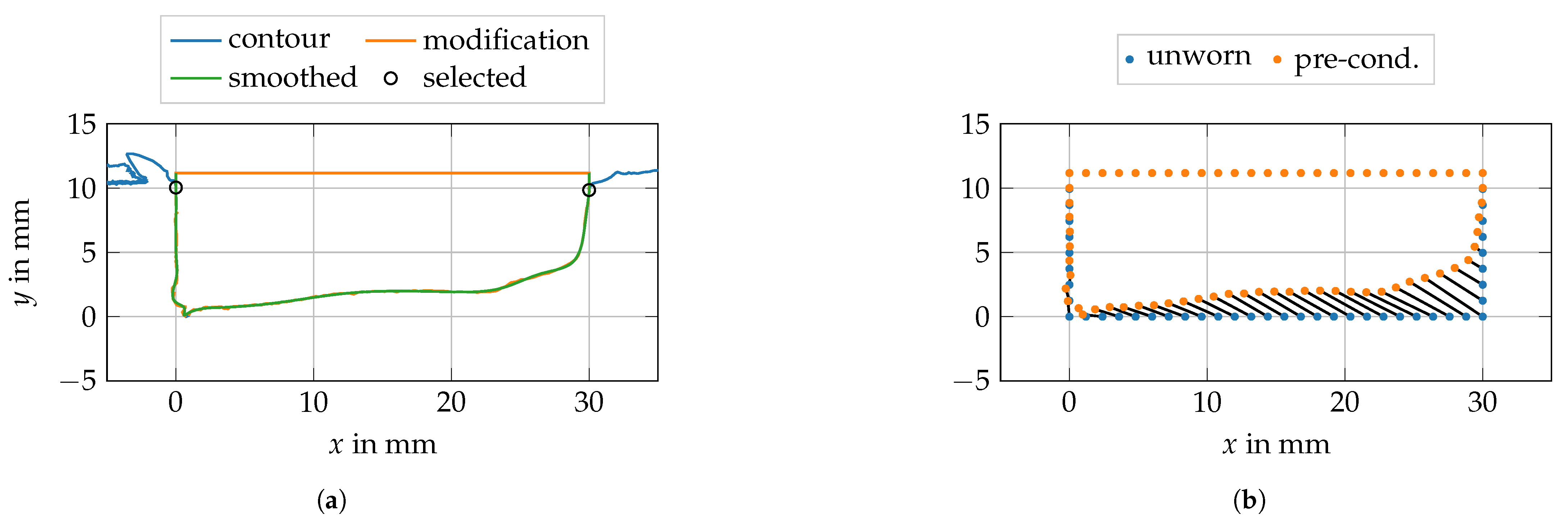
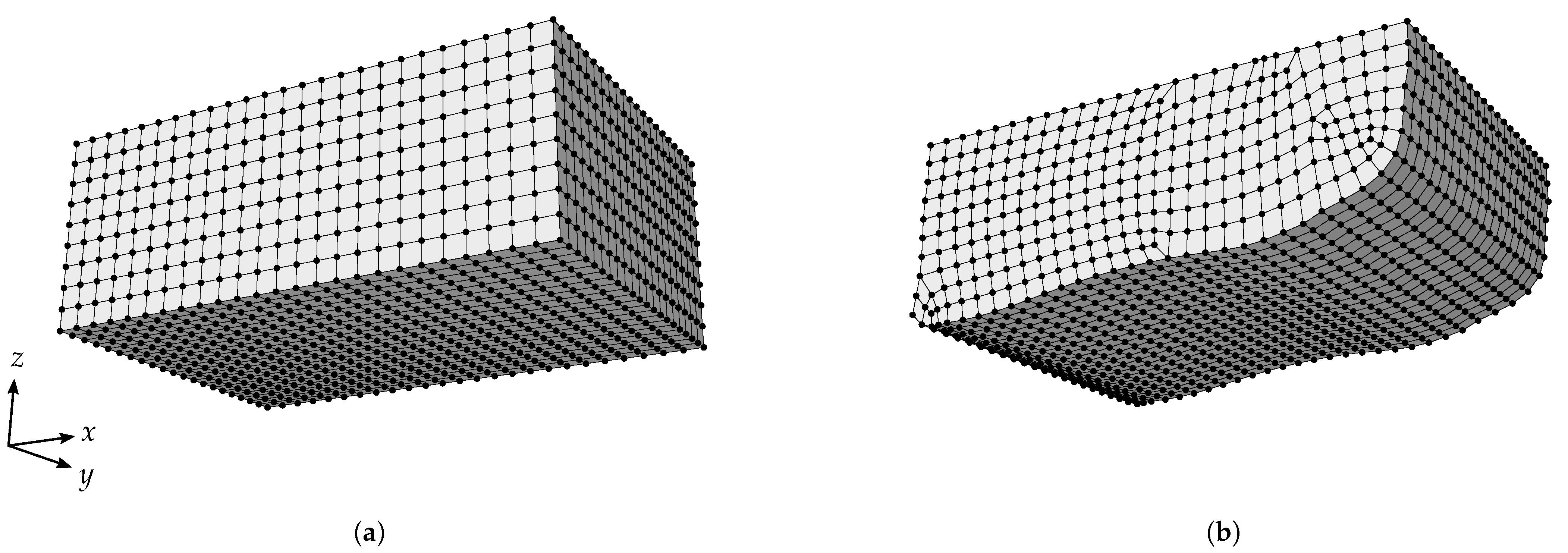
2.5.2. Mesh Generation
3. Results and Discussion
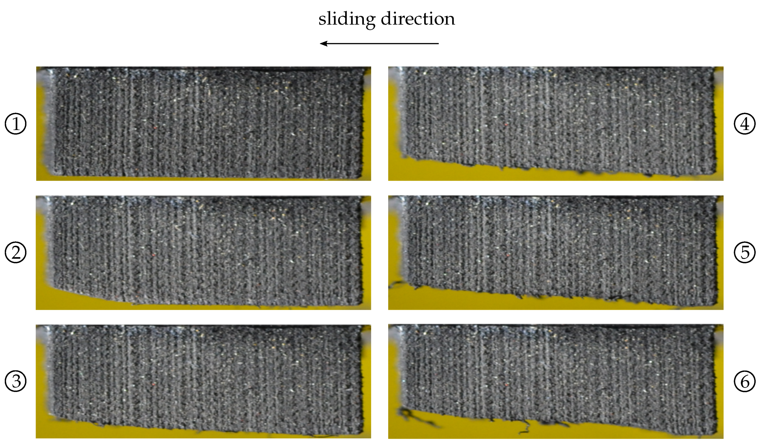
3.1. Experimental Output
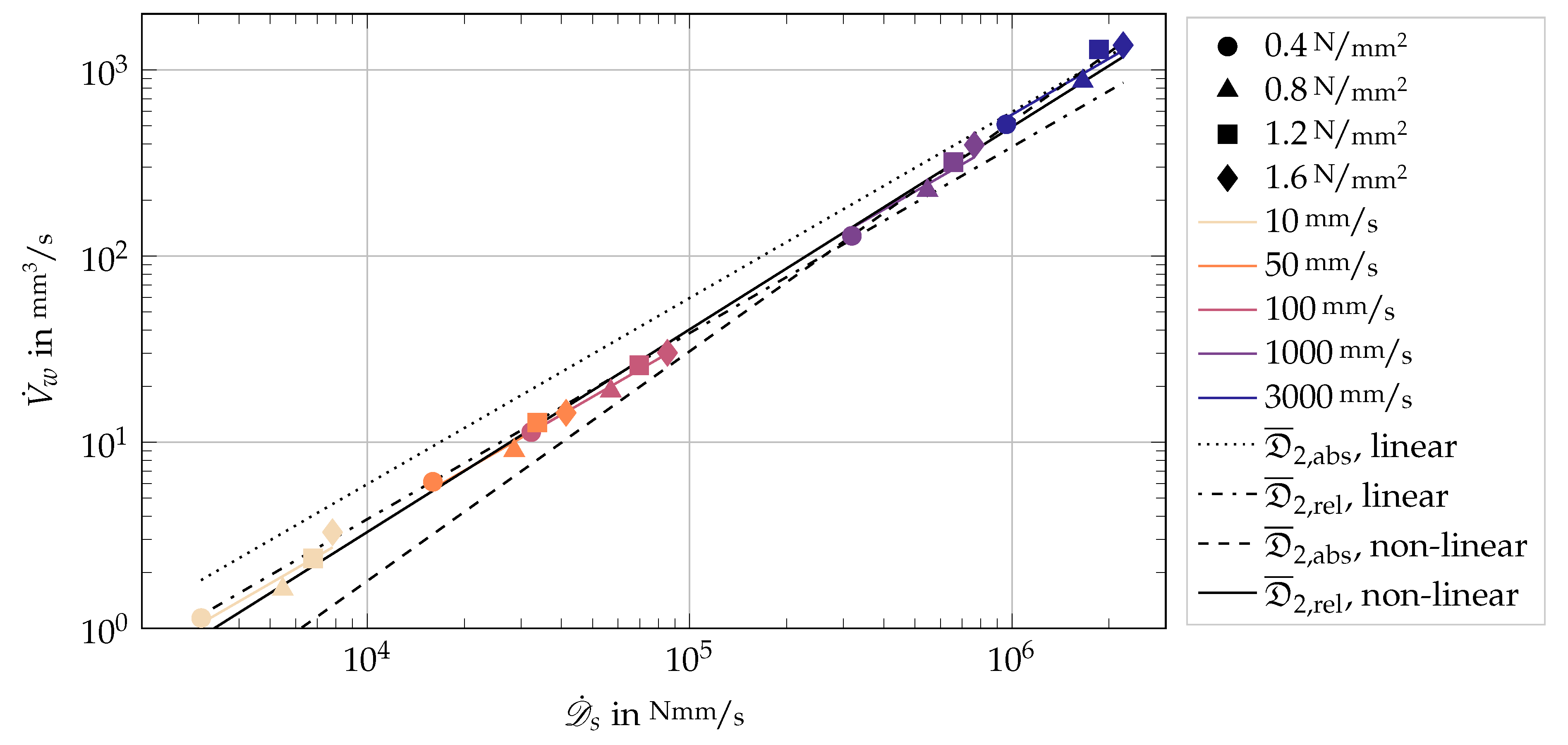
3.2. Wear Parameter Identification
3.3. Wear Simulation and Comparison to Experiments
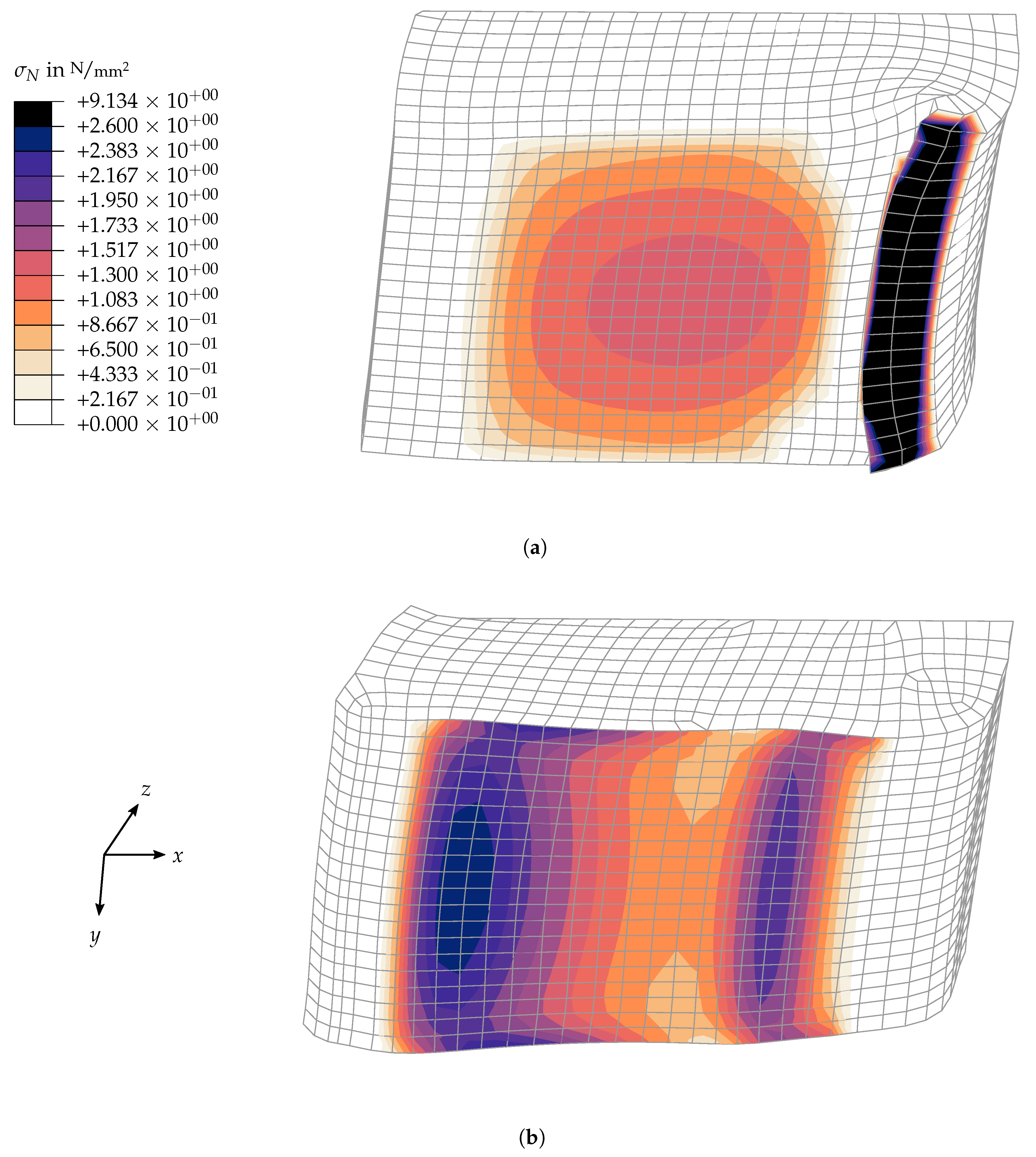
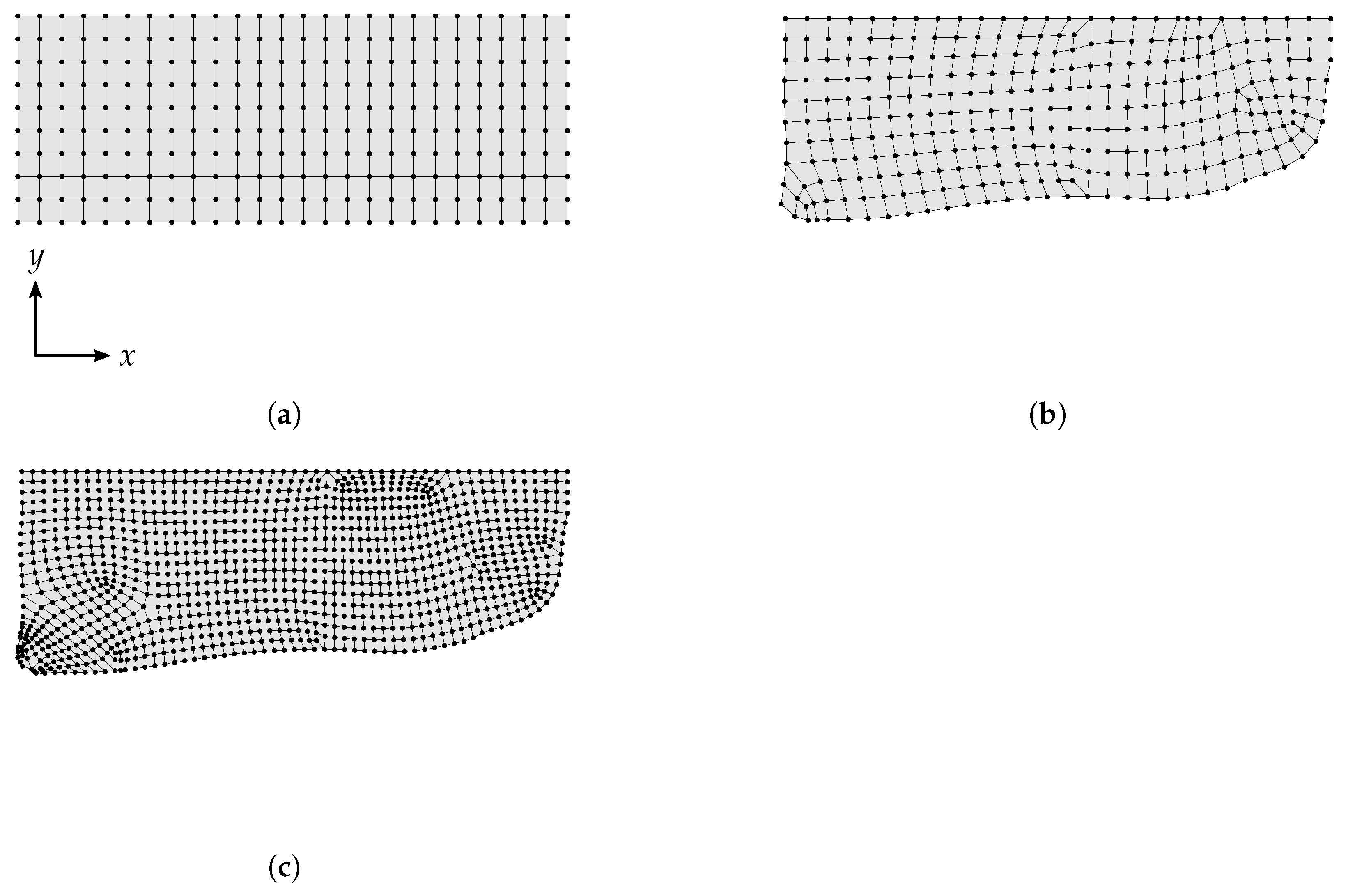
3.3.1. Wear Simulation
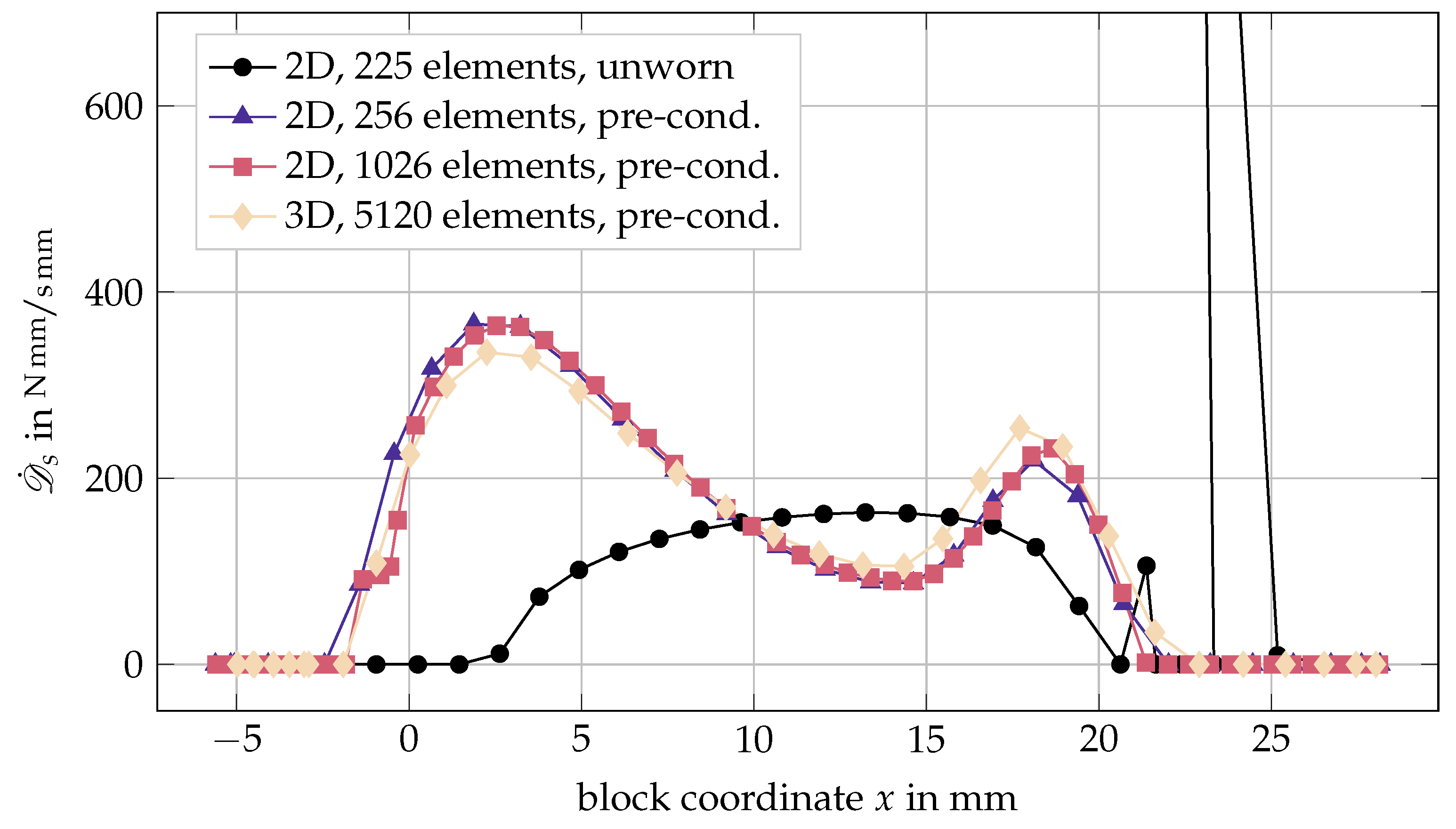
3.3.2. Verification
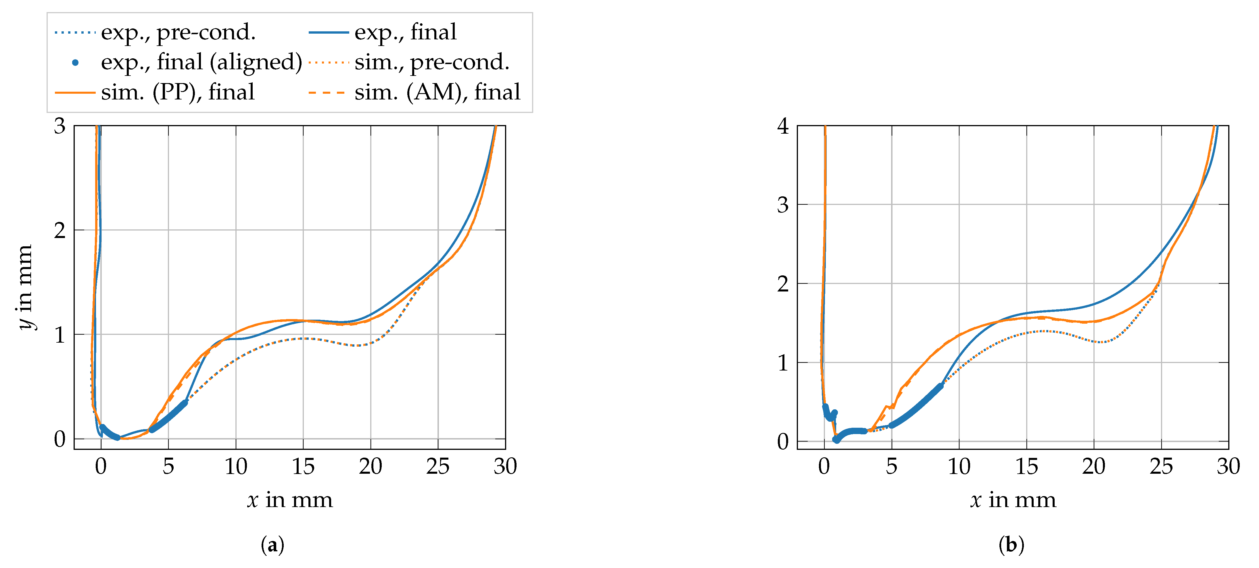
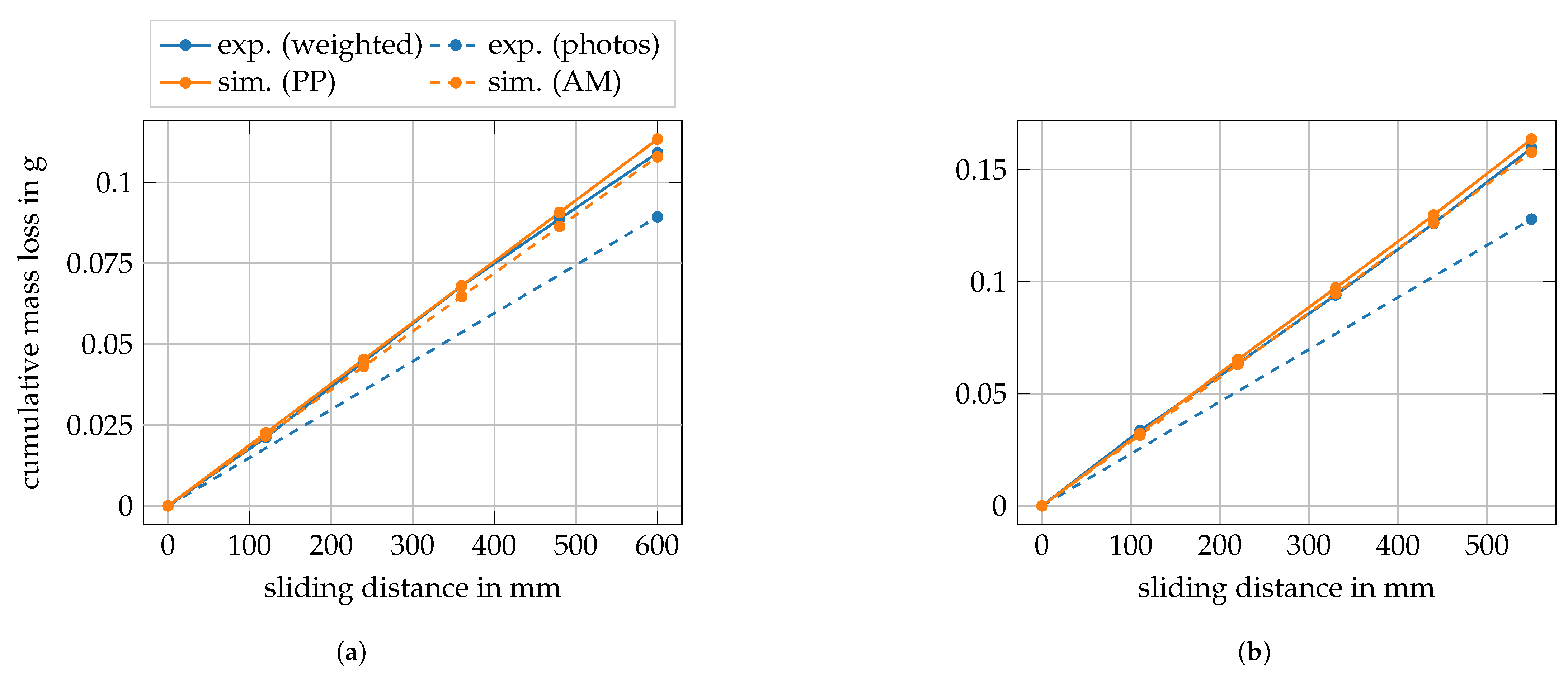
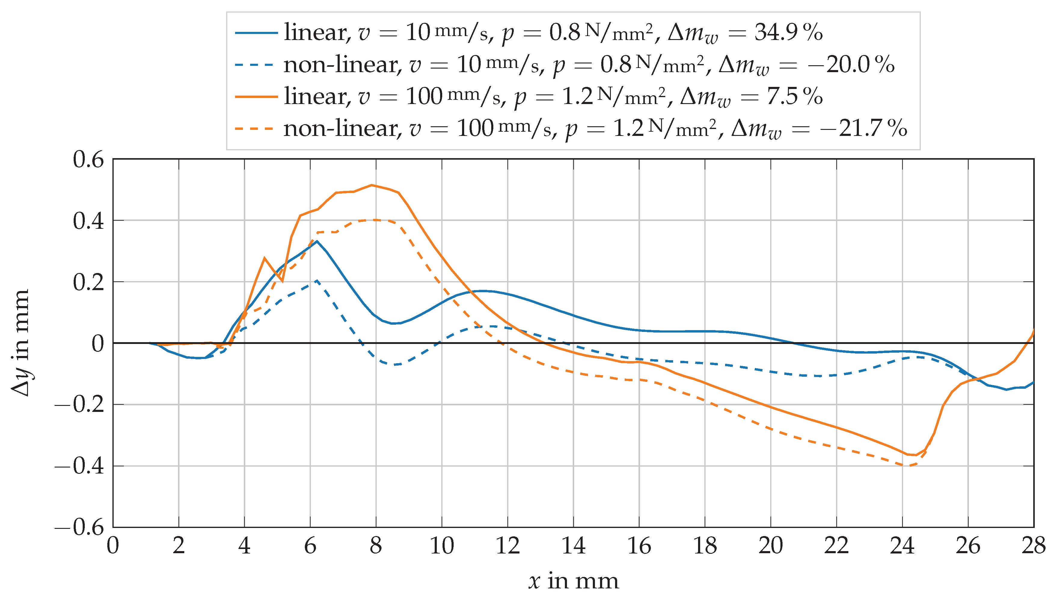
3.3.3. Validation
4. Conclusions
Author Contributions
Funding
Institutional Review Board Statement
Informed Consent Statement
Data Availability Statement
Acknowledgments
Conflicts of Interest
References
- Schulze, T.; Bolz, G.; Strübel, C.; Wies, B. Tire technology in target conflict of rolling resistance and wet grip. ATZ Worldw. 2010, 112, 26–32. [Google Scholar] [CrossRef]
- Baensch-Baltruschat, B.; Kocher, B.; Stock, F.; Reifferscheid, G. Tyre and road wear particles (TRWP)-A review of generation, properties, emissions, human health risk, ecotoxicity, and fate in the environment. Sci. Total Environ. 2020, 733, 137823. [Google Scholar] [CrossRef]
- Nguyen, V.; Zheng, D.; Schmerwitz, F.; Wriggers, P. An advanced abrasion model for tire wear. Wear 2018, 396, 75–85. [Google Scholar] [CrossRef]
- Li, Z.; Li, Z.; Wang, Y. An Integrated Approach for Friction and Wear Simulation of Tire Tread Rubber. Part II: Wear Test, Characterization and Modeling. Tire Sci. Technol. 2020, 48, 146–165. [Google Scholar] [CrossRef]
- Kahms, S.; Wangenheim, M. Experimental Investigation and Simulation of Aircraft Tire Wear. Tire Sci. Technol. 2021, 49, 55–74. [Google Scholar] [CrossRef]
- Pacejka, H. Tire and Vehicle Dynamics, 3rd ed.; Elsevier: Amsterdam, The Netherlands, 2012. [Google Scholar]
- Ripka, S.; Gäbel, G.; Wangenheim, M. Dynamics of a siped tire tread block-experiment and simulation. Tire Sci. Technol. 2009, 37, 323–339. [Google Scholar] [CrossRef]
- Genovese, A.; D’Angelo, G.A.; Sakhnevych, A.; Farroni, F. Review on friction and wear test rigs: An overview on the state of the art in tyre tread friction evaluation. Lubricants 2020, 8, 91. [Google Scholar] [CrossRef]
- Rosu, I.; Elias-Birembaux, H.L.; Lebon, F.; Lind, H.; Wangenheim, M. Experimental and numerical simulation of the dynamic frictional contact between an aircraft tire rubber and a rough surface. Lubricants 2016, 4, 29. [Google Scholar] [CrossRef] [Green Version]
- Zheng, D. Prediction of tire tread wear with FEM steady state rolling contact simulation. Tire Sci. Technol. 2003, 31, 189–202. [Google Scholar] [CrossRef]
- Hegadekatte, V.; Huber, N.; Kraft, O. Finite element based simulation of dry sliding wear. Model. Simul. Mater. Sci. Eng. 2004, 13, 57. [Google Scholar] [CrossRef]
- Runge, S.; Ignatyev, P.; Wangenheim, M.; Bederna, C.; Wies, B.; Wallaschek, J. Transient abrasion on a rubber sample due to highly dynamic contact conditions. Wear 2021, 203848. [Google Scholar] [CrossRef]
- Moldenhauer, P.; Kröger, M. Simulation and experimental investigations of the dynamic interaction between tyre tread block and road. In Elastomere Friction: Theory, Experiment and Simulation; Springer: Berlin/Heidelberg, Germany, 2010; pp. 165–200. [Google Scholar] [CrossRef]
- Kaliske, M.; Rothert, H. Formulation and implementation of three-dimensional viscoelasticity at small and finite strains. Comput. Mech. 1997, 19, 228–239. [Google Scholar] [CrossRef]
- Holzapfel, G.A. Nonlinear Solid Mechanics: A Continuum Approach for Engineering; Wiley: Chichester, UK, 2000. [Google Scholar]
- Yeoh, O. Characterization of Elastic Properties of Carbon-Black-Filled Rubber Vulcanizates. Rubber Chem. Technol. 1990, 63, 792–805. [Google Scholar] [CrossRef]
- Rackl, M. Curve Fitting for Ogden, Yeoh and Polynomial Models. In Proceedings of the 7th International Scilab Users Conference, Paris, France, 21–22 May 2015. [Google Scholar]
- Gent, A.; Pulford, C. Mechanisms of Rubber Abrasion. J. Appl. Polym. Sci. 1983, 28, 943–960. [Google Scholar] [CrossRef]
- Archard, J.F. Contact and rubbing of flat surfaces. J. Appl. Phys. 1953, 24, 981–988. [Google Scholar] [CrossRef]
- Schallamach, A.; Turner, D. The wear of slipping wheels. Wear 1960, 3, 1–25. [Google Scholar] [CrossRef]
- Li, Z.; Li, Z.; Wang, Y. An Integrated Approach for Friction and Wear Simulation of Tire Tread Rubber. Part I: Friction Test, Characterization and Modeling. Tire Sci. Technol. 2020, 48, 123–145. [Google Scholar] [CrossRef]
- Wriggers, P. Computational Contact Mechanics; Springer: Berlin/Heidelberg, Germany, 2006. [Google Scholar] [CrossRef]
- Walt, S.v.d.; Schönberger, J.L.; Nunez-Iglesias, J.; Boulogne, F.; Warner, J.D.; Yager, N.; Gouillart, E.; Yu, T. scikit-image: Image processing in Python. PeerJ 2014, 2, e453. [Google Scholar] [CrossRef]
- Available online: http://www.janeriksolem.net/histogram-equalization-with-python-and.html (accessed on 23 April 2021).
- Sobel, I.; Feldman, G. An Isotropic 3 × 3 Image Gradient Operator. Presentation at Stanford A.I. Project. 1968. Available online: https://www.researchgate.net/publication/239398674_An_Isotropic_3x3_Image_Gradient_Operator/citation/download (accessed on 23 April 2021).
- Lorensen, W.E.; Cline, H.E. Marching cubes: A high resolution 3D surface construction algorithm. ACM Siggraph Comput. Graph. 1987, 21, 163–169. [Google Scholar] [CrossRef]
- Rublee, E.; Rabaud, V.; Konolige, K.; Bradski, G. ORB: An efficient alternative to SIFT or SURF. In Proceedings of the 2011 International Conference on Computer Vision, Barcelona, Spain, 6–13 November 2011; pp. 2564–2571. [Google Scholar] [CrossRef]
- Fischler, M.A.; Bolles, R.C. Random sample consensus: A paradigm for model fitting with applications to image analysis and automated cartography. Commun. Assoc. Comput. Mach. 1981, 24, 381–395. [Google Scholar] [CrossRef]
- Dierckx, P. Algorithms for smoothing data with periodic and parametric splines. Comput. Graph. Image Process. 1982, 20, 171–184. [Google Scholar] [CrossRef]
- Simo, J.; Laursen, T. An augmented lagrangian treatment of contact problems involving friction. Comput. Struct. 1992, 42, 97–116. [Google Scholar] [CrossRef]


| Branch k | ||
|---|---|---|
| 1 | ||
| 2 | ||
| 3 | ||
| 4 | ||
| 5 | ||
| 6 | ||
| 7 | ||
| 8 | ||
| 9 | ||
| 10 | ||
| 11 | ||
| 12 | ||
| 13 | ||
| 14 | ||
| 15 |
| Parameter | Linear (abs. Error) | Linear (rel. Error) | Non-Linear (abs. Error) | Non-Linear (rel. Error) |
|---|---|---|---|---|
| in | ||||
| 1 | 1 | 1.234 | 1.089 | |
| 0.978 | 0.808 | 0.988 | 0.961 |
| Number | Name | Description | Boundary Conditions |
|---|---|---|---|
| 1 | Contact | Counter surface is lifted to ensure contact between rubber block and bottom rigid surface | |
| 2 | Loading | Counter surface is pressed against rubber block | |
| 3 | Ramping | Counter surface is accelerated while friction is continuously increased | |
| 4 | Sliding-on-aluminum | Counter surface is moving with constant speed and aluminum based friction | |
| 5 | Sliding-on-sandpaper | Counter surface is moving with constant speed and sandpaper based friction |
Publisher’s Note: MDPI stays neutral with regard to jurisdictional claims in published maps and institutional affiliations. |
© 2021 by the authors. Licensee MDPI, Basel, Switzerland. This article is an open access article distributed under the terms and conditions of the Creative Commons Attribution (CC BY) license (https://creativecommons.org/licenses/by/4.0/).
Share and Cite
Hartung, F.; Garcia, M.A.; Berger, T.; Hindemith, M.; Wangenheim, M.; Kaliske, M. Experimental and Numerical Investigation of Tire Tread Wear on Block Level. Lubricants 2021, 9, 113. https://doi.org/10.3390/lubricants9120113
Hartung F, Garcia MA, Berger T, Hindemith M, Wangenheim M, Kaliske M. Experimental and Numerical Investigation of Tire Tread Wear on Block Level. Lubricants. 2021; 9(12):113. https://doi.org/10.3390/lubricants9120113
Chicago/Turabian StyleHartung, Felix, Mario Alejandro Garcia, Thomas Berger, Michael Hindemith, Matthias Wangenheim, and Michael Kaliske. 2021. "Experimental and Numerical Investigation of Tire Tread Wear on Block Level" Lubricants 9, no. 12: 113. https://doi.org/10.3390/lubricants9120113
APA StyleHartung, F., Garcia, M. A., Berger, T., Hindemith, M., Wangenheim, M., & Kaliske, M. (2021). Experimental and Numerical Investigation of Tire Tread Wear on Block Level. Lubricants, 9(12), 113. https://doi.org/10.3390/lubricants9120113