A Mixed Elasto-Hydrodynamic Lubrication Model for Wear Calculation in Artificial Hip Joints


Abstract
:
1. Introduction
- -
- The progressive wear phenomenon in the lubricating gap calculation through a modified Archard law;
- -
- The non-Newtonian synovial fluid behavior through the cross-viscosity model;
- -
- The cup surface deflection using a constrained column model.
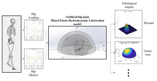
2. Materials and Methods
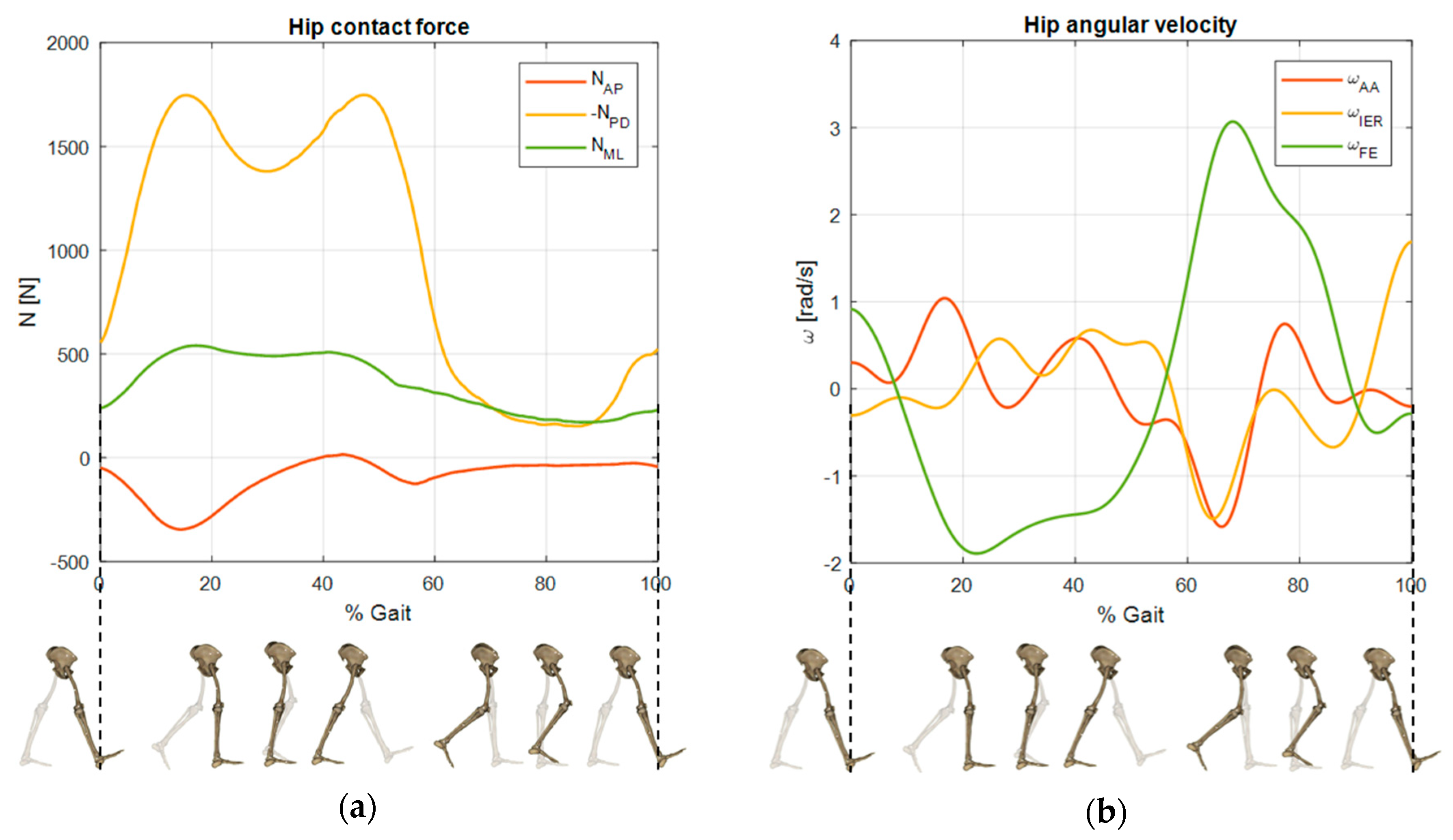
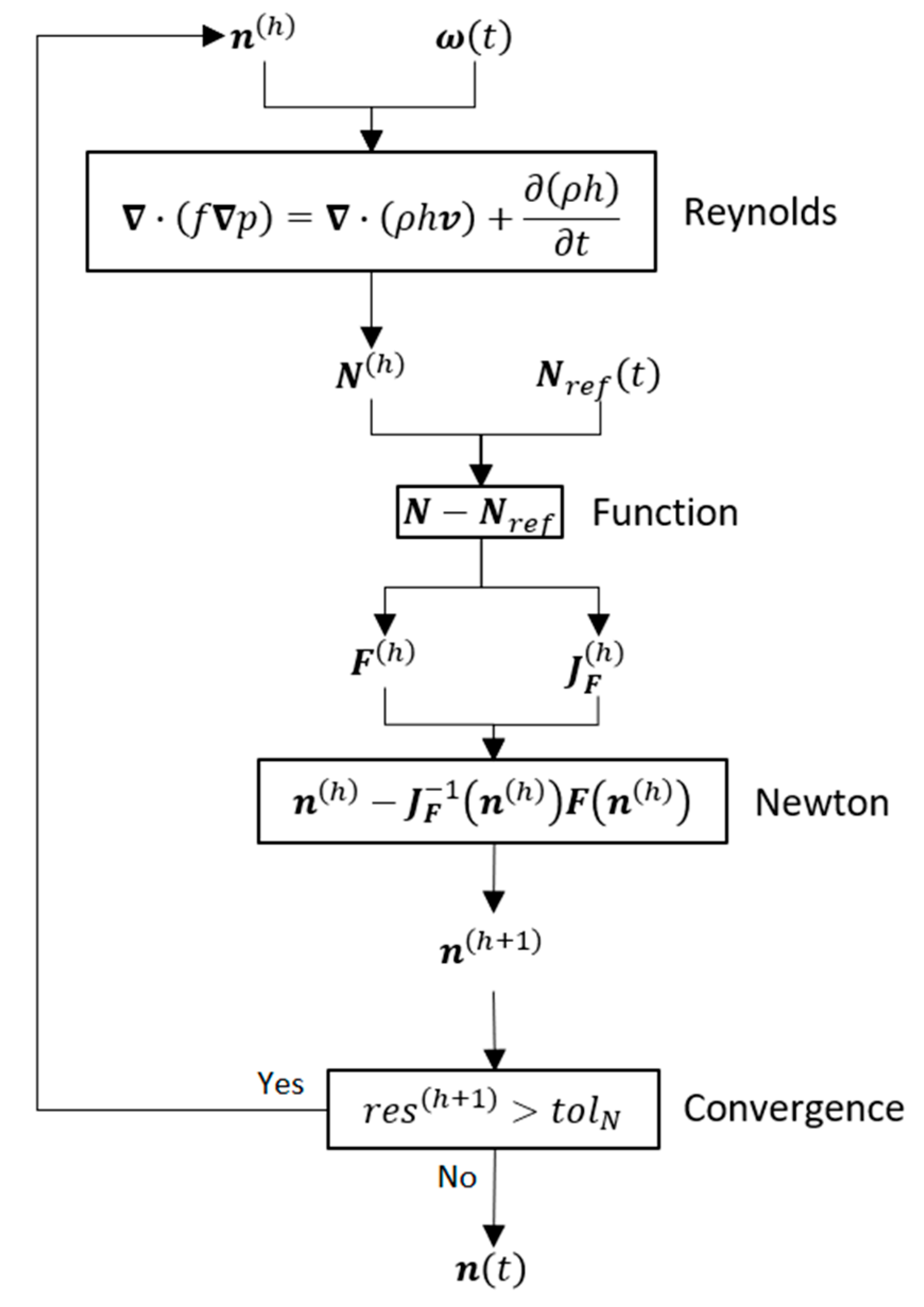
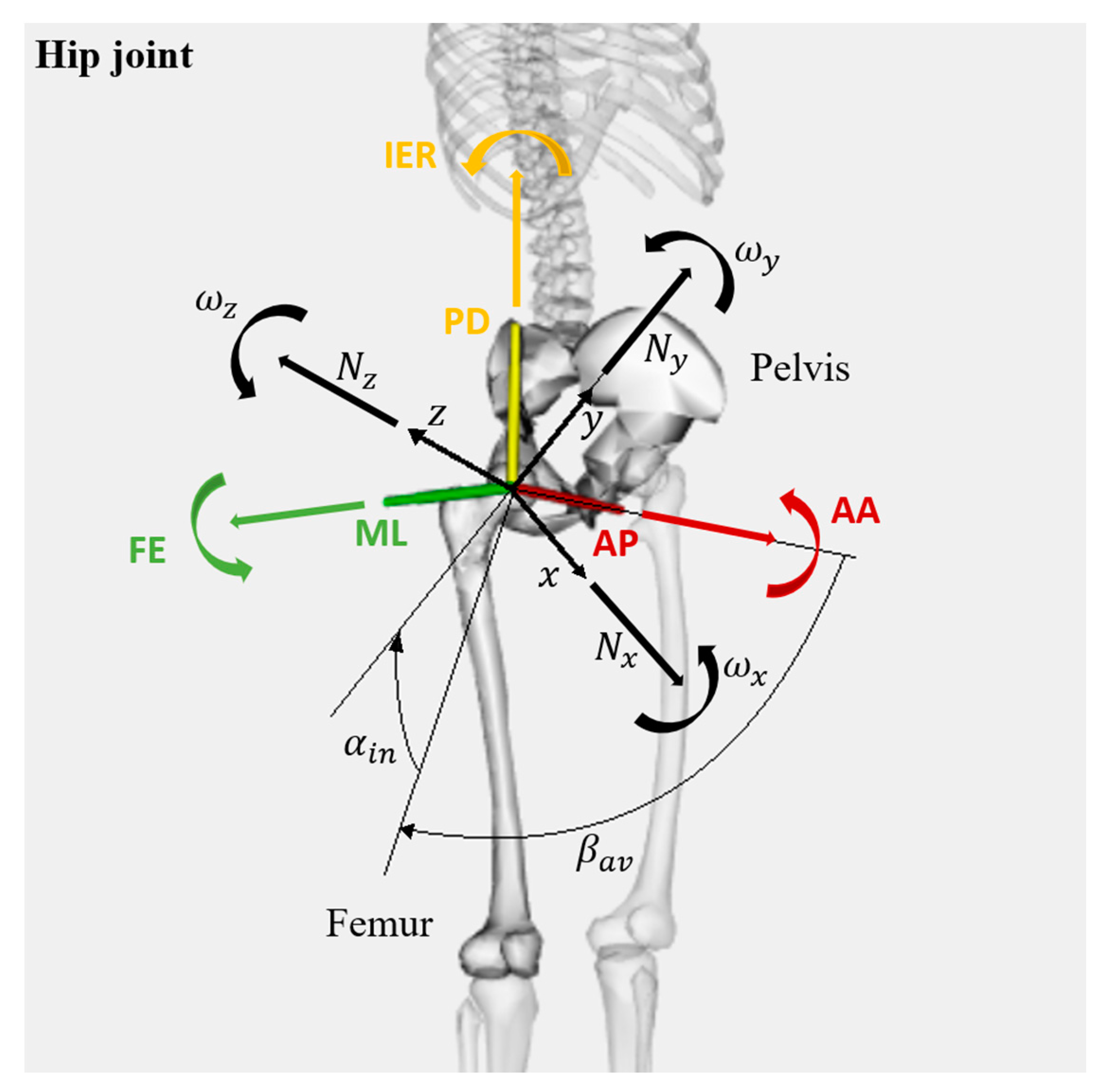
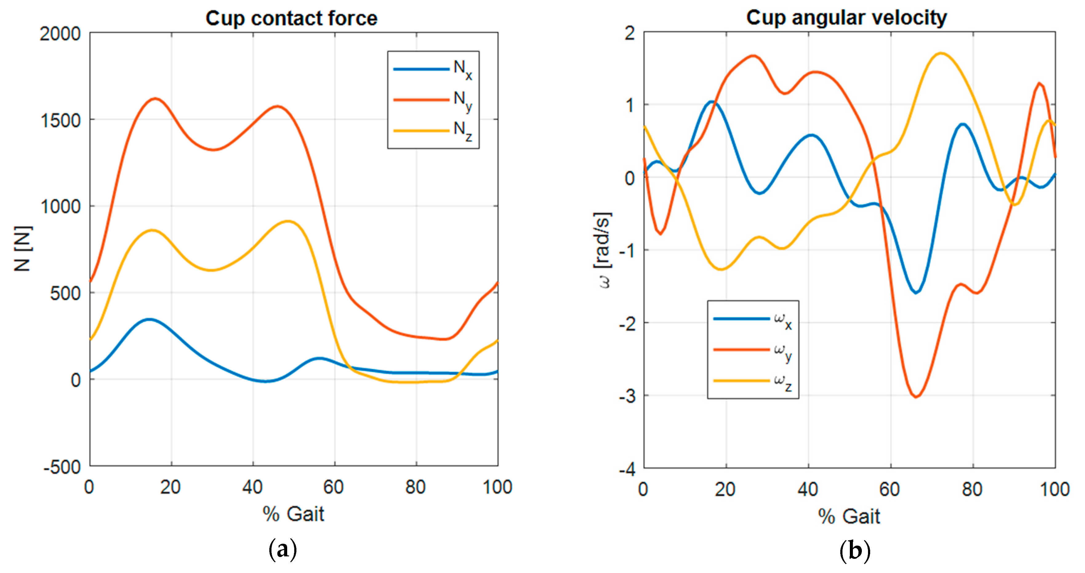
2.1. The Hip Joint during the Gait
- -
- The Flexion–Extension rotation (FE) around the Medio–Lateral axis (ML) perpendicular to the sagittal plane;
- -
- The Adduction–Abduction rotation (AA) around the Anterior–Posterior axis (AP) perpendicular to the frontal plane;
- -
- The Internal–External Rotation (IER) around the Proximo–Distal axis (PD) perpendicular to the horizontal plane.
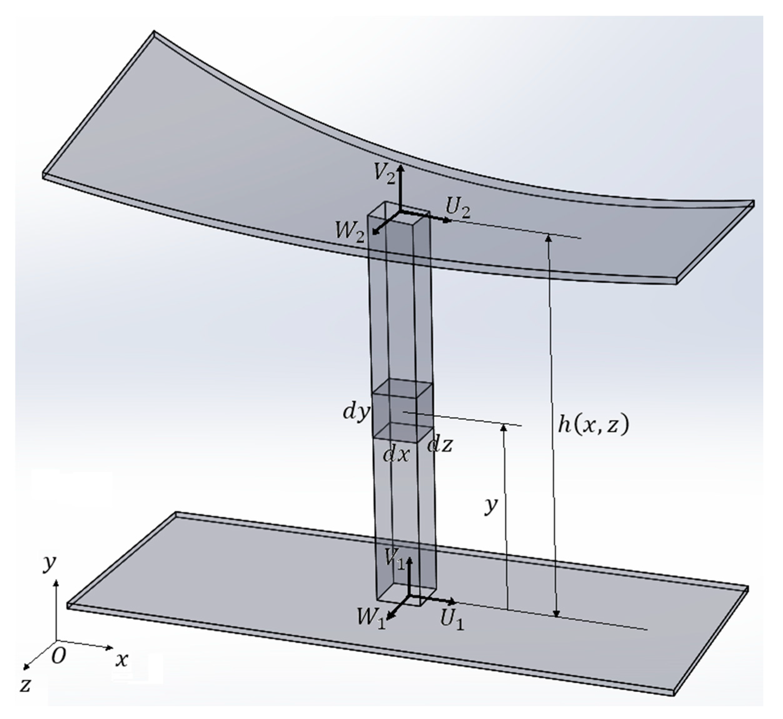
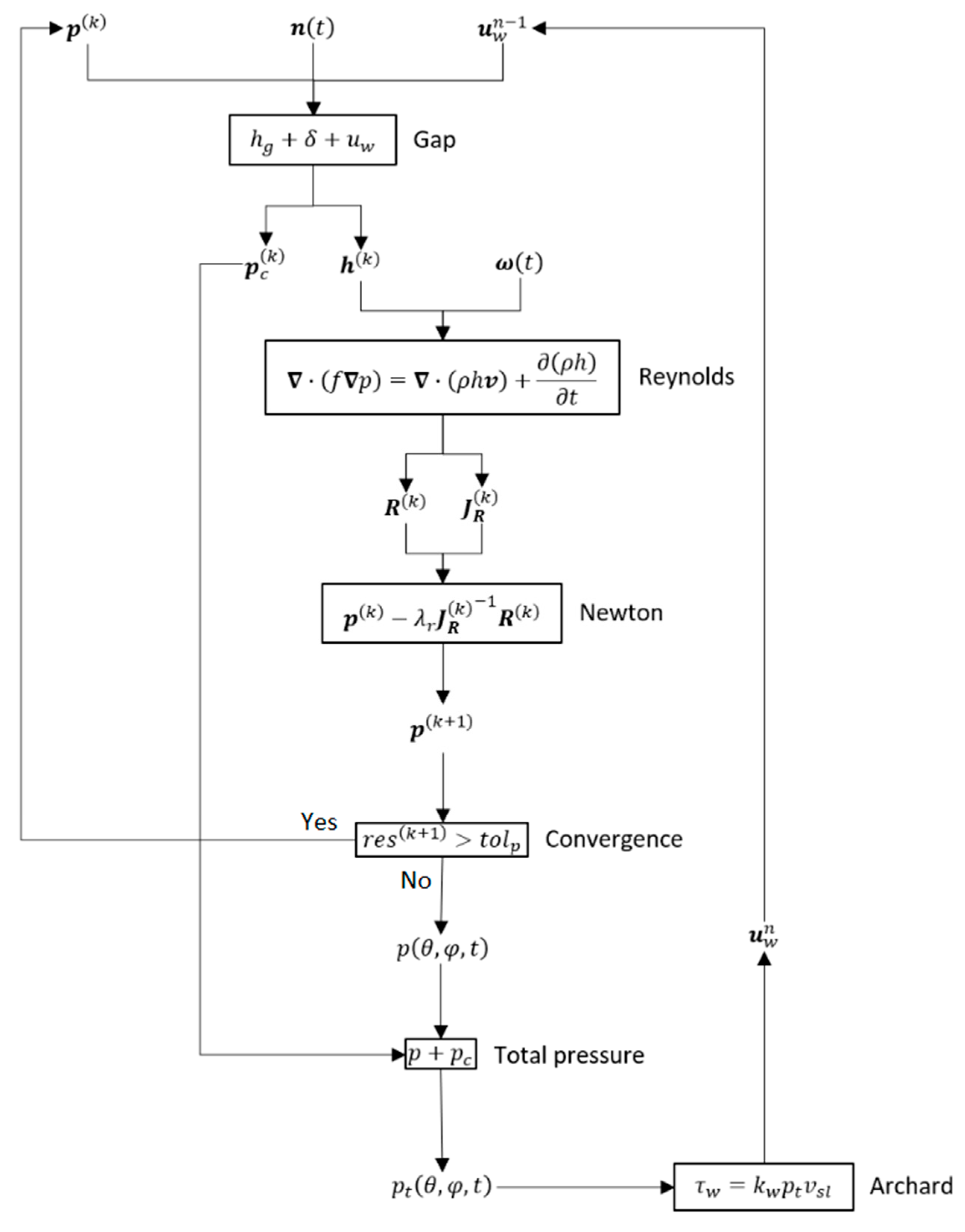
2.2. The Modified Reynolds Lubrication Equation
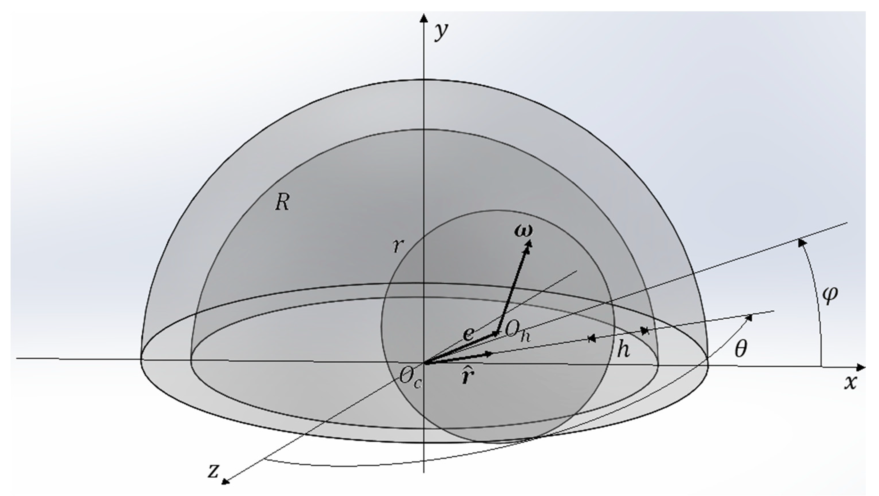
2.3. The Spherical Joint
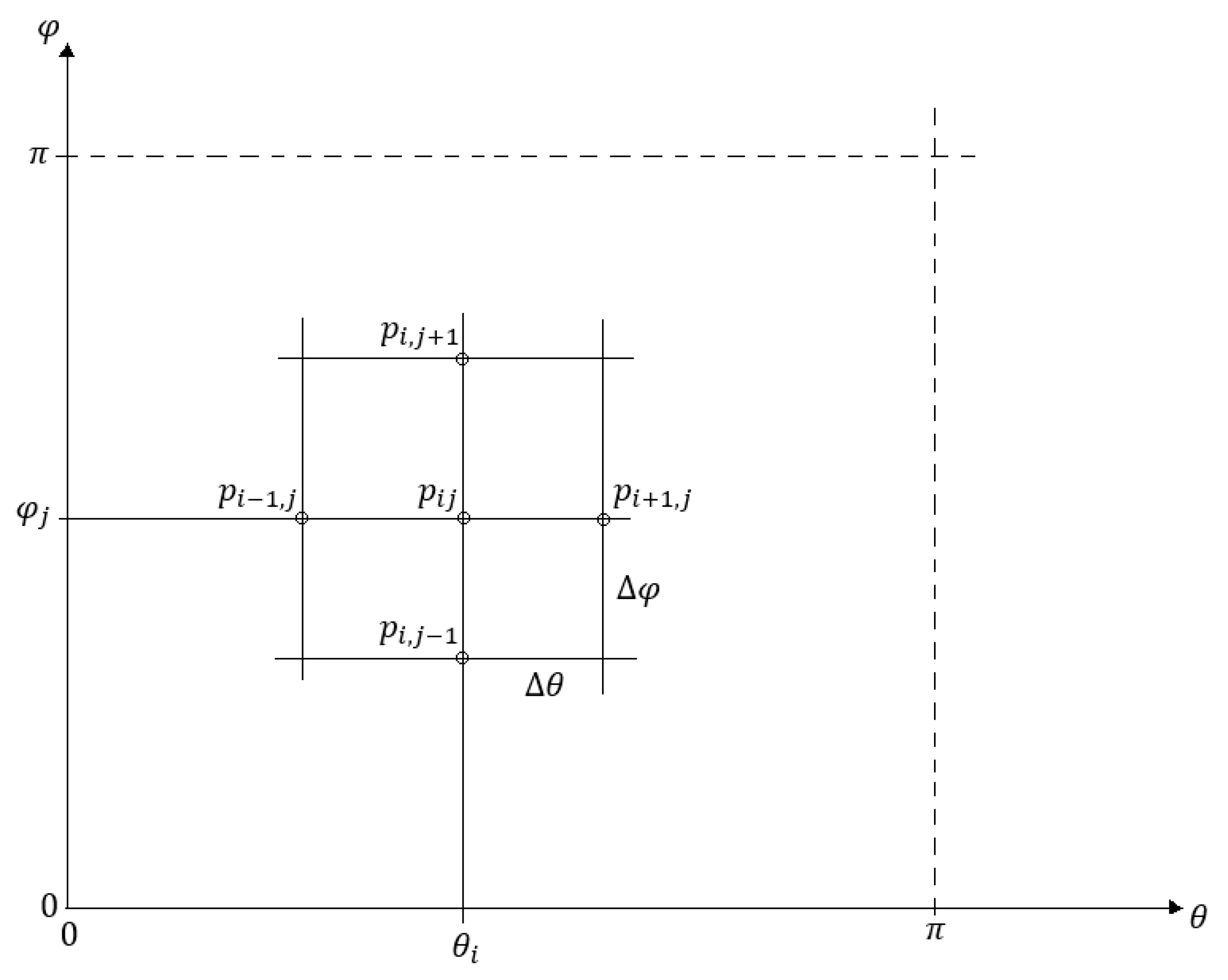
2.4. Discrete Reynolds Equation
3. Results and Discussion
- -
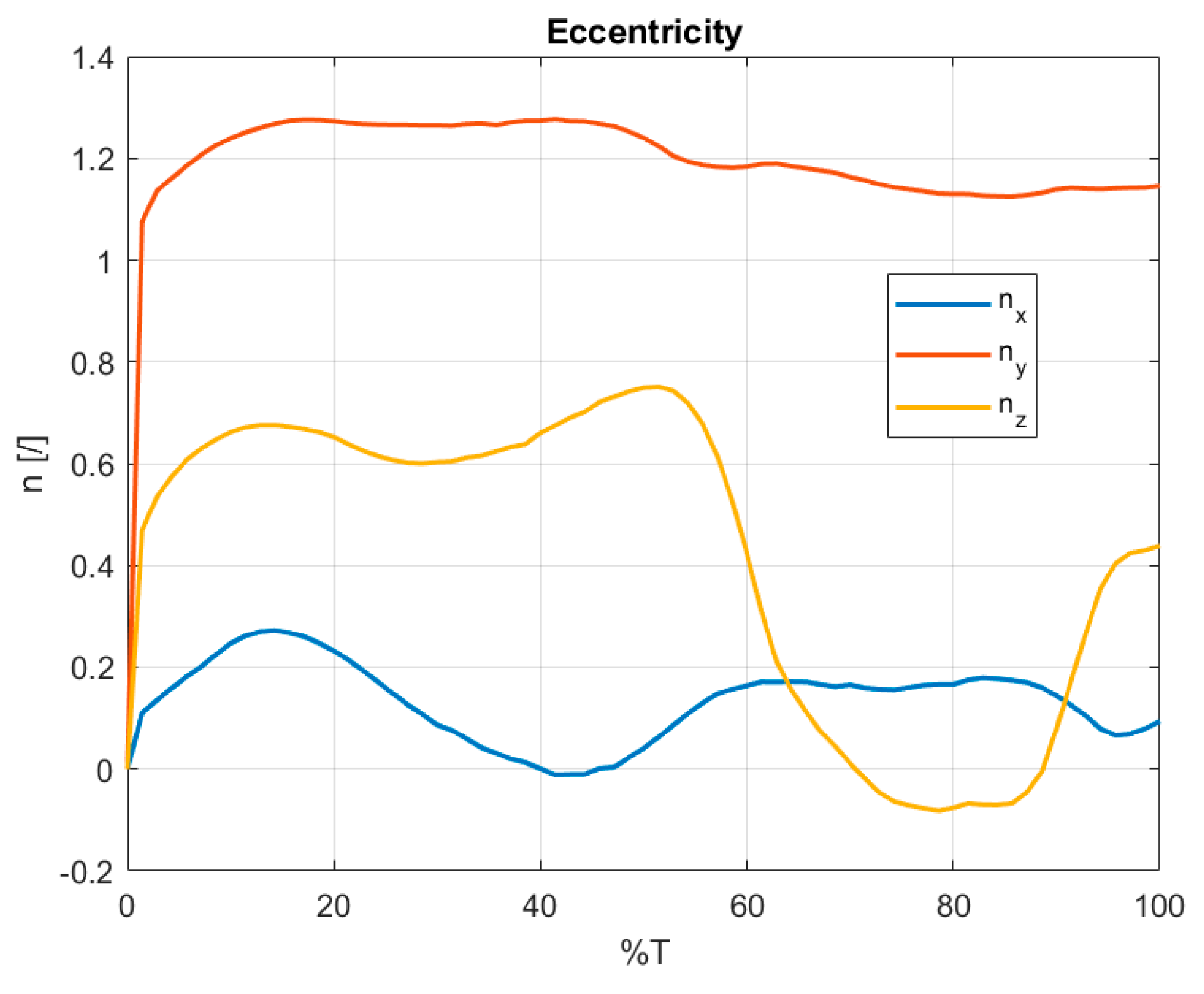
- Only the time evolution of the component of the dimensionless eccentricity from 0 to 1.1 over 0.1 s;
- -
- Only the time evolution of the component of the angular velocity as a constant value equal to 500 rad/s, so that a faster relative sliding motion was considered.
4. Conclusions
- -
- -
- -
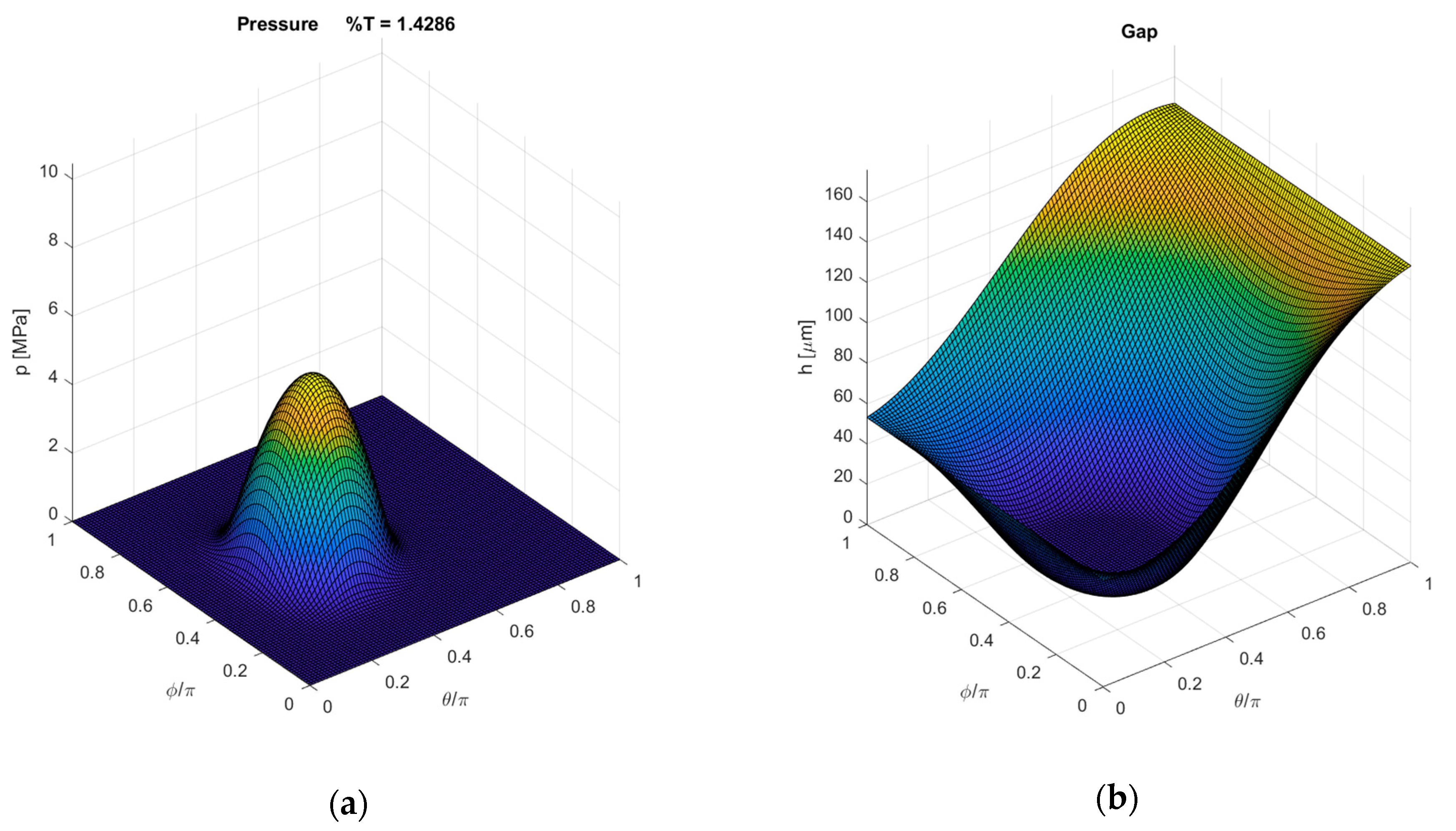
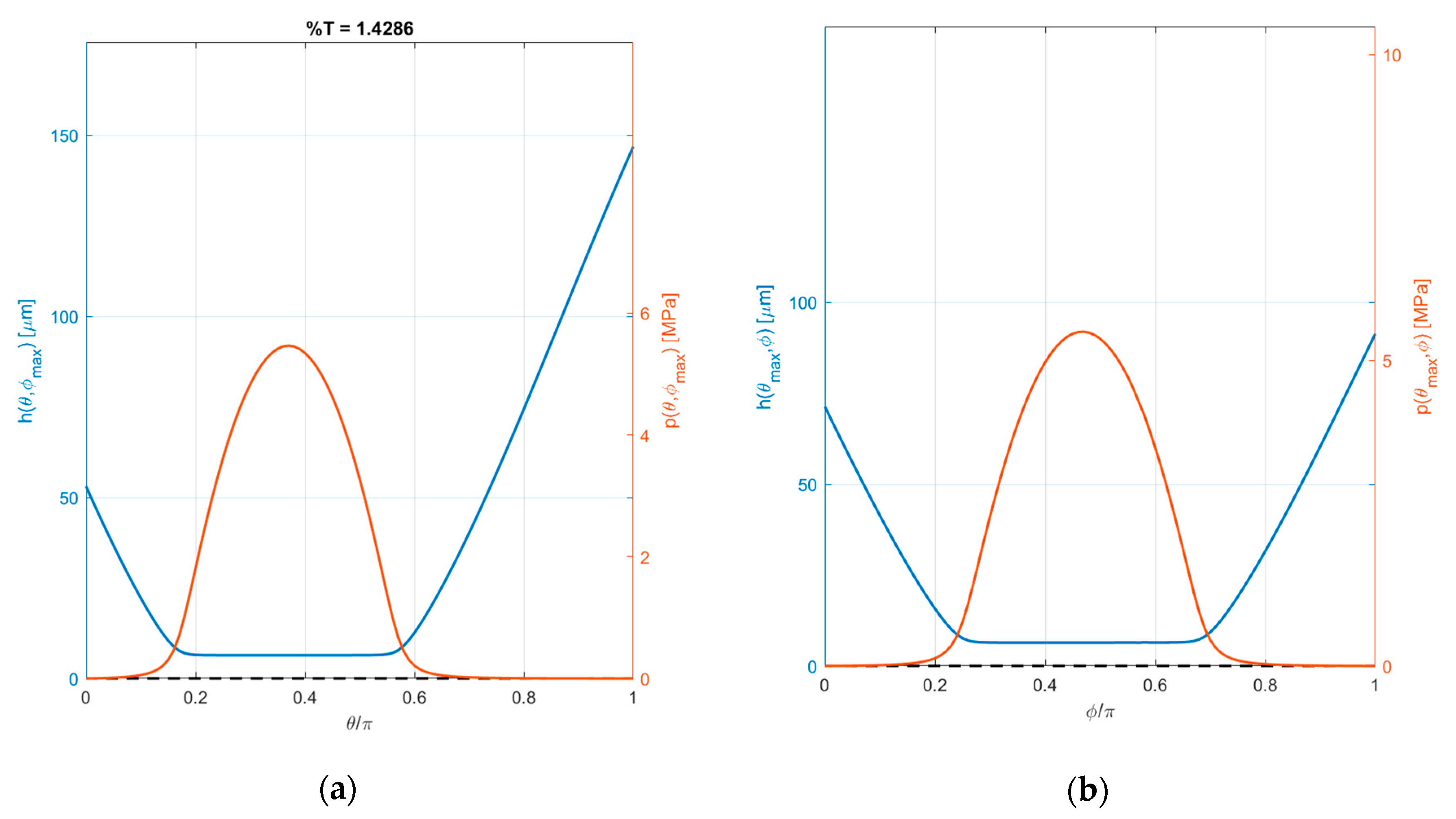
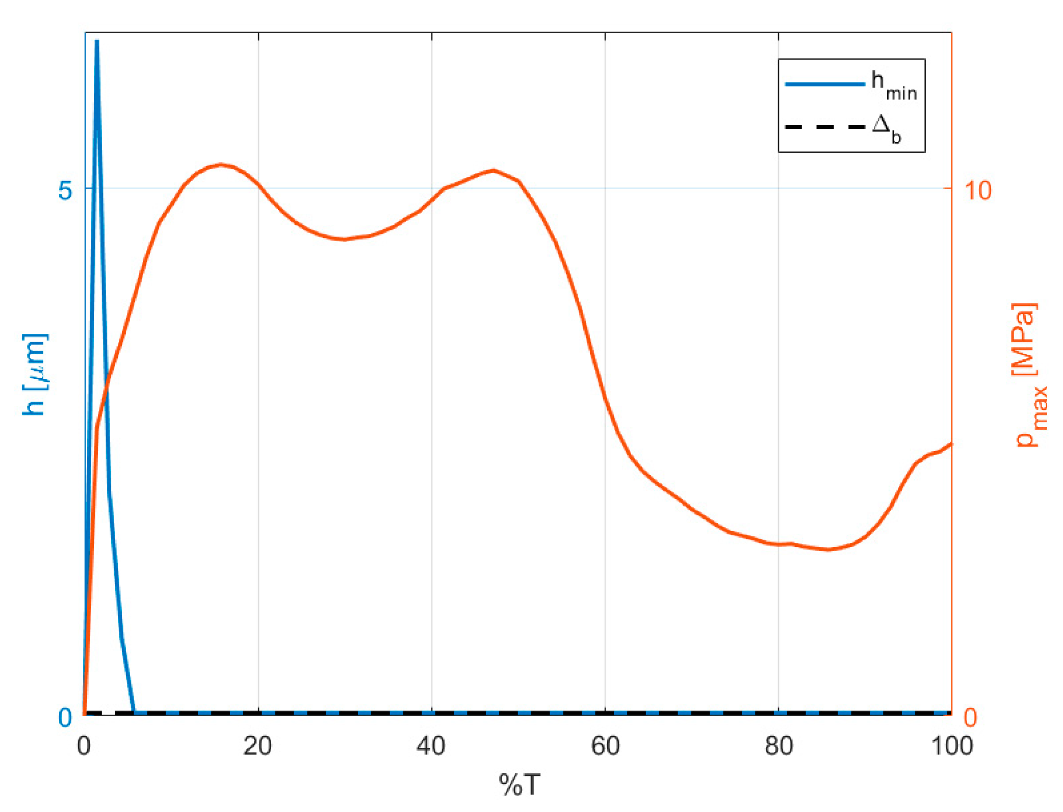
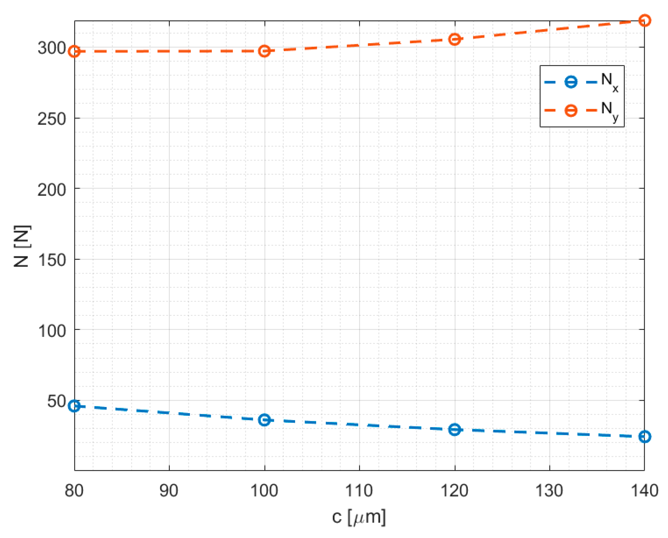
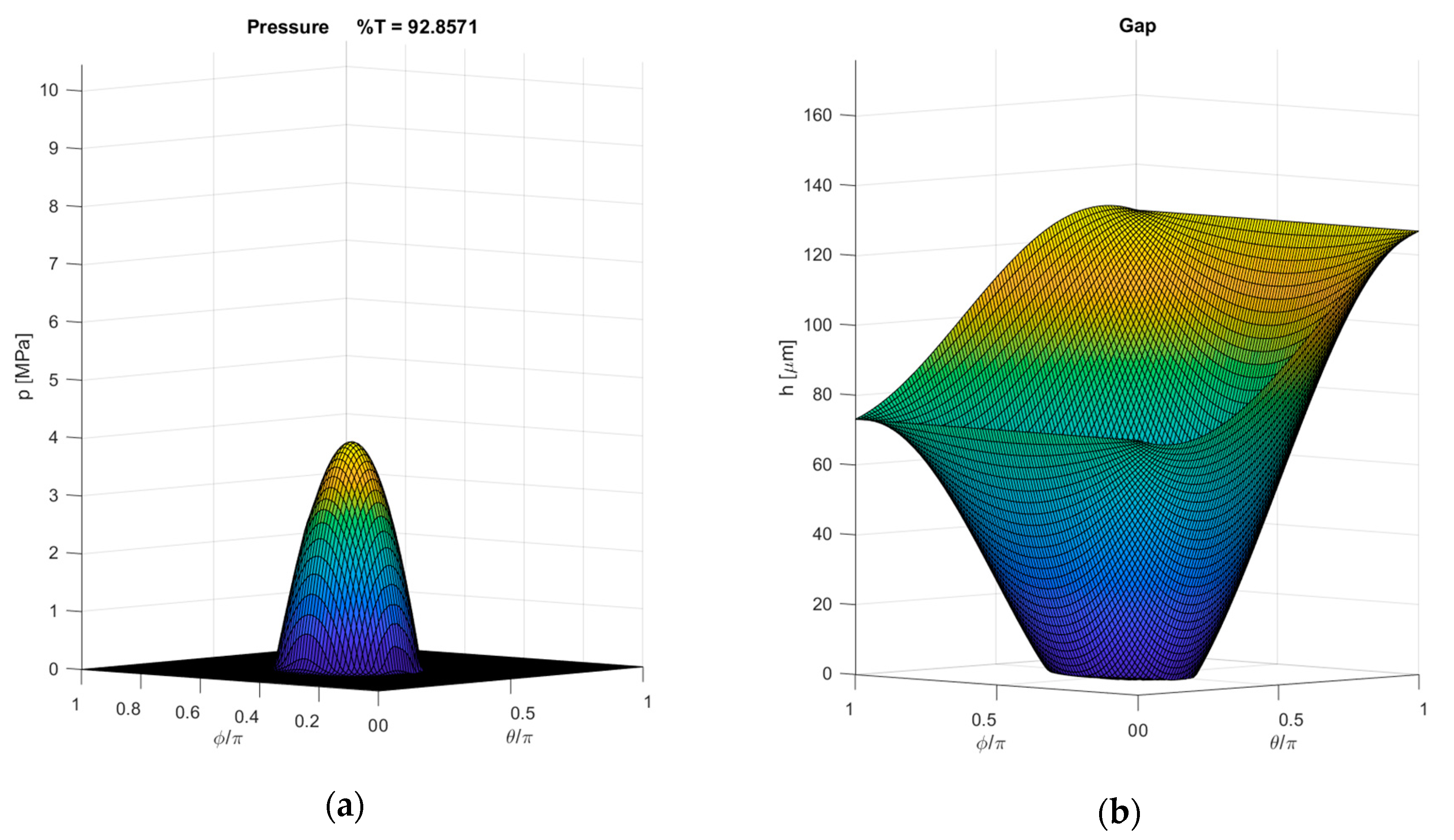
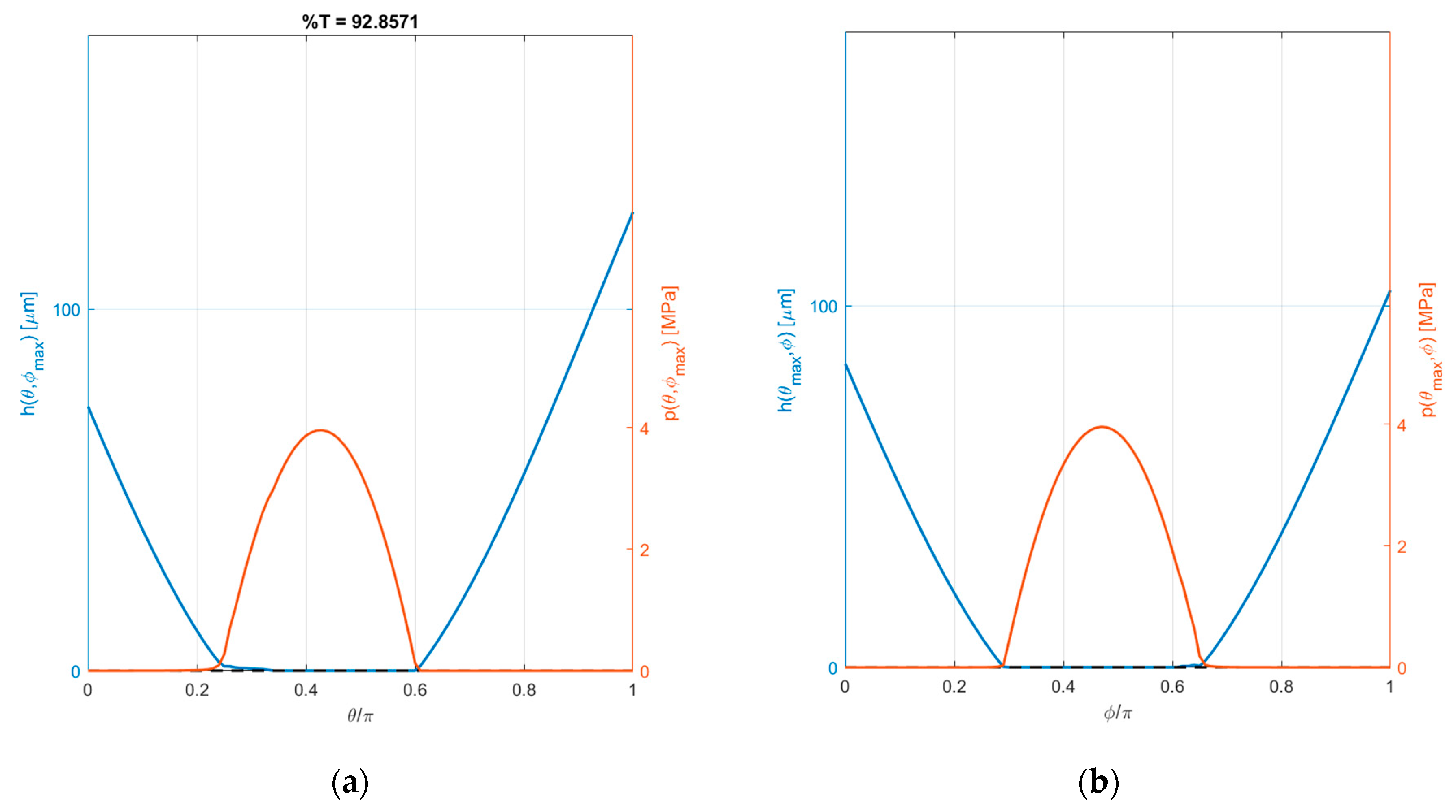
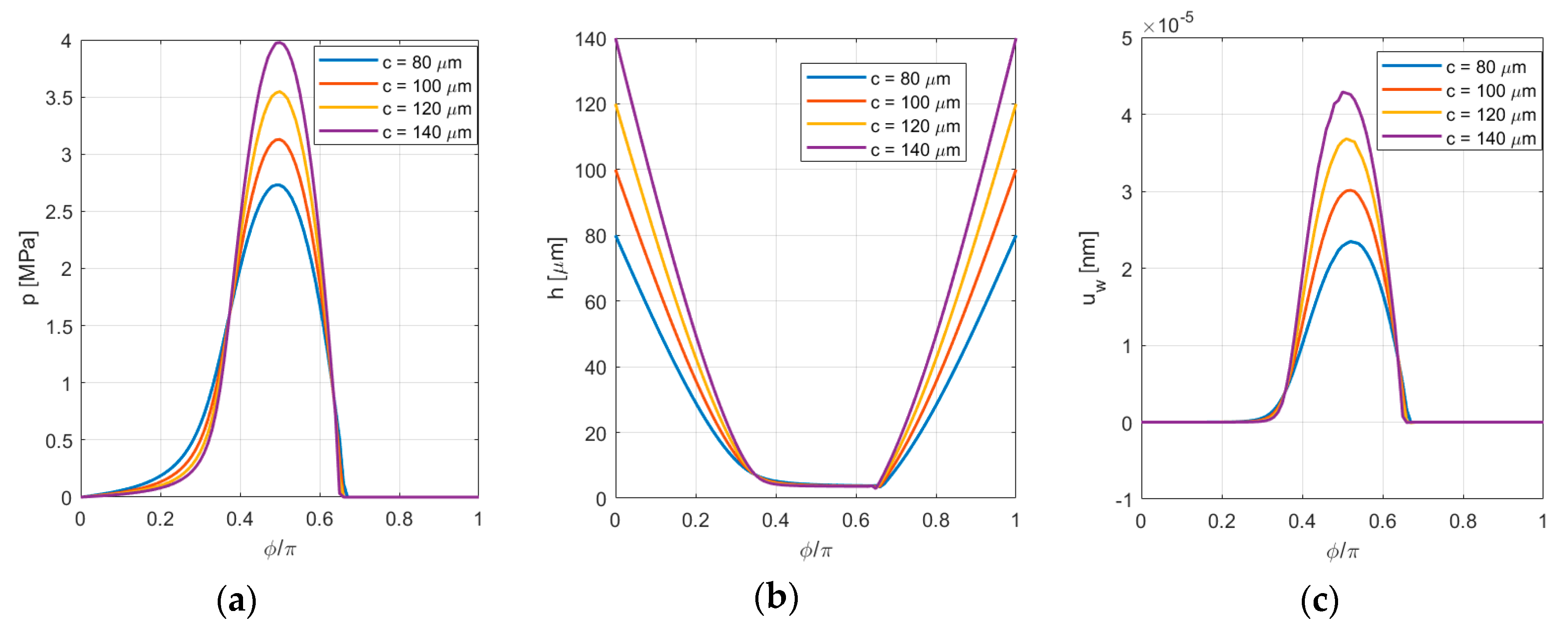
- The simulation conducted in the framework of the radial clearance sensitivity analysis showed the expected tribological behavior in terms of classical EHL shapes.
- -
- Build a finite element model to calculate the deformation field of both acetabular cup and femoral head, in order to analyze the tribological behavior of other types of THRs in which both contact bodies must be considered deformable;
- -
- Consider the surfaces’ topography in the gap calculation in order to analyze a more realistic surface in the mixed lubrication mode and also to consider material transfer phenomena;
- -
- Improve the wear modeling in order to consider more specific wear modes, such as, for example, delamination effects.
Supplementary Materials
Author Contributions
Funding
Conflicts of Interest
Nomenclature
| FE, AA, IER | Flexion–Extension, Adduction–Abduction, Internal–External Rotation |
| ML, AP, PD | Medio–Lateral, Anterior–Posterior, Proximo–Distal hip axes |
| , , | Cartesian axes |
| Load vector | |
| Angular velocity vector | |
| , | Acetabular cup inclination angle and anteversion angle |
| Rotation matrix for a rotation around the axis | |
| Rotation matrix from the hip reference frame to the cup one | |
| Fluid pressure | |
| Fluid film thickness | |
| Fluid density | |
| Nominal fluid density | |
| , | Dowson–Higginson coefficients |
| Fluid viscosity | |
| Effective nominal viscosity | |
| Barus exponential coefficient | |
| , | Cross viscosities in correspondence of and theoretically shear rate |
| , | Cross viscosity model parameters |
| Average shear rate | |
| Geometrical gap | |
| Total surfaces’ deformation | |
| , | Deformation due to fluid pressure and contact deformation |
| Linear wear | |
| Boundary layer thickness | |
| Contact pressure | |
| Total pressure | |
| Wear rate | |
| , | Wear factor function and nominal wear factor |
| Modified Archard model exponential coefficient | |
| Average roughness | |
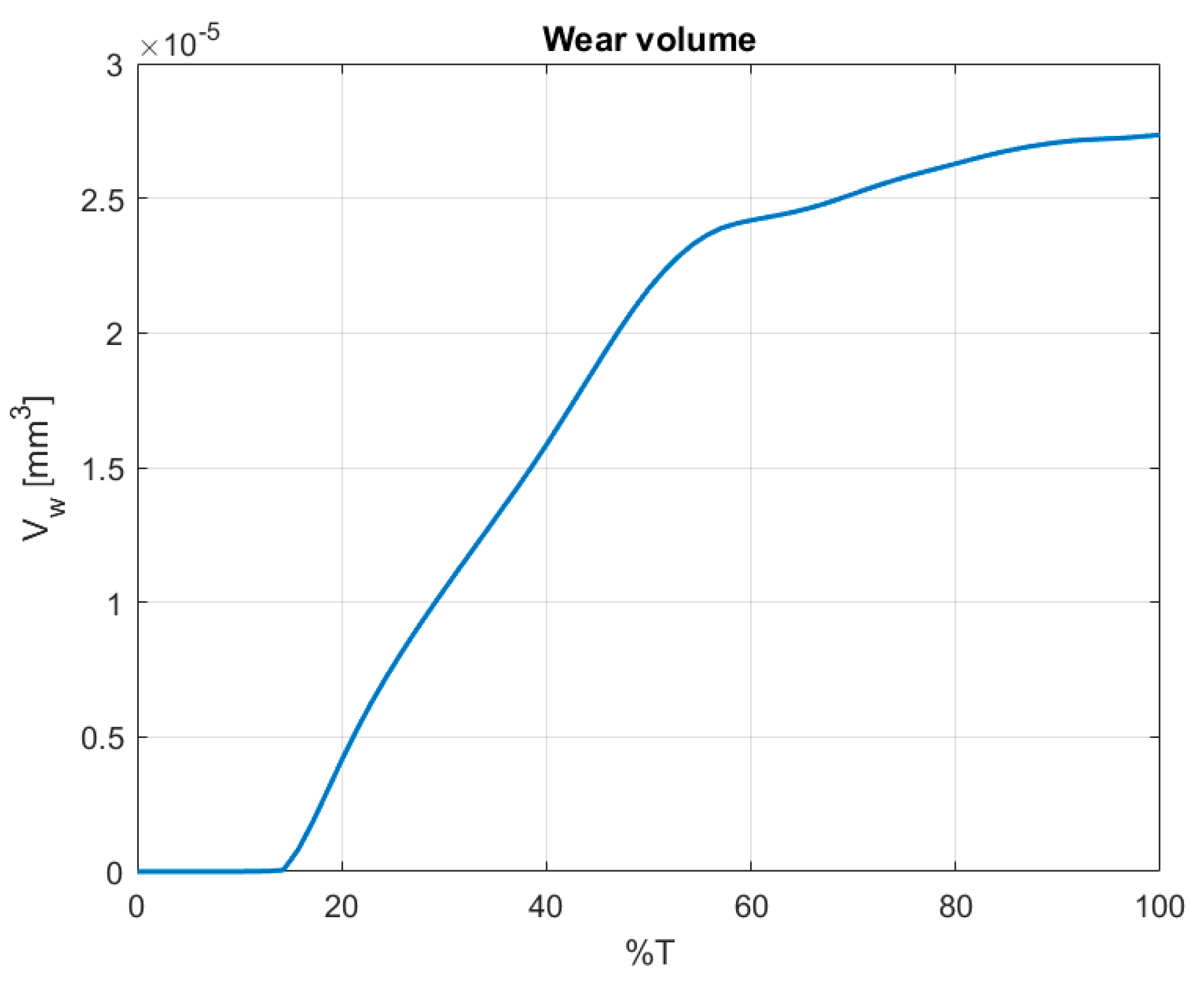
| Wear volume | |
| , | Spherical angles |
| Time | |
| Radial unit vector | |
| , | Femoral head and acetabular cup radii |
| Radial clearance | |
| Acetabular cup thickness | |
| , | Acetabular cup Young modulus and Poisson coefficient |
| Constraint column model constant | |
| Boundary pressure | |
| , | Eccentricity vector and its dimensionless form |
| , | Entraining and sliding velocity vectors |
| Spherical rotation matrix | |
| , , | Finite difference subscripts |
| Discretized pressure vector | |
| , | Discretized Reynolds equation vector and its analytical Jacobian matrix |
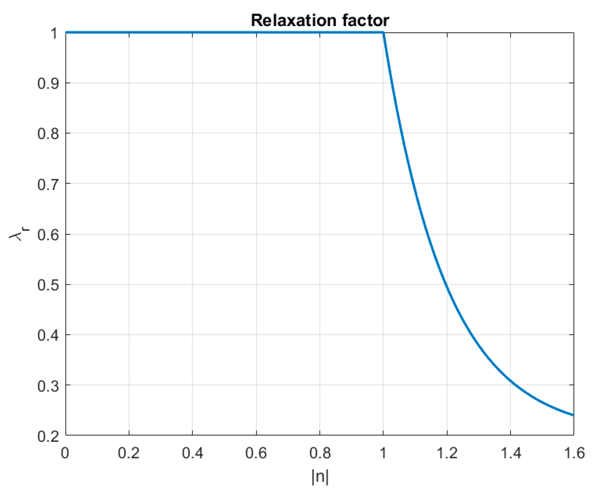
| , , | Relaxation factor and its parameters |
| , | Iterative cycles residual and tolerance |
| , | Load difference function vector and its numerical Jacobian matrix |
| Volumetric wear rate |
References
- Pramanik, S.; Agarwal, A.K.; Rai, K. Chronology of total hip joint replacement and materials development. Trends Biomater. Artif. Organs 2005, 19, 15–26. [Google Scholar]
- Carr, A.J.; Robertsson, O.; Graves, S.; Price, A.J.; Arden, N.K.; Judge, A.; Beard, D.J. Knee replacement. Lancet 2012, 379, 1331–1340. [Google Scholar] [CrossRef]
- Jin, Z.; Yonggang, M.; Yuanzhong, H.; Jianbin, L. In Memoriam: Duncan Dowson (1928–2020). Friction 2020, 8, 1–3. [Google Scholar] [CrossRef] [Green Version]
- Fisher, J.; Dowson, D. Tribology of total artificial joints. Proc. Inst. Mech. Eng. Part H J. Eng. Med. 1991, 205, 73–79. [Google Scholar] [CrossRef]
- Ruggiero, A.; Sicilia, A. Lubrication modeling and wear calculation in artificial hip joint during the gait. Tribol. Int. 2020, 142, 105993. [Google Scholar] [CrossRef]
- Wang, F.; Wang, L.; Sun, M. Tribological modelling of spherical bearings with complex spherical-based geometry and motion. WIT Trans. Eng. Sci. 2010, 66, 3–15. [Google Scholar]
- Harun, M.; Wang, F.; Jin, Z.; Fisher, J. Long-term contact-coupled wear prediction for metal-on-metal total hip joint replacement. Proc. Inst. Mech. Eng. Part J J. Eng. Tribol. 2009, 223, 993–1001. [Google Scholar] [CrossRef]
- Dumbleton, J.H. Tribology of Natural and Artificial Joints; Elsevier: Amsterdam, The Netherlands, 1981. [Google Scholar]
- Nordin, M.; Frankel, V.H. Basic Biomechanics of the Musculoskeletal System; Lippincott Williams & Wilkins: Philadelphia, PA, USA, 2001. [Google Scholar]
- Mattei, L.; di Puccio, F.; Piccigallo, B.; Ciulli, E. Lubrication and wear modelling of artificial hip joints: A review. Tribol. Int. 2011, 44, 532–549. [Google Scholar] [CrossRef]
- Zivic, F.; Affatato, S.; Trajanovic, M.; Schnabelrauch, M.; Grujovic, N.; Choy, K.L. Biomaterials in Clinical Practice: Advances in Clinical Research and Medical Devices; Springer: Berlin, Germany, 2017. [Google Scholar]
- Affatato, S.; Ruggiero, A.; Merola, M. Advanced biomaterials in hip joint arthroplasty. A review on polymer and ceramics composites as alternative bearings. Compos. Part B Eng. 2015, 83, 276–283. [Google Scholar] [CrossRef]
- Merola, M.; Affatato, S. Materials for hip prostheses: A review of wear and loading considerations. Materials 2019, 12, 495. [Google Scholar] [CrossRef] [Green Version]
- Aherwar, A.; Singh, A.K.; Patnaik, A. Current and future biocompatibility aspects of biomaterials for hip prosthesis. AIMS Bioeng. 2015, 3, 23–43. [Google Scholar] [CrossRef]
- Jalali-Vahid, D.; Jagatia, M.; Jin, Z.; Dowson, D. Prediction of lubricating film thickness in a ball-in-socket model with a soft lining representing human natural and artificial hip joints. Proc. Inst. Mech. Eng. Part J J. Eng. Tribol. 2001, 215, 363–372. [Google Scholar] [CrossRef]
- Wang, F.; Jin, Z. Prediction of elastic deformation of acetabular cups and femoral heads for lubrication analysis of artificial hip joints. Proc. Inst. Mech. Eng. Part J J. Eng. Tribol. 2004, 218, 201–209. [Google Scholar] [CrossRef]
- Jalali-Vahid, D.; Jin, Z.; Dowson, D. Elastohydrodynamic lubrication analysis of hip implants with ultra high molecular weight polyethylene cups under transient conditions. Proc. Inst. Mech. Eng. Part C J. Mech. Eng. Sci. 2003, 217, 767–777. [Google Scholar] [CrossRef]
- Wang, F.; Jin, Z. Lubrication modelling of artificial hip joints: From fluid film to boundary lubrication regimes. In Proceedings of the Engineering Systems Design and Analysis, Manchester, UK, 19–22 July 2004; pp. 605–611. [Google Scholar]
- Wang, F.; Brockett, C.; Williams, S.; Udofia, I.; Fisher, J.; Jin, Z. Lubrication and friction prediction in metal-on-metal hip implants. Phys. Med. Biol. 2008, 53, 1277. [Google Scholar] [CrossRef]
- Zhu, D.; Hu, Y.-Z. The study of transition from elastohydrodynamic to mixed and boundary lubrication. STLE/ASME HS Cheng Tribol. Surveill 1999, 150–156. [Google Scholar]
- Zhu, D. On some aspects of numerical solutions of thin-film and mixed elastohydrodynamic lubrication. Proc. Inst. Mech. Eng. Part J J. Eng. Tribol. 2007, 221, 561–579. [Google Scholar] [CrossRef]
- Gao, L.; Wang, F.; Yang, P.; Jin, Z. Effect of 3D physiological loading and motion on elastohydrodynamic lubrication of metal-on-metal total hip replacements. Med. Eng. Phys. 2009, 31, 720–729. [Google Scholar] [CrossRef]
- Jin, Z.; Dowson, D. A full numerical analysis of hydrodynamic lubrication in artificial hip joint replacements constructed from hard materials. Proc. Inst. Mech. Eng. Part C J. Mech. Eng. Sci. 1999, 213, 355–370. [Google Scholar] [CrossRef]
- Askari, E.; Andersen, M. A modification on velocity terms of Reynolds equation in a spherical coordinate system. Tribol. Int. 2019, 131, 15–23. [Google Scholar] [CrossRef] [Green Version]
- Jalali-Vahid, D.; Jagatia, M.; Jin, Z.; Dowson, D. Prediction of lubricating film thickness in UHMWPE hip joint replacements. J. Biomech. 2001, 34, 261–266. [Google Scholar] [CrossRef]
- Jalali-Vahid, D.; Jin, Z. Transient elastohydrodynamic lubrication analysis of ultra-high molecular weight polyethylene hip joint replacements. Proc. Inst. Mech. Eng. Part C J. Mech. Eng. Sci. 2001, 216, 409–420. [Google Scholar] [CrossRef]
- Udofia, I.; Jin, Z. Elastohydrodynamic lubrication analysis of metal-on-metal hip-resurfacing prostheses. J. Biomech. 2003, 36, 537–544. [Google Scholar] [CrossRef]
- Wang, F.; Jin, Z. Transient elastohydrodynamic lubrication of hip joint implants. J. Tribol. 2008, 130, 011007. [Google Scholar] [CrossRef]
- Kharb, A.; Saini, V.; Jain, Y.; Dhiman, S. A review of gait cycle and its parameters. IJCEM Int. J. Comput. Eng. Manag. 2011, 13, 78–83. [Google Scholar]
- Bergmann, G.; Bender, A.; Dymke, J.; Duda, G.; Damm, P. Standardized loads acting in hip implants. PLoS ONE 2016, 11, e0155612. [Google Scholar] [CrossRef]
- van Leeuwen, H. The determination of the pressure–viscosity coefficient of a lubricant through an accurate film thickness formula and accurate film thickness measurements. Proc. Inst. Mech. Eng. Part J J. Eng. Tribol. 2009, 223, 1143–1163. [Google Scholar] [CrossRef] [Green Version]
- Gao, L.; Dowson, D.; Hewson, R.W. A numerical study of non-Newtonian transient elastohydrodynamic lubrication of metal-on-metal hip prostheses. Tribol. Int. 2016, 93, 486–494. [Google Scholar] [CrossRef] [Green Version]
- Archard, J.; Hirst, W. The wear of metals under unlubricated conditions. Proc. R. Soc. Lond. Ser. A Math. Phys. Sci. 1956, 236, 397–410. [Google Scholar]
- Gao, L.; Dowson, D.; Hewson, R.W. Predictive wear modeling of the articulating metal-on-metal hip replacements. J. Biomed. Mater. Res. Part B Appl. Biomater. 2017, 105, 497–506. [Google Scholar] [CrossRef]
- Gao, L.; Hua, Z.; Hewson, R.; Andersen, M.S.; Jin, Z. Elastohydrodynamic lubrication and wear modelling of the knee joint replacements with surface topography. Biosurface Biotribol. 2018, 4, 18–23. [Google Scholar] [CrossRef]
- Jagatia, M.; Jin, Z. Elastohydrodynamic lubrication analysis of metal-on-metal hip prostheses under steady state entraining motion. Proc. Inst. Mech. Eng. Part H J. Eng. Med. 2001, 215, 531–541. [Google Scholar] [CrossRef] [PubMed]
- Yan, Y.; Neville, A.; Dowson, D. Biotribocorrosion—An appraisal of the time dependence of wear and corrosion interactions: I. The role of corrosion. J. Phys. D Appl. Phys. 2006, 39, 3200. [Google Scholar] [CrossRef]
- di Puccio, F.; Mattei, L. Biotribology of artificial hip joints. World J. Orthop. 2015, 6, 77. [Google Scholar] [CrossRef] [PubMed]
- Mattei, L.; di Puccio, F.; Ciulli, E. A comparative study of wear laws for soft-on-hard hip implants using a mathematical wear model. Tribol. Int. 2013, 63, 66–77. [Google Scholar] [CrossRef]
- Bergiers, S.; Hothi, H.; Richards, R.; Henckel, J.; Hart, A. Quantifying the bearing surface wear of retrieved hip replacements. Biosurface Biotribol. 2019, 5, 28–33. [Google Scholar] [CrossRef]


| Parameter | Value |
|---|---|
| Acetabular cup inclination angle | [10] |
| Acetabular cup anteversion angle | |
| Femoral head radius | [10] |
| Radial clearance | [10] |
| Acetabular cup thickness | [15] |
| Acetabular cup Young modulus | [10] |
| Acetabular cup Poisson ratio | [10] |
| Barus model exponential factor | [31] |
| Cross model upper limit viscosity | [32] |
| Cross model lower limit viscosity | [32] |
| Cross model parameter | [32] |
| Cross model parameter | [32] |
| Synovial fluid nominal density | |
| Density model parameter | [31] |
| Density model parameter | [31] |
| Boundary pressure | |
| Boundary layer thickness | [19,35] |
| Roughness | [10] |
| Nominal wear factor | [10] |
| Archard model exponential factor | [34] |
| Spherical domain mesh density | |
| Time domain steps number | |
| Pressure tolerance | |
| Load tolerance | |
| Relaxation parameter | |
| Relaxation parameter | |
| Increment for the numerical Jacobian |
© 2020 by the authors. Licensee MDPI, Basel, Switzerland. This article is an open access article distributed under the terms and conditions of the Creative Commons Attribution (CC BY) license (http://creativecommons.org/licenses/by/4.0/).
Share and Cite
Ruggiero, A.; Sicilia, A. A Mixed Elasto-Hydrodynamic Lubrication Model for Wear Calculation in Artificial Hip Joints. Lubricants 2020, 8, 72. https://doi.org/10.3390/lubricants8070072
Ruggiero A, Sicilia A. A Mixed Elasto-Hydrodynamic Lubrication Model for Wear Calculation in Artificial Hip Joints. Lubricants. 2020; 8(7):72. https://doi.org/10.3390/lubricants8070072
Chicago/Turabian StyleRuggiero, Alessandro, and Alessandro Sicilia. 2020. "A Mixed Elasto-Hydrodynamic Lubrication Model for Wear Calculation in Artificial Hip Joints" Lubricants 8, no. 7: 72. https://doi.org/10.3390/lubricants8070072
APA StyleRuggiero, A., & Sicilia, A. (2020). A Mixed Elasto-Hydrodynamic Lubrication Model for Wear Calculation in Artificial Hip Joints. Lubricants, 8(7), 72. https://doi.org/10.3390/lubricants8070072