Article

Evaluation of Transient Response of Turbochargers and Turbines Using Database Method for the Nonlinear Forces of Journal Bearings

by
Athanasios Chasalevris
1,* and
Jean-Charles Louis
2
1
School of Mechanical Engineering, National Technical University of Athens, 15780 Athens, Greece
2
SeaTech, Ecole d’ingénieurs - Université de Toulon, CS 60584 - 83041 Toulon, France
*
Author to whom correspondence should be addressed.
Lubricants 2019, 7(9), 78; https://doi.org/10.3390/lubricants7090078
Submission received: 12 July 2019 / Revised: 21 August 2019 / Accepted: 28 August 2019 / Published: 3 September 2019
(This article belongs to the Special Issue Fluid-Film Lubrication II)

Abstract

:
The paper extents the fluid film bearing database method to arbitrary fixed bearing profiles including floating ring bearings. The method is applied to evaluate rotordynamic response of an automotive turbocharger, modeled as rigid rotor, and of a turbine-generator shaft train for power generation modeled as flexible rotor through the transient transfer matrix method. The methodology claims to render drastically faster evaluation of transient response of rotating systems with nonlinear bearings regardless the complexity of the bearing models implemented. The computational time of transient response is similar to this when short bearing expressions are used. Turbocharger rotordynamic simulation considers the use of nonlinear bearing models as mandatory, and several case studies have to be performed for the definition of key design parameters of floating ring bearings. The bearing database method offers the tool for a severe total time reduction in rotordynamic calculations, with the possibility to implement advanced thermohydrodynamic bearing models to the rotordynamic algorithm as fast as short bearing approximation formulas. Furthermore, the rotordynamic design of large turbine shaft trains is still based on linear harmonic analysis which leads to conservative designs. The database method aims to include the transient response of nonlinear rotor models as a standard procedure in the rotordynamic design of large shaft trains, which nowadays is avoided due to high time cost and complexity.

1. Introduction

In rotor bearing systems of medium and high speed, the fluid film bearing forces have to be solved at every discrete time step of the integration of system equations when nonlinear transient response is evaluated. This requires considerable evaluation time spent on bearing subroutines of the rotordynamic algorithm. The evaluation time is a very important matter in rotordynamic design tools as the engineer should be able to try geometrical and physical properties conveniently, in terms of time required to get results for unbalance response and other standard calculations. It is a fact that the accurate and relatively fast analytical models of finite length journal bearing forces are still cumbersome and available only for simple bearing profiles [1,2]. Furthermore, despite the computational capacity of computers, the numerical bearing models may still require a considerable evaluation time for an entire rotor run-up. The database methods have been proposed in 1993 for fixed bearing profile to overcome the above shortcomings [3,4,5,6,7,8,9]. Similar approaches had been already used since the 60′s. Notable are mobility maps introduced by Booker in 1965 [10,11] and the impedance method introduced by Childs et al. in 1977 [12].
For all rotor systems supported by fluid film bearings, the linear stability assessment which implements linear bearing stiffness and damping properties, the well-known 8 matrix elements, is not able to predict response at speeds higher than the instability threshold. Further to that, and probably of higher importance, is the fact that the linear theory where linear bearing properties and linear stability assessment are used, cannot predict that originally stable systems may go unstable when a sudden external excitation is applied. For these major reasons, the nonlinear stability study of slender rotor systems attracts increased attention.
The most popular way to implement nonlinear fluid film forces into a rotordynamic algorithm is the direct solution of the Reynolds equation [13,14,15], the approximate short and long bearing theory [13,14,15], and the use of higher order stiffness and damping coefficients [13,14,15]. Millions of integration steps may be required to evaluate a transient rotor-bearing response and the Reynolds equation has to be solved in each of these time intervals. Supposing a multi-bearing shaft train, the Reynolds equation should be solved for each bearing. Even for a high speed turbocharger rotor mounted on floating ring bearings, the Reynolds equation should be solved four times at each discrete time interval of the transient response, for the two bearings, and two films at each bearing. The approximate methods are very fast, but their accuracy is not applicable in common bearing profiles e.g., of industrial turbines, as their length to diameter ratio neither corresponds to a short nor a long bearing.
The database technique developed initially in [3], puts forward a fast and accurate implementation of fluid film forces in rotordynamic algorithms. Application of the method on simple bearing profiles and Jeffcott rotor has proved that the method not only had practically the same accuracy as the direct solving method, but also reduced dramatically the computation time of transient response. Recently, the method was applied in grooved floating ring bearings [7] where it was shown that transient response of turbochargers with simple circular floating rings can be evaluated in such a low time so to enable different considerations on the design optimization of such systems. Bearing database method has been also applied on rod fastening rotors with tilting pad bearings [8] where nonlinear phenomena where efficiently captured.
The key to apply the database technique is on the transformation of the Reynolds equation kinematic parameters, varying theoretically from −∞ to ∞, these being the velocity of the journal in two directions, to the variation on a finite range e.g., from −1 to 1. This is described in this paper for the representative case of a fixed lobe bearing of complex geometry for industrial applications in different way than what presented before [3,4,5,6,7,8,9]. The difference is that 4 parameters are considered in the database, enabling the calculation of oil film forces for a flow on a theoretically arbitrary profile. The key benefit of the current approach is that the database may consider the position of the journal attitude angle with respect to the bearing profile configuration, e.g., scallops, when talking for a fixed profile bearing. Furthermore, with the current approach, the database can be established for the case of floating ring bearings where the floating ring includes radial holes for the flow of oil between inner and outer film, and axial grooves as well. In the current paper, fixed lobe bearing profiles and floating ring bearings are considered.
Another benefit of the database method is that a very precise journal bearing model can be considered, including e.g., evaluation using edge commercial tools on THD lubrication principles. Parallel processing can be applied for the a priori to the rotordynamic analysis creation of the database with respect to the 4 parameter variation within finite range intervals which define a sparse or dense grid. However, in this paper, a Finite Difference Method (FDM) is used to evaluate the lubricant pressure depending on the four parameters of the database, without the type of the numerical solution to be restrictive for the applicability of the method. Using the database method, a very precise prediction of the bearing performance, e.g., using CFD, can be implemented in a rotordynamic algorithm as fast as a simple solution, e.g., short bearing approximation.
The paper considers two rotordynamic design applications of the database method. The extended database method is developed for simple floating ring bearing models [16] and it is applied to a simple high-speed system of an automotive turbocharger, considering rigid rotor [17]. The evaluation time for a rotor run-up and the respective optimization problem described in the paper is drastically reduced when Database Method is applied. The application of the database method in a turbine shaft train consisting of 3 rotors connected with rigid couplings. Four oil film bearings with complex profile are included [18]. When two bearings have equal dimensionless geometric parameters, e.g., length to diameter ratio and clearance to radius ratio, the oil film forces can be deducted from the same database. This instruction is explained in the paper. However, if a dimensional geometrical or physical parameter is different, e.g., dynamic viscosity, then different databases are needed, one for each dynamic viscosity value. The rotors are modeled using the Transient Transfer Matrix Method (TTMM) [19], explained in the Appendix B, and the bearings are modeled using the FDM with the Gumbel’s boundary condition applying [13]. The model includes flexible bearing pedestals as lumped mass models on linear springs and dampers [18].
Depending on the type of machine and the rotordynamic problem, the bearing database method can reduce the evaluation time of the entire rotordynamic algorithm at a similar level; this happens for systems with few degrees of freedom, e.g., a rigid rotor mounted on floating ring bearings—simulation of a turbocharger. Depending on the time consumption of the bearing subroutine with respect to the overall calculations, the database method renders a corresponding reduction of the total evaluation time.

2. The Database Method and Its Application in Journal Bearings

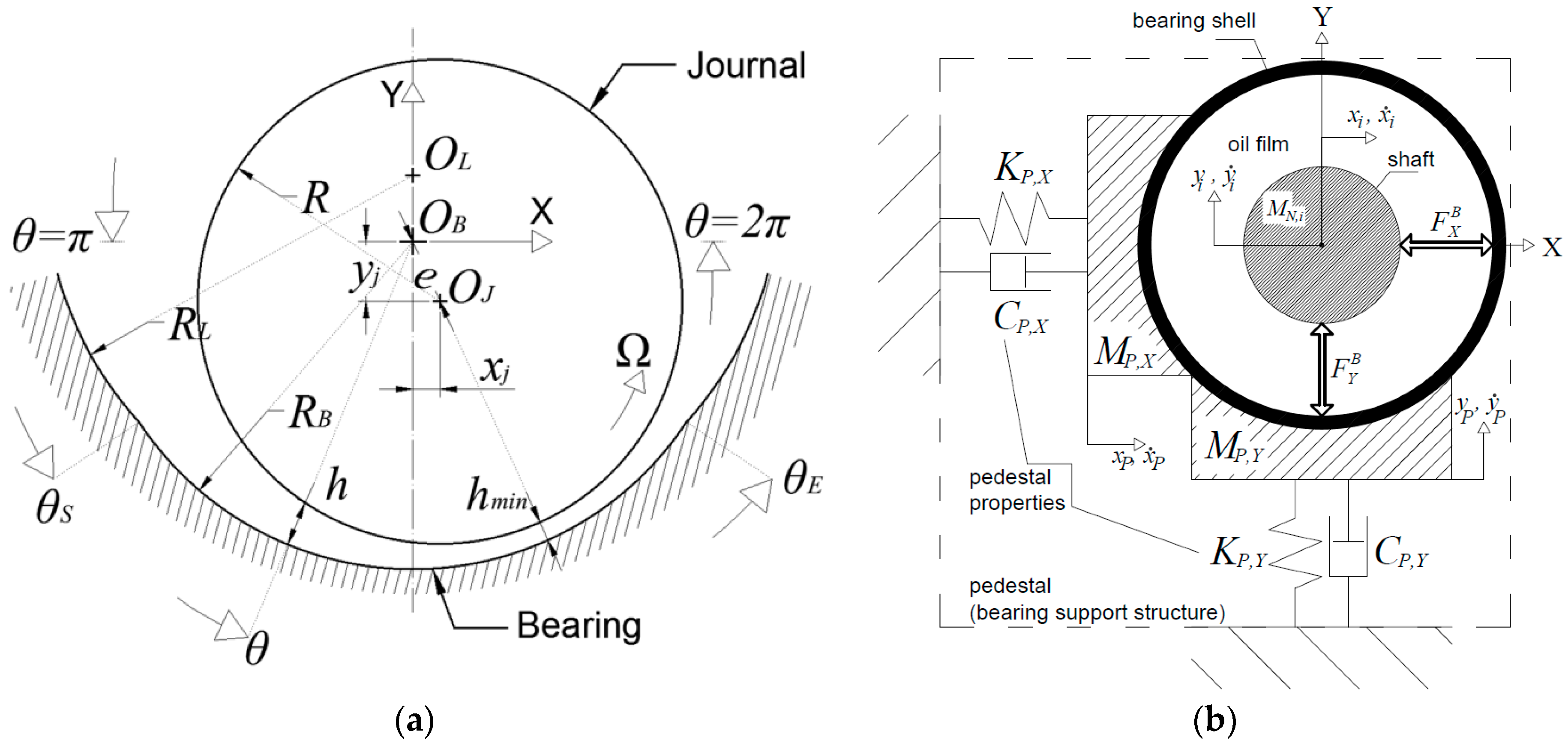
2.1. Application of the Method in Fixed Profile Bearings

A journal bearing of fixed geometry is represented in Figure 1a. As a matter of generality, the bearing consists of two circular sectors: (a) A concentric to the bearing center O B ( x B , y B ) circular sector of radius R B for θ S < θ < θ Ε , and (b) a circular sector of radius R L , for θ < θ S or θ > θ Ε , centered at O L ( x L , y L ) . The latter sector is a preloaded lobe, called also preloaded pad, as its center does not coincide to the bearing center. Such a geometric configuration increases the journal bearing effective eccentricity and this is the principle to enhanced bearing stability of preloaded bearings [15], known also as elliptical bearings or lobe bearings. When the journal center O J ( x j , y j ) does not coincide to the bearing center O B , the eccentricity e = ( x j 2 + y j 2 ) 1 / 2 forms a fluid film thickness h between the sliding surfaces of the journal and the bearing, well approximated by the formulas in Equation (1), which can be expressed in dimensionless form as H = h / c B .
The bearing housing, called also bearing pedestal, see Figure 1b, is considered as a 2 DOF system with one lumped mass M P , X , M P , Y (pedestal mass) in vertical and in horizontal direction. The lumped pedestal masses are connected through linear springs of stiffness coefficient K P , X , K P , Y , and through linear dampers of damping coefficient C P , X , C P , Y , to the ground. The nonlinear fluid film impedance forces F X B and F Y B are functions of eight variables appearing explicitly in the equations of motion described in Appendices: the horizontal and vertical displacement of the journals x j , y j , and their respective time derivatives x ˙ j , y ˙ j , and the horizontal and vertical displacement of the pedestal x P , y P , and their respective time derivatives x ˙ P , y ˙ P . The rotating speed is also a parameter in equations of motion but it does not appear explicitly as it is a parameter in fluid film forces function.
In Equation (1), x B = y B = x L = 0 (see Figure 1a), while y L 0 ; c B = R B R is the bearing clearance, called also assembly clearance, and c P = R L R is the pad clearance (or machined pad clearance). It is clear that in Figure 1a, c P > c B and consequently R L >   R B , and thus the lobe sector is preloaded with a preload m = 1 c B / c P . Furthermore, the bearing has a length L B in Z direction, the lubricant is characterized by a dynamic viscosity μ which for simplicity is assumed constant in this paper as the flow of the lubricant is considered isoviscous, and the journal rotates around its center with rotating speed Ω, called spinning speed. Under dynamic conditions, the journal will perform whirling motion inside the bearing clearance, with velocities x ˙ j and y ˙ j .
h = { c B ( x j x B ) · cos ( θ ) ( y j y B ) · sin ( θ ) ,   θ S θ θ E c P ( x j x L ) · cos ( θ ) ( y j y L ) · sin ( θ ) ,   θ < θ S   or   θ > θ E
The lubrication problem which is the evaluation of lubricant pressure distribution inside the bearing clearance for laminar, isothermal, isoviscous flow is defined by the Reynolds equation which includes all the previously defined geometric and physical parameters, see Equation (2) [13].
1 μ R 2 θ ( h 3 p θ ) + h 3 μ 2 p z 2 = 6 Ω h θ + 12 d h d t
With the use of Equation (1), the right hand side (RHS) of Equation (2) is written after some math in Equation (3).
RHS = ( 6 Ω x j 12 y ˙ j ) sin θ ( 6 Ω y j + 12 x ˙ j )   cos θ    
Setting dimensionless variables in Equation (4), Equation (2) is written in Equation (5).
p ¯ = c B 2 p μ Ω R 2 ,   ε x = x j c B ,   ε y = y j c B ,   ε ˙ x = x ˙ j c B , ε ˙ y = y ˙ j c B ,   ε ¯ x ˙ = ε ˙ x Ω , ε ¯ y ˙ = ε ˙ y Ω ,   k = 2 R L ,   z ¯ = 2 z L ,   φ ˙ = x j y ˙ j y j x ˙ j ε x 2 + ε y 2
θ ( H 3 p ¯ θ ) + k 2 H 3 2 p ¯ z ¯ 2 = ( 6 ε x 12 ε ¯ y ˙ ) sin θ ( 6 ε y + 12 ε ¯ x ˙ )   cos θ
The problem on establishing a database for bearing performance directly from the Reynolds equation is that whereas the input parameters ε x and ε y may have values within the domain 1 < ε x , ε y < 1 , the input parameters ε ¯ x ˙ ,   ε ¯ y ˙ ( , ) cannot be defined within a specific domain. To overcome this problem, the Reynolds equation in the form of Equation (5) is divided by Q and then the Reynolds equation is written in Equation (6).
3 H 2 H θ p ¯ θ + H 3 2 p ¯ θ 2 + k 2 H 3 2 p ¯ z ¯ 2 = 6 x ¯ 1 sin θ 6 x ¯ 2 cos θ
The portion Q has two definitions:
  • If | ε x 2 ε ¯ y ˙ | > | ε y + 2 ε ¯ x ˙ | , then Q   =   |   ( ε x 2 ε ¯ ˙ y ) ( ε 2 Ω 2 ε x ε ¯ ˙ y + 2 ε y ε ¯ ˙ x ) ε ( ε x Ω 2 ε ¯ ˙ y ) |
  • If | ε x 2 ε ¯ y ˙ | < | ε y + 2 ε ¯ x ˙ | , then Q   =   |   ( ε y + 2 ε ¯ ˙ x ) ( ε 2 Ω 2 ε x ε ¯ ˙ y + 2 ε y ε ¯ ˙ x ) ε ( ε y Ω + 2 ε ¯ ˙ x ) |
The Reynolds equation in the form of Equation (6) has variables defined in Equations (7) and (8).
p ¯ = p ¯ Q ,   p ¯ θ = p ¯ θ ,       x ¯ 1 = ε x 2 ε ¯ ˙ y Q ,     x ¯ 2 = ε y + 2 ε ¯ ˙ x Q
H θ = H θ = ε x sin θ ε y cos θ
Practically, it is not possible to have Q   = 0 . This would correspond to a static case of a journal with zero eccentricity. At this theoretical case the lubrication problem would require a model of Couette flow. Furthermore, the case where | ε x 2 ε ¯ y ˙ | = | ε y + 2 ε ¯ x ˙ | is not a practical case. This may happen only when the accuracy of the computer is very low; not the case nowadays. The Reynolds Equation (6) can be solved after the four variables x ¯ 1 , x ¯ 2 , ε x , ε y are defined in the domain (−1,1). The solution can be a numerical solution scheme e.g., Finite Difference Method (FDM). Supposing that the FDM is implemented, with a definition of finite difference grid as N z × N θ , the respective intervals are defined as Δ z = L B / N z and Δ θ = ( θ Ε θ S ) / N θ . The angles θ S and θ E can be any angles on the circumference if the corresponding fluid film functions have been defined. The fact that x ¯ 1 , x ¯ 2 receive values in the domain (−1,1) finds its explanation in the limits of the functions which define x ¯ 1 , x ¯ 2 , see Equation (7), when eccentricity of the journal approaches 1, or journal velocity approaches infinity (only a theoretical case).
  • If Q > 0 , then the resulting fluid film forces and torque components are given in dimensionless form in Equation (9):
    { F ¯ x + F ¯ y + T ¯ 1 T ¯ 2 + } = { i = 1 N z j = 1 N θ ( Δ θ · p ¯ i , j · cos θ j ) i = 1 N z j = 1 N θ ( Δ θ · p ¯ i , j · sin θ j ) i = 1 N z j = 1 N θ ( Δ θ H θ , j ) i = 1 N z j = 1 N θ ( Δ θ · p ¯ θ i , j · H j ) }
    For Gümbel boundary conditions, only p ¯ i , j > 0 values are implemented in the double sum.
  • If Q < 0 , then the resulting fluid film forces and friction torque components are given in dimensionless form in Equation (10):
    { F ¯ x F ¯ y T ¯ 1 T ¯ 2 } = { i = 1 N z j = 1 N θ ( Δ θ · p ¯ i , j · cos θ j ) i = 1 N z j = 1 N θ ( Δ θ · p ¯ i , j · sin θ j ) i = 1 N z j = 1 N θ ( Δ θ H θ , j ) i = 1 N z j = 1 N θ ( Δ θ · p ¯ θ i , j · H j ) }
    For Gümbel boundary conditions, only p ¯ i , j < 0 values are implemented in the double sum.
In both cases (1) and (2) the resulting fluid film forces and friction torque in dimensional form are defined in Equation (11).
{ F x F y T } = μ L B Ω R 3 N z c B 2 Q { F ¯ x F ¯ y c B T ¯ 1 Q + 1 2 c B T ¯ 2 }
The bearing forces and torques database dat can be then constructed in Equation (12) where variables ε x and ε y vary from −0.9 to 0.9 within INT = 100 intervals, while variables x ¯ 1 and x ¯ 2 vary from −0.99 to 0.99 within INT = 100 intervals. Further columns can be added in the database corresponding to further outputs like e.g., rising temperature when THD model is implemented. The number of INT = 100 intervals can be sufficient to create a database that corresponds well in the demands for bearing forces under mild dynamic conditions, which means relatively low response around equilibrium. However, parallel processing can offer higher number of intervals, e.g., 400 or even 600, with the number of intervals to be different for each variable. It makes sense the database dat to include combinations of ε x and ε y such that they render ε = ( ε x 2 + ε y 2 ) 1 / 2 < 1 only.
For the use of the database in a rotordynamic algorithm for transient response analysis a 4-D interpolation should be implemented. The interpolation scheme can be linear or of higher order. The linear 4-D interpolation is presented hereby and the results following in the next sections depict its efficiency.
For i, j, k, m from 1 to INT
d a t ( i , j , k , m , 1 ) = F ¯ y + ( ε x , i ,   ε y , j ,   x ¯ 1 , k ,   x ¯ 2 , m ) d a t ( i , j , k , m , 2 ) = F ¯ x + ( ε x , i ,   ε y , j ,   x ¯ 1 , k ,   x ¯ 2 , m ) d a t ( i , j , k , m , 3 ) = F ¯ y ( ε x , i ,   ε y , j ,   x ¯ 1 , k ,   x ¯ 2 , m )     d a t ( i , j , k , m , 4 ) = F ¯ x ( ε x , i ,   ε y , j ,   x ¯ 1 , k ,   x ¯ 2 , m ) d a t ( i , j , k , m , 5 ) = T ¯ 1 ( ε x , i ,   ε y , j ,   x ¯ 1 , k ,   x ¯ 2 , m ) d a t ( i , j , k , m , 6 ) = T ¯ 2 + ( ε x , i ,   ε y , j ,   x ¯ 1 , k ,   x ¯ 2 , m ) d a t ( i , j , k , m , 7 ) = T ¯ 2 ( ε x , i ,   ε y , j ,   x ¯ 1 , k ,   x ¯ 2 , m )
next m, k, j, i.
At a discrete time moment of transient response, the bearing model requires at least 5 input variables in order to render the output forces and friction moments: the horizontal and vertical displacement of the journal x j and y j , their respective velocities x ˙ j and y ˙ j , and the rotating speed Ω. When the bearing support motion is included as a parameter in the algorithm, the journal bearing lubrication problem still requires five inputs: two relative displacements and two relative velocities of the journal with respect of the bearing, and the rotating speed. Supposing that a group of x j , y j , x ˙ j , y ˙ j , and Ω are rendered from the motion equations solver to the bearing subroutine at the time moment t 1 , then the four variables ε x , ε y , x ¯ 1 , and x ¯ 2 are computed from Equations (4) and (7), or (4) and (8). With INT to be the number of intervals for each variable as in Equation (12), then the index numbers a 2 ,   β 2 , γ 2 , δ 2 which are real numbers, used in the database in Equation (12) correspond to the actual values ε x , ε y , x ¯ 1 , x ¯ 2 defined in Equation (13). Then the side indexes are defined as a 1 ,   β 1 , γ 1 , δ 1 (integers) and a 0 ,   β 0 , γ 0 , δ 0 (integers) in Equation (13).
{ a 2 β 2 γ 2 δ 2 } = { ε x + 0.90 + 2 · 0.90 / ( INT 1 ) 2 · 0.90 / ( INT 1 ) ε y + 0.90 + 2 · 0.90 / ( INT 1 ) 2 · 0.90 / ( INT 1 ) x ¯ 1 + 0.99 + 2 · 0.99 / ( INT 1 ) 2 · 0.99 / ( INT 1 ) x ¯ 2 + 0.99 + 2 · 0.99 / ( INT 1 ) 2 · 0.99 / ( INT 1 ) } ,   { a 1 β 1 γ 1 δ 1 } = { ceil ( a 2 ) ceil ( β 2 ) ceil ( γ 2 ) ceil ( δ 2 ) } ,     { a 0 β 0 γ 0 δ 0 } = { a 1 1 β 1 1 γ 1 1 δ 1 1 }    
For a 4-D interpolation, 4 × 4 = 16 coefficients should be calculated in order to implement the interpolation of the given values in the database [20]. Furthermore, the sign of Q will indicate if the dimensionless fluid film forces and friction torque should be collected from the F ¯ x + , F ¯ y + , T ¯ 2 + values, or from the F ¯ x , F ¯ y , T ¯ 2 values. The T ¯ 1 value is independent from the sign of Q . The 16 coefficients are defined in Equation (14).
N 1 = ( a 1 a 2 ) ( β 1 β 2 ) ( γ 2 γ 0 ) ( δ 2 δ 0 ) ,   N 9 = ( a 1 a 2 ) ( β 1 β 2 ) ( γ 2 γ 0 ) ( δ 1 δ 2 ) N 2 = ( a 1 a 2 ) ( β 2 β 0 ) ( γ 2 γ 0 ) ( δ 2 δ 0 ) ,     N 10 = ( a 1 a 2 ) ( β 2 β 0 ) ( γ 2 γ 0 ) ( δ 1 δ 2 ) N 3 = ( a 2 a 0 ) ( β 1 β 2 ) ( γ 2 γ 0 ) ( δ 2 δ 0 ) ,     N 11 = ( a 2 a 0 ) ( β 1 β 2 ) ( γ 2 γ 0 ) ( δ 1 δ 2 ) N 4 = ( a 2 a 0 ) ( β 2 β 0 ) ( γ 2 γ 0 ) ( δ 2 δ 0 ) ,     N 12 = ( a 2 a 0 ) ( β 2 β 0 ) ( γ 2 γ 0 ) ( δ 1 δ 2 ) N 5 = ( a 1 a 2 ) ( β 1 β 2 ) ( γ 1 γ 2 ) ( δ 2 δ 0 ) ,     N 13 = ( a 1 a 2 ) ( β 1 β 2 ) ( γ 1 γ 2 ) ( δ 1 δ 2 ) N 6 = ( a 1 a 2 ) ( β 2 β 0 ) ( γ 1 γ 2 ) ( δ 2 δ 0 ) ,     N 14 = ( a 1 a 2 ) ( β 2 β 0 ) ( γ 1 γ 2 ) ( δ 1 δ 2 ) N 7 = ( a 2 a 0 ) ( β 1 β 2 ) ( γ 1 γ 2 ) ( δ 2 δ 0 ) ,     N 15 = ( a 2 a 0 ) ( β 1 β 2 ) ( γ 1 γ 2 ) ( δ 1 δ 2 ) N 8 = ( a 2 a 0 ) ( β 2 β 0 ) ( γ 2 γ 0 ) ( δ 2 δ 0 ) ,     N 16 = ( a 2 a 0 ) ( β 2 β 0 ) ( γ 1 γ 2 ) ( δ 1 δ 2 )
For the interpolation of F ¯ x , supposing that e.g., Q > 0 , 16 values of F ¯ x are picked from the database dat, corresponding to all combinations of the integer indexes evaluated in Equation (13), as in Equation (15).
F ¯ x , 1 = d a t ( a 0 , β 0 , γ 1 , δ 1 , 2 ) ,   F ¯ x , 5 = d a t ( a 0 , β 0 , γ 0 , δ 1 , 2 ) ,   F ¯ x , 9 = d a t ( a 0 , β 0 , γ 1 , δ 0 , 2 ) ,   F ¯ x , 13 = d a t ( a 0 , β 0 , γ 0 , δ 0 , 2 ) F ¯ x , 2 = d a t ( a 0 , β 1 , γ 1 , δ 1 , 2 ) ,   F ¯ x , 6 = d a t ( a 0 , β 1 , γ 0 , δ 1 , 2 ) ,   F ¯ x , 10 = d a t ( a 0 , β 1 , γ 1 , δ 0 , 2 ) ,   F ¯ x , 14 = d a t ( a 0 , β 1 , γ 0 , δ 0 , 2 ) F ¯ x , 3 = d a t ( a 1 , β 0 , γ 1 , δ 1 , 2 ) ,   F ¯ x , 7 = d a t ( a 1 , β 0 , γ 0 , δ 1 , 2 ) ,   F ¯ x , 11 = d a t ( a 1 , β 0 , γ 1 , δ 0 , 2 ) ,   F ¯ x , 15 = d a t ( a 1 , β 0 , γ 0 , δ 0 , 2 )   F ¯ x , 4 = d a t ( a 1 , β 1 , γ 1 , δ 1 , 2 ) ,   F ¯ x , 8 = d a t ( a 1 , β 1 , γ 0 , δ 1 , 2 ) ,   F ¯ x , 12 = d a t ( a 1 , β 1 , γ 1 , δ 0 , 2 ) ,     F ¯ x , 16 = d a t ( a 1 , β 1 , γ 0 , δ 0 , 2 )  
The interpolated values for F ¯ x , F ¯ y , T ¯ 1 , T ¯ 2 are then evaluated in Equation (16). For F ¯ y , i used in Equation (16), Equation (15) should be written for the values d a t ( , , , , 1 ) in advance. Similarly, T ¯ 1 and T ¯ 2 will be picked from the database elements d a t ( , , , , 5 ) and d a t ( , , , , 6 ) respectively.
F ¯ x = i = 1 16 N i F ¯ x , i   ,         F ¯ y = i = 1 16 N i F ¯ y , i     ,     T ¯ 1 = i = 1 16 N i T ¯ 1 , i       ,     T ¯ 2 = i = 1 16 N i T ¯ 2 , i
The benefit of the method is the evaluation time of bearing forces and friction torque, which is decreased up to approximately 100 times, without compromising accuracy. A Lagrange interpolation scheme can be also implemented. However, the forces will not obtain that different values compared to the linear interpolation, in order to raise concerns for the type of the interpolation method. Furthermore, the bearing forces included in the database can be calculated with enhanced bearing models such as thermohydrodynamic models (THD models) from any commercial software or other code. The reader should bear in mind that 4 variables is the minimum to describe the operating conditions of a non-circular bearing, e.g., lemon bore, 3-4 Lobe, offset halves, partial arc bearing. For the implementation of the method in floating ring bearings, 4 variables are still required if the floating ring includes holes for the flow of the lubricant from the outer to the inner film. At the case of plain circular floating ring bearing without holes in the ring, or at plain circular bearing, 3 variables are enough to create the database [3,7]. As a generic approach, if the bearing profile is always symmetric with respect to any attitude angle of the journal, then 3 variables are enough to create a database, this not being the case for the bearing of Figure 1a. Furthermore, the method can be applied in squeeze film dampers, and other bearing elements.

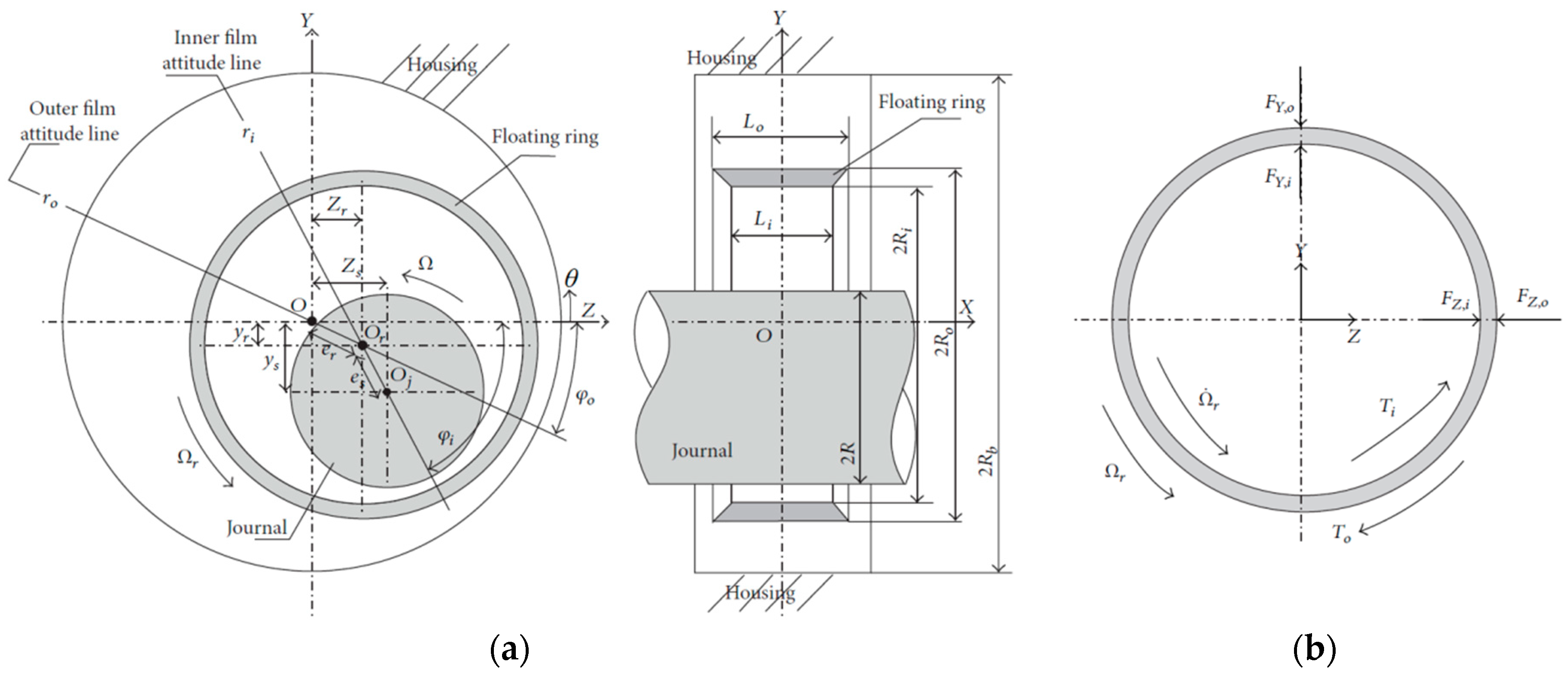
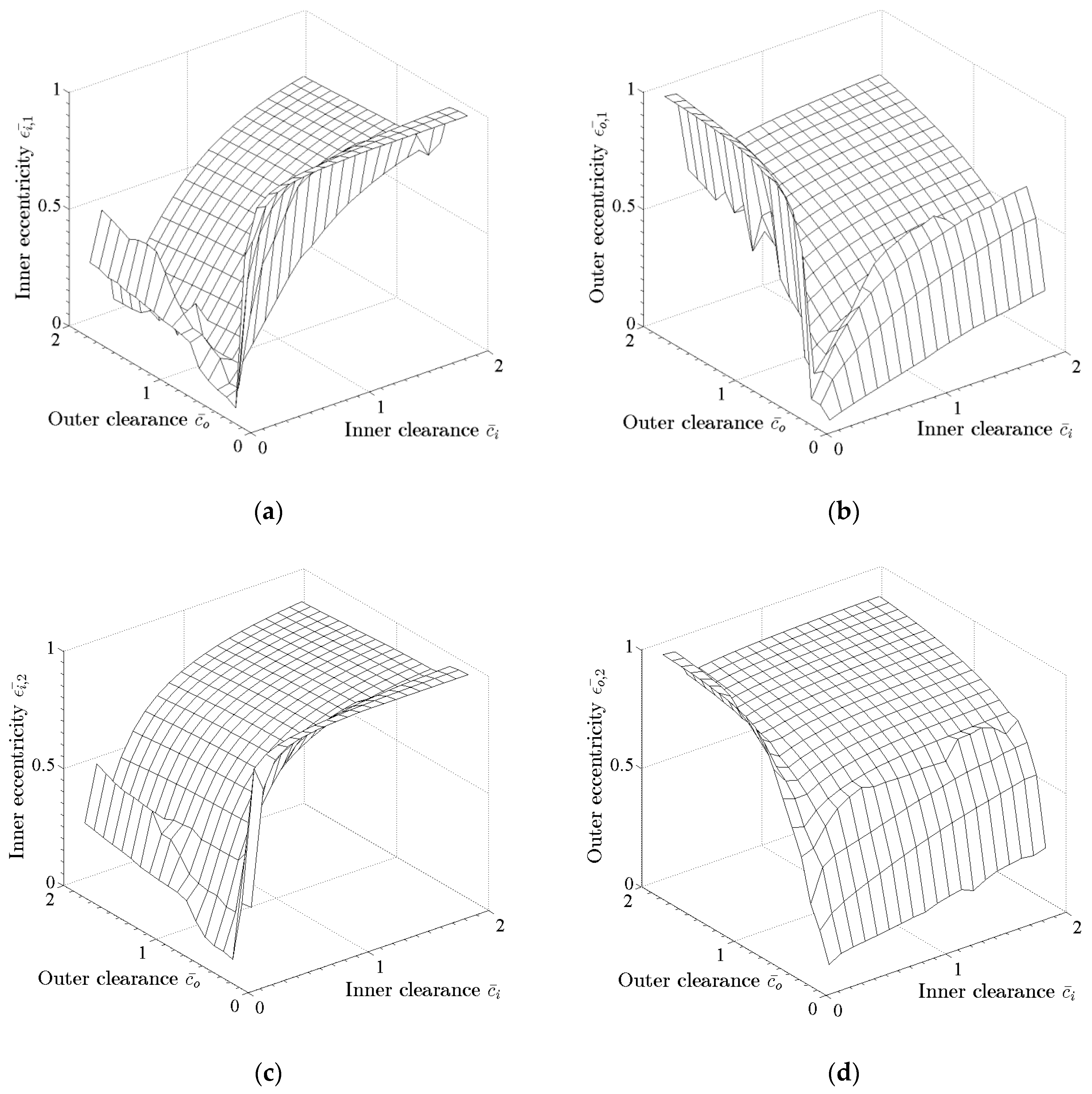
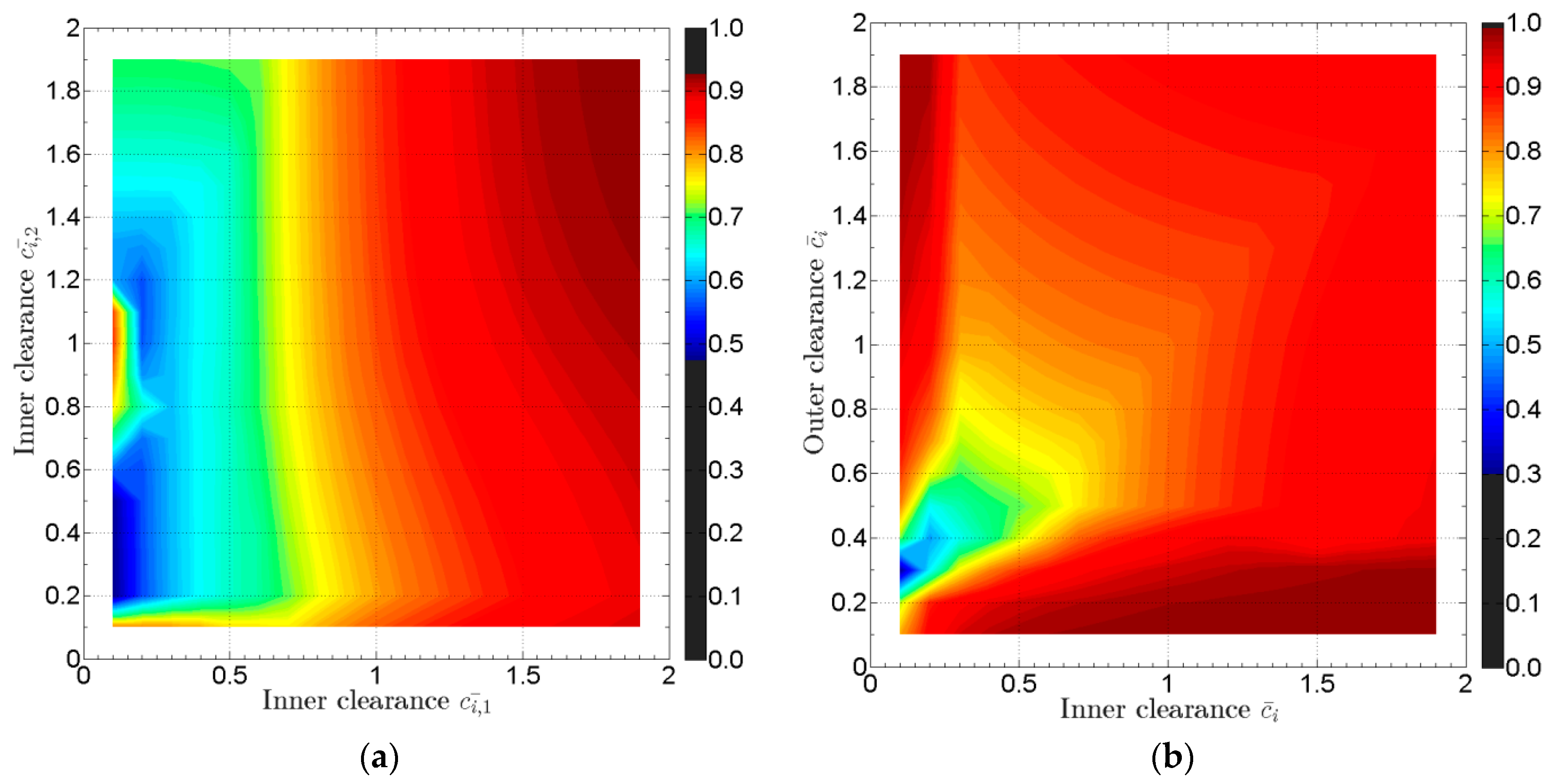
2.2. Application of the Method in Floating Ring Bearings

The application of the database method in floating rings is similar to what described in Section 2.1. The reader should consider that although the floating ring bearings in this paper consider a plain circular profile, the formulation is generic and it can be applied to any floating ring bearing profile, elliptical or other, including holes and grooves. This is to motivate simulation of lobe bore floating rings in future. Should the inner and outer films be of different length to diameter ratio 1 / k , a different database should be calculated. This is the most applicable case in floating rings of automotive turbochargers [16,17].
In correspondence to Section 2.1, the lubrication problem in a floating ring bearing which is the evaluation of lubricant pressure distribution in the inner and the outer film for laminar, isothermal, and isoviscous flow is defined by the Reynolds equation which is now written in correspondence to Equation (5), in Equation (17) for the inner, and in Equation (18) for the outer film respectively, including the geometric and the physical parameters defined in Figure 2. Note that the coordinate system is now defined in Figure 2, and that in the inner film the rotating speed included in Reynolds is Ω + Ω r . In Equations (17) and (18), c i and c o is the inner and outer clearance respectively. The bearing has a length L B , i and L B , o in the inner and the outer film respectively in X direction, the lubricant is characterized by a dynamic viscosity μ i in the inner film and μ o in the outer film, both assumed constant in this paper. The shaft rotates around its center with a rotating speed Ω and the ring obtains a rotating speed Ω r as the inner and outer film apply torques T i and T o respectively, see also Figure 2b. Under dynamic conditions, the shaft and the ring will perform whirling motion inside the bearing clearances, with absolute velocities z ˙ s , y ˙ s , and z ˙ r , y ˙ r . Equations (20)–(23) complete the definition of the Reynolds equation in Equations (17) and (18).
θ ( H i 3 p i ¯ θ ) + k i 2 H i 3 2 p i ¯ x ¯ i 2 = ( 6 ε z , i 12 ε ¯ ˙ y , i ) sin θ ( 6 ε y , i + 12 ε ¯ ˙ z , i )   cos θ
θ ( H o 3 p ¯ o θ ) + k o 2 H o 3 2 p ¯ o x ¯ o 2 = ( 6 ε z , o 12 ε ¯ ˙ y , o ) sin θ ( 6 ε y , o + 12 ε ¯ ˙ z , o )   cos θ
{ H i H o } = { h i / c i h o / c o } ,           { h i h o } = { c i ( z s z r ) · cos ( θ ) ( y s y r ) · sin ( θ ) ,   inner   film c o z r · cos ( θ ) y r · sin ( θ ) ,                                                     outer   film
p ¯ i = c i 2 p i μ i ( Ω + Ω r ) R 2 ,   ε z , i = z s z r c i ,   ε y , i = y s y r c i ,   ε ˙ z , i = z ˙ s z ˙ r c i , ε ˙ y , i = y ˙ s y ˙ r c i
ε ¯ ˙ z , i = ε ˙ z , i Ω + Ω r , ε ¯ ˙ y , i = ε ˙ y , i Ω + Ω r ,   k i = 2 R L B , i ,   x ¯ i = 2 x L B , i ,   φ i ˙ = ( z s z r ) ( y ˙ s y ˙ r ) ( y s y r ) ( z ˙ s z ˙ r ) ε z , i 2 + ε y , i 2  
p ¯ o = c o 2 p o μ o Ω r R o 2 ,   ε z , o = z r c o ,   ε y , o = y r c o ,   ε ˙ z , o = z ˙ r c o , ε ˙ y , o = y ˙ r c o
ε ¯ ˙ z , o = ε ˙ z , o Ω r , ε ¯ ˙ y , o = ε ˙ y , o Ω r ,   k o = 2 R o L B , o ,   x ¯ o = 2 x L B , o ,   φ o ˙ = z r y ˙ r y r z ˙ r ε z , o 2 + ε y , o 2    
Similarly to Section 2.1, the Reynolds equation in the form of Equations (17) and (18) is divided by Q i and Q o respectively, where ε i = e i / c i , φ ¯ ˙ i = φ ¯ ˙ i / ( Ω + Ω r ) = φ ˙ i / ( c i 2 ( Ω + Ω r ) ) and ε o = e o / c o , φ ¯ ˙ o = φ ¯ ˙ o / Ω r = φ ˙ o / ( c o 2 Ω r ) . Then, the Reynolds equation can be written in Equations (24) and (25). The variables x ¯ 1 , i x ¯ 2 , i x ¯ 1 , o x ¯ 2 , o are defined in Equations (26)–(28).
3 H i 2 H θ , i p ¯ i θ + H i 3 2 p ¯ i θ 2 + k i 2 H i 3 2 p ¯ i x ¯ i 2 = 6 x ¯ 1 , i sin θ 6 x ¯ 2 , i cos θ
3 H o 2 H θ , o p ¯ o θ + H o 3 2 p ¯ o θ 2 + k o 2 H o 3 2 p ¯ o x ¯ o 2 = 6 x ¯ 1 , o sin θ 6 x ¯ 2 , o cos θ    
Similarly, to the portion Q defined in Equations (7) and (8), the portions Q i and Q o have two definitions, each, as follows.
For the inner film:
  • If | ε z , i 2 ε ¯ ˙ y , i | > | ε y , i + 2 ε ¯ ˙ z , i | , then Q i   =   |   ( ε z , i 2 ε ¯ ˙ y , i ) ( ε i 2 ( Ω + Ω r ) 2 ε z , i ε ¯ ˙ y , i + 2 ε y , i ε ¯ ˙ z , i ) ε i ( ε z , i ( Ω + Ω r ) 2 ε ¯ ˙ y , i ) |
  • If | ε z , i 2 ε ¯ ˙ y , i | < | ε y , i + 2 ε ¯ ˙ z , i | , then Q i   =   |   ( ε y , i + 2 ε ¯ ˙ z , i ) ( ε i 2 ( Ω + Ω r ) 2 ε z , i ε ¯ ˙ y , i + 2 ε y , i ε ¯ ˙ z , i ) ε i ( ε y , i ( Ω + Ω r ) + 2 ε ¯ ˙ z , i ) |
For the outer film:
  • If | ε z , o 2 ε ¯ ˙ y , o | > | ε y , o + 2 ε ¯ ˙ z , o | , then Q o   =   |   ( ε z , o 2 ε ¯ ˙ y , o ) ( ε o 2 Ω r 2 ε z , o ε ¯ ˙ y , o + 2 ε y , o ε ¯ ˙ z , o ) ε o ( ε z , o Ω r 2 ε ¯ ˙ y , o ) |
  • If | ε z , o 2 ε ¯ ˙ y , o | < | ε y , o + 2 ε ¯ ˙ z , o | , then Q o   =   |   ( ε y , o + 2 ε ¯ ˙ z , o ) ( ε o 2 Ω r 2 ε z , o ε ¯ ˙ y , o + 2 ε y , o ε ¯ ˙ z , o ) ε o ( ε y , o Ω r + 2 ε ¯ ˙ z , o ) |
The Reynolds equation in the form of Equations (24) and (25) has variables defined in Equations (26) and (27).
p ¯ i = p ¯ i Q ,       p ¯ i θ = p ¯ i θ ,       x ¯ 1 , i = ε z , i 2 ε ¯ ˙ y , i Q i ,     x ¯ 2 , i = ε y , i + 2 ε ¯ ˙ z , i Q i
p ¯ o = p ¯ o Q ,   p ¯ o θ = p ¯ o θ ,   x ¯ 1 , o = ε z , o 2 ε ¯ ˙ y , o Q o , x ¯ 2 , o = ε y , o + 2 ε ¯ ˙ z , o Q o
The derivatives of the inner and outer fluid film thickness functions appearing in Equations (24) and (25) are defined in Equation (28).
H θ , i = H i θ = ε x , i sin θ ε y , i cos θ       ,         H θ , o = H o θ = ε x , o sin θ ε y , o cos θ  
Equations (24) and (25) are solved with the four variables x ¯ 1 , x ¯ 2 , ε x , ε y (inner or outer) to receive specific values in the domain (−1,1). The solution is a numerical solution scheme e.g., Finite Difference Method. Supposing that the FDM is implemented, with a definition of finite difference grid as N z × N θ , the respective intervals are defined as Δ z = L B / N z , for inner or outer film, and Δ θ = 2 π / N θ . Similarly, to Section 2.1 two cases are defined for the evaluation of p ¯ for inner or outer film, these being for Q > 0 , and Q < 0 . The inner and outer film impedance forces and friction torques are then evaluated in correspondence to Equations (9)–(11).

3. Evaluation of Nonlinear Transient Response Using the Bearing Database Method

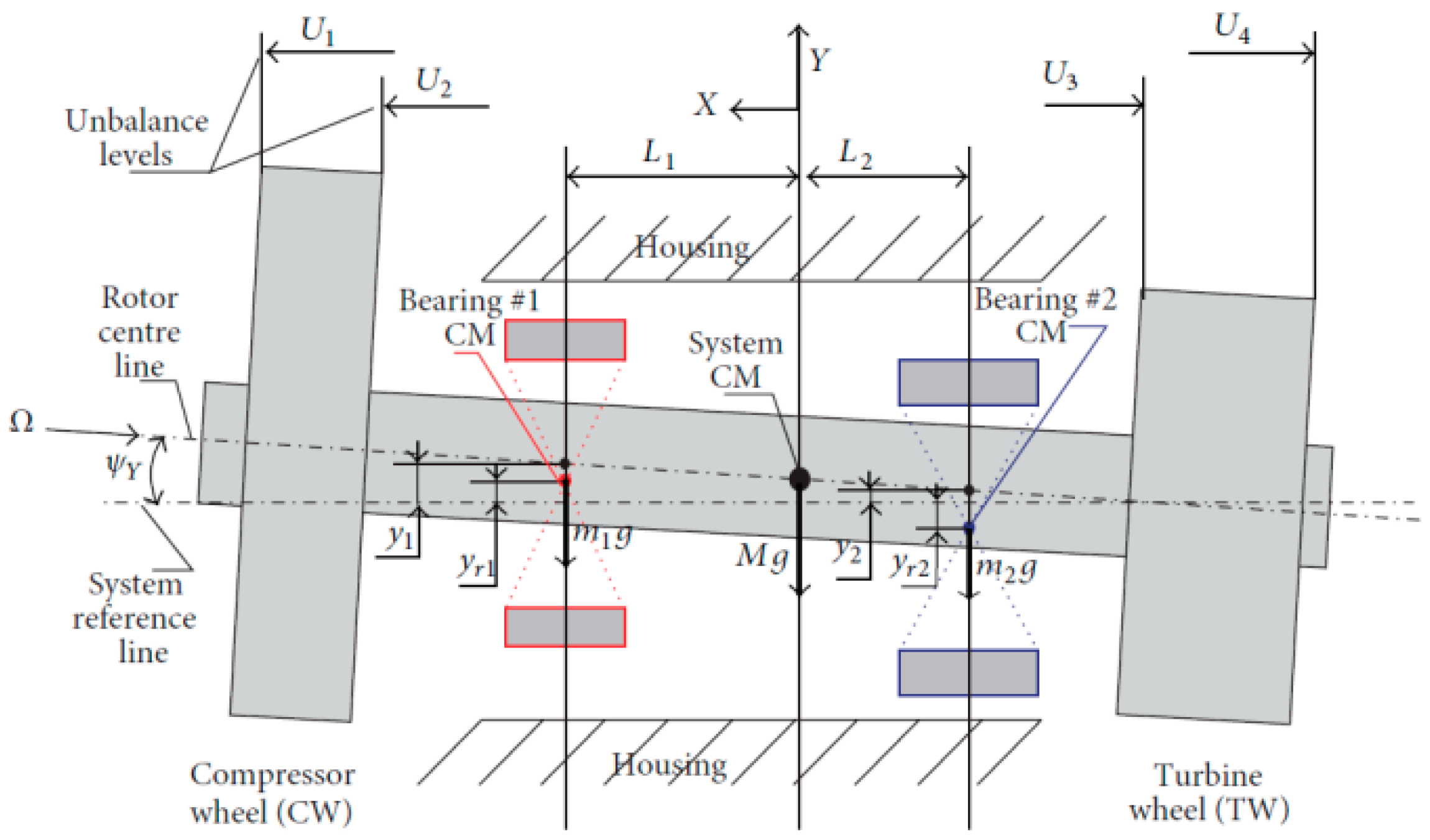
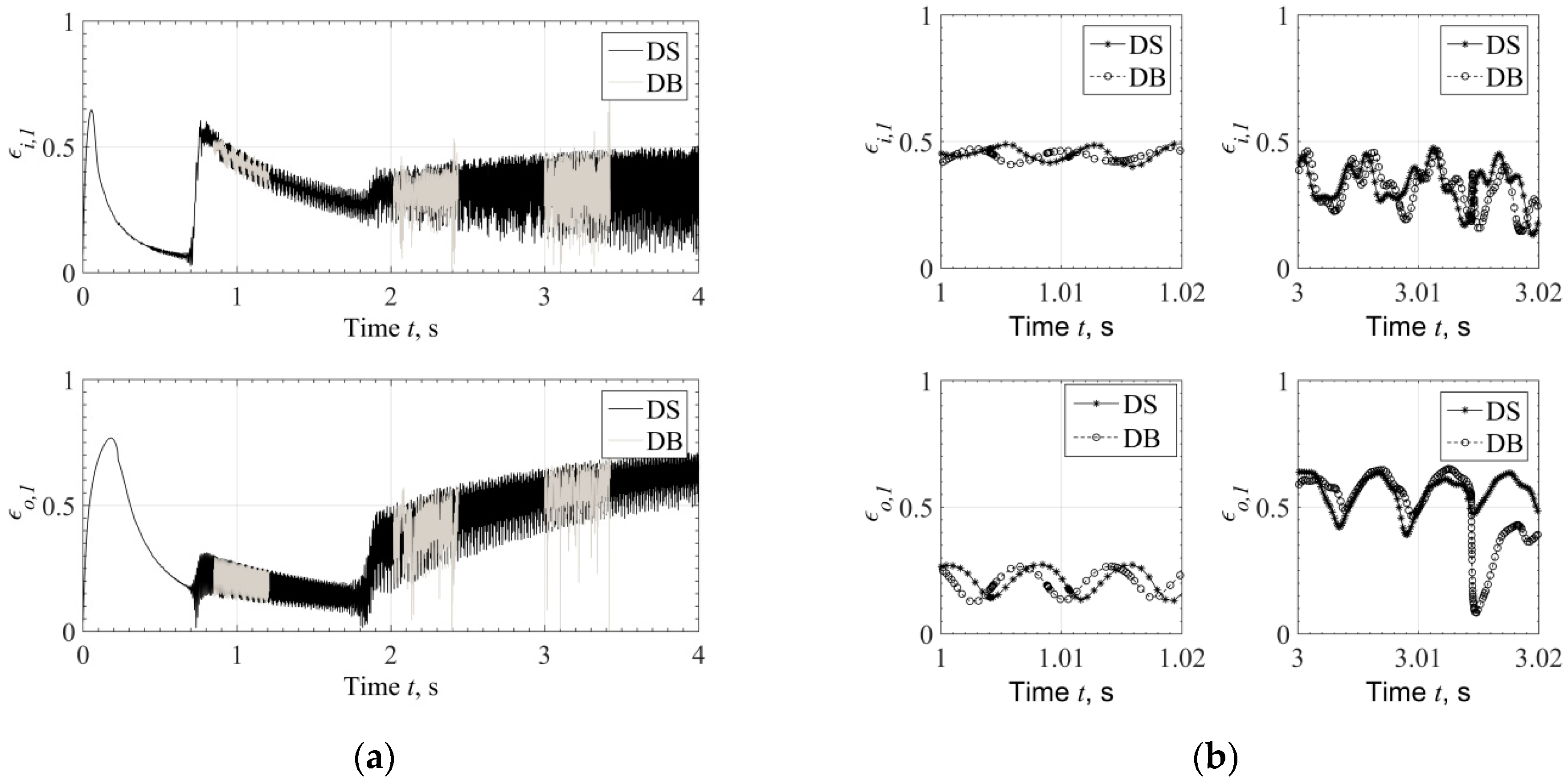
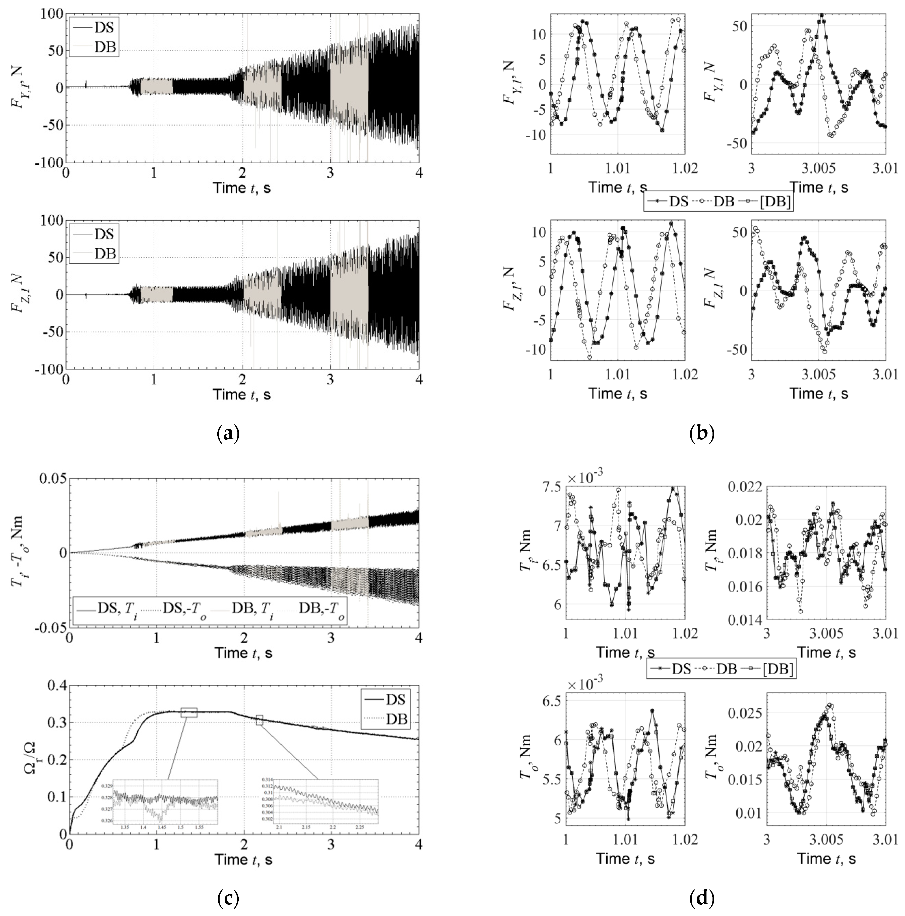
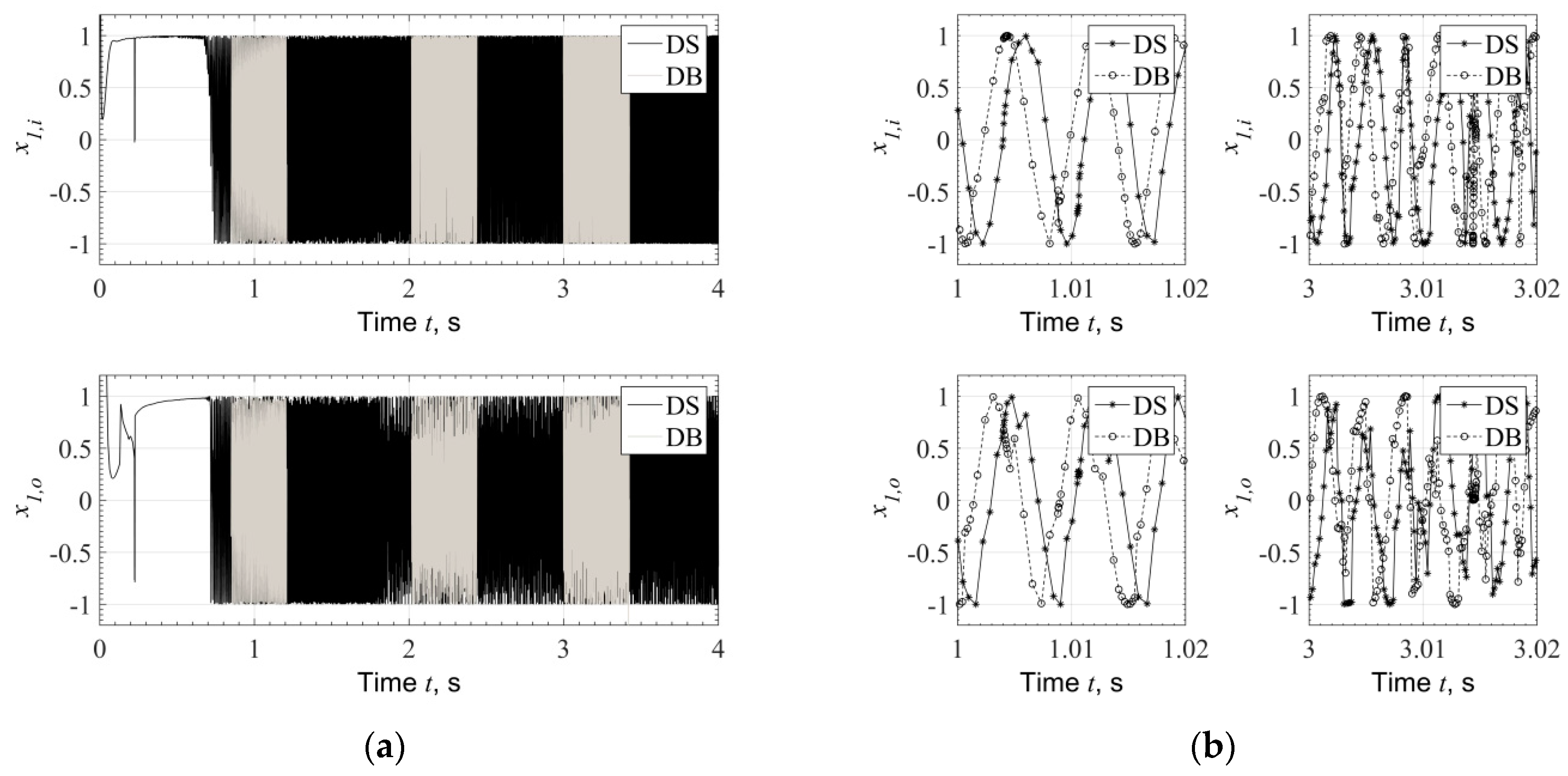
3.1. Application in a High-Speed System of Automotive Turbocharger

A simplified rotor system of an automotive turbocharger is used in this Section to obtain transient response through two different bearing algorithms [17]:
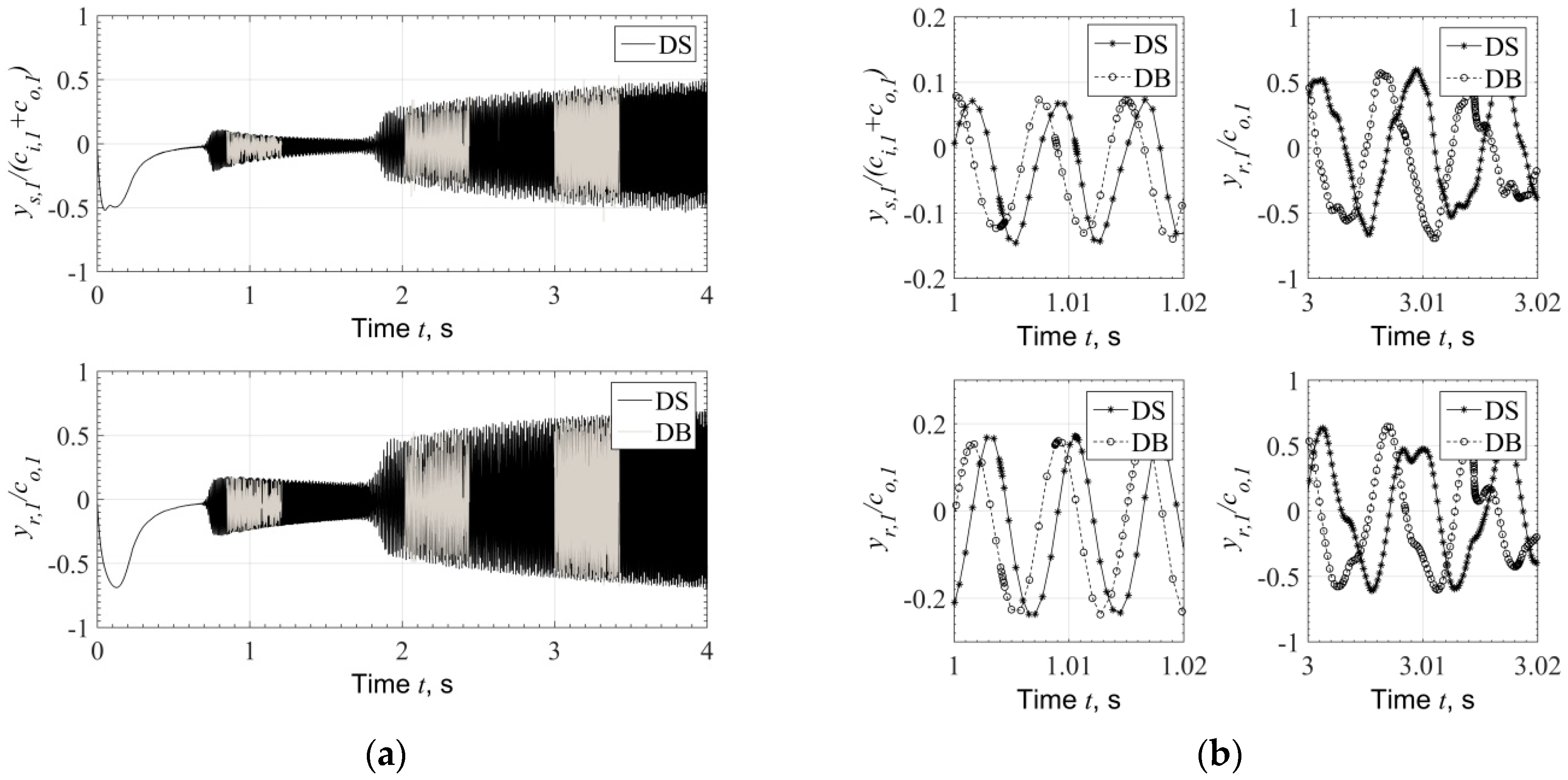
  • Bearing forces are called from the Ordinary Differential Equation solver (ODE solver) and provided by the database which has been constructed as described in previous sections;
  • Bearing forces are called from the ODE solver and they are evaluated with the direct solution of the Reynolds equation at every discrete time during run-up, using Finite Difference Method.
The second case will be referred in the results as ‘‘Direct Solution’’, while the first as “Database Method”. The reader may advise recent works on enhanced bearing models and rotordynamics of automotive turbochargers, including phenomena and methods which are beyond the scope of this paper [21,22,23,24,25,26,27,28,29,30,31].
A rigid rotor and two wheels representing the turbine wheel and the compressor wheel, see Figure 3, as lumped masses at rotor ends, consist a rotor which rotates with a speed Ω around the rotor center line, as shown in Figure 3. The total mass of CW, TW, and Rotor is M , the total moment of inertia (polar) is J P with respect to the rotor center line, and the total diametric moment of inertia is J T with respect to the vertical and horizontal axes that pass through the center of mass of the system, see Figure 3. The mathematical modeling of the simplified high speed system of Figure 3 is presented in Appendix A.
A representative response of an automotive turbocharger with the equations of motion of Equation (A17) is depicted in Figure 4 and Figure 5, where the response and the inner and outer eccentricity of the journal and of the ring are plotted. One can notice the expected phenomenon of response ‘jumps’ each time that a hydrodynamic instability takes place, in the inner or outer film, at the Bearing 1 or Bearing 2. The floating ring bearing is supposed to suppress the response due to instability in inner film, with enhanced damping from the outer film. The reader may find extended studies on instability phenomena of such systems in [24,25,26,27].
The response plotted in Figure 4 has been evaluated with both methods (a) and (b) defined at the beginning of the Section, for the virtual time of 4 s, with linearly increasing rotating speed, Ω = 1800 · t   [ rad / s ] . The ending speed of the turbocharger is approximately Ω = 70   kRPM . This is an application of relatively large turbocharger for commercial Diesel application. Comparing the two methods, a very good agreement is noticed in the response amplitude during run-up, see Figure 4a.
The response evaluated by the Database Method (DB) is plotted only in selected time slots in Figure 4a so as not to cover the response evaluated by the Direct Solution (DS) and other response characteristics at selected time slots. However, when the response is plotted in very short time range, e.g., from 1 s to 1.02 s and from 3 s to 3.02 s, see Figure 4b, it is clear that the response evaluated through the two methods is not identical. The reason is that Database Method does not render identical to the Direct Method bearing forces and frictional torque at every discrete time step. However, taken into account also Figure 5, where the eccentricity is plotted, one can conclude that Bearing Database Method will not compromise the reliability of the results compared to the Direct Method. This is clear from Figure 4a and Figure 5a, where the rotor response and bearing eccentricity appear in very good agreement between the two methods.
For the response evaluated and plotted in Figure 4, useful time measures for the application of the Database Method are presented in Table 1. Both methods require similar calls in the bearing subroutines, these being approximately 2.45 Mio for the Direct Solution, and 2.37 Mio for the Database Method. This difference is due to the slightly different number calls to the system of differential equations, these being approximately 0.61 Mio in the Direct Solution, and 0.59 Mio in the Bearing Database. The occasional slight differences in the forces between the two methods are the reason for the minor differences on the dynamics and on the progress of the numerical solution. The total time spent in the calculation of bearing forces is drastically lower with the Database Method, this being 1.48 min, compared to the Direct Solution which requires 207 min in bearing subroutines. This is a ratio of approximately 140 times faster Database Method. The Database Method returns the bearing forces and frictional force in 0.037 ms, while the Direct Solution requires 5.06 ms. This is the same ratio as mentioned before, 140 times faster Database Method. However, the total time for the run-up and the evaluation of the response is not that faster when Database Method is used; Direct Solution evaluates the response in 213 min, while Database Method requires only 8 min, which is approximately 27 times faster. This is a difference which highlights the benefit from the application of Database Method. All computations in this paper were performed with a desktop PC with an i7 CPU @ 2.30GHz.
In Figure 6, the fluid film forces and the frictional torque are compared between the two methods. With a database of INT = 100 intervals, the Database Method bearing forces and frictional torque are in a very good agreement to the Direct Solution forces and torque during the rotor run-up, see Figure 6a,c (upper graph). Furthermore, the ring speed ratio is in very good agreement between the two methods, see Figure 6c (lower graph). A key notice is that when database Forces and torque are evaluated with input from the Direct Solution response, these are identical to the direct solution, see Figure 6b,d comparing the curves (DS) and ([DB]). The Database Method forces and torques evaluated with input from the Database Method response appear to some divergence from the Direct Solution forces and torque, comparing the curves (DS) and (DB) in Figure 6b,d. As mentioned above, the Database Method Response is not identical to the Direct Solution response, see Figure 4b and Figure 5b. This explains the last comment for the divergence of (DS) and (DB) curves in Figure 6b,d. However, the divergence in the forces and torque (comparing (DS) and (DB)) does not render a considerable difference in the response. The difference noticed in forces and torque comparing the two methods is due to the combined effect of the interpolation and of the different input (slightly different response) to the bearing algorithms. The computation time with the database method is approximately 136 times lower than this with the Direct Method, see Table 1 for time related measures. Two points of interest is that a relatively small rotor may develop bearing impedance forces of approximately 100 N amplitude, see Figure 6a, and that the frictional torque in inner and outer film of the floating ring bearings develops a variance, approximately after 1.8 s, see Figure 6c, due to the pressure variance from the rotor and ring whirling motion. The variance is the torque does not render intense variance in ring speed as shown in Figure 6c where only a slight variance in the ring speed may be depicted (not clear in the full curve of Figure 6c, see the two zoom windows inside Figure 6c).
The Right Hand Side Reynolds input parameters x ¯ 1 and x ¯ 2 included in Equation (6) present similar progress to each other with their values to be limited in the domain −1 < x ¯ 1 , x ¯ 2 < 1, as described in previous Section. In Figure 7, the variation of x ¯ 1 is presented for the inner and outer film separately in Figure 7a during the entire rotor run-up. As the system experiences its first instability at approximately 0.8 s, the variation of x ¯ 1 occurs in the entire range from −1 to 1, at both films of Bearing 1. Similar progress is noticed in the films of Bearing 2. The values x ¯ 1 , x ¯ 2 are depended only to the kinematics of the journal and of the ring, therefore, as the Database Method response is slightly different to the Direct Solution response, see also Figure 4b, the respective values of x ¯ 1 , x ¯ 2 appear with some divergence, see Figure 7b. The boundaries of x ¯ 1 , x ¯ 2 is the basement of the method presented in this paper as they render a bounded the Reynolds equation regardless the kinematics of the journal and the ring, see Section 2.
The drastically reduced computation time for impedance forces and frictional torque of bearing designs of multiple inputs, allows design optimization schemes [31] as the one presented in continue. As the response of the turbocharger cannot be evaluated with closed form expressions to render analytical functions of inputs, these being the physical and geometrical properties of the bearing and outputs like response, temperature, and others needed for the bearing design, the rotordynamic engineer has to perform several case studies where the response is calculated numerically for various combinations of input parameters. This set of calculations may include from few up to hundredths virtual run-ups of the system, and for each of them, the designated output is plotted. Such a case is shown in Figure 8, where the inner and outer eccentricity at both bearings (output) of the turbocharger of Figure 3, is plotted as a function of inner and outer bearing clearances (input). The value of each eccentricity considered in the graphs of Figure 8 is the higher eccentricity noticed in the entire run-up time (0–4 s). The clearance values are expressed with respect to a reference design clearance, and the range of variation is from 0.1 to 1.9, with an interval of 0.15. Therefore 144 run-up simulations have to be performed for this optimization problem. With the time related measures presented in Table 1, the optimization problem requires more than 21 days computational time using the Direct Method, while the Database Method requires less than 1 day computational time.
The optimization problem may consider the maximum eccentricity calculated at every fluid film simultaneously, meaning that for each of the 144 run-up simulations, the m a x ( ε 1 , i ,   ε 1 , o ,   ε 2 , i ,   ε 2 , o ) can be plotted. Constructing contour plots for the progress of m a x ( ε 1 , i ,   ε 1 , o ,   ε 2 , i ,   ε 2 , o ) can be produced in as shown in Figure 9. In Figure 9a the optimization problem considers variation of inner clearance in both bearings, while Figure 9a considers the variation of both inner and outer clearances as in Figure 8. Selecting a limit for the output parameter as e.g., m a x ( ε 1 , i ,   ε 1 , o ,   ε 2 , i ,   ε 2 , o ) < 0.6 , the optimization problem can render the group of design inputs that satisfy the rotordynamic standards.
Furthermore, the fact that the Database Method offers drastically reduced evaluation time, enables the rotordynamic optimization problem with e.g., 4 or 5 parameters varying simultaneously, like inner clearance, outer clearance, bearing distance, bearing length. This consideration is practically applied with an objective function and the computational time is always restriction on how many parameters varying and at how many intervals. In Figure 9 there are acceptable combinations of clearances such that m a x ( ε 1 , i ,   ε 1 , o ,   ε 2 , i ,   ε 2 , o ) < 0.6 . These combinations are gathered in low values of clearances (tight clearances) as depicted in Figure 9b. However, the rotordynamic engineer should consider that other parameters, like e.g., oil temperature are influenced from tight clearances, and therefore a limit must be applied in the lower “acceptable” combinations.

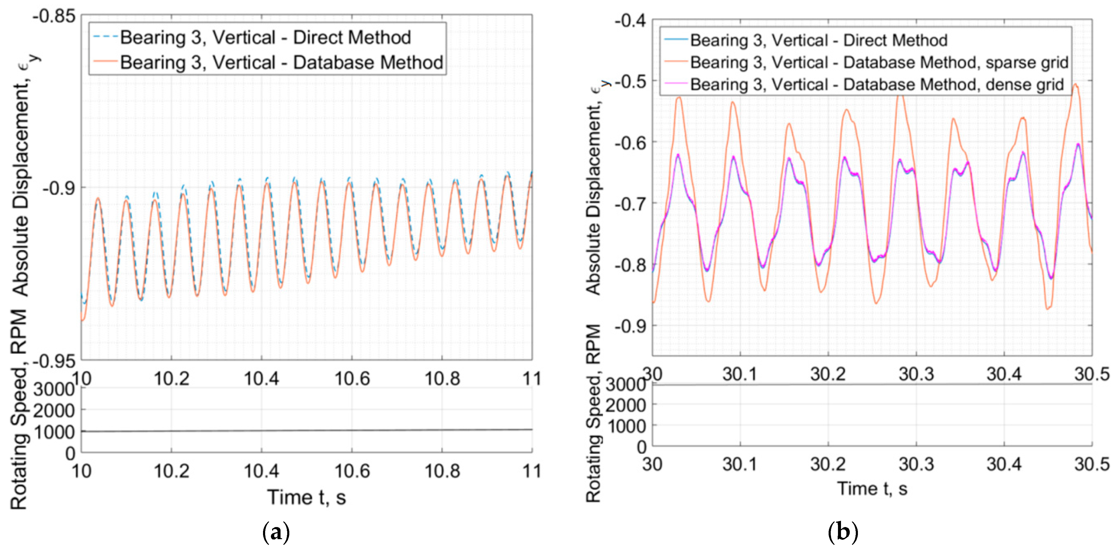
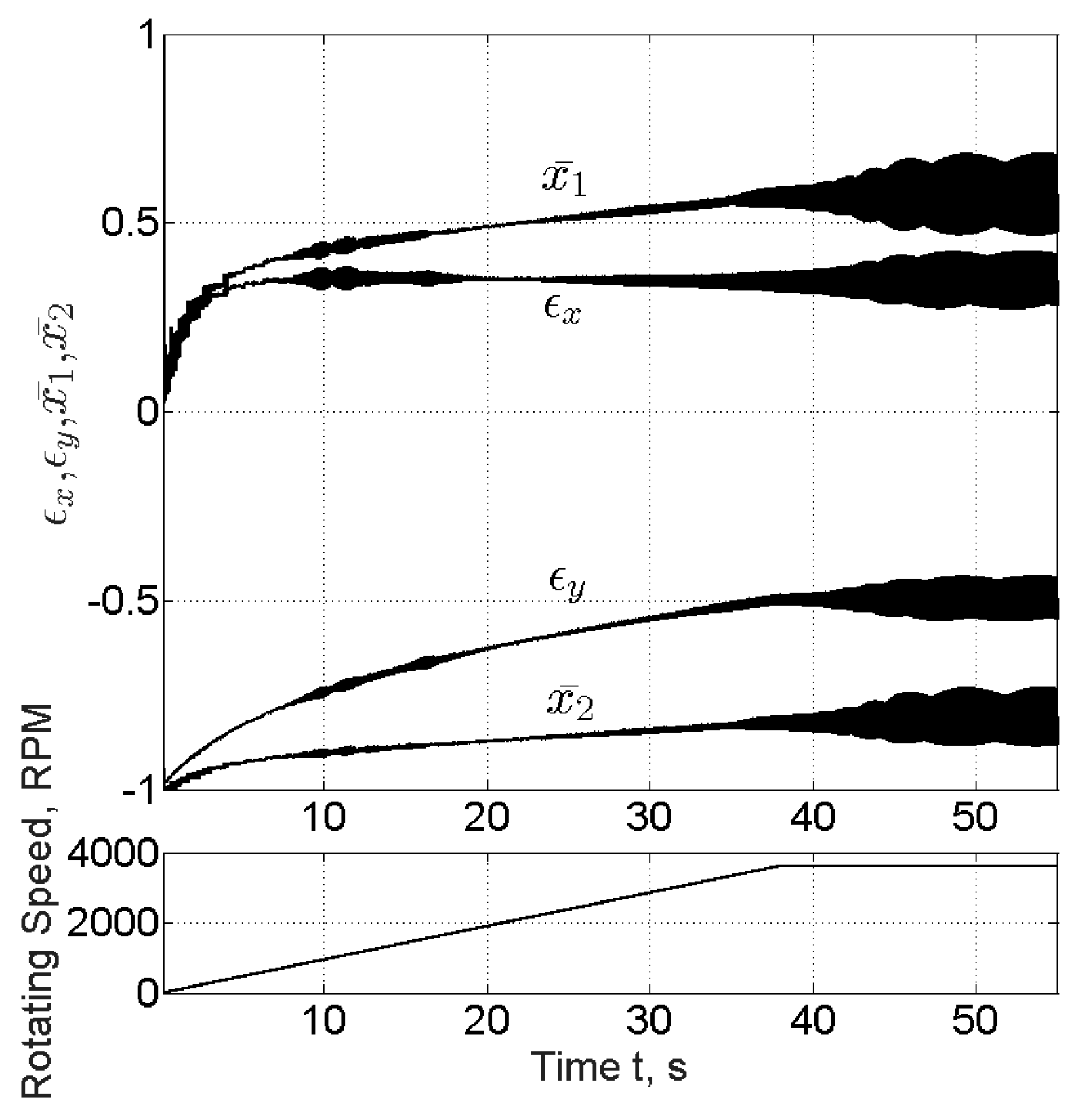
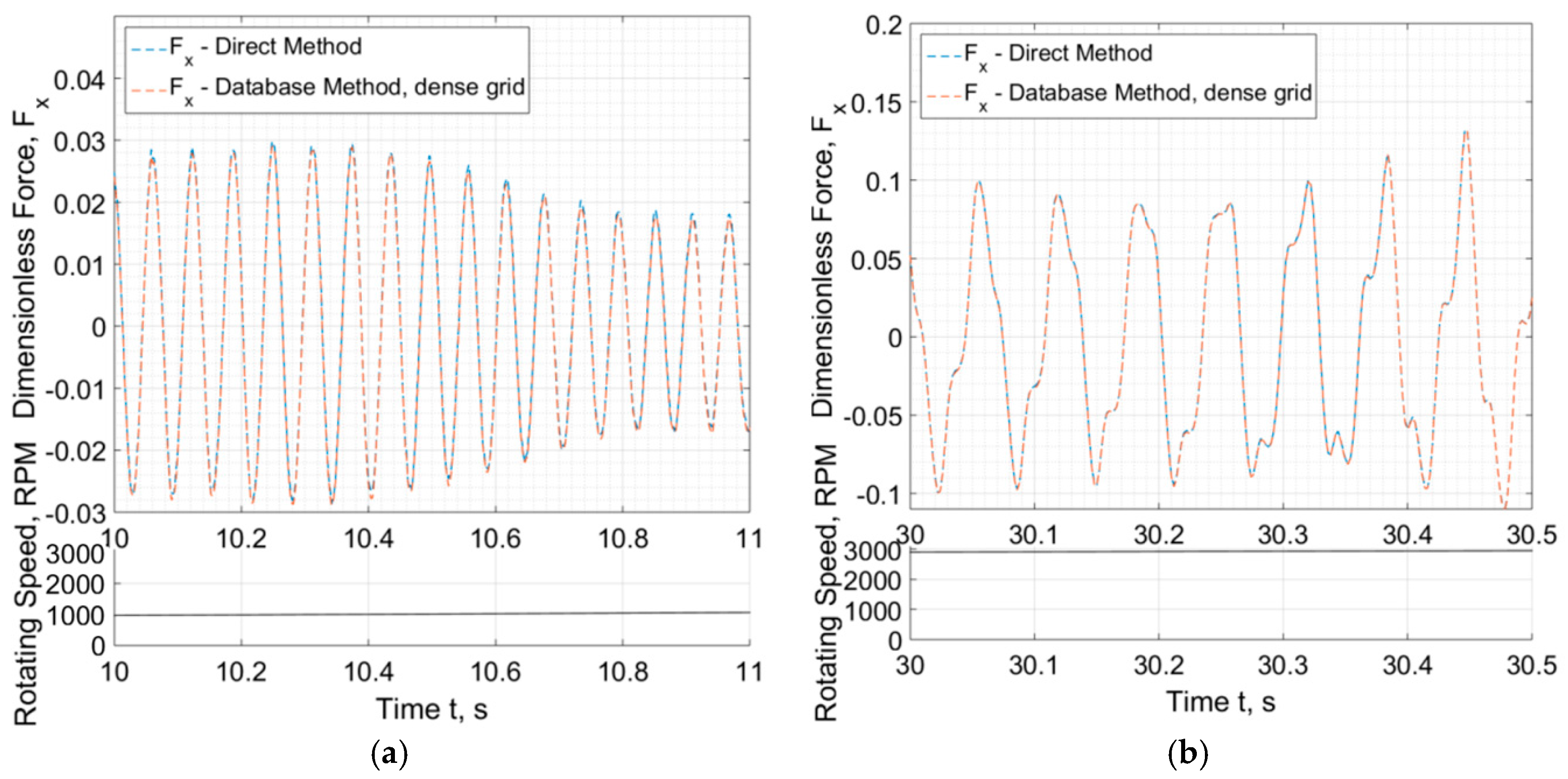
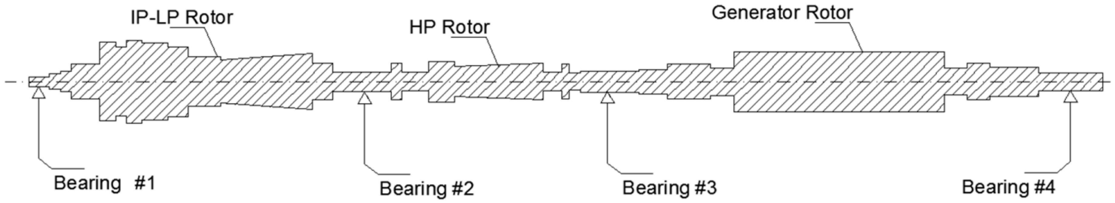
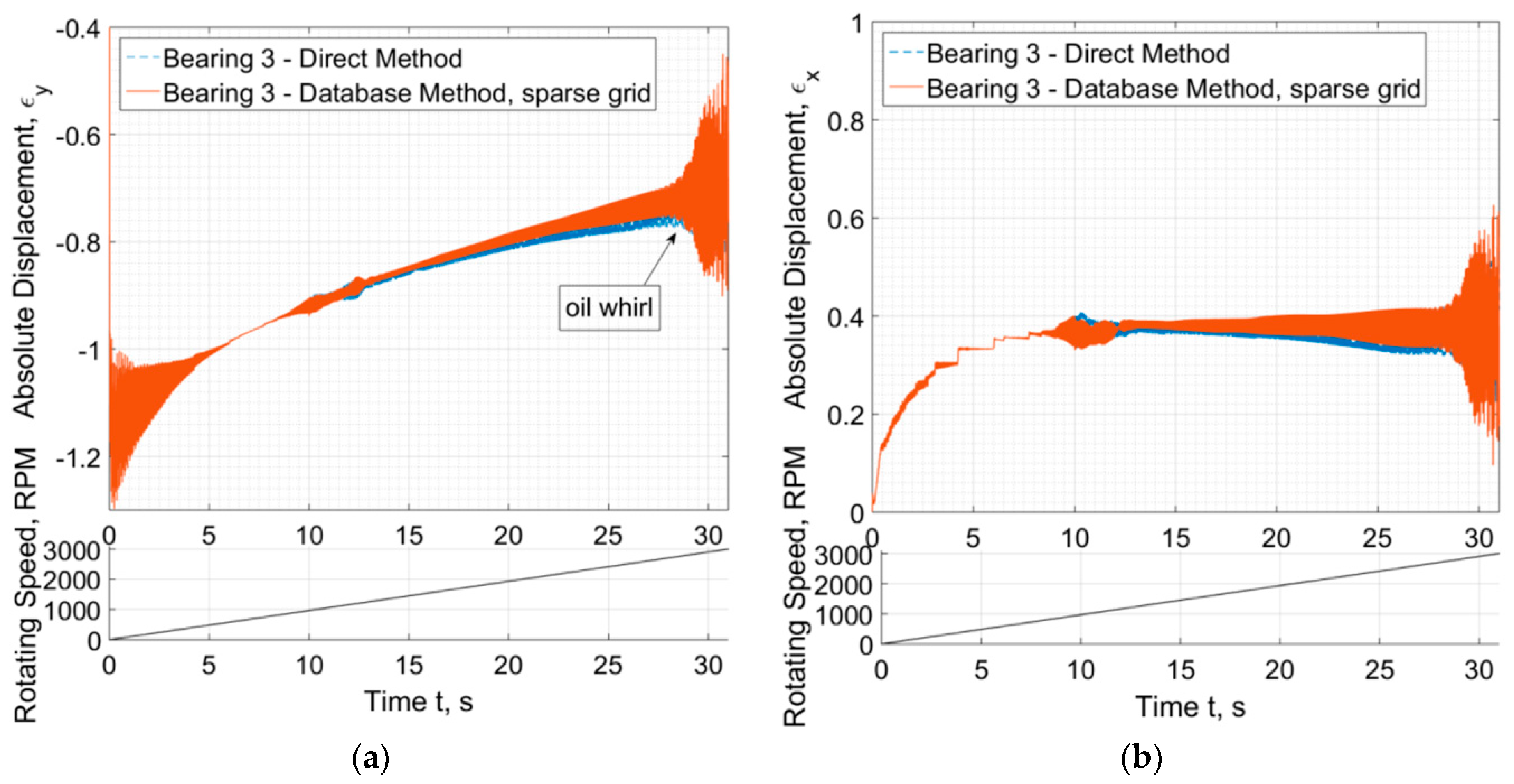
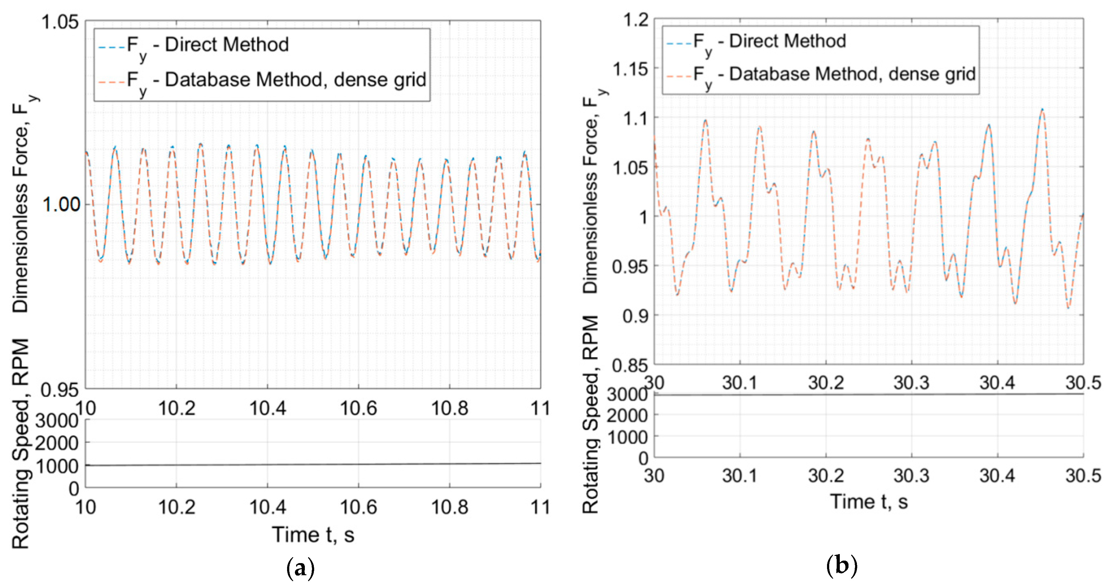
3.2. Application in a Medium-Speed System of Turbine-Generator Shaft-Train

The database method in its extended form, as described in Section 2.1, is applied in a rotor bearing system of turbine generator for power generation, represented in Figure 10 [18]. The system consists of three rotors and four journal bearings mounted on the respective pedestals as depicted in Figure 1b.
The profile of the journal bearings consists of a combination of partial arcs. The central partial arc is concentric to the bearing center (no preload), while the two partial arcs on the sides of the central are preloaded, see Figure 1a. The bearings have different L/D ratios, while the ratio of pad clearance to journal radius is equal in all bearings. Therefore, due to the fact that length to diameter ratio is different, all bearings require a separate database. The lubricant dynamic viscosity is considered equal in all bearings. Thermal effects are not taken into account in the evaluation of bearing performance. However, thermal effects can be considered in the database method as already mentioned in Section 2.
A virtual run-up of the rotor system is performed from 0 to 3000 RPM with a linearly varying rotating speed for the time duration of 30 s. Unbalance excitation is considered in all three rotors in positions so that 1st, 2nd, and 3rd mode of each rotor can be excited, and the unbalance magnitude is defined per ISO. The rotor system response develops some transient phenomena at the beginning of the run-up, as the initial condition locates the system approximately at the center of each bearing. Approximately after 5 s these transients are quenched and the rotor journals continue with elevation towards the center of the bearing as the rotating speed increases, see Figure 11a. The first critical speed of the generator rotor appears at c.a. 11 s (1100 RPM) with a horizontal mode, and approximately at 13 s (1300 RPM) with a vertical mode. Only the response at Bearing #3 is considered in Figure 11. In Figure 11b, where the horizontal response is plotted, a stepped progress appears approximately between 3 s and 7 s; this is due to the low relative accuracy of the numerical solver at this stage of response so as the solver to proceed fast to the transient response during passage through resonance which is of more interest for the dynamics of the system. The solver implements dynamic time interval and varying relative accuracy.
As the rotor approaches the speed of 2800 RPM, instability occurs and the system enters a supercritical Hopf bifurcation, where under constant rotating speed the system whirls at a stable limit cycle of constant shape (extent). However, the rotating speed is increased further (end speed is 3000 RPM) so as to achieve a higher response and to study the efficiency of the database method in such a case; this is why an unstable design has been chosen in this Section. Figure 11 depicts that a sparse database of 100 intervals (INT = 100) is efficient to evaluate an accurate (compared to Direct Method) response only at relatively low amplitudes. It is clear that after the 15 s, a slight divergence appears between the responses evaluated with the two methods for bearing forces.
The difference is clearer in Figure 12 where the response is plotted at a narrow time slot. In Figure 12a, the sparse grid (INT = 100) is efficient to render accurate response (close to the response evaluated through the direct method) when the response is low (e.g., at 10 s—1000 RPM). When the response amplitude increases (e.g., during instability at 30 s), the sparse grid is not sufficient as severe divergence appears between the two methods. A dense grid of e.g., INT = 600 intervals is then required to render an excellent much between the two methods (also INT = 400 can be sufficient but of not that excellent match). The number of INT = 600 intervals is high enough, and the database requires severely higher time to be computed. It is redundant to say that the database is calculated in advance of the rotordynamic calculations.
The progress of the four input parameters in the database ( ε x , ε y , x ¯ 1 , and x ¯ 2 ) is depicted in Figure 13 for the corresponding run-up shown in Figure 11. These four parameters will be always varying in −1 < ε x , ε y , x ¯ 1 , x ¯ 2 < 1, and therefore, according to Figure 13, somebody can realize that an interval of e.g., 1/INT = 0.01 (sparse grid) might be large compared to 1/INT = 0.002 (dense grid). Figure 14 and Figure 15 show the efficiency of the database method to predict identical to the direct method forces in all circumstances of small journal whirling around an equilibrium position (e.g., at 10 s, see Figure 14a and Figure 15a) or large journal whirling on a limit cycle (e.g., at 30 s during instability, see Figure 14b and Figure 15b).
Table 2 depicts computational time used for the response of the system with the two methods. Bearing forces are returned from the database method subroutine in only 0.037 ms (the same as calculated for a single oil film in the floating ring bearing in previous section) while the direct method subroutine will return forces in 5.06 ms. This is a reduction of approximately 136 times. The time on the database subroutine (from call to return) will be retained at the same low level (e.g., 0.037 ms at the specific CPU) whatever the method for the lubrication performance is. Depending on the rotor-bearing system (type of application), low or high number of degrees of freedom is used for the rotor model, and as a result, it may happen that the reduction of the net time spent in the bearing routines is not enough to decrease the total time of a rotor run-up. For instance, a turbocharger transient run-up with a rotor model as a rigid body will experience a severe reduction on evaluation time when the database method is used, as the number of DOFs is low (even 10 DoFs are enough to model such system as shown in previous section), and therefore the run-up time is influenced much from the bearing subroutines. At the current example the total time for rotor run-up is reduced almost 3 times when using the database method, see Table 2. All computations in this paper were performed with a desktop PC with an i7 CPU @ 2.30GHz.

4. Conclusions

Standard rotordynamic design evaluation of large turbomachinery does not include nowadays evaluation of nonlinear transient response due to the still high evaluation time which cannot support design procedures. However, in small turbochargers and turbopumps, and generally in high speed turbomachinery, nonlinear transient analysis is mandatory for the prediction of dynamics and therefore of mechanical integrity and operating performance in order to establish an initial design. The evaluation time spent in bearing subroutines is still considerable, and this paper aims to support the introduction of bearing database modules to the rotordynamic calculations of large and small turbomachinery. Enhanced THD bearing models are to be included in database method in future works. The method can implement enhanced THD bearing models without the evaluation time to be a drawback. However, this application is not included in this paper.
Large turbomachinery does not urge nonlinear transient response for the calculation of unbalance response (linear harmonic analysis yields very similar results in most cases), but, the nonlinear stability analysis may be proved very beneficial as slender rotors (which cannot be avoided—e.g., generator rotors) operate very close to the stability threshold (e.g., 60 Hz generators).
The present paper aims to provide the tool for a faster evaluation of transient nonlinear response. With the reduction of the evaluation time, the rotordynamic engineer may compose optimization problems including more input design parameters than before. Regarding the evaluation time of nonlinear transient response of high speed systems (mandatory for their design), this can be severely reduced and optimization problems including the definition of clearances, groove dimensions, bearing length, etc. can be performed, without the time to be a drawback, even with enhanced THD models. Conclusively, the following benefits of using the database method should be highlighted:
  • The method renders severe time reduction in transient nonlinear response calculation of large and small scale systems of high and medium speed and enables nonlinear rotordynamics in standard design procedures (fast design iteration);
  • The method enables the implementation of accurate bearing models (e.g., THD, CFD) of complex bearing geometries in rotordynamic algorithms without any time cost (regardless the complexity of bearing performance model);
  • The rotordynamic predictions comparing Database Method and Direct Solution are in a very good agreement, if not identical.
Time related measures from the computations performed in this paper prove the drastically reduced computation time for a high speed rotor run-up from 0 to 70 kRPM to approximately 8 min, while direct solution required 213 min (26 times less). This is a system with 10 DoFs and the response computation time is intensively influenced from the bearing model. For the turbine shaft train, in which several DoFs were modelled, 80 h were required with the direct solution and 28 h with the database to compute a run-up of the system from 0 to 3000 RPM. The evaluation time spent solely on the call-return of one bearing subroutine is reduced from 5.06 ms to 0.0037 ms; the bearing database returns the oil film forces and frictional torque approximately 136 times faster than the direct method (solution of the Reynolds and calculation of forces).

Author Contributions

Conceptualization, A.C.; methodology, A.C.; software, A.C.; validation, J.-C.L.; formal analysis, A.C.; investigation, A.C.; resources, A.C.; data curation, J.-C.L.; writing—original draft preparation, A.C.; writing—review and editing, J.-C.L.; visualization, A.C.; supervision, A.C.; project administration, A.C.; funding acquisition, A.C.

Funding

This research received no external funding.

Conflicts of Interest

The authors declare no conflict of interest.

Nomenclature

Hellenic Letters
ε :relative eccentricity θ Ε :starting angle of the fluid film
ε i :inner relative eccentricity θ S :ending angle of the fluid film
ε o :outer relative eccentricity ϑ 1 :rotating angle of the ring 1
ε x :horizontal relative eccentricity ϑ 2 :rotating angle of the ring 2
ε y :vertical relative eccentricity ϑ ˙ 1 :rotating speed of the ring 1
ε x , i :horizontal inner relative eccentricity ϑ ˙ 2 :rotating speed of the ring 2
ε y , i :vertical inner relative eccentricity ϑ ¨ 1 :rotational acceleration of the ring 1
ε x , o :horizontal outer relative eccentricity ϑ ¨ 2 :rotational acceleration of the ring 2
ε y , o :vertical outer relative eccentricity φ ˙ :journal attitude angle rate of change
ε ˙ x :rate of change of ε x φ ¯ ˙ :dimensionless rate of change of φ
ε ˙ y :rate of change of ε y φ ¯ ˙ i :dimensionless rate of change of φ i
ε ˙ y , i :rate of change of ε y , i φ ¯ ˙ o :dimensionless rate of change of φ o
ε ˙ y , o :rate of change of ε y , o φ ¯ ˙ :dimensionless φ ˙
ε ¯ x ˙ : ε ˙ x / Ω φ ¯ ˙ i :dimensionless rate of change of φ i
ε ¯ y ˙ : ε ˙ y / Ω φ ¯ ˙ o :dimensionless rate of change of φ o
ε ¯ ˙ y , i : ε ˙ y , i / ( Ω + Ω r ) ψ Y :vertical tilting angle of the rigid rotor
ε ¯ ˙ y , o : ε ˙ y , o / Ω r ψ Z :horiz. tilting angle of the rigid rotor
ε ¯ ˙ z , i : ε ˙ z , i / ( Ω + Ω r ) Ω:rotating speed of the shaft
ε ¯ ˙ z , o : ε ˙ z , o / Ω r Ω ˙ :rotating accel. of the shaft
μ:dynamic viscosity of lubricant Ω r :rotating speed of the ring
μ i :dynamic viscosity of the inner film Ω r , 1 :rotating speed of the ring 1
μ o :dynamic viscosity of the outer film Ω r , 2 :rotating speed of the ring 2
θ :circumferential coordinate angle Ω ˙ r , 1 :rotating accel. of the ring 1
Ω ˙ r , 2 :rotating accel. of the ring 2
Latin Letters
c B :bearing clearance F Y , i :inner fluid film force, vertical
c i :inner bearing clearance F Y , o :outer fluid film force, vertical
c o :outer bearing clearance F Y , 1 :inner fluid film force, Bearing 1, vert.
c P :pad clearance F Y , 2 :inner fluid film force, Bearing 2, vert.
C P , X :damping coef. in pedestal (horiz.) F Z , i :inner fluid film force, horizontal
C P , Y :damping coef. in pedestal (vert.) F Z , o :outer fluid film force, horizontal
D:diameter of shaft F Z , 1 :inner fluid film force, Bearing 1, horiz.
e :absolute eccentricity (of journal) F Z , 2 :inner fluid film force, Bearing 2, horiz.
e i :inner absolute eccentricity (of journal) F i G :gravitational force at node
e o :outer absolute eccentricity (of ring) F u , y , j :unbalance forces, vertical
F i :field matrix F u , z , j :unbalance forces, horizontal
F g , 1 :gravity forces loading bearing 1 F X B :nonlinear bearing force, horizontal
F g , 2 :gravity forces loading bearing 2 F X U :unbalance forces, horizontal
F Y U :unbalance forces, vertical M P , X :lumped pedestal mass, horiz.
F Y B :nonlinear bearing force, vertical M P , Y :lumped pedestal mass, vert.
F ¯ x :dimensionless bearing force, horiz. N z :pressure intervals (axially)
F ¯ x + :dimensionless bearing force, horiz. N θ :pressure intervals (circumf.)
F ¯ x :dimensionless bearing force, horiz. p :absolute pressure
F ¯ y :dimensionless bearing force, vert. P i :point matrix
F ¯ y + :dimensionless bearing force, vert. p ¯ :dimensionless pressure
F ¯ y :dimensionless bearing force, vert. p ¯ i :inner dimensionless pressure
g :gravity acceleration p ¯ o :outer dimensionless pressure
h:fluid film thickness p ¯ : p ¯ / Q
h i :inner fluid film thickness Q :divisor of dimen/less Reynolds
h o :outer fluid film thickness R B :journal radius
H :dimensionless fluid film thickness R L : bearing lobe radius
R :radius of shaft
H i :dimensionless fluid film thick., inner t :time
H o :dimensionless fluid film thick., out. T i :torque of the inner film
I P , 1 :mass moment of inertia of ring 1 T i :transfer matrix
I P , 2 :mass moment of inertia of ring 2 U :unbalance magnitude
J P :rotor mass moment of inertia, polar T o : torque of the outer film
J T :rotor mass moment of inertia, diametric U j :distance of unbalance plane distance
J N D , i :lumped mass moment of inertia, diam. x j :horizontal displacement
J N P , i :lumped mass moment of inertia, polar x P :pedestal displacement, horiz.
k :bearing ratio, 2 R B / L B x ˙ j :journal absolute velocity, horiz.
K P , X :Stiffness coefficient of pedestal, horiz. y j :journal displacement, horiz.
K P , Y :Stiffness coefficient of pedestal, vert. y P :pedestal displacement, vert.
L:bearing length in axial direction y r :ring displacement, vert.
L B :bearing length in axial direction y s :journal displacement, vert.
L B , i :bearing length in the inner film, axially direction y ˙ j :journal absolute velocity, vert.
L B , o :bearing length in the outer film, axially direction y ˙ r :ring absolute velocity, vert.
L 1 :length of bearing 1 y ˙ s :journal absolute velocity, vert.
L 2 :length of bearing 2 z :axial coordinate in bearing
m :bearing preload (geometric) z r :ring displacement, horiz.
m 1 :mass of ring 1 z s :journal displacement, horiz.
m 2 :mass of ring 2 z ˙ r :ring absolute velocity, horiz
M :total mass of rotor z ˙ s :journal absolute velocity, horiz
M N , i :lumped mass at a node z ¯ :Dimensionless axial coordinate

Appendix A. Simplified Model of an Automotive Turbocharger

For the representative high speed system of a rigid rotor mounted on floating ring bearings, see Figure 3, four ODEs describe the motion of the rotor system, these defined in Equations (A1)–(A4) with the resulting impedance forces from the bearings to the rotor to be F Y , 1 and F Y , 2 in the vertical direction and F Z , 1 and F Z , 2 in the horizontal direction, for Bearing #1 and Bearing #2 correspondingly, see Figure 3.
M y ¨ C M = F g , 1 + F Y , 1 + F g , 2 + F Y , 2 + j = 1 4 F u , y , j
M z ¨ C M = F Z , 1 + F Z , 2 j = 1 4 F u , z , j
J T ψ ¨ Y + J P Ω ψ ˙ Ζ   = F Y , 1 L 1 F Y , 2 L 2 + F u , y , 1 U 1 + F u , y , 2 U 2 F u , y , 3 U 3 F u , y , 4 U 4
J T ψ ¨ Ζ J P Ω ψ ˙ Y = F Z , 1 L 1 F Z , 2 L 2 F u , z , 1 U 1 F u , z , 2 U 2 + F u , z , 3 U 3 + F u , z , 4 U 4
The unique nonlinearity in the 4 DoF system is sourced from the fluid film bearing forces. The four unbalance forces applied on the planes at a distance U j from the plane of CM (see Figure 3), are defined on Equation (A5) for constant rotating acceleration Ω ˙ .
F u , y , j = u j Ω 2 cos ( 1 2 Ω ˙ t 2 ) , F u , z , j = u j Ω 2 sin ( 1 2 Ω ˙ t 2 ) ,   j = 1 , 2 , 3 , 4
The gravity forces loading the two bearings are defined in Equation (A6).
F g , 1 = M g L 2 / ( L 1 + L 2 ) ,   F g , 2 = M g L 1 / ( L 1 + L 2 )
Using Equations (A7) and (A8), and after some math, the equations of motion in Equations (A1)–(A4) are written in Equations (A9) to (A12).
y 1 = y C M + L 1 ψ Y , y 2 = y C M L 2 ψ Y , z 1 = z C M + L 1 ψ Z , z 2 = z C M L 2 ψ Z
ψ Y = y 1 y 2 L 1 + L 2    ψ Z = z 1 z 2 L 1 + L 2
y ¨ 1 = L 1 + L 2 M L 2 ( F g , 1 + F Y , 1 + F g , 2 + F Y , 2 + j = 1 4 F u , y , j ) L 1 L 2 y ¨ 2
z ¨ 1 = L 1 + L 2 M L 2 ( F Z , 1 + F Z , 2 j = 1 4 F u , z , j ) L 1 L 2 z ¨ 2
y ¨ 2 = L 1 + L 2 J T ( F Y , 1 L 1 F Y , 2 L 2 + F u , y , 1 U 1 + F u , y , 2 U 2 F u , y , 3 U 3 F u , y , 4 U 4 ) + J P Ω J T ( y ˙ 1 y ˙ 2 ) + z ¨ 1
z ¨ 2 = L 1 + L 2 J T ( F Z , 1 L 1 F Z , 2 L 2 F u , z , 1 U 1 F u , z , 2 U 2 + F u , z , 3 U 3 + F u , z , 4 U 4 ) J P Ω J T ( z ˙ 1 z ˙ 2 ) + y ¨ 1
The floating rings in this paper are assumed for simplicity as plain hollow cylindrical rigid bodies. Torsional moments act at each floating ring from the inner and the outer film of the lubricant, see Figure 2b. The fluid film forces applied on the ring from the outer film are defined as F Y , o and F Z , o in the vertical and horizontal direction correspondingly, see Figure 2b, while the inner film forces are defined as F Y , i and F Z , i in the vertical and horizontal direction correspondingly, see Figure 2b. The respective torsional moments are defined as T i and T o for inner and outer film correspondingly, see Figure 2b. The gravity forces are also incorporated assumed to act on the vertical direction at the CM of each ring with magnitudes m 1 g and m 2 g .
Each floating ring rotates by ϑ 1 and ϑ 2 , with rotating speed Ω r , 1 = ϑ ˙ 1 and Ω r , 2 = ϑ ˙ 2 and rotational acceleration Ω ˙ r , 1 = ϑ ¨ 1 and Ω ˙ r , 2 = ϑ ¨ 2 respectively. With the definitions in Figure 2 and Figure 3, the equations of motion for each floating ring are given in Equations (A13)–(A15), and therefore, 6 more DoFs are added into the rotor-bearing system. In equations of motion for the floating rings, I P , 1 and I P , 2 is the mass moment of inertia of each ring with respect to its axis of rotation and m 1 and m 2 is the mass of each ring.
m 1 y ¨ r , 1 = m 1 g + F Y , o , 1 F Y , i , 1 , m 1 z ¨ r , 1 = F Z , o , 1 F Z , i , 1
m 2 y ¨ r , 2 = m 2 g + F Y , o , 2 F Y , i , 2 , m 2 z ¨ r , 2 = F Z , o , 2 F Z , i , 2
I P , 1 ϑ ¨ 1 = T i , 1 T o , 1 ,   I P , 2 ϑ ¨ 2 = T i , 2 T o , 2
After the definitions in Equation (A16), the 2nd order 10 × 10 system of motion equations, Equations (A7) to (A12), is reduced to a 1st order 20 × 20 system of motion equations in Equation (A17).
s ( 1 ) = y s , 1   ,   s ( 2 ) = y ˙ s , 1 ,   s ( 3 ) = y s , 2 ,   s ( 4 ) = y ˙ s , 2 ,   s ( 5 ) = z s , 1 s ( 6 ) = z ˙ s , 1 ,   s ( 7 ) = z s , 2 ,   s ( 8 ) = z ˙ s , 2 ,   s ( 9 ) = y r , 1 ,   s ( 10 ) = y ˙ r , 1 s ( 11 ) = z r , 1 , s ( 12 ) = z ˙ r , 1 ,   s ( 13 ) = ϑ 1 ,   s ( 14 ) = ϑ ˙ 1 ,   s ( 15 ) = y r , 2 s ( 16 ) = y ˙ r , 2 ,   s ( 17 ) = z r , 2 ,   s ( 18 ) = z ˙ r , 2 s ( 19 ) = ϑ 2 ,   s ( 20 ) = ϑ ˙ 2
The system s ˙ = f ( s ) can be solved applying numerical integration solvers for stiff ODE systems.
s ˙ ( 1 ) = s ( 2 ) s ˙ ( 2 ) = L 1 + L 2 L 2 M ( F g , 1 + F Y , 1 + F g , 2 + F Y , 2 + j = 1 4 F u , y , j ) L 1 L 2 s ˙ ( 4 ) s ˙ ( 3 ) = s ( 4 ) s ˙ ( 4 ) = L 1 + L 2 J T ( F Y , 1 L 1 F Y , 2 L 2 + F u , y , 1 U 1 + F u , y , 2 U 2 F u , y , 3 U 3 F u , y , 4 U 4 ) J P J T Ω ( s ( 6 ) s ( 8 ) ) s ˙ ( 5 ) = s ( 6 ) s ˙ ( 6 ) = L 1 + L 2 L 2 M ( F Z , 1 + F Z , 2 j = 1 4 F u , z , j ) L 1 L 2 s ˙ ( 8 ) s ˙ ( 7 ) = s ( 8 ) s ˙ ( 8 ) = L 1 + L 2 J T ( F Z , 1 L 1 F Z , 2 L 2 F u , z , 1 U 1 F u , z , 2 U 2 + F u , z , 3 U 3 + F u , z , 4 U 4 ) + J P J T Ω ( s ( 2 ) s ( 4 ) ) s ˙ ( 9 ) = s ( 10 ) s ˙ ( 10 ) = ( m 1 g F Y , i , 1 + F Y , o , 1 ) / m 1 s ˙ ( 11 ) = s ( 12 ) s ˙ ( 12 ) = ( F Z , i , 1 + F Z , o , 1 ) / m 1 s ˙ ( 13 ) = s ( 14 ) s ˙ ( 14 ) = ( T i , 1 T o , 1 ) / J P , 1 s ˙ ( 15 ) = s ( 16 ) s ˙ ( 16 ) = ( m 2 g F Y , i , 2 + F Y , o , 2 ) / m 2 s ˙ ( 17 ) = s ( 18 ) s ˙ ( 18 ) = ( F Z , i , 2 + F Z , o , 2 ) / m 2 s ˙ ( 19 ) = s ( 20 ) s ˙ ( 20 ) = ( T i , 2 T o , 2 ) / J P , 2

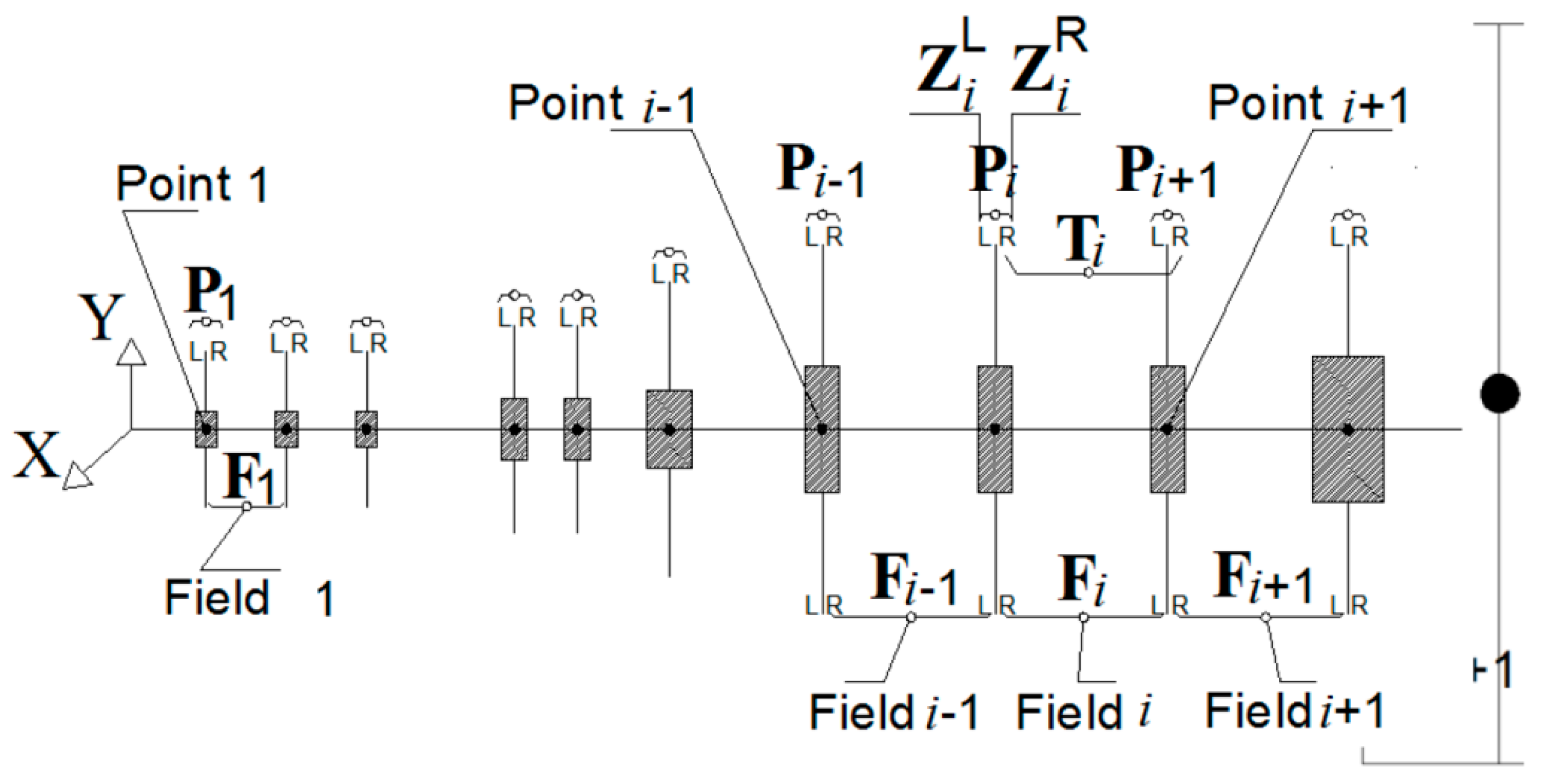
Appendix B. Modelling of Turbine-Generator Shaft Trains Using the Transient Transfer Matrix Method

The rotor-bearing-foundation system modeling used for the results of the turbine-generator system of Section 3.2 is presented in this Appendix B describing the Transient Transfer Matrix Method (TTMM) [19] which enables the evaluation of the nonlinear transient response of the system. Foundations are called also bearing pedestals or just pedestals in this Section. The Transfer Matrix Method is the core of the simulation of the system. The geometric and physical properties of multiple rotor segments N , are discretized in N + 1 nodes as lumped masses, see Figure A1.
The status vectors on the sides of each node Z i L and Z i R , i = 1 , 2 , , N + 1 , are defined as function of time t and the status vectors become as in Equation (A18), see also Figure A2. The displacements and the slopes on the sides of each lumped mass are equal, meaning that y i L ( t ) = y i R ( t ) = y i ( t ) , θ Y , i L ( t ) = θ Y , i R ( t ) = θ Y , i ( t ) and x i L ( t ) = x i R ( t ) = x i ( t ) , θ X , i L ( t ) = θ X , i R ( t ) = θ X , i ( t ) . The entire analysis considers the coordinate system defined in Figure A2.
Z i L ( t ) = { y i ( t ) θ Y , i ( t ) M Y , i L ( t ) V Y , i L ( t ) x i ( t ) θ X , i ( t ) M X , i L ( t ) V X , i L ( t ) 1 } T Z i R ( t ) = { y i ( t ) θ Y , i ( t ) M Y , i R ( t ) V Y , i R ( t ) x i ( t ) θ X , i ( t ) M X , i R ( t ) V X , i R ( t ) 1 } T
Figure A1. Conversion of a distributed mass system to a lumped mass system. Each segment’s mass is divided to nodes’ mass and the segments become massless.
Lubricants 07 00078 g0a1
Figure A2. The lumped mass system and the description of the fields and points that represent the segments and the nodes of the discretized system.
Lubricants 07 00078 g0a2
The role of the point matrix P i , field matrix F i , and transfer matrix T i , see also Figure A2 is expressed by the formulas Z i L ( t ) = F i × Z i 1 R ( t ) , Z i R ( t ) = P i × Z i L ( t ) , and T i = P i + 1 × F i . However, applying the Transient Transfer Matrix Method, there is no need to define the point matrix P i . The principle of the TTMM is based on that each nodal mass M N , i executes lateral and tilting transient motions under the effect of shearing and bending moment applied from the relative motions of the side nodal masses M N , i 1 and M N , i + 1 . Furthermore, the external forces acting to the mass M N , i , such as unbalance, gravitational forces, bearing impedance force etc., are incorporated. The equations of motion for the mass M N , i are given in Equation (A19).
M N , i x ¨ i = V X , i R V X , i L + F X B + F X U M N , i y ¨ i = V Y , i R V Y , i L + F Y B + F Y U F i G J N D , i θ ¨ X , i = M X , i R M X , i L J N P , i Ω θ ˙ Y , i J N D , i θ ¨ Y , i = M Y , i R M Y , i L + J N P , i Ω θ ˙ X , i
The unique source of nonlinearity in the system is the nonlinear bearing impedance forces F X B and F Y B . In order to evaluate the transient response of the system, the motion equations in Equation (A19) should be integrated with some numerical technique, e.g., Runge-Kutta. The MATLAB ODE solver® is highly recommended for such applications though. All forces and moments acting to the mass must be defined at each discrete time interval.
The status vectors Z i L and Z i R may be split in two vectors each, corresponding to the displacement/tilting and to the moments/forces as in Equation (A20).
Z D , i ( t ) = { y i ( t ) θ Y , i ( t ) x i ( t ) θ X , i ( t ) } T Z F , i R ( t ) = { M Y , i R ( t ) V X , i R ( t ) M X , i R ( t ) V Y , i R ( t ) } T Z F , i L ( t ) = { M Y , i L ( t ) V X , i L ( t ) M X , i L ( t ) V Y , i L ( t ) } T
Only one vector is needed at each node to describe the displacement/tilting of the mass, because these are equal. The moments/forces acting at the left and right of the mass M N , i are defined as Z F , i L ( t ) and Z F , i R ( t ) respectively. In this way, the expression Z i L ( t ) = F i × Z i 1 R ( t ) may be converted to the expression in Equation (A4) including the definitions of Equation (A20).
{ Z D , i ( t ) Z F , i L ( t ) } = [ F D D , i F D F , i F F D , i F F F , i ] × { Z D , i 1 ( t ) Z F , i 1 R ( t ) }
The submatrices F D D , i , F D F , i , F F D , i , and F F F , i are all ( 4 × 4 ) matrices defined in Equation (A22).
F D D , i = [ 1 L S , i 0 0 0 1 0 0 0 0 1 L S , i 0 0 0 1 ] , F F D , i = [ 0 ] ( 4 × 4 ) , F F F , i = [ 1 L S , i 0 0 0 1 0 0 0 0 1 L S , i 0 0 0 1 ] , F D F , i = [ L S , i 2 2 E i I S , i L S , i 3 6 E i I S , i + s f i L S , i G i A S , i 0 0 L S , i E i I S , i L S , i 2 2 E i I S , i 0 0 0 0 L S , i 2 2 E i I S , i L S , i 3 6 E i I S , i + s f i L S , i G i A S , i 0 0 L S , i E i I S , i L S , i 2 2 E i I S , i ]
Equation (B4) is expressed as a system of two equations with unknowns the force/moment vectors Z F , i L ( t ) and Z F , i 1 R ( t ) with its solution to be defined in Equations (A23) and (A24).
Z F , i 1 R ( t ) = F D F , i 1 × ( Z D , i ( t ) F D D , i × Z D , i 1 ( t ) )
Z F , i L ( t ) = F F D , i × Z D , i 1 ( t ) + F F F , i × ( F D F , i 1 × ( Z D , i ( t ) F D D , i × Z D , i 1 ( t ) ) )
Equations (A23) and (A24) simply express that if the displacement vectors are known in all nodes, then the force vectors can be evaluated in all nodes. The force vectors will be the input for the definition of motion equations of each mass in Equation (A19). Note that Equation (A23) and (A24) can be written for i = 2 , 3 , , N + 1 . Then, for an initial condition for every Z D , i , and for i = 1 , 2 , , N + 1 , the resulting bending moment and shearing force on the left and on the right side of each node i will be given from Equation (A25), excluding the values for the left of the 1st node Z F , 1 L and for the right of the last node Z F , N + 1 R . These should be set equal to zero since they correspond to free-end boundary conditions, meaning that Z F , 1 L = Z F , N + 1 R = { 0 0 0 0 } T . Should a different boundary condition be applied, the corresponding vectors are defined for Z F , 1 L and Z F , N + 1 R .
M X , i L ( t ) = Z F , i L [ 3 ] M Y , i L ( t ) = Z F , i L [ 1 ] , V   X , i L ( t ) = Z F , i L [ 2 ] V Y , i L ( t ) = Z F , i L [ 4 ] , M X , i R ( t ) = Z F , i R [ 3 ] M Y , i R ( t ) = Z F , i R [ 1 ] , V   X , i R ( t ) = Z F , i R [ 2 ] V Y , i R ( t ) = Z F , i R [ 4 ]
If any unbalance force is assigned to a node this should be defined in vertical and horizontal direction with the formulas of Equation (A26) for constant rotating speed Ω , and of Equation (A27) for linearly varying rotating speed (run-up/down) Ω = a t (where a = Ω ˙ ). Unbalance U is given first.
F Y U = U Ω 2 cos ( Ω t ) ,   F X U = U Ω 2 sin ( Ω t )
F Y U = U Ω 2 cos ( 0.5 Ω ˙ t 2 ) ,   F X U = U Ω 2 sin ( 0.5 Ω ˙ t 2 )
The initial values for the transient analysis should correspond to a position of the rotor that locates each journal inside the bearing clearance, preferably at the center of each bearing. This means that for example an approximate zero value for all displacements and tilting angles may be used if no pedestal elevation has been implemented, see Equation (A28).
Z D , i ( 0 ) = { y i ( 0 ) θ Y , i ( 0 ) x i ( 0 ) θ X , i ( 0 ) } T = 1 e 6 { 1 1 1 1 } T
At the case that an elevation of pedestals should be implemented due to static alignment, then the initial values for Z D , i ( 0 ) should correspond to the static sag line of the rotor to locate each journal in the center of the elevated bearing shell. The last input to define the system of motion equations for each mass is the gravitational force acting in every mass M N , i , given as F i G = M N , i g .
Motion equations compose a 4 × 4 system of 4 ODEs of 2nd order. To integrate the system and obtain the response over time, the system is converted to an 8 × 8 system composed by 8 ODEs of 1st order. The correspondence of the state variables q i to the displacement and tilting angle of each mass is given in Equation (A29). Then, the motion equations for the lumped masses of the rotor are defined in Equation (A30).
{ x i x ˙ i y i y ˙ i φ X , i φ ˙ X , i φ Y , i φ ˙ Y , i } T = { q i [ 1 ] q i [ 2 ] q i [ 3 ] q i [ 4 ] q i [ 5 ] q i [ 6 ] q i [ 7 ] q i [ 8 ] } t T
q ˙ i [ 1 ] = q i [ 2 ] q ˙ i [ 2 ] = 1 M N , i ( V X , i R V X , i L + F X B + F X U ) q ˙ i [ 3 ] = q i [ 4 ] q ˙ i [ 4 ] = 1 M N , i ( V Y , i R V Y , i L + F Y B + F Y U F i G ) q ˙ i [ 5 ] = q i [ 6 ] q ˙ i [ 6 ] = 1 J N D , i ( M X , i R M X , i L J N P , i Ω q i [ 8 ] ) q ˙ i [ 7 ] = q i [ 8 ] q ˙ i [ 8 ] = 1 J N D , i ( M Y , i R M Y , i L + J N P , i Ω q i [ 6 ] )
The system in Equation (A13) should be defined for every nodal mass, meaning for i = 1 , 2 , , N + 1 for a rotor with N segments. Bearing forces F X B and F Y B , and unbalance forces are introduced F X U and F Y U when in the respective node a bearing or unbalance is assigned. The pedestal motion is introduced in the transient analysis very similarly to the way that rotor’s masses motion was modeled. Considering Figure 1b, the pedestal mass translational motion may be described by a 2 × 2 system of 2 ODEs of 2nd order in Equation (A31).
M P , Y y ¨ P = K P , Y ( y P y P , 0 ) C P , Y y ˙ P F Y B M P , Y g M P , X x ¨ P = K P , X x P C P , X x ˙ P F X B
In Equation (A31) the excitation to the pedestal motion is introduced only by the resulting oil film forces F X B and F Y B of the bearing. With the definition of state variables in Equation (A32), pedestal motion equations are converted to a 4 × 4 system of 4 ODEs of 1st order in Equation (A33). The oil film bearing forces couple the two systems of Equations (A30) and (A32) with the nonlinear oil film force model to account for the motion of the pedestal (bearing shell).
{ y P , j y ˙ P , j x P , j x ˙ P , j } T = { w j [ 1 ] w j [ 2 ] w j [ 3 ] w j [ 4 ] } t T
w ˙ j [ 1 ] = w j [ 2 ] w ˙ j [ 2 ] = 1 M P , Y ( K P , Y ( w j [ 1 ] y P , 0 ) + C P , Y w j [ 2 ] + F Y B + M P , Y g ) , w ˙ j [ 3 ] = w j [ 4 ] w ˙ j [ 4 ] = 1   M P , X ( K P , Z w j [ 3 ] + C P , X w j [ 4 ] + F X B )
The initial value for the integral solution of system in Equation (A33) may be zero or non-zero depending on the elevation of the pedestal y P , 0 , see Equation (A34). The system should be defined for each pedestal, meaning that j = 1 , 2 , , NOB , where NOB is the number of bearings.
{ w i [ 1 ] w i [ 2 ] w i [ 3 ] w i [ 4 ] } 0 T = { 0 0 0 0 } T { w i [ 1 ] w i [ 2 ] w i [ 3 ] w i [ 4 ] } 0 T = { y P , 0 0 0 0 } T
As a summary to this Section, it should be clarified that a rotor with N segments, N + 1 nodal masses and NOB bearings will render n = ( N + 1 ) 8 + ( NOB ) 4 equations of motion with the equal number of unknowns, consisting a nonlinear autonomous system (when unbalance is absent) of the form x ˙ = f ( x , Ω ) .

References

  1. Sfyris, D.; Chasalevris, A. An exact analytical solution of the Reynolds equation for the finite journal bearing lubrication. Tribol. Int. 2012, 55, 46–58. [Google Scholar] [CrossRef]
  2. Chasalevris, A.; Sfyris, D. Evaluation of the finite journal bearing characteristics, using the exact analytical solution of the Reynolds equation. Tribol. Int. 2013, 57, 216–234. [Google Scholar] [CrossRef]
  3. Wang, W.; Zhang, Z. Nonlinear oil film force database. J. Shangai Univ. Technol. 1993, 14, 299–305. [Google Scholar]
  4. Wen, W.; Zhang, Z.; Chen, X. Application of the non-stationary oil film force database. J. Shanghai Univ. (Engl. Ed.) 2001, 5, 230–233. [Google Scholar]
  5. Chen, Z.; Jiao, H.; Xia, S.; Huang, W.; Zhang, Z. An efficient calculation method of nonlinear fluid film forces in journal bearings. Trib. Trans. 2002, 45, 324–329. [Google Scholar] [CrossRef]
  6. Wang, Y.; Liu, Z.; Kang, W.; Yan, J. Approximate analytical model for the fluid film force of finite length plain journal bearing. Proc. IMechE Part C J. Mech. Eng. Sci. 2011, 226, 1345–1355. [Google Scholar] [CrossRef]
  7. Zhang, C.; Men, R.; He, H.; Chen, W. Effects of circumferential and axial grooves on the nonlinear oscillations of the full floating ring bearing supported turbocharger rotor. Proc. Inst. Mech. Eng. Part J J. Eng. Tribol. 2019, 233, 741–757. [Google Scholar] [CrossRef]
  8. Hei, D.; Lu, Y.; Zhang, Y.; Lu, Z.; Gupta, P.; Mueller, N. Nonlinear dynamic behaviors of a rod fastening rotor supported by fixed-tilting pad journal bearings. Chaos Soltions Fractals 2014, 69, 129–150. [Google Scholar] [CrossRef]
  9. Zhang, Y.; Li, X.; Dang, C.; Hei, D.; Wang, X.; Lü, Y. A semianalytical approach to nonlinear fluid film forces of a hydrodynamic journal bearing with two axial grooves. Appl. Math. Model. 2019, 65, 318–332. [Google Scholar] [CrossRef]
  10. Booker, J. Dynamically loaded journal bearings: Mobility methods of solution. J. Basic Eng. 1965, 87, 537–546. [Google Scholar] [CrossRef]
  11. Booker, J. Dynamically loaded journal bearings: Numerical application of the mobility method. J. Lubr. Technol. 1971, 92, 168–176 and 351. [Google Scholar] [CrossRef]
  12. Childs, D.; Moes, H.; van Leeuwen, H. Journal bearing impedance descriptions for rotordynamic applications. J. Lubr. Technol. 1977, 99, 198–219. [Google Scholar] [CrossRef]
  13. Hori, Y. Hydrodynamic Lubrication; Springer: Tokyo, Japan, 2006. [Google Scholar]
  14. Szeri, A. Fluid Film Lubrication, 2nd ed.; Cambridge University Press: New York, NY, USA, 2011. [Google Scholar]
  15. Childs, D. Turbomachinery Rotordynamics; Wiley-Intersciences: New York, NY, USA, 1993. [Google Scholar]
  16. Chasalevris, A. Finite length floating bearings: Operational characteristic using analytical mathods. Tribol. Int. 2016, 94, 571–590. [Google Scholar] [CrossRef]
  17. Chasalevris, A. An investigation on the dynamics of high-speed systems using nonlinear analytical floating ring bearing models. Int. J. Rotat. Mach. 2016, 2016, 7817134. [Google Scholar] [CrossRef]
  18. Chasalevris, A.; Guignier, G. Alignment and rotordynamic optimization of turbine shaft trains using adjustable bearings in real-time operation. Proc. IMechE Part C J. Mech. Eng. Sci. 2019, 233, 2379–2399. [Google Scholar] [CrossRef]
  19. Liew, A.; Feng, N.; Hahn, E. On using the transfer matrix formulation for transient analysis of nonlinear rotor bearing systems. Int. J. Rot Mach. 2004, 10, 425–431. [Google Scholar] [CrossRef]
  20. Kreysig, E. Advanced Engineering Mathematics, 3rd ed.; John Wiley & Sons: Hoboken, NJ, USA, 1972. [Google Scholar]
  21. San Andres, L.; Rivadeneira, J.C.; Gjika, K.; Groves, C.; LaRue, G. Rotordynamics of small turbochargers supported on floating ring bearings—highlights in bearing analysis and experimental validation. ASME J. Tribol. 2007, 129, 391–397. [Google Scholar] [CrossRef]
  22. San Andrés, L.; Ryu, K.; Diemer, P. Prediction of gas thrust foil bearing performance for oil-free automotive turbochargers. J. Eng. Gas Turbines Power 2015, 137, 1–10. [Google Scholar] [CrossRef]
  23. San Andrés, L.; Kerth, J. Thermal effects on the performance of floating ring bearings for turbochargers. Proc. Inst. Mech. Eng. Part J J. Eng. Tribol. 2004, 218, 437–450. [Google Scholar] [CrossRef]
  24. Schweizer, B.; Sievert, B. Nonlinear oscillations of automotive turbocharger turbines. J. Sound Vib. 2009, 321, 955–975. [Google Scholar] [CrossRef]
  25. Schweizer, B. Oil whirl, oil whip and whirl/whip synchronization occurring in rotor systems with full-floating ring bearings. Nonlinear Dyn. 2009, 57, 509–532. [Google Scholar] [CrossRef]
  26. Schweizer, B. Total instability of turbocharger rotors—Physical explanation of the dynamic failure of rotors with full-floating ring bearings. J. Sound Vib. 2009, 328, 156–190. [Google Scholar] [CrossRef]
  27. Schweizer, B. Dynamics and stability of turbocharger rotors. Arch. Appl. Mech. 2010, 80, 1017–1043. [Google Scholar] [CrossRef]
  28. Chatzisavvas, I.; Boyaci, A.; Koutsovasilis, P.; Schweizer, B. Influence of hydrodynamic thrust bearings on the nonlinear oscillations of high-speed rotors. J. Sound Vib. 2016, 380, 224–241. [Google Scholar] [CrossRef]
  29. Koutsovasilis, P. Mode shape degeneration in linear rotor dynamics for turbocharger systems. Arch. Appl. Mech. 2017, 87, 575–592. [Google Scholar] [CrossRef]
  30. Chatzisavvas, I.; Nowald, G.; Schweizer, B.; Koutsovasilis, P. Experimental and numerical investigations of turbocharger rotors on full-floating ring bearings with circumferential oil-groove. In Proceedings of the ASME Turbo Expo 2017, Charlotte, NC, USA, 26–30 June 2017. [Google Scholar]
  31. Koutsovasilis, P. Automotive turbocharger rotordynamics: Interaction of thrust and radial bearings in shaft motion simulation. J. Sound Vib. 2019, 455, 413–429. [Google Scholar] [CrossRef]
Figure 1. (a) Representation of (a) the configuration and key parameters for design and operation, and (b) the nonlinear bearing and the linear support structure (pedestal) as considered in the model.
Lubricants 07 00078 g001
Figure 2. (a) Definition of the geometry and parameters of operation used in the analysis of a plain cylindrical floating ring bearing, and (b) Representation of the forces and moments acting at the floating ring [16].
Lubricants 07 00078 g002
Figure 3. Representation and definition of the physical and geometrical parameters of the high-speed rotor-bearing system consisting of a rigid rotor carrying two wheels at its ends and mounted on two floating ring bearings [17].
Lubricants 07 00078 g003
Figure 4. (a) Time response of shaft and ring at Bearing 1 during run-up, evaluated by Direct Solution (DS) and Database Method (DB). (b) Comparison of time response at selected time slots at 1 s (20 kRPM) and 3 s (60 kRPM) during run-up evaluated with Direct Solution (DS) and Database Method (DB).
Lubricants 07 00078 g004
Figure 5. (a) Inner and outer eccentricity during run-up, evaluated by Direct Solution. (b) Comparison of eccentricity at selected time slots at 1 s (20 kRPM) and 3 s (60 kRPM) during run-up evaluated with Direct Solution and Database Method.
Lubricants 07 00078 g005
Figure 6. (a) Fluid film forces evaluated in the inner film of Bearing 1 during run-up of the system, with Direct Solution (DS) and Database Method (DB). (b) Selected time slots where fluid film forces include also Database Forces evaluated with input response from Direct Solution ([DB]). (c) above: inner and outer film friction torque during run-up of the system, with Direct Solution (DS) and Database Method (DB); below: ring speed to rotor speed ratio during run-up evaluated with Direct Solution (DS) and Database Method (DB). (d) Selected time slots for the progress of frictional torque in the inner and outer film including also Database Torque evaluated with input response from Direct Solution ([DB]).
Lubricants 07 00078 g006
Figure 7. Reynolds right hand side coefficient   x ¯ 1 evaluated with Direct Solution (DS) and Database Method (DB) in Bearing 1 during (a) rotor run-up, and (b) selected time slots. Above: inner film, below: outer film.
Lubricants 07 00078 g007
Figure 8. Optimization problem: (a) Inner eccentricity at Bearing 1, (b) outer eccentricity at Bearing 1, (c) inner eccentricity at Bearing 2, and (d) outer eccentricity at Bearing 2, evaluated for varying inner and outer clearance at both bearings, simultaneously; c i , 1 = c i , 2 and c o , 1 = c o , 2 .
Lubricants 07 00078 g008
Figure 9. Optimization problem: Maximum eccentricity max ( ε i , 1 ,   ε i , 2 ,   ε o , 1 ,   ε o , 2 ) evaluated during run-up (all speeds are considered), for (a) varying inner clearance at both bearings and constant outer clearance at both bearings; c o , 1 = c o , 2 , and (b) varying inner and outer clearance at both bearings with c i , 1 = c i , 2 and c o , 1 = c o , 2 .
Lubricants 07 00078 g009
Figure 10. Representation of a turbine generator shaft-train with three rotors and four bearings.
Lubricants 07 00078 g010
Figure 11. Relative eccentricity (a) ε y , and (b) ε x of Journal #3 as a function of time during run-up.
Lubricants 07 00078 g011
Figure 12. Relative eccentricity ε y , of Journal #3 at vertical plane for narrow time range at (a) 10 s and (b) 30 s.
Lubricants 07 00078 g012
Figure 13. Progress of the four input parameters in the database for Bearing #3 ( ε x , ε y , x ¯ 1 , and x ¯ 2 ).
Lubricants 07 00078 g013
Figure 14. Progress of Bearing #3 vertical fluid film forces (dimensionless) implemented from the database and the direct calculation, at (a) 10 s and (b) 30 s.
Lubricants 07 00078 g014
Figure 15. Progress of Bearing #3 horizontal fluid film forces (dimensionless) implemented from the database and the direct calculation, at (a) 10 s and (b) 30 s.
Lubricants 07 00078 g015
Table 1. Time spent for the evaluation of the response using Database Method and Direct Method.
Bearing Sub-RoutineODEs IntegrationTotal Time
CallsTotal TimeTime/CallCallsTotal TimeTime/Call(Run up)
Direct Method~2.45 Mio~207 min~5.06 ms~0.61 Mio~6.1 min~0.62 ms~213 min
Database Method~2.37 Mio~1.48 min~0.037 ms~0.59 Mio~6.5 min~0.66 ms~8 min
Table 2. Time spent for the evaluation of the response and of bearing forces, using database method and direct method.
Bearing Sub-RoutineODEs IntegrationTotal Time
CallsTotal TimeTime/CallCallsTotal TimeTime/Call(Run Up)
Direct Method~38 Mio~53 h~5.06 ms~8 Mio~27 h~300 ms~80 h
Database Method~40 Mio~0.4 h~0.037 ms~8 Mio~28 h~300 ms~28 h

