Fault Diagnosis for CNC Machine Tool Feed Systems Based on Enhanced Multi-Scale Feature Network

Abstract

Despite advances in Convolutional Neural Networks (CNNs) for intelligent fault diagnosis in CNC machine tools, bearing fault diagnosis in CNC feed systems remains challenging, particularly in multi-scale feature extraction and generalization across operating conditions. This study introduces an enhanced multi-scale feature network (MSFN) that addresses these limitations through three integrated modules designed to extract critical fault features from vibration signals. First, a Soft-Scale Denoising (S2D) module forms the backbone of the MSFN, capturing multi-scale fault features from input signals. Second, a Multi-Scale Adaptive Feature Enhancement (MS-AFE) module based on long-range weighting mechanisms is developed to enhance the extraction of periodic fault features. Third, a Dynamic Sequence–Channel Attention (DSCA) module is incorporated to improve feature representation across channel and sequence dimensions. Experimental results on two datasets demonstrate that the proposed MSFN achieves high diagnostic accuracy and exhibits robust generalization across diverse operating conditions. Moreover, ablation studies validate the effectiveness and contributions of each module.

1. Introduction

CNC machine tools are fundamental to modern manufacturing and support the transition toward intelligent production. The performance of the feed system directly affects the precision of machining and production efficiency [1]. However, rolling bearings within these systems are highly susceptible to damage due to complex operating conditions and variable loads [2]. Severe bearing damage not only degrades the performance of the system but also compromises the quality of the machining and the safety of production [3]. Therefore, developing efficient, real-time, and reliable fault diagnosis methods for rolling bearings is essential to improving the reliability of CNC machine tools and maintaining stable industrial production.

Current fault diagnosis methods for monitoring bearing health are typically classified into traditional machine learning techniques based on signal analysis and modern deep learning-based intelligent diagnostic methods [4]. Traditional approaches typically follow a “feature extraction–fault classification” paradigm. Features extracted from vibration signals are commonly categorized into three analytical domains: the time domain, the frequency domain, and the time–frequency domain [5]. These features subsequently serve as inputs to various classifications for fault diagnosis, including Support Vector Machines (SVMs), Artificial Neural Networks (ANNs), and K-Nearest Neighbors (k-NN) [6]. Traditional methods provide the distinct advantage of physically interpretable features, yielding transparent diagnostic results [7]. However, their reliance on expert-designed features limits their ability to capture the complex characteristics [8]. Furthermore, the performance of classifiers remains sensitive to hyperparameter optimization, thereby limiting their generalization capability across diverse operational conditions and constraining their real-time deployment.

To address the constraints of manual feature engineering, researchers have increasingly adopted end-to-end deep learning approaches. Deep learning-based diagnostic methods can be divided into three types according to their learning strategies. Supervised learning approaches, such as CNNs and Deep Belief Networks (DBNs), can extract discriminative features when labeled datasets are available [9]. In contrast, unsupervised learning methods are suited for scenarios where labeled data is scarce [10]. Zero-shot learning can identify fault types that were not present during training [11]. However, given the accumulation of maintenance data in industrial settings, supervised learning methods demonstrate superior practical applicability in real-world applications [12].

CNN applications in bearing fault diagnosis primarily comprise two-dimensional CNN (2D-CNN) and one-dimensional CNN (1D-CNN) approaches [13]. 2D-CNN methodologies typically transform one-dimensional vibration signals into two-dimensional representations before conducting feature learning. For example, Cui et al. [14] proposed a lightweight CNN framework based on FFT image encoding, integrating empirical mode decomposition and signal denoising techniques to achieve efficient fault diagnosis. Shi et al. [15] employed Recurrence Binary Plots (RBPs) coupled with a depth-wise separable dilated CNN (DSD-CNN) for fault identification. Zhang et al. [16] integrated Gram matrix (GM) representations with a multi-scale CNN (MSCNN) to enhance feature extraction capabilities while effectively suppressing noise interference. Although signal-to-image transformation methods have achieved considerable success, they introduce complexity in preprocessing and may lead to the loss of temporal information [17]. Conversely, 1D-CNN architectures process raw vibration signals directly, thereby preserving full temporal information and minimizing preprocessing requirements, which makes them particularly well-suited for industrial applications [18]. For instance, Chen et al. [19] proposed the MRCC-Transformer framework, which integrates multi-scale residual convolution with multi-head self-attention mechanisms, effectively addressing strong coupling issues in high-dimensional features. Xie et al. [20] designed the lightweight Pyramid Attention Residual Network (PARNet), demonstrating excellent diagnostic performance under conditions of significant speed variations. Kumar et al. [21] proposed a Multi-width Kernel Convolutional Neural Network (MWK-CNN) for bearing fault diagnosis, addressing the inherent limitations of traditional CNN architectures in capturing both local and global feature representations.

Previous studies have demonstrated that integrating multi-scale feature extraction with attention mechanisms significantly enhances diagnostic performance. For example, Hu et al. [22] introduced the Multi-scale Convolutional Neural Network with Multiple Attention Mechanisms (MMCNN). This framework integrates enhanced position attention, channel attention, and squeeze-and-excitation modules to overcome traditional CNNs’ limitations in learning discriminative fault features. Shao et al. [23] developed the Adaptive Multi-scale Attention Convolutional Neural Network (AmaCNN), which integrates multi-level attention mechanisms designed to address feature distribution shifts in cross-domain fault diagnosis under varying load conditions. Guo et al. [24] proposed the DA-ConvNeXt framework, which deeply integrates parallel multi-scale dilated convolution residual modules with multi-head attention mechanisms, significantly enhancing feature extraction capabilities. Sun et al. [25] addressed the small sample problem through their Parallel Attention Multi-Scale Residual Network (PA-MSRN), which combines parallel attention mechanisms with multi-scale feature fusion technology. Cui et al. [26] enhanced bearing fault diagnosis accuracy by developing the Multi-scale Gaussian Enhanced Residual Network (MGE-ResNet), which combines Gaussian pyramid-based multi-scale feature extraction with an Efficient Channel Attention mechanism. Jin et al. [27] introduced the Spatial Attention Multi-Scale Depth-wise Separable Convolutional Neural Network (SA-MSDSCNN), combining multi-scale depth-wise separable convolutions with spatial attention mechanisms to enhance fault-feature extraction across varying operational conditions. Hu et al. [28] tackled the challenge of limited training data through their Attention-based Multi-dimensional Fault Information Sharing framework (AMFIS), which employs a shared network architecture with Convolutional Block Attention Module and a Dynamic Adjustment Strategy.

Despite substantial advances in fault diagnosis, existing methods are constrained by limitations in multi-scale modeling, discriminative feature selection, and cross-condition generalization. Current approaches rely on larger convolutional kernels or increased network depth to extract multi-scale features, and lack mechanisms for feature selection. Such architectures not only introduce redundant features but also result in significant parameter expansion, consequently reducing real-time diagnostic performance [21,22,23]. Furthermore, attention mechanisms operate primarily within single dimensions [25,26,27] and lack effective multi-dimensional attention fusion strategies [24,28]. Most importantly, these methods tested under idealized conditions such as constant load and fixed speed. When deployed in variable operating environments, their diagnostic accuracy degrades substantially, limiting their applicability in real-world industrial scenarios [21,23,24,26,27].

To address the challenges mentioned above, this study proposes a novel CNN-based fault diagnosis model—MSFN—to achieve efficient fault identification of rolling bearings in CNC machine tool feed systems. The main innovations and contributions of this research are as follows:

• An S2D module is introduced to achieve multi-scale feature extraction through hierarchical cascading and implement feature selection using a channel attention mechanism, enhancing the ability of multi-scale feature representation.
• An MS-AFE module is introduced to strengthen the periodic characteristics of fault signals, enhancing the adaptability of the model under varying load and speed conditions.
• A DSCA module is designed to further improve the representation of fault features using a two-dimensional cooperative attention mechanism, thus enhancing the robustness and generalization capabilities of the model across different operating conditions.

The remainder of this paper is organized as follows: Section 2 provides a detailed description of the proposed MSFN, including the architecture and functionality of each core component. Section 3 assesses the performance of MSFN using publicly available datasets as well as a laboratory-based feed-system dataset. Finally, Section 4 summarizes the key findings and contributions of this study and discusses potential avenues for future research.

2. Methodology

2.1. Model Overview

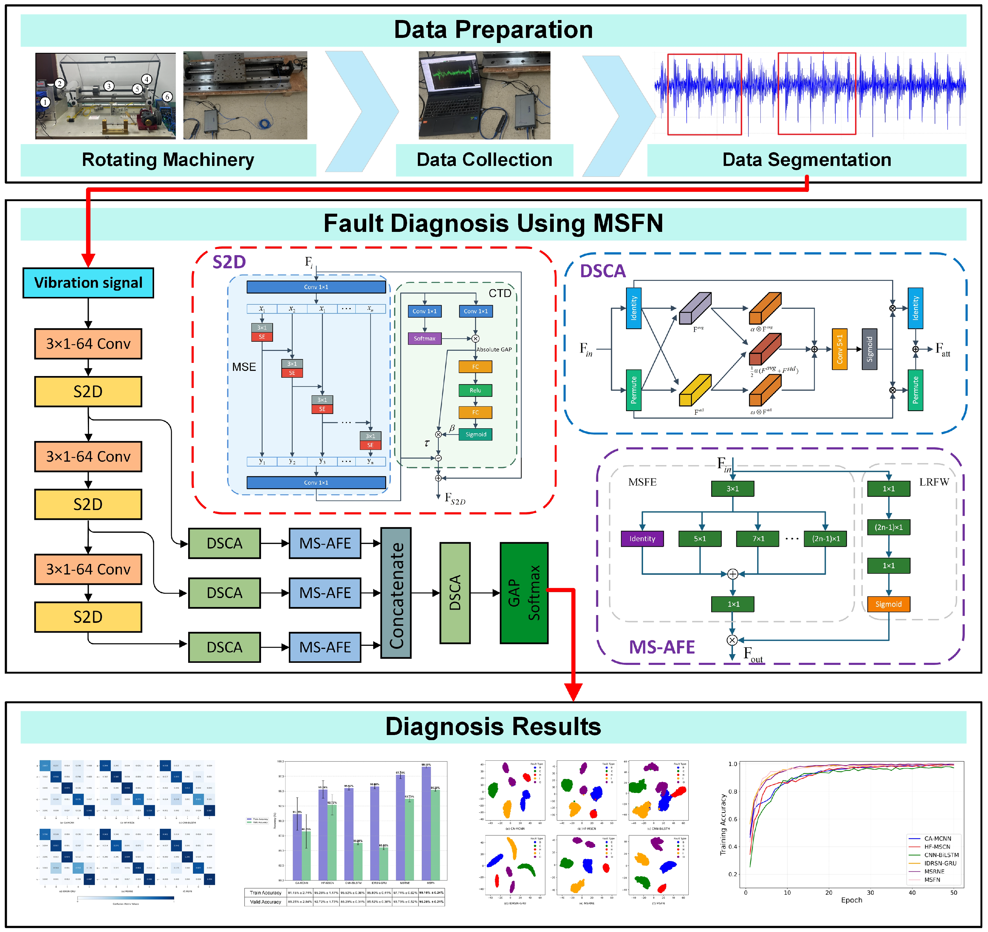
This section provides a systematic description of the architecture and implementation of the proposed MSFN. As depicted in Figure 1, the MSFN consists of convolutional blocks, S2D modules, MS-AFE modules, DSCA modules, a global average pooling (GAP) layer, and a classification layer. The backbone of MSFN, comprising convolutional blocks and S2D modules, extracts comprehensive multi-scale fault features from input vibration signals at multiple levels. Intermediate features from various backbone stages are passed to DSCA modules, which apply collaborative attention across sequence and channel dimensions to amplify fault-relevant information. Subsequently, the MS-AFE module further enhances periodic characteristics using large receptive field weighting. The enhanced feature representations are concatenated along the channel dimension and processed again through the DSCA module for feature fusion, effectively emphasizing critical channels and fault-related information. In the final stage, the fused features undergo a GAP operation before being passed to the classification layer to generate accurate and reliable fault diagnosis results.

2.2. S2D

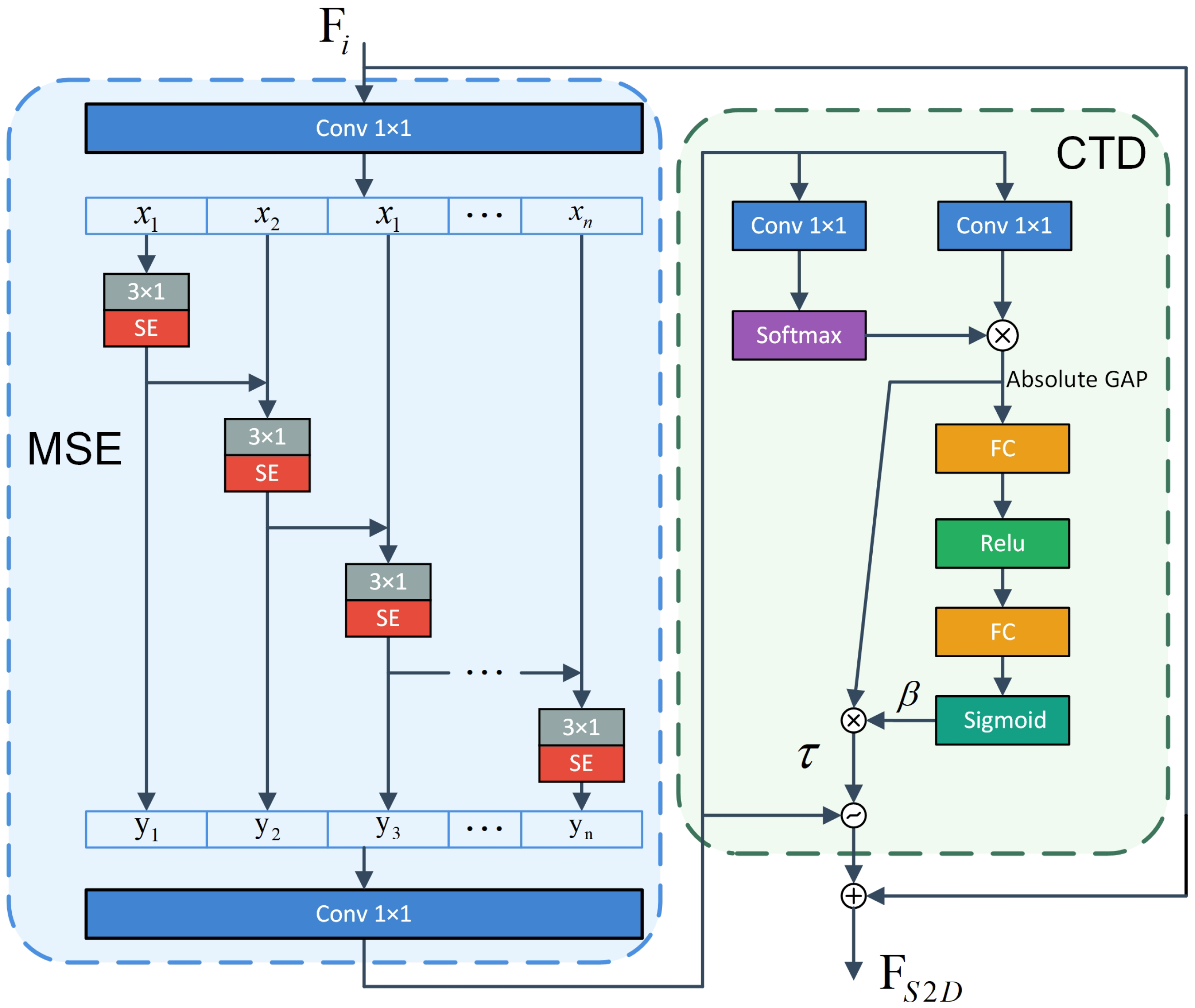
S2D is the core component designed to extract multi-scale fault features from vibration signals while suppressing irrelevant features. It comprises: (1) Multi-Scale Extraction (MSE) with channel attention, for capturing multi-scale features, and (2) channel threshold denoising (CTD), for adaptive noise suppression. Figure 2 illustrates the architecture of S2D.

2.2.1. MSE

Inspired by Res2Net [29], MSE facilitates efficient multi-scale feature learning. Unlike Res2Net, MSE omits the retention of raw features during multi-scale processing and instead introduces additional convolutional branches to broaden receptive fields. Furthermore, each branch integrates a squeeze-and-excitation (SE) attention mechanism to reinforce feature representation.

Given an input feature tensor $F_i\in {\mathbb{R}}^{C\times L}$, MSE applies a series of $1\times 1$ convolutions for dimensional expansion to enhance feature information, yielding the expanded features $F_e\in {\mathbb{R}}^{C_1\times L}$:

$$F_e=Con{v}_{1\times 1}\left(F_i\right)$$

(1)

Subsequently, $F_e$ is evenly split along the channel dimension into n subsets $x_i\in {\mathbb{R}}^{{\displaystyle \frac{C_1}{n}}\times L}$:

$$Split\left(F_e\right)=\{x_1,x_2,\dots ,x_n\}$$

(2)

where $C_1=kn$, k represents the number of channels in each subset $x_i$, and $i=1,2,\dots ,n$. Each $x_i$ is processed by a corresponding feature extraction unit $E_i\left(·\right)$, which consists of $C_2$ convolutional operations with a kernel size of $3\times 1$, followed by an SE module (refer to [30] for SE implementation details, with reduction ratio $r=2$). The outputs $y_i$ of each extraction unit are generated in a hierarchical manner. The first feature extraction unit $E_1\left(·\right)$ processes $x_1$ directly, while the subsequent unit $E_i\left(·\right)$ processes the element-wise sum of the current feature subset $x_i$ and the output of the previous unit $y_{i-1}$:

$$y_i=E_i\left(x_i\right)=\left\{\begin{array}{cc}SE\left({Conv}_{3\times 1}\left(x_i\right)\right),\hfill & i=1,\hfill \\ SE\left({Conv}_{3\times 1}(x_i+y_{i-1})\right),\hfill & 2\le i\le n.\hfill \end{array}\right.$$

(3)

The multi-scale features $y_i$ are concatenated along the channel dimension to form the comprehensive multi-scale representation $F_m$:

$$F_m=Contact\left(y_1,y_2,\dots ,y_n\right)$$

(4)

Finally, MSE applies $C_1$ $1\times 1$ convolutions to adjust the dimensions, generating the multi-scale feature representation $F_{multi}$:

$$F_{multi}={Conv}_{1\times 1}\left(F_m\right)$$

(5)

2.2.2. CTD

The multi-scale features extracted by MSE remain susceptible to noise contamination, which impedes the ability to isolate fault-related patterns with high precision. Therefore, it is essential to suppress interfering features while extracting multi-scale fault features. To achieve this, the CTD module is integrated into the S2D, which employs adaptive channel-wise thresholding to filter interference and increase feature sparsity to enhance generalization performance.

The theoretical foundation of threshold-based feature denoising is based on treating low-magnitude features as potential interference. The thresholding function is defined as follows:

$$F_o\left(F_{multi}\right)=\left\{\begin{array}{cc}{F}_{multi}-\tau ,\hfill & F_{multi}>\tau \hfill \\ 0,\hfill & -\tau \le F_{multi}\le \tau \hfill \\ F_{multi}+\tau ,\hfill & F_{multi}<-\tau \hfill \end{array}\right.$$

(6)

where $F_{multi}$ represents the multi-scale features extracted by MSE, $\tau$ denotes the adaptive noise threshold parameter, and $F_o\left(·\right)$ represents the refined multi-scale features obtained after noise suppression through the thresholding operation. The core of CTD lies in the adaptive determination of this threshold.

The proposed CTD integrates a context-guided mechanism with channel attention to implement adaptive soft-thresholding. Specifically, a $1\times 1$ convolution is applied to $F_{multi}$ to generate context-aware representations. Through this transformation, channels containing noise-related information are identified and weighted accordingly. Subsequently, a channel-wise Softmax operation normalizes these weights, and element-wise multiplication produces the context-modulated feature representation:

$$F_{context}={\mathrm{Conv}}_c\left(F_{multi}\right)\otimes \mathrm{Softmax}\left({\mathrm{Conv}}_c\left(F_{multi}\right)\right)$$

(7)

where $F_{context}$ represents the features containing noise information, and ⊗ denotes the element-wise multiplication. To capture the global statistical properties of the context features, GAP is applied to the absolute values as follows:

$$F_g=\mathrm{GAP}\left(\right|F_{context}\left|\right)$$

(8)

where $GAP\left(·\right)$ represents the global average pooling operation, and $\left|·\right|$ computes element-wise absolute values. The channel-specific noise suppression weights are learned through a two-layer fully connected network with a bottleneck structure as follows:

$$\beta =\rho \left(W_2·\sigma \left(W_1·F_g\right)\right)$$

(9)

where $\sigma$ and $\rho$ denote ReLU and Sigmoid activation functions, respectively. The weight matrices are defined as $W_1\in {\mathbb{R}}^{{\displaystyle \frac{C}{r}}\times C}$ and $W_2\in {\mathbb{R}}^{C\times {\displaystyle \frac{C}{r}}}$, with the reduction ratio set to $r=2$ to lower computational cost. The channel-wise noise threshold $\tau$ is obtained through element-wise multiplication:

$$\tau =F_g\otimes \beta$$

(10)

Finally, to mitigate overfitting within the S2D, a residual connection is introduced between the input $F_i$ and output $F_o$:

$$F_{\mathrm{S}2\mathrm{D}}=F_i+F_o$$

(11)

2.3. MS-AFE

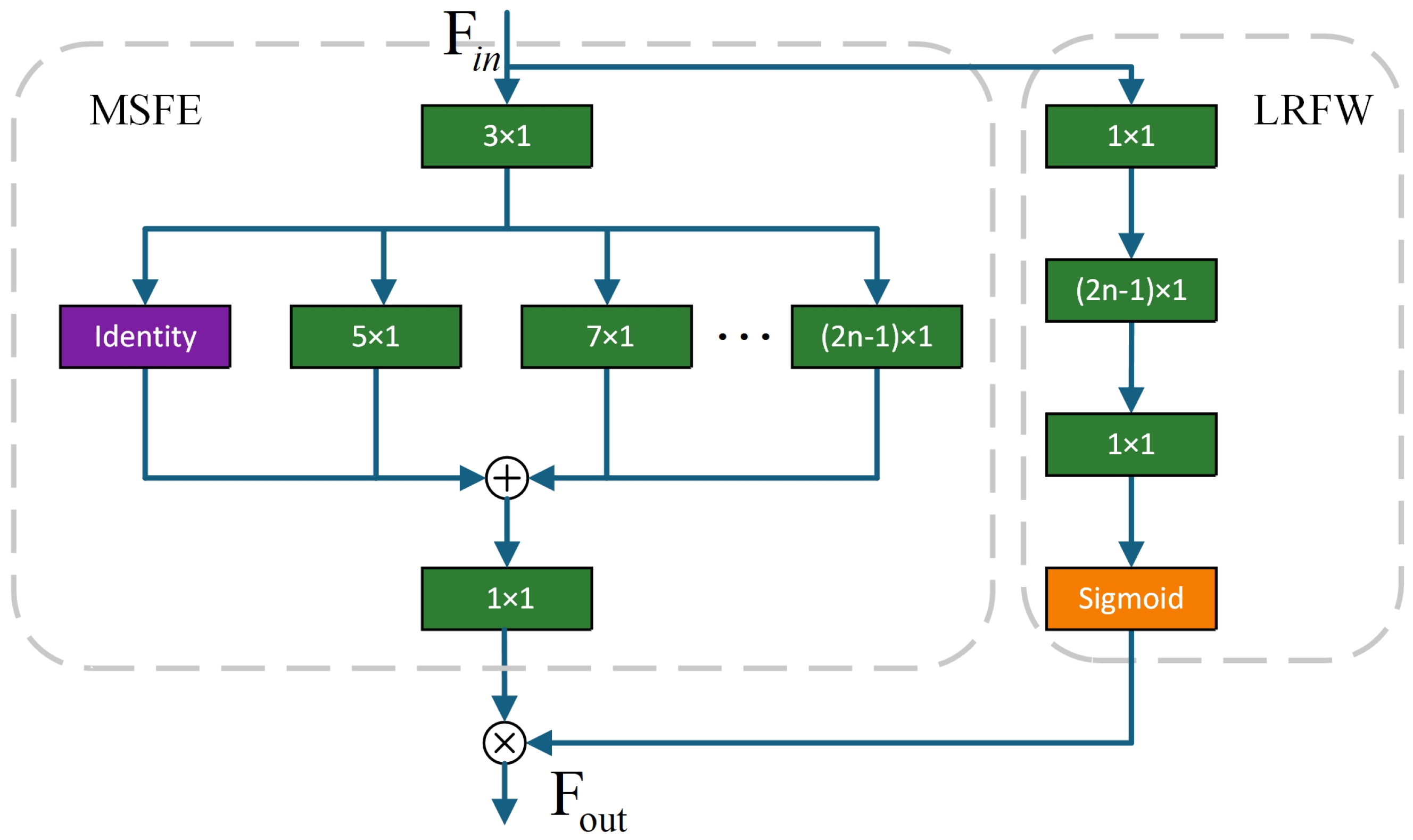
Although S2D incorporates a multi-scale feature mechanism, its representational capacity across various scales remains constrained. Furthermore, mechanical faults often manifest as periodic signatures that require specialized attention mechanisms. Therefore, we introduce the MS-AFE module, which amplifies scale-dependent information and emphasizes periodic patterns. As shown in Figure 3, MS-AFE adopts a dual-branch architecture: the Multi-Scale Feature Enhancement (MSFE) branch and the long-range feature weighting (LRFW) branch.

2.3.1. MSFE

MSFE is inspired by the Inception architecture [31] to enhance multi-scale representation through parallel convolution operations with diverse receptive fields. The branch initially captures fine-grained patterns using a 3 × 1 convolution, subsequently extracting coarser features through $n-1$ parallel branches with incrementally larger kernel sizes:

$$x_i=\left\{\begin{array}{cc}{\mathrm{Conv}}_{3\times 1}\left(F_{in}\right),\hfill & i=1\hfill \\ {\mathrm{Conv}}_{(2i+1)}\left(x_1\right),\hfill & i=2,\dots ,n\hfill \end{array}\right.$$

(12)

where x represents the input feature tensor, $x_1$ denotes the small-scale features captured through $3\times 1$ convolution operations, $x_i$ represents the multi-scale features obtained from the i-th parallel convolution branch, and n indicates the total number of parallel convolution branches in the architecture.

This branch subsequently aggregates features using a 1 × 1 convolution, which integrates fine-scale details with broader contextual information to produce the enhanced multi-scale representation $F_m$:

$$F_m={\mathrm{Conv}}_{1\times 1}\left(\sum _{i=1}^n{x}_i\right)$$

(13)

2.3.2. LRFW

LRFW is designed to enhance periodic information. Initially, a $1\times 1$ convolution mixes the channels:

$$F_c={\mathrm{Conv}}_{1\times 1}\left(F_{in}\right)$$

(14)

where $F_c$ represents the features after information exchange.

Subsequently, a $(2n-1)\times 1$ convolution captures long-range temporal correlations $F_l$:

$$F_l={\mathrm{Conv}}_{(2n-1)\times 1}\left(F_c\right)$$

(15)

Feature fusion is performed through a $1\times 1$ convolution, and long-range attention weights $F_A$ are generated using the Sigmoid activation function:

$$F_A=\mathrm{Sigmoid}\left({\mathrm{Conv}}_{1\times 1}\left(F_l\right)\right)$$

(16)

The final output $F_{out}$ of the MS-AFE module is obtained through element-wise multiplication of the enhanced multi-scale features and adaptive attention weights:

$$F_{out}=F_m\otimes F_A$$

(17)

2.4. DSCA

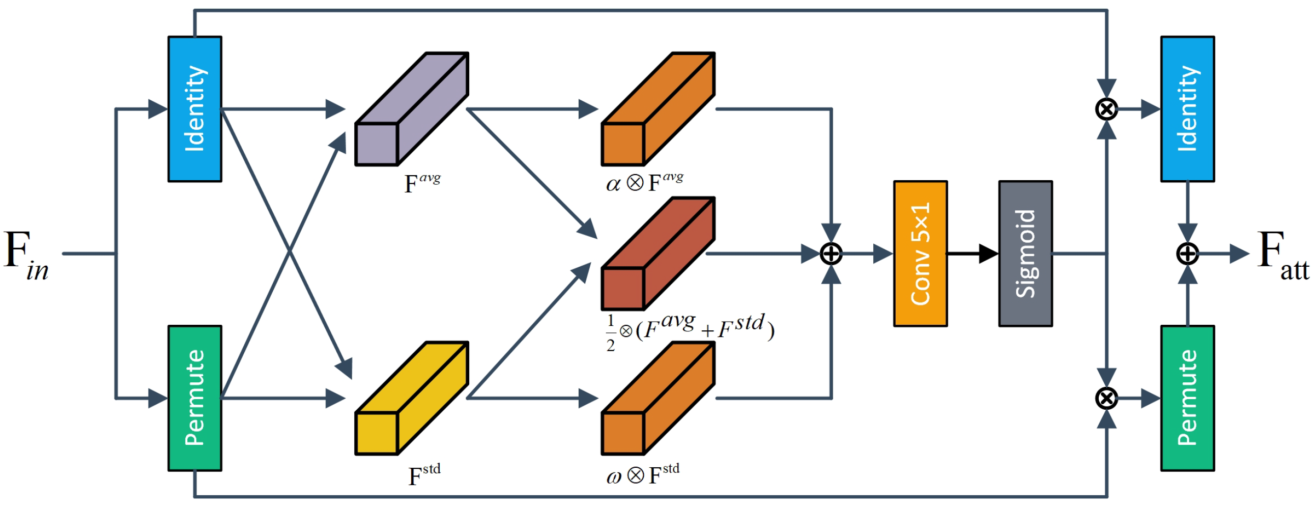
Identification of temporal patterns is essential for achieving high-precision fault detection in rolling bearings. Inspired by Ref. [32], we designed the DSCA module to enhance the ability to capture temporal information and channel-specific features. As shown in Figure 4, DSCA consists of two parallel branches: the upper branch captures inter-channel dependencies, while the lower branch focuses on dependencies along the sequence dimension.

Given an input feature tensor $F_{in}\in {\mathbb{R}}^{C\times L}$, the sequential attention mechanism first applies a permutation operation to restructure the tensor for capturing temporal relationships:

$$F_r=P\left(F_{in}\right)$$

(18)

where $F_{in}$ represents the input feature tensor, $F_r$ denotes the time-dependent features, and P denotes a permutation operation that reshapes the input from ${\mathbb{R}}^{C\times L}$ to ${\mathbb{R}}^{L\times C}$, and $P^{-1}$ represents its inverse operation, used to restore the original dimensions.

After the permutation, AVG and global standard-deviation (STD) pooling are applied to extract overall trends and local variations:

$${\nu }_l^{avg}={\displaystyle \frac{1}{C}}\sum _{i=1}^C{\nu }_l\left(i\right)$$

(19)

$${\nu }_l^{std}=\sqrt{{\displaystyle \frac{1}{C}}\sum _{i=1}^C{\left({\nu }_l\left(i\right)-{\nu }_l^{avg}\right)}^2}$$

(20)

where ${\nu }_l\in {\mathbb{R}}^{C\times 1}$ represents the l-th time step feature vector, ${\nu }_l^{avg}$ represents the overall trend of channel features at the l-th sequence position, and ${\nu }_l^{std}$ denotes the local trend of channel features at the l-th sequence position. The pooled features, denoted as $F^{\mathrm{avg}}=\left[v_1^{\mathrm{avg}},\cdots ,v_L^{avg}\right]$ and $F^{std}=\left[v_1^{std},\cdots ,v_L^{std}\right]$, are fused by a dynamic weighting strategy:

$$F_{sq}={\displaystyle \frac{1}{2}}\otimes \left(F^{avg}\oplus F^{std}\right)\oplus \alpha \otimes F^{avg}\oplus \omega \otimes F^{std}$$

(21)

where $F_{sq}$ represents the dynamically weighted features, and ⊗ and ⊕ denote element-wise multiplication and addition, respectively; $\alpha$ and $\omega$ are learnable parameters updated during backpropagation.

To refine the attention signal, a $5\times 1$ convolutional filter is applied, followed by a Sigmoid activation function that generates the attention weights $W_a$:

$$W_a=Sigmoid\left({Conv}_{5\times 1}\left(F_{sq}\right)\right)$$

(22)

Subsequently, the weights are applied to the permuted features to obtain the sequence-enhanced representation ${\widehat{F}}_{seq}$:

$${\widehat{F}}_{seq}=P^{-1}(W_a\otimes F_r)$$

(23)

In parallel, the channel attention branch applies the same mechanism to the original input tensor $F_{in}$, capturing inter-channel dependencies and producing channel-enhanced features $\widehat{F_c}$.

The final output of DSCA is obtained by averaging the results from the two branches:

$$F_{att}={\displaystyle \frac{1}{2}}\left({\widehat{F}}_{seq}+{\widehat{F}}_c\right)$$

(24)

where $F_{att}$ represents the output features of DSCA.

3. Experiments and Results

This section evaluates the performance of the proposed MSFN using two datasets. In Section 3.1, we utilize the HUST dataset to examine the influence of parameters on model performance and explore the model’s transferability under variable speed conditions. In Section 3.2, we introduce the experimental platform used to simulate feed platform faults, validating the fault diagnosis capability of the model and its transferability across different load conditions.

3.1. Experiments on the HUST Public Dataset

3.1.1. Dataset Description

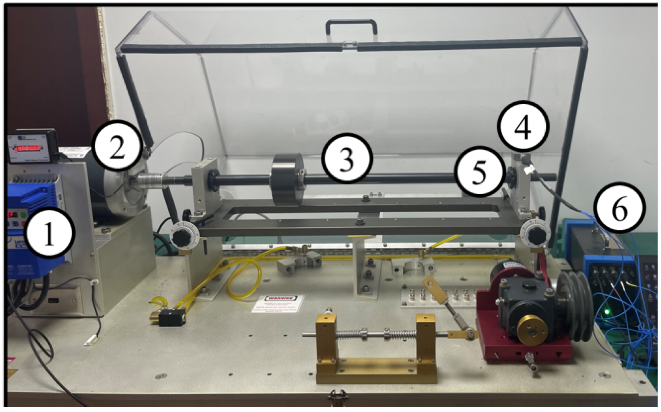
Fault simulation is performed using a rolling bearing fault simulator (Spectra-Quest Inc., Richmond, VA, USA) [33]. The structure of the test rig, illustrated in Figure 5, consists of the following components: (1) a speed controller, (2) a motor, (3) a shaft, (4) an accelerometer, (5) the test bearing, and (6) a data acquisition system. The ER-16K deep groove ball bearings were used in the experiments, with artificial defects introduced into the rolling elements, inner ring, and outer ring through electrical discharge machining. The dataset includes five classes: healthy (H), ball fault (BF), inner-ring fault (IF), outer-ring fault (OF), and combined inner- and outer-ring faults (CFs). Each fault class is divided into moderate and severe degradation levels based on the size of the defects. In this study, data corresponding to different degradation levels of the same fault location are treated as a single fault category. To evaluate robustness against speed variation, six operating conditions were recorded: five at constant speeds (40 Hz, 35 Hz, 30 Hz, 25 Hz, and 20 Hz), and one under acceleration–deceleration (0 → 40 Hz → 0), designated as datasets A through F. Detailed specifications of each dataset are provided in

Table 1. Detailed information of the HUST dataset.

Fault Location		H	RF		IF		OF		CF		Speed
Damage Size (mm)		–	0.25	0.50	0.15	0.30	0.15	0.30	0.15	0.30
Fault Label		0	1		2		3		4
Dataset	A	511	511	511	511	511	511	511	511	511	40 Hz
	B	511	511	511	511	511	511	511	511	511	35 Hz
	C	511	511	511	511	511	511	511	511	511	30 Hz
	D	511	511	511	511	511	511	511	511	511	25 Hz
	E	511	511	511	511	511	511	511	511	511	20 Hz
	F	511	511	511	511	511	511	511	511	511	0→40→0 Hz

. For each condition, 262,144 data points were recorded during the steady-state phase, with a sampling frequency of 25.6 kHz. During the data preprocessing stage, each sample was segmented into 1024 points, with a stride of 512 points. The entire dataset was divided into training, validation, and testing subsets in a 7:2:1 ratio.

3.1.2. Experimental Environment

Experiments were conducted on a Windows 11 platform equipped with an Intel i7-12800HX processor (Intel Corporation, Santa Clara, CA, USA), an NVIDIA GeForce RTX 4070 GPU (NVIDIA Corporation, Santa Clara, CA, USA), and 32 GB of RAM (Micron Technology, Boise, ID, USA). All methods were implemented using Python 3.10.14 and the PyTorch 2.4.0 framework.

3.1.3. Evaluation Metrics

To evaluate the performance of MSFN and the baseline models, accuracy was used as the primary evaluation metric for assessing fault classification performance. The maximum, minimum, and mean accuracies were recorded to assess performance stability. Confusion matrices were employed to examine the classification behavior across different fault categories. To ensure the reliability and objectivity of the results, each model was trained and tested over five iterations to minimize the influence of random initialization.

3.1.4. Model Parameter Selection

To evaluate the performance of MSFN, experiments were conducted to assess the impact of three key parameters in S2D: the dimension expansion factor $C_1$, the number of multi-scale branches n, and the filter capacity $C_2$, as well as the number of multi-scale branches n in MS-AFE. Model parameters, batch inference time, and model accuracy were selected as evaluation metrics. In the experiment, the batch size was set to 32, and the learning rate was fixed at 0.001.

(1)

Effect of the Dimension Expansion Factor on Model Performance

To evaluate the impact of $C_1$ on the feature representation capability and computational efficiency, experiments were conducted with $n=4$ and $C_2=64$ fixed, while varying $C_1$ among 8, 16, 32, and 64. The model performance for each setting is summarized in

Table 2. Effect of $C_1$ on model complexity, latency, and accuracy.

${\mathit{C}}_1$	Model Parameters	Inference Time (ms)	Accuracy (%)
8	56,133	6.78	92.59
16	128,949	7.73	94.69
32	405,333	8.29	96.93
64	1,481,109	13.91	98.51

.

The results indicate that increasing $C_1$ consistently improves classification accuracy, rising from 92.59% to 98.91%. This enhancement can be attributed to the higher-dimensional feature space afforded by larger $C_1$ values, which allows the network to extract more informative features, thereby strengthening its discriminative capability. However, this improvement is accompanied by a substantial increase in computational cost. When $C_1$ is raised from 32 to 64, the number of model parameters increases from 405,333 to 1,481,109, and the inference time increases from 8.29 ms to 13.91 ms. Taking accuracy and computational efficiency into account, $C_1=32$ is identified as the optimal configuration for MSFN.

(2)

Effect of the Number of Multi-Scale Branches on Model Performance

The parameter n determines the depth of multi-scale feature extraction and the number of processing paths in MSFN, directly influencing the model’s capacity to detect fault patterns across different temporal scales. To equalize representational capacity across branches, we set $C_1=4n$ and fix $C_2=64$. Four configurations were evaluated— $(C_1=8,n=2)$, $(C_1=16,n=4)$, $(C_1=32,n=8)$, and $(C_1=64,n=16)$—and their results are summarized in

Table 3. Effect of n on model complexity, latency, and accuracy.

Configuration	Model Parameters	Inference Time (ms)	Accuracy (%)
${\displaystyle C_1=8,n=2}$	80,709	6.83	91.64
${\displaystyle C_1=16,n=4}$	128,949	7.78	95.29
${\displaystyle C_1=32,n=8}$	393,045	8.04	99.24
${\displaystyle C_1=64,n=16}$	1,462,677	47.35	99.51

.

As shown in Table 3, accuracy increases monotonically, rising from 91.64% to 99.51% as n expands from 2 to 16. These improvements confirm that additional processing paths enhance the ability to capture multi-scale features. However, the relationship between model complexity and performance shows diminishing marginal returns. When n increases from 8 to 16, accuracy improves by only 0.27%, while computational demands escalate significantly—the parameter count rises from 393,045 to 1,462,677, and inference time increases from 8.04 ms to 47.35 ms. Based on this cost–benefit analysis, we select $n=8$ as the optimal configuration for MSFN.

(3)

Effect of Filter Capacity on Model Performance

The parameter $C_2$ determines MSFN’s feature mapping capability. To evaluate its effect on diagnostic performance, we fixed $n=8$ and $C_1=32$, and evaluated four settings of $C_2$: 16, 32, 64, and 128. The results are summarized in

Table 4. Effect of $C_2$ on model complexity, latency, and accuracy.

${\mathit{C}}_2$	Model Parameters	Inference Time (ms)	Accuracy (%)
16	361,365	7.34	93.63
32	370,389	7.43	95.68
64	393,045	8.05	99.18
128	456,789	10.73	97.31

.

As $C_2$ increases from 16 to 64, accuracy improves from 93.63% to 99.18%, indicating that a larger filter set provides a richer feature space. However, further increasing $C_2$ to 128 reduces accuracy to 97.31%, suggesting feature redundancy and overfitting. Notably, raising $C_2$ from 16 to 64 increases the parameter count only from 361,365 to 393,045 and the inference time from 7.34 ms to 8.05 ms. Balancing diagnostic accuracy and efficiency, we select $C_2=64$ as the optimal setting for MSFN.

(4)

Effect of Multi-Scale Branches in MS-AFE on Model Performance

The multi-scale branch n in MS-AFE affects the multi-scale feature extraction capability and the effectiveness of long-range feature weighting. To investigate the optimal value of n, we conducted comparative experiments.

Experimental results indicate that the multi-scale branch n plays a crucial role in the feature extraction capability and efficacy of long-range feature weighting. As shown in

Table 5. Effect of n on model complexity, latency, and accuracy.

n	Model Parameters	Inference Time (ms)	Accuracy (%)
3	245,025	7.61	97.02
4	312,981	7.93	97.54
5	393,045	8.05	99.60
6	485,397	10.24	99.75

, when n increases from 3 to 6, the accuracy increases from 97.02% to 99.75%. This improvement highlights the ability to capture fault features on various time scales. Increasing n expands the receptive field, enabling more comprehensive extraction of periodic fault features. However, the improvement comes at a substantial computational cost. Specifically, when n is raised from 3 to 6, the inference time increases from 7.61 ms to 10.24 ms. Moreover, the parameter count nearly doubles, from 245,025 to 485,397, which increases memory requirements and constrains deployment in resource—limited industrial settings. Based on a cost–benefit analysis, we chose $n=5$ as the optimal configuration for MS-AFE.

3.1.5. Training Parameter Selection

MSFN was trained for 50 epochs using the Adam optimizer and cross-entropy loss. To identify the optimal training configuration, we investigated the impact of different combinations of learning rate (LR) and batch size (BS) on training performance.

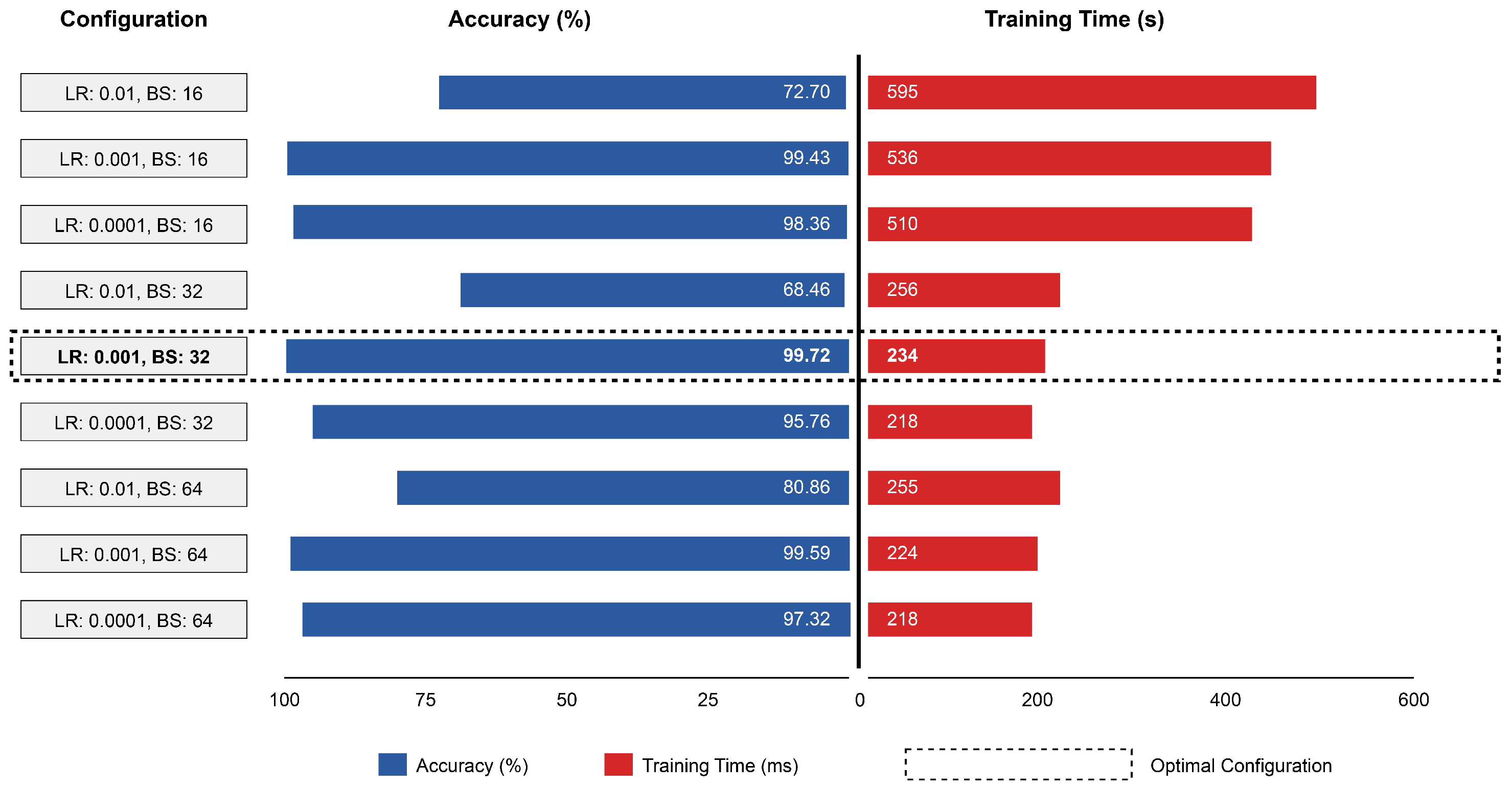
Figure 6 summarizes the accuracy and training time for each LR–BS combination. The LR strongly affects accuracy. With LR = 0.01, the network exhibits poor convergence, and accuracy remains below 80%. Reducing LR to 0.001 improves convergence, with accuracy exceeding 99%. Further reducing LR to 0.0001, however, causes accuracy to decline, indicating underfitting due to slow optimization. The BS primarily affects computational efficiency. Increasing BS from 16 to 32 nearly halves the training time, whereas a further increase to 64 yields only marginal additional savings. Balancing these observations, we select LR = 0.001 and BS = 32 as the optimal configuration.

3.1.6. Comparative Experiments and Results

We compared the performance of the proposed MSFN with five recently published fault diagnosis models: CNN-BiLSTM [34], IDRSN-GRU [35], HF-MSCN [36], CA-MCNN [37], and MSRNE [38]. Each model was trained with its originally published implementation. Experiments were conducted on Dataset A to evaluate the ability of each model to capture common fault features across various fault severity levels.

Table 6. Performance comparison of different models.

Model	Max Accuracy (%)	Min Accuracy (%)	Average Accuracy (%)
CA-MCNN	97.11	95.78	96.68 ± 0.48
HF-MSCN	97.78	94.00	95.49 ± 1.53
CNN-BiLSTM	97.56	96.89	97.22 ± 0.33
IDRSN-GRU	97.33	96.22	96.84 ± 0.39
MSRNE	99.33	98.00	99.09 ± 0.58
MSFN	99.78	99.33	99.60 ± 0.19

summarizes the performance comparison between the proposed MSFN and the five baseline models. MSFN achieves an average classification accuracy of 99.60%, outperforming all baseline models. The second-best performing model, MSRNE, reaches 99.09%, trailing MSFN by 0.51%. In addition to high accuracy, MSFN also demonstrates exceptional stability, with a standard deviation of only ±0.19%. By contrast, CNN-BiLSTM recorded a deviation of ±0.33%, while the other models showed even greater variability. These results demonstrate that MSFN provides stable and reliable diagnostic performance.

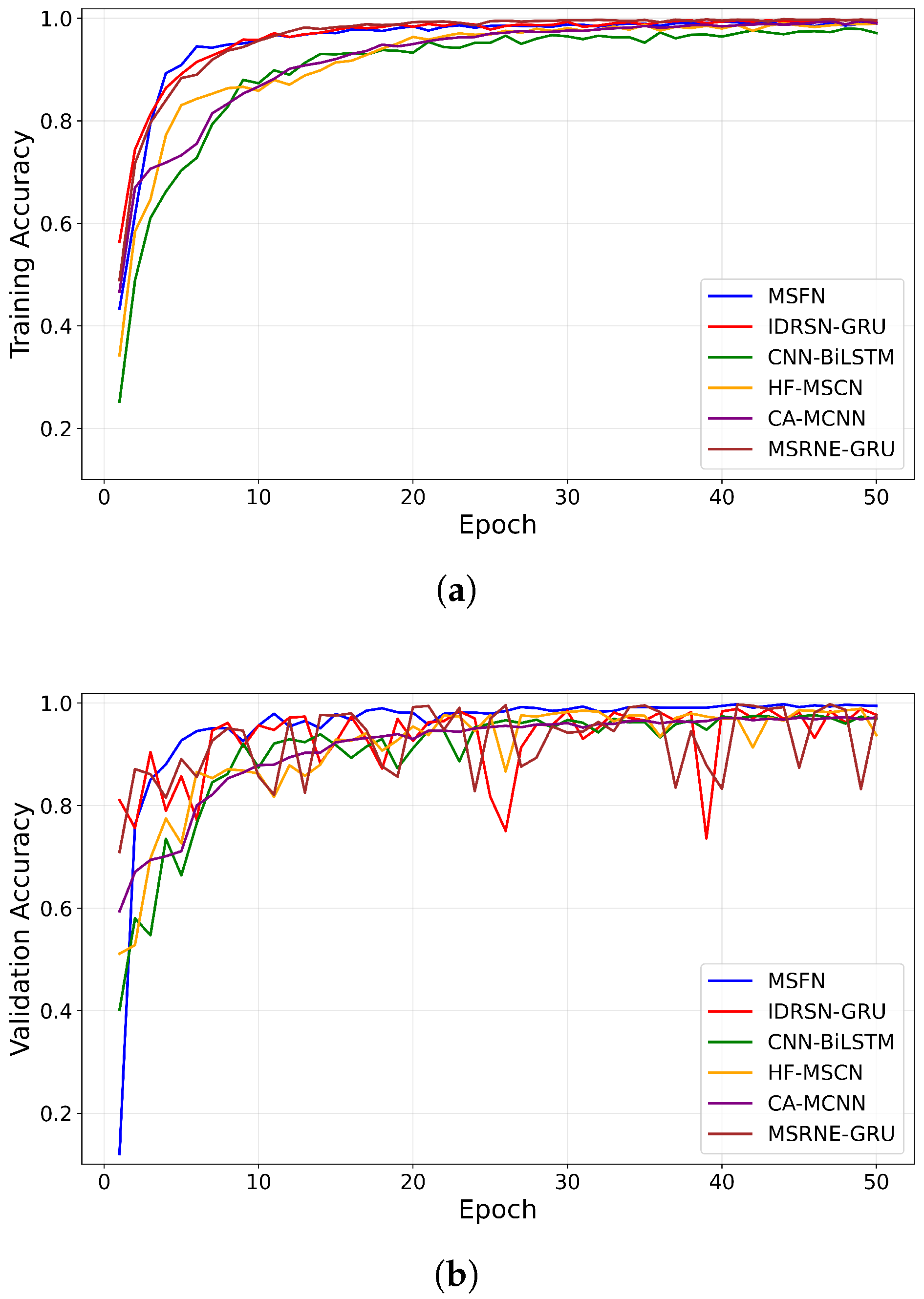
Figure 7 compares the training and validation accuracies of MSFN with five baseline models. From the training curves in Figure 7a, MSFN exhibits superior learning efficiency, exceeding 90% accuracy within five epochs and reaching 99% by epoch 20. The baseline models converge more slowly. Although CNN-BiLSTM, CA-MCNN, and HF-MSCN eventually approach 99% training accuracy, they require more epochs to reach that point. The validation curves in Figure 7b reveal corresponding differences in generalization. MSFN attains 95% validation accuracy by epoch 10 and stabilizes near 99%, with the train-validation discrepancy consistently under 1%. By contrast, IDRSN-GRU and MSRNE exhibit pronounced oscillations in validation accuracy, indicating overfitting and reduced generalization reliability. Although the CA-MCNN validation curve is smoother, a four-percentage-point deficit relative to training accuracy suggests overfitting and limited generalization.

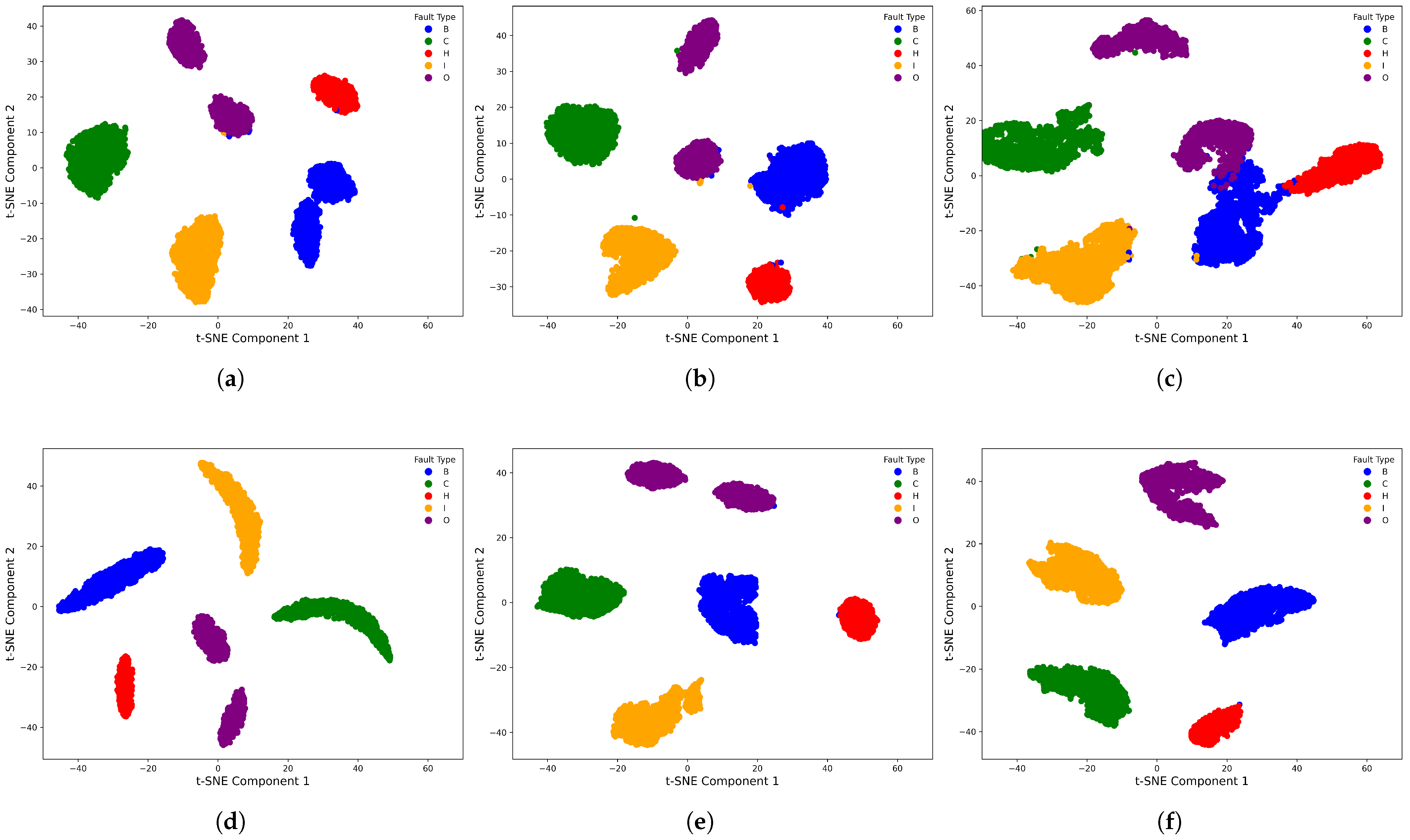
Figure 8 illustrates the t-SNE-based feature visualization for MSFN and the five baseline models. As shown in Figure 8f, MSFN achieves superior fault-feature extraction, with distinctly separated fault categories and compact within-class clusters. This well-structured distribution suggests that MSFN captures shared representations across different damage levels. In contrast, the baseline models exhibit marked shortcomings in capturing inner-race fault features. As shown in Figure 8a–e, these models fail to extract shared inner-race fault features across severity levels, yielding fragmented clusters in feature space. This lack of cohesion indicates limited generalization across fault severities. Moreover, CNN-BiLSTM (Figure 8c) shows overlap between rolling element faults and healthy conditions, which compromises diagnostic reliability.

3.1.7. Variable-Speed Performance

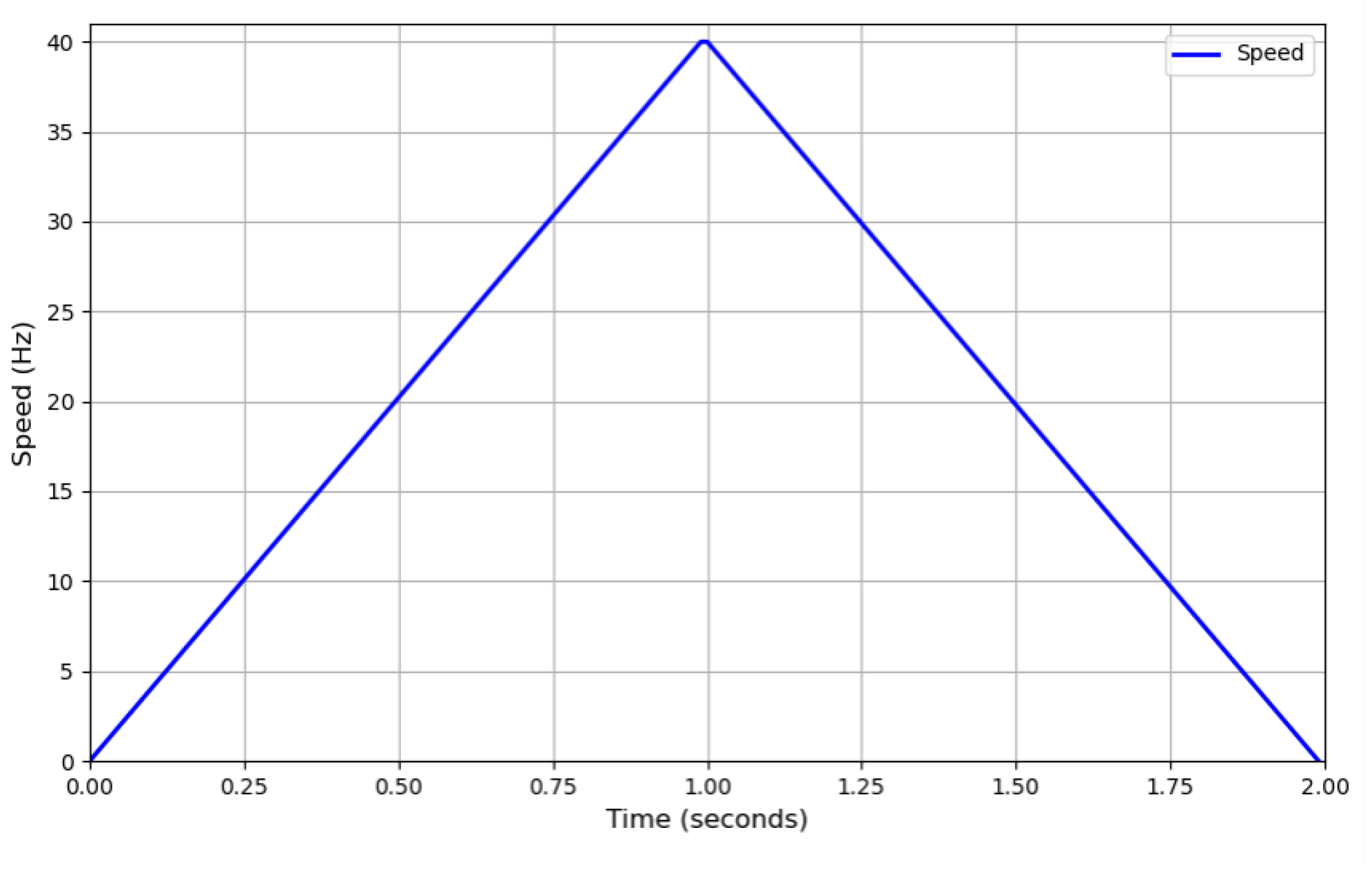
To assess generalization to speed variability, we trained MSFN at a fixed speed and tested it across variable speed. The model was trained on fixed-speed datasets A-E and evaluated on the variable-speed dataset F to assess diagnostic performance under unfamiliar operating conditions. As illustrated in Figure 9, the rotational speed profile of dataset F increases from 0 Hz to 40 Hz within the first second, then decelerates back to 0 Hz, simulating the acceleration and deceleration phases encountered during machinery operation.

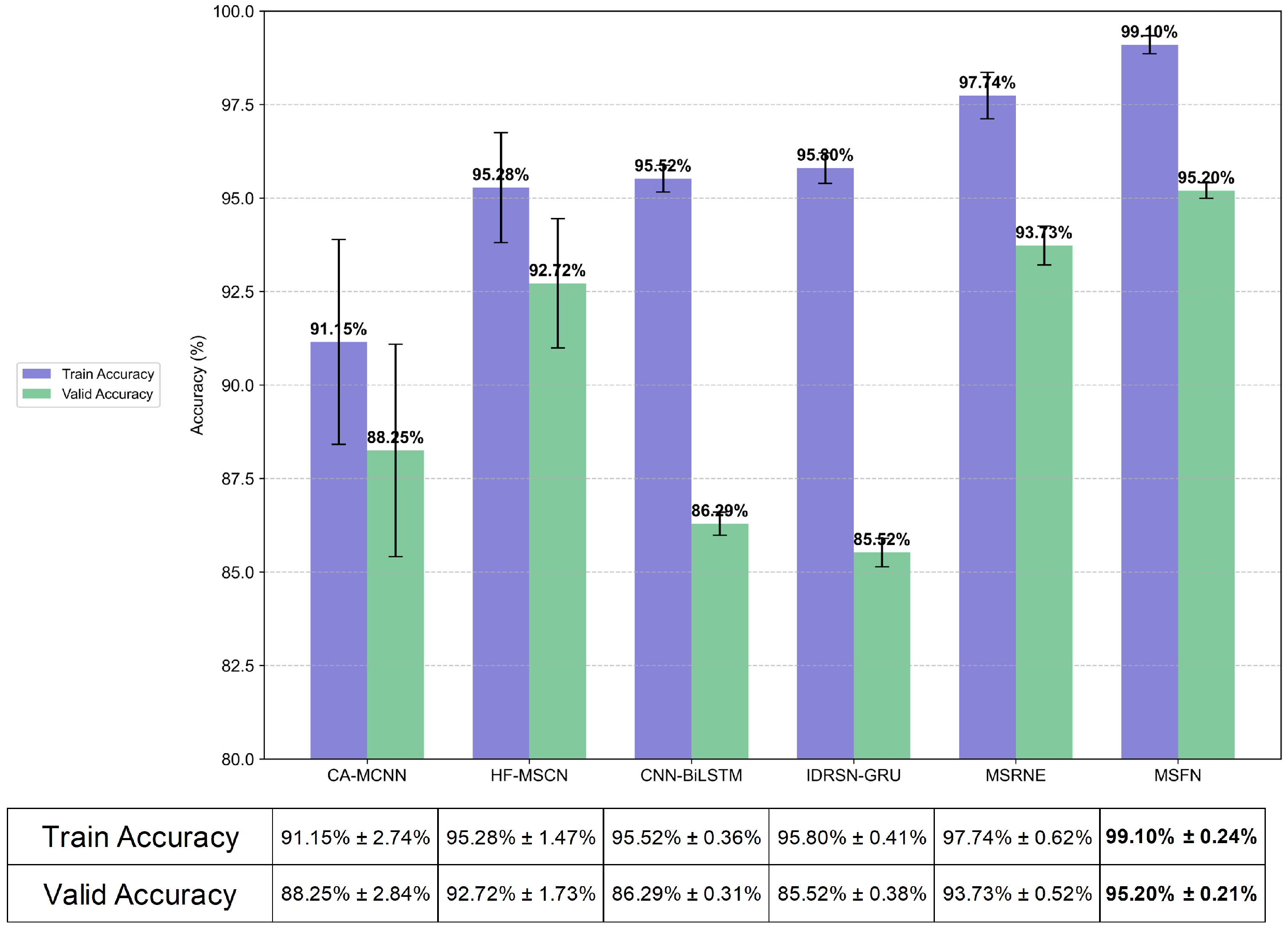
Figure 10 provides a comparative analysis of MSFN and the baseline models on fixed-speed training datasets and a variable-speed test dataset. Under fixed-speed conditions, MSFN outperforms all baselines, achieving an average classification accuracy of 99.10% ± 0.24%. The next best model, MSRNE, achieves 97.74% ± 0.62%, followed by IDRSN-GRU (95.80% ± 0.41%), CNN-BiLSTM (95.52% ± 0.36%), HF-MSCN (95.28% ± 1.47%), and CA-MCNN (91.15% ± 2.74%). On the variable-speed Dataset F, MSFN maintains strong generalization, achieving a classification accuracy of 95.20%. For comparison, MSRNE and HF-MSCN reach 93.73% and 92.72%, respectively, whereas CNN-BiLSTM and IDRSN-GRU achieve 86.29% and 85.52%.

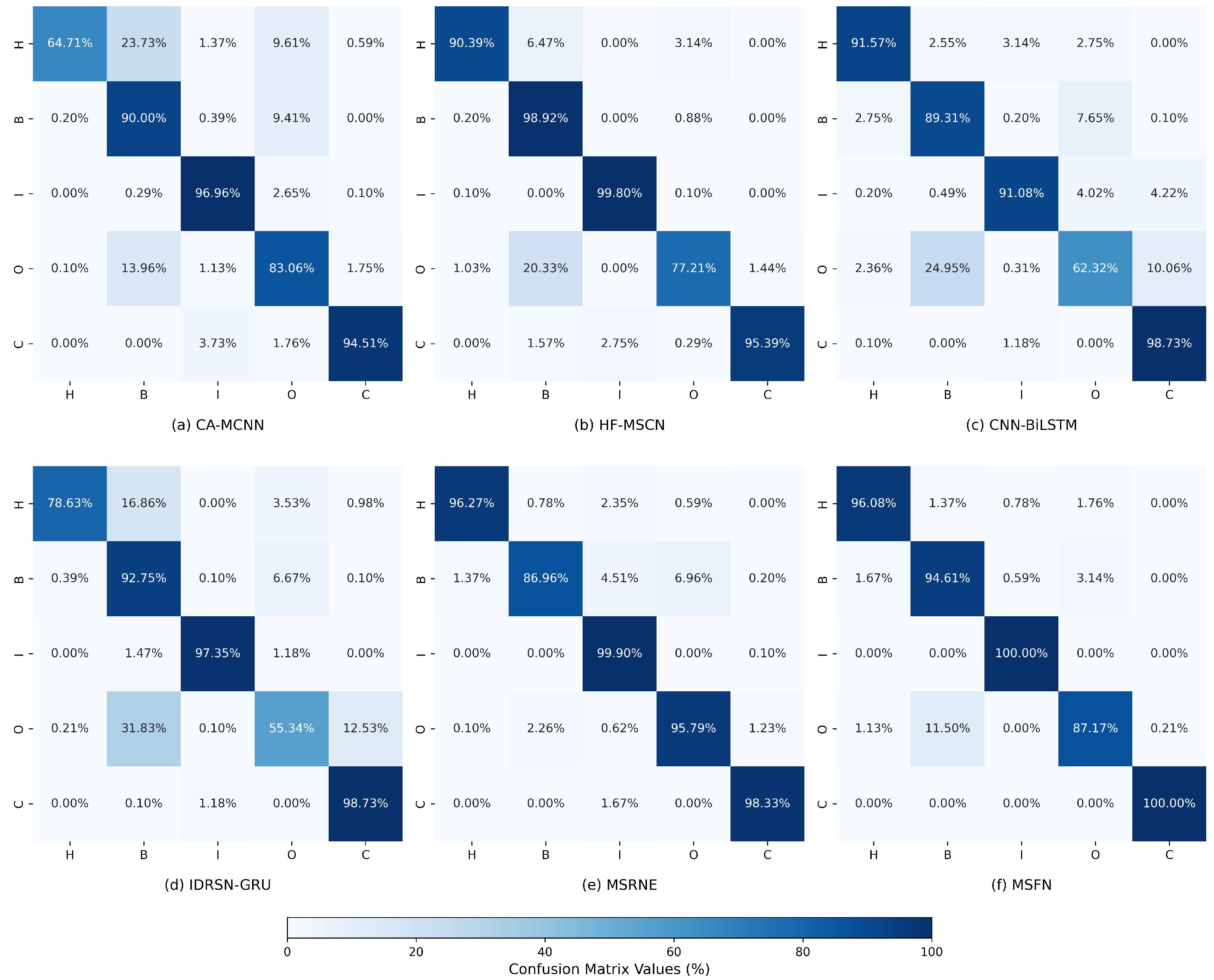
Classification performance under variable-speed conditions was evaluated using confusion matrices for MSFN and the baseline models (Figure 11). MSFN exhibits high diagnostic accuracy across all fault categories, achieving 100% accuracy in identifying inner-race and compound faults. It also performed well on the healthy class and rolling element faults, achieving accuracies of 96.1% and 94.6%, respectively. The only comparatively weaker result occurred for outer-race faults, with an accuracy of 87.2%. In contrast, the baseline models—IDRSN-GRU, CNN-BiLSTM, and HF-MSCN—achieve lower accuracies on outer-race faults (55.3%, 62.3%, and 77.2%, respectively). A large portion of these samples are misclassified as rolling element or compound faults. Additionally, CA-MCNN showed limited reliability on the healthy class, achieving only 84.7% accuracy, with 15% of healthy samples misclassified as rolling element faults.

3.1.8. Ablation Analysis

To evaluate the contributions of each submodule within MSFN to diagnostic accuracy and cross-condition generalization capability, six ablation experiments were designed as follows:

• MSFN: The complete multi-scale feature network, serving as the baseline.
• MSFN-R: Replacing MSE in S2D with the original Res2Net structure.
• MSFN-N: Removing CTD from S2D.
• MSFN-L: Removing the LRFW branch from MS-AFE.
• MSFN-D: Removing the dynamic weight fusion mechanism from DSCA and adopting static weighted fusion for sequence and channel attention.
• MSFN-C: Replacing DSCA with a one-dimensional Convolutional Block Attention Module (CBAM).

Experiments were conducted on the HUST dataset, utilizing conditions A–E to assess the impact of architectural variations on fault recognition performance, while condition F was used to test the transfer capability to unseen speeds. The performance comparison of each ablation model is summarized in

Table 7. Ablation study results of MSFN components.

Module	Diagnosis Accuracy (%)	Change in Diagnosis Accuracy (%)	Transfer Accuracy (%)	Change in Transfer Accuracy (%)	Module Parameters
MSFN	99.10 ± 0.62	-	95.20 ± 0.52	-	393,045
MSFN-R	98.62 ± 0.32	−0.48	92.60 ± 0.29	−2.60	387,445
MSFN-N	98.51 ± 1.05	−0.59	91.53 ± 0.29	−3.67	371,797
MSFN-L	96.63 ± 0.62	−2.47	88.84 ± 0.57	−6.36	312,277
MSFN-D	97.75 ± 0.46	−1.35	91.25 ± 0.62	−3.95	393,029
MSFN-C	97.79 ± 0.52	−1.31	92.41 ± 0.43	−2.79	394,019

.

The results demonstrate that the full MSFN architecture outperforms all ablation variants in both diagnostic accuracy (99.10% ± 0.62%) and transfer accuracy (95.20% ± 0.52%), underscoring the effectiveness of the proposed multi-module collaborative architecture. The replacement of MSE with Res2Net (MSFN-R) resulted in performance degradation of 0.48% and 2.60% for diagnostic and transfer accuracy, respectively. This performance gap underscores the advantage of MSE’s innovative design, which discards original feature information while incorporating additional convolutional branches to more effectively capture multi-scale receptive fields. The removal of CTD (MSFN-N) yielded a notable impact on model stability and generalization. Diagnostic accuracy decreased by 0.59%, while transfer accuracy dropped by 3.67%, accompanied by increased performance variance (standard deviation rising from 0.62% to 1.05%). These findings highlight CTD’s critical role in suppressing irrelevant features and improving robustness across varying operational conditions. Among all ablation variants, the elimination of the LRFW branch (MSFN-L) produced the most substantial performance degradation. Diagnostic accuracy declined by 2.47%, and transfer accuracy experienced a marked reduction of 6.36%. This impact confirms the crucial contribution of the long-range feature weighting mechanism in capturing and reinforcing periodic fault features in sequence contexts. The ablation study of DSCA reveals the superiority of the dynamic dual-dimensional attention mechanism. The removal of the adaptive fusion strategy (MSFN-D) led to reductions of 1.35% and 3.95% in diagnostic and transfer accuracy, respectively, demonstrating that the dynamic weight allocation between sequence and channel attention is crucial for adapting to varying operational conditions. Furthermore, the substitution of DSCA with CBAM (MSFN-C) resulted in performance decreases of 1.31% and 2.79% for diagnostic and transfer accuracy, despite a marginal increase in model parameters (394,019). This performance gap can be attributed to CBAM’s sequential processing architecture, which processes sequence and channel features one after the other, causing information distortion in the sequential domain. In contrast, DSCA uses a parallel processing strategy, allowing both sequence and channel attention branches to operate simultaneously, thus preserving the integrity of both feature domains during the attention computation process.

3.1.9. Feature Visualization and Analysis

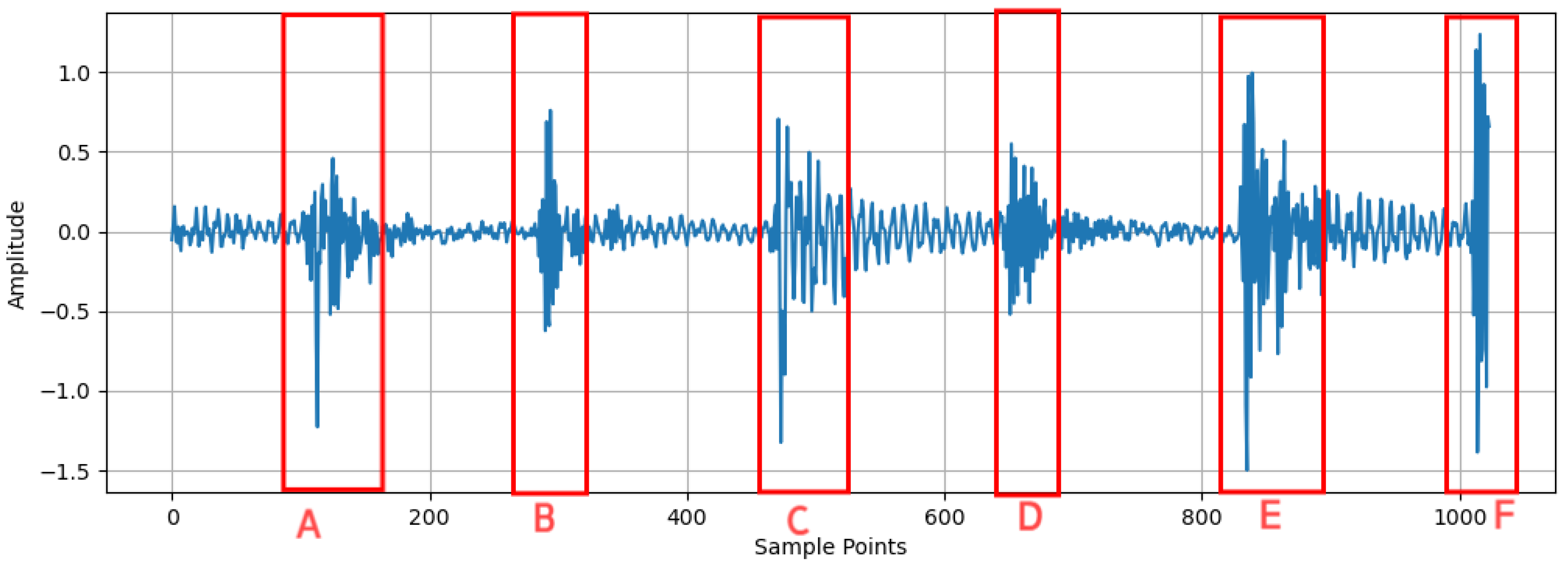
This study visualizes the output features from the core modules of MSFN to explore the feature extraction mechanism and enhance interpretability. A sample is randomly selected from the dataset and fed into MSFN trained as described in Section 3.1.6. Subsequently, the intermediate outputs from submodules are extracted to trace the progression of feature representations throughout the network. As shown in Figure 12, the time-domain waveform of the selected sample corresponds to a bearing with an outer-race fault operating at 40 Hz. This signal exhibits six distinct fault-induced impact pulses, labeled A through F.

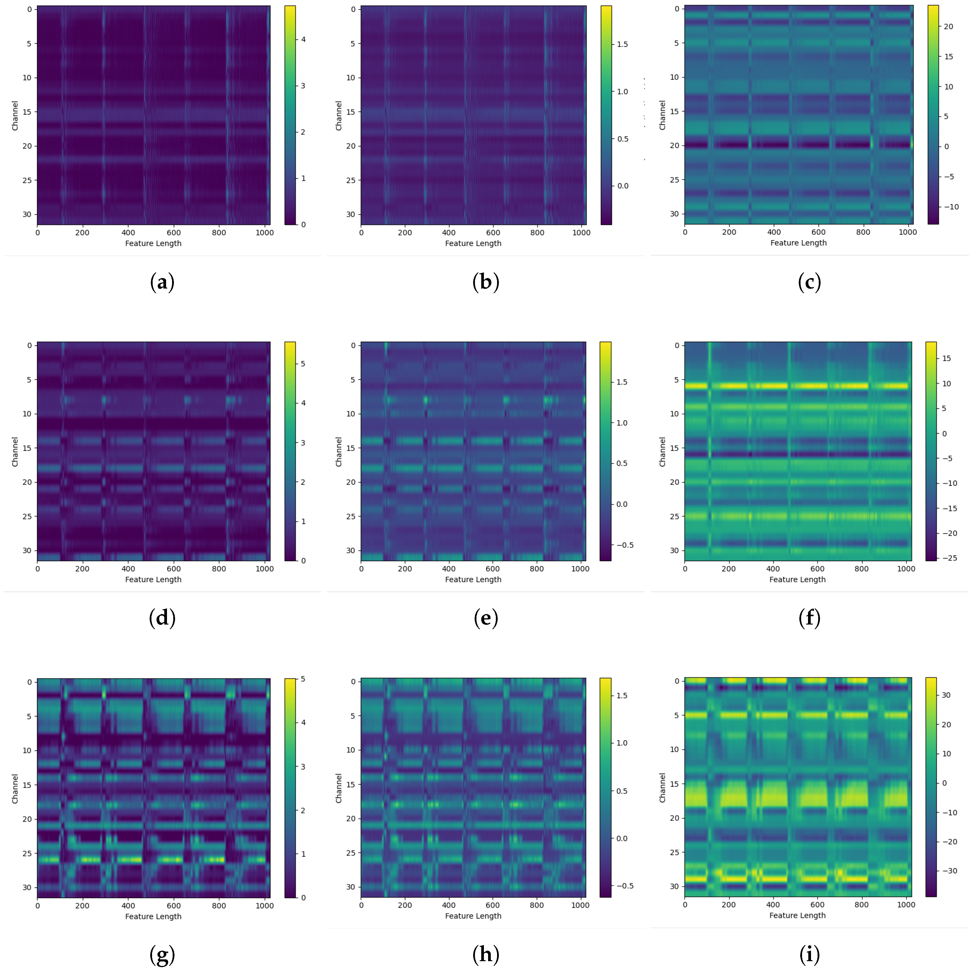
Figure 13 illustrates the feature learning process of MSFN through a heatmap visualization. During the feature extraction phase of the backbone network, S2D produces relatively sparse feature maps (Figure 13a,d), where fault-related features are weakly expressed and lack distinct representation. At this stage, MSFN focuses on extracting low-level spatial features and progressively enlarging the receptive field. As the network deepens, the extracted features become increasingly informative and discriminative. For instance, in the output of the third S2D (Figure 13g), inter-channel variations are more pronounced, indicating enhanced discrimination of critical fault patterns. The incorporation of DSCA (Figure 13b,e,h) further enhances local activation within the feature maps. This enhancement emphasizes fault-relevant features. Subsequently, MS-AFN (Figure 13c,f,i) further strengthens the discriminative capacity of the feature representations. The resulting feature maps display more coherent and structured distributions, with fault-related elements consistently emphasized across channels. This visualization of feature evolution enhances interpretability and provides empirical evidence for the validity and effectiveness of the proposed MSFN in fault-feature extraction.

3.2. Validation on the Self-Built Platform

3.2.1. Dataset Description

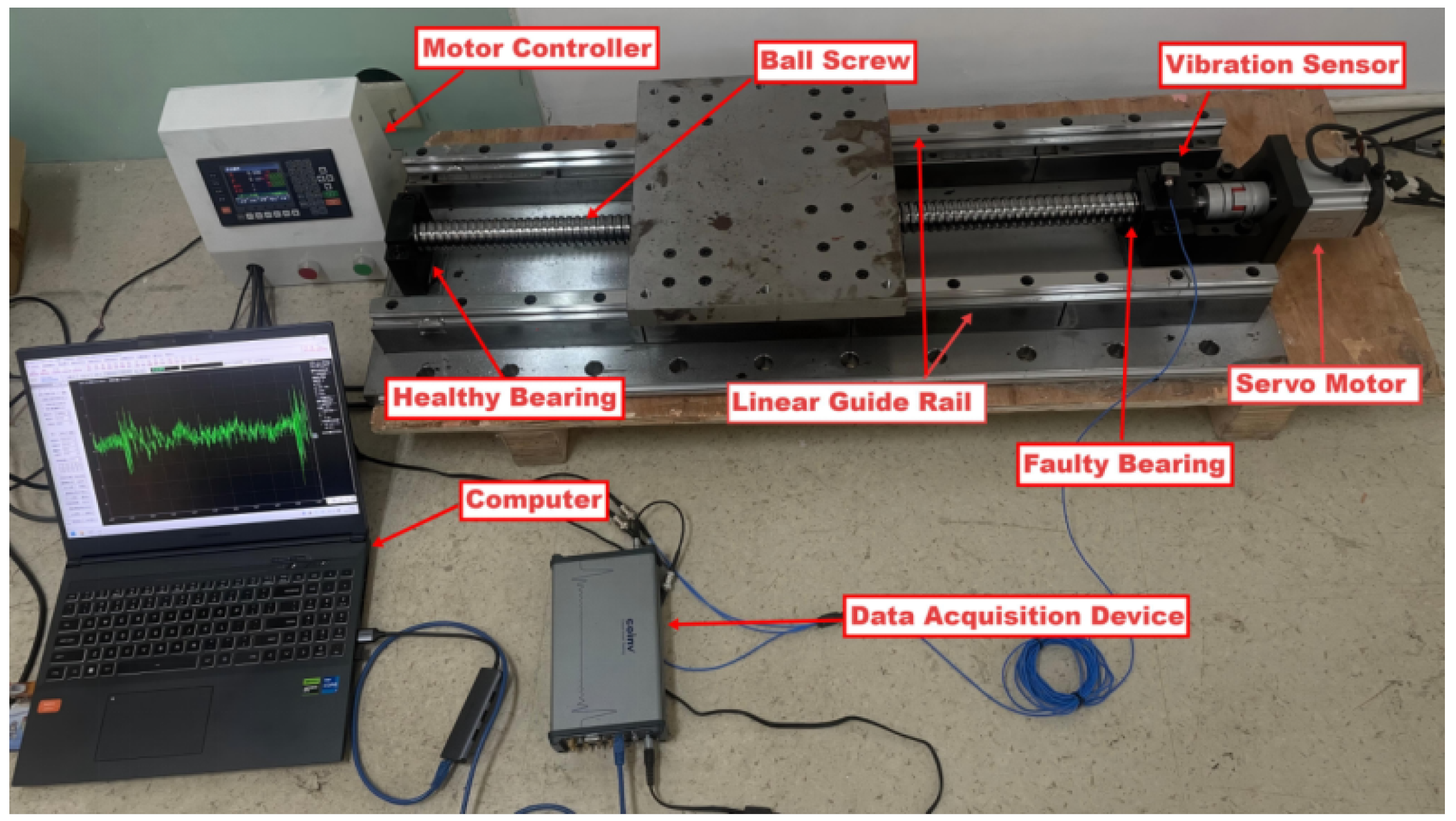
The experimental feed platform, shown in Figure 14, comprises a sliding guide rail, ball screw, servo motor with controller, rolling bearings, vibration sensors, data acquisition device, and a host computer. The support end uses a deep-groove ball bearing (6205), while the drive end is fitted with a pair of angular-contact ball bearings (HRB 7025). To simulate early fatigue spalling, 1 mm wide rectangular notches were introduced into the inner ring, outer ring, or both rings of the drive-end bearings using wire electrical discharge machining. This process defined four health conditions: healthy (H), inner-ring fault (IF), outer-ring fault (OF), and combined inner–outer-ring fault (CF) (see Figure 15).

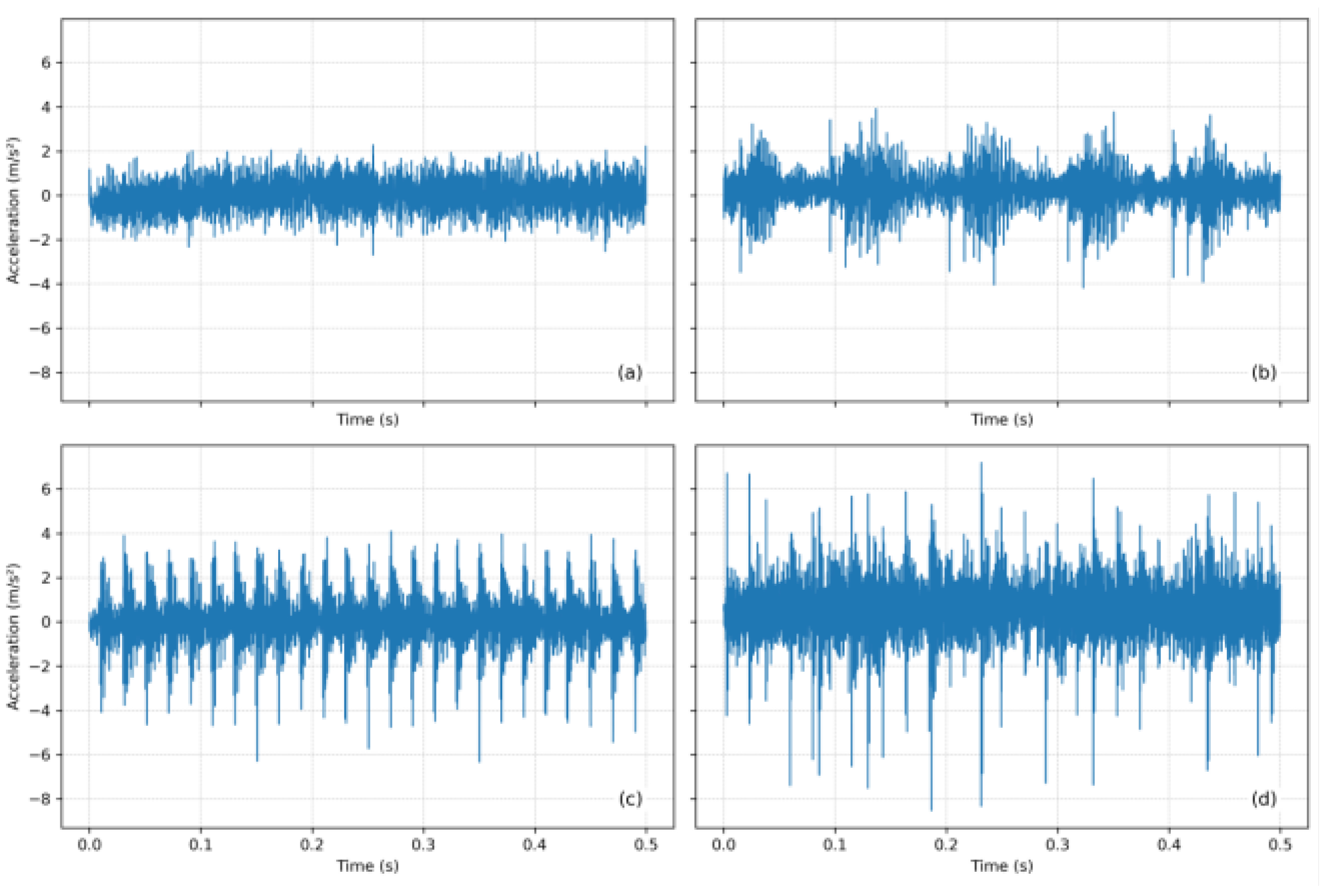
Experiments were conducted under three radial loads (18 kg, 19 kg, and 20 kg) at a constant rotational speed of 600 rpm. Vibration sensors were mounted on the drive-end bearing housing to capture dynamic signals. In each run, the ball-screw actuator traversed a 550 mm stroke: the initial 25 mm and final 25 mm were allocated to acceleration and deceleration, respectively, and the central 500 mm was used for analysis. Figure 16 show time-waveforms recorded from HRB 7025 under the four health conditions. Signals were sampled at 10 kHz, yielding 50,000 points per run. For each fault type, ten replicates were obtained by varying the initial defect location. The signal was segmented into overlapping windows of 2048 points with a step of 1024 samples. The entire dataset was randomly divided into training, validation, and test subsets in a 7:2:1 ratio. Detailed datasets are presented in

Table 8. Dataset details.

	Bearing Condition
	Healthy	Inner Ring	Outer Ring	Inner Ring + Outer Ring	Load (kg)
Label	0	1	2	3
Dataset A	470	470	470	470	18
Dataset B	470	470	470	470	19
Dataset C	470	470	470	470	20

.

3.2.2. Comparative Experiment

To validate the diagnostic capability of MSFN in the feed system, we conducted a comparative evaluation on dataset A.

Table 9. Performance comparison of various models on progressive platform dataset.

Model Name	Max Accuracy (%)	Min Accuracy (%)	Average Accuracy
CA-MCNN	98.40	97.07	97.71 ± 0.52
HF-MSCN	97.94	96.28	97.34 ± 1.08
CNN-BiLSTM	97.87	96.81	97.18 ± 0.45
IDRSN-GRU	98.94	96.81	97.71 ± 0.85
MSRNF	99.47	98.40	98.72 ± 0.44
MSFN	100	99.20	99.68 ± 0.35

shows that, on the feed platform, MSFN achieves perfect accuracy in the best case (100%) and a mean accuracy of 99.68% ± 0.35%, outperforming all baseline models. MSRNE achieved an average accuracy of 98.72% ± 0.44%, while the performance of the other models declined progressively. This superior performance of MSFN in the feed system is mainly attributed to its distinctive design. S2D effectively reduces the wide-frequency interference generated by the ball-screw transmission system by using multi-scale feature extraction and channel threshold denoising. Additionally, DSCA optimizes the distribution of feature weights, accentuating channel information that is closely related to fault modes. MS-AFE enhances the model’s ability to detect fault features at various locations by using convolution kernels of multiple scales.

3.2.3. Load Transfer Experiment

An experiment was conducted to assess the adaptability and generalization of the proposed MSFN in diagnosing rolling bearing faults under different loading conditions. The experiment included six distinct load transfer tasks, as outlined in

Table 10. Load crossing experiment setup.

Task	Training Sample	Testing Sample	Fault Type
Task1	A	B	–
Task2	A	C	Healthy
Task3	B	A	Inner-Ring Fault
Task4	B	C	Outer-Ring Fault
Task5	C	A	Compound Fault
Task6	C	B	–

. For each task, the model was trained under one load condition and evaluated under various load conditions to assess its robustness and transferability.

Table 11. Load crossing experiment results.

	Average Accuracy (%) ± Standard Deviation (${10}^{-2}$)
Method	Task1	Task2	Task3	Task4	Task5	Task6	Average
CA-MCNN	95.31 ± 0.63	94.57 ± 0.43	95.63 ± 0.98	96.17 ± 0.63	94.68 ± 0.45	95.85 ± 0.52	95.36 ± 0.61
HF-MSCN	95.95 ± 0.40	95.95 ± 0.42	96.27 ± 0.35	96.38 ± 0.76	95.84 ± 0.21	96.17 ± 0.50	96.09 ± 0.44
CNN-BiLSTM	96.17 ± 0.77	94.99 ± 0.43	95.95 ± 0.40	96.06 ± 0.26	95.31 ± 0.85	96.27 ± 0.46	95.79 ± 0.52
IDRSN-GRU	97.02 ± 0.94	96.48 ± 0.82	97.65 ± 0.73	97.30 ± 0.63	96.59 ± 0.68	97.76 ± 0.62	97.13 ± 0.73
MSRNE	98.08 ± 0.77	97.76 ± 0.44	98.37 ± 0.39	98.06 ± 0.53	97.76 ± 0.61	97.44 ± 0.57	97.91 ± 0.55
MSFN	99.79 ± 0.26	98.93 ± 0.35	99.68 ± 0.23	99.58 ± 0.21	99.04 ± 0.64	99.36 ± 0.39	99.40 ± 0.35

presents the performance of MSFN and baseline models across the six load transfer tasks. MSFN outperforms all models in every task, achieving an accuracy of 99.40% ± 0.35%, surpassing the second-best model, MSRNE by 1.49%. The accuracies for each load transfer task were as follows: 99.79% ± 0.26%, 98.93% ± 0.35%, 99.68% ± 0.23%, 99.58% ± 0.21%, 99.04% ± 0.64%, and 99.36% ± 0.39%, respectively. These results demonstrate MSFN’s strong feature transfer capability across different load conditions, emphasizing its superior generalization for rolling bearing fault diagnosis.

4. Conclusions

This paper introduces an enhanced multi-scale feature network (MSFN) based on CNN to address the challenges of multi-scale feature extraction and improve generalization under varying operational conditions in CNC feed system fault diagnosis. To address these challenges, a Soft-Scale Denoising (S2D) module is introduced to capture fault features at multiple scales from vibration signals, while minimizing the influence of irrelevant features. In addition, a Multi-Scale Adaptive Feature Enhancement (MS-AFE) module is employed to enhance the model’s ability to identify periodic fault features. Furthermore, a Dynamic Sequence–Channel Attention (DSCA) mechanism is introduced to improve robustness and transferability across diverse operating conditions. Experimental validation using the HUST bearing dataset and feed system dataset demonstrates the following results:

• The proposed MSFN significantly outperforms baseline models under both constant-speed and variable-speed conditions. Under constant-speed conditions, MSFN achieves an average diagnostic accuracy of 99.60%, surpassing five baseline models: CNN-BiLSTM, IDRSN-GRU, HF-MSCN, CA-MCNN, and MSRNE. Notably, MSFN achieves a high diagnostic accuracy of 95.20% under untrained variable-speed conditions, demonstrating its robust generalization capability.
• In the practical feed system, MSFN effectively mitigates the interference caused by signal variability and the wide-frequency noise introduced by ball-screw drive systems, achieving an average diagnostic accuracy of 99.68%, significantly outperforming other benchmark models. Additionally, load transfer experiments further validate the exceptional generalization performance of MSFN across varying load conditions, with an average accuracy of 99.40%, highlighting its superior adaptability to different operational scenarios.
• Layer-wise feature visualization reveals the internal mechanisms of feature extraction and enhancement within the MSFN model, offering detailed insights into the effectiveness of both the multi-scale and attention mechanisms.

Although MSFN demonstrates outstanding performance in fault detection tasks under constant-speed and variable-speed conditions, it requires a significant amount of labeled data for training. This dependency could limit its applicability in real-world scenarios where labeled data is scarce or costly to obtain. To address this limitation, future work will explore incorporating semi-supervised and self-supervised learning techniques. Additionally, further investigations will be conducted in industrial environments to validate the method’s performance and stability under real-world operating conditions.

References

1. Li, X.; Chen, J.; Wang, J.; Wang, J.; Li, X.; Kan, Y. Research on Fault Diagnosis Method of Bearings in the Spindle System for CNC Machine Tools Based on DRSN-Transformer. IEEE Access 2024, 12, 74586–74595. [Google Scholar] [CrossRef]
2. Benker, M.; Zaeh, M.F. Condition monitoring of ball screw feed drives using convolutional neural networks. CIRP Ann. 2022, 71, 313–316. [Google Scholar] [CrossRef]
3. Iqbal, M.; Madan, A.K. CNC Machine-Bearing Fault Detection Based on Convolutional Neural Network Using Vibration and Acoustic Signal. J. Vib. Eng. Technol. 2022, 10, 1613–1621. [Google Scholar] [CrossRef]
4. Li, X.; Ma, Z.; Yuan, Z.; Mu, T.; Du, G.; Liang, Y.; Liu, J. A Review on Convolutional Neural Network in Rolling Bearing Fault Diagnosis. Meas. Sci. Technol. 2024, 35, 072002. [Google Scholar] [CrossRef]
5. Peng, B.; Bi, Y.; Xue, B.; Zhang, M.; Wan, S. A Survey on Fault Diagnosis of Rolling Bearings. Algorithms 2022, 15, 347. [Google Scholar] [CrossRef]
6. Liu, G.; Ma, Y.; Wang, N. Rolling Bearing Fault Diagnosis Based on SABO–VMD and WMH–KNN. Sensors 2024, 24, 5003. [Google Scholar] [CrossRef]
7. Ma, Z.; Zhang, Y. A Study on Rolling Bearing Fault Diagnosis Using RIME-VMD. Sci. Rep. 2025, 15, 4712. [Google Scholar] [CrossRef]
8. Shi, L.; Liu, W.; You, D.; Yang, S. Rolling Bearing Fault Diagnosis Based on CEEMDAN and CNN-SVM. Appl. Sci. 2024, 14, 5847. [Google Scholar] [CrossRef]
9. Xu, D.; Li, C. Optimization of Deep Belief Network Based on Sparrow Search Algorithm for Rolling Bearing Fault Diagnosis. IEEE Access 2024, 12, 10470–10481. [Google Scholar] [CrossRef]
10. Yan, J.; Cheng, Y.; Wang, Q.; Liu, L.; Zhang, W.; Jin, B. Transformer and Graph Convolution-Based Unsupervised Detection of Machine Anomalous Sound Under Domain Shifts. IEEE Trans. Emerg. Top. Comput. Intell. 2024, 8, 2827–2842. [Google Scholar] [CrossRef]
11. Matania, O.; Cohen, R.; Bechhoefer, E.; Bortman, J. Zero-Fault-Shot Learning for Bearing Spall Type Classification by Hybrid Approach. Mech. Syst. Signal Process. 2025, 224, 112117. [Google Scholar] [CrossRef]
12. Pandiyan, M.; Babu, T.N. Systematic Review on Fault Diagnosis on Rolling-Element Bearing. J. Vib. Eng. Technol. 2024, 12, 8249–8283. [Google Scholar] [CrossRef]
13. Soomro, A.A.; Muhammad, M.B.; Mokhtar, A.A.; Md Saad, M.H.; Lashari, N.; Hussain, M.; Sarwar, U.; Palli, A.S. Insights into Modern Machine Learning Approaches for Bearing Fault Classification: A Systematic Literature Review. Results Eng. 2024, 23, 102700. [Google Scholar] [CrossRef]
14. Cui, K.; Liu, M.; Meng, Y. A New Fault Diagnosis of Rolling Bearing on FFT Image Coding and L-CNN. Meas. Sci. Technol. 2024, 35, 076108. [Google Scholar] [CrossRef]
15. Shi, Y.; Wang, H.; Sun, W.; Bai, R. Intelligent Fault Diagnosis Method for Rotating Machinery Based on Recurrence Binary Plot and DSD-CNN. Entropy 2024, 26, 675. [Google Scholar] [CrossRef]
16. Zhang, X.; Cai, S.; Cai, W.; Mo, Y.; Wei, L. A Fault Diagnosis Method for Rolling Bearing Based on Gram Matrix and Multiscale Convolutional Neural Network. Sci. Rep. 2024, 14, 31902. [Google Scholar] [CrossRef]
17. Liu, F.; Liang, C.; Guo, Z.; Zhao, W.; Huang, X.; Zhou, Q.; Cong, F. Fault Diagnosis of Rolling Bearings under Varying Speeds Based on Gray Level Co-Occurrence Matrix and DCCNN. Measurement 2024, 235, 114955. [Google Scholar] [CrossRef]
18. Hu, B.; Liu, J.; Zhao, R.; Xu, Y.; Huo, T. A New Dual-Channel Convolutional Neural Network and Its Application in Rolling Bearing Fault Diagnosis. Meas. Sci. Technol. 2024, 35, 096130. [Google Scholar] [CrossRef]
19. Chen, Y.; Zhang, R. Deep Multiscale Convolutional Model With Multihead Self-Attention for Industrial Process Fault Diagnosis. IEEE Trans. Syst. Man Cybern. Syst. 2025, 55, 2503–2512. [Google Scholar] [CrossRef]
20. Xie, Z.; Chen, J.; Shi, Z.; Liu, S.; He, S. Lightweight Pyramid Attention Residual Network for Intelligent Fault Diagnosis of Machine under Sharp Speed Variation. Mech. Syst. Signal Process. 2025, 223, 111824. [Google Scholar] [CrossRef]
21. Kumar, P.; Raouf, I.; Song, J.; Prince; Kim, H.S. Multi-Size Wide Kernel Convolutional Neural Network for Bearing Fault Diagnosis. Adv. Eng. Softw. 2024, 198, 103799. [Google Scholar] [CrossRef]
22. Hu, B.; Liu, J.; Xu, Y. A Novel Multi-Scale Convolutional Neural Network Incorporating Multiple Attention Mechanisms for Bearing Fault Diagnosis. Measurement 2025, 242, 115927. [Google Scholar] [CrossRef]
23. Shao, X.; Kim, C.-S. Adaptive Multi-Scale Attention Convolution Neural Network for Cross-Domain Fault Diagnosis. Expert Syst. Appl. 2024, 236, 121216. [Google Scholar] [CrossRef]
24. Guo, B.; Qiao, Z.; Zhang, N.; Wang, Y.; Wu, F.; Peng, Q. Attention-Based ConvNeXt with a Parallel Multiscale Dilated Convolution Residual Module for Fault Diagnosis of Rotating Machinery. Expert Syst. Appl. 2024, 249, 123764. [Google Scholar] [CrossRef]
25. Sun, Y.; Tao, H.; Stojanovic, V. End-to-End Multi-Scale Residual Network with Parallel Attention Mechanism for Fault Diagnosis under Noise and Small Samples. ISA Trans. 2025, 157, 419–433. [Google Scholar] [CrossRef]
26. Cui, Y.; Zhang, Z.; Zhong, Z.; Hou, J.; Chen, Z.; Cai, Z.; Kim, J.-H. Bearing Fault Diagnosis Based on Multiscale Lightweight Convolutional Neural Network. Processes 2025, 13, 1239. [Google Scholar] [CrossRef]
27. Jin, Z.; Hu, X.; Wang, H.; Guan, S.; Liu, K.; Fang, Z.; Wang, H.; Wang, X.; Wang, L.; Zhang, Q. Rolling Bearing Fault Diagnosis Model Based on Multi-Scale Depthwise Separable Convolutional Neural Network Integrated with Spatial Attention Mechanism. Sensors 2025, 25, 4064. [Google Scholar] [CrossRef]
28. Hu, Y.; Xie, Q.; Yang, X.; Yang, H.; Zhang, Y. An Attention-Based Multidimensional Fault Information Sharing Framework for Bearing Fault Diagnosis. Sensors 2025, 25, 224. [Google Scholar] [CrossRef]
29. Gao, S.-H.; Cheng, M.-M.; Zhao, K.; Zhang, X.-Y.; Yang, M.-H.; Torr, P. Res2Net: A New Multi-Scale Backbone Architecture. IEEE Trans. Pattern Anal. Mach. Intell. 2021, 43, 652–662. [Google Scholar] [CrossRef]
30. Gu, X.; Tian, Y.; Li, C.; Wei, Y.; Li, D. Improved SE-ResNet Acoustic–Vibration Fusion for Rolling Bearing Composite Fault Diagnosis. Appl. Sci. 2024, 14, 2182. [Google Scholar] [CrossRef]
31. Shang, Z.; Zhang, J.; Li, W.; Qian, S.; Gao, M. A Domain Adversarial Transfer Model with Inception and Attention Network for Rolling Bearing Fault Diagnosis Under Variable Operating Conditions. J. Vib. Eng. Technol. 2022, 12, 1–17. [Google Scholar] [CrossRef]
32. Yu, Y.; Zhang, Y.; Cheng, Z.; Song, Z.; Tang, C. MCA: Multidimensional Collaborative Attention in Deep Convolutional Neural Networks for Image Recognition. Eng. Appl. Artif. Intell. 2023, 126, 107079. [Google Scholar] [CrossRef]
33. Zhao, C.; Zio, E.; Shen, W. Domain Generalization for Cross-Domain Fault Diagnosis: An Application-Oriented Perspective and a Benchmark Study. Reliab. Eng. Syst. Saf. 2024, 245, 109964. [Google Scholar] [CrossRef]
34. Song, B.; Liu, Y.; Fang, J.; Liu, W.; Zhong, M.; Liu, X. An Optimized CNN-BiLSTM Network for Bearing Fault Diagnosis under Multiple Working Conditions with Limited Training Samples. Neurocomputing 2024, 574, 127284. [Google Scholar] [CrossRef]
35. Yin, S.; Chen, Z. Research on Compound Fault Diagnosis of Bearings Using an Improved DRSN-GRU Dual-Channel Model. IEEE Sens. J. 2024, 24, 35304–35311. [Google Scholar] [CrossRef]
36. Abduelhadi, A.; Liang, H.; Cao, J.; Chen, P. HF-MSCN: A High Frequency-Multiscale Cascade Network for Bearing Fault Diagnosis. Meas. Sci. Technol. 2024, 35, 116120. [Google Scholar] [CrossRef]
37. Huang, Y.-J.; Liao, A.-H.; Hu, D.-Y.; Shi, W.; Zheng, S.-B. Multi-Scale Convolutional Network with Channel Attention Mechanism for Rolling Bearing Fault Diagnosis. Measurement 2022, 203, 111935. [Google Scholar] [CrossRef]
38. Liao, W.; Fu, W.; Yang, K.; Tan, C.; Huang, Y. Multi-Scale Residual Neural Network with Enhanced Gated Recurrent Unit for Fault Diagnosis of Rolling Bearing. Meas. Sci. Technol. 2024, 35, 056114. [Google Scholar] [CrossRef]
Figure 1. MSFN architecture and diagnostic process.
Lubricants 13 00350 g001
Figure 2. S2D structure diagram.
Lubricants 13 00350 g002
Figure 3. MS-AFE structure diagram.
Lubricants 13 00350 g003
Figure 4. DSCA structure diagram.
Lubricants 13 00350 g004
Figure 5. Structure of the Spectra-Quest fault simulation test rig: (1) speed controller, (2) motor, (3) shaft, (4) accelerometer, (5) test bearing, and (6) data acquisition system.
Lubricants 13 00350 g005
Figure 6. Model performance comparison under different training parameter configurations.
Lubricants 13 00350 g006
Figure 7. Training procedure of the models. (a) Training process; (b) validation process.
Lubricants 13 00350 g007
Figure 8. t-SNE visualization of feature representations learned by different models. (a) CA-MCNN; (b) HF-MSCN; (c) CNN-BiLSTM; (d) IDRSN-GRU; (e) MSRNE; (f) MSFN.
Lubricants 13 00350 g008
Figure 9. Time–rotational-speed profile of Dataset F.
Lubricants 13 00350 g009
Figure 10. Variable-speed generalization performance results.
Lubricants 13 00350 g010
Figure 11. Confusion matrix for variable-speed generalization.
Lubricants 13 00350 g011
Figure 12. Time-domain waveform of the selected sample. This signal exhibits six distinct fault-induced impact pulses, labeled A through F.
Lubricants 13 00350 g012
Figure 13. Intermediate feature visualizations of MSFN across modules and depths. (a) S2D_1: features extracted by S2D in the first layer of the backbone network; (b) DSCA_1: features extracted by DSCA in the first layer of the branch network; (c) MS-AFE_1: features extracted by MS-AFE in the first layer of the branch network; (d) S2D_2: features extracted by S2D in the second layer of the backbone network; (e) DSCA_2: features extracted by DSCA in the second layer of the branch network; (f) MS-AFE_2: features extracted by MS-AFE in the second layer of the branch network; (g) S2D_3: features extracted by S2D in the third layer of the backbone network; (h) DSCA_3: features extracted by DSCA in the third layer of the branch network; (i) MS-AFE_3: features extracted by MS-AFE in the third layer of the branch network.
Lubricants 13 00350 g013
Figure 14. Feed platform test rig.
Lubricants 13 00350 g014
Figure 15. HRB7025 experimental bearing photographs: (a) healthy bearing; (b) inner-race defect bearing; (c) outer-race defect bearing; (d) combined inner- and outer-race defect bearing.
Lubricants 13 00350 g015
Figure 16. HRB7025 vibration signal waveforms: (a) healthy bearing vibration waveform; (b) inner-race defect bearing vibration waveform; (c) outer-race defect bearing vibration waveform; (d) combined inner- and outer-race defect bearing vibration waveform.
Lubricants 13 00350 g016