Abstract
The permeability of porous asphalt pavements is a critical skid resistance indicator that directly influences driving safety on wet roads. To ensure permeability (water infiltration capacity), it is necessary to assess the degree of clogging in the pavement. This study proposes a permeability evaluation model for porous asphalt pavements based on 3D laser imaging and deep learning. The model utilizes a 3D laser scanner to capture the surface texture of the pavement, a pavement infiltration tester to measure the permeability coefficient, and a deep residual network (ResNet) to train the collected data. The aim is to explore the relationship between the 3D surface texture of porous asphalt and its permeability performance. The results demonstrate that the proposed algorithm can quickly and accurately identify the permeability of the pavement without causing damage, achieving an accuracy and F1-score of up to 90.36% and 90.33%, respectively. This indicates a significant correlation between surface texture and permeability, which could promote advancements in pavement permeability technology.
1. Introduction
Permeable asphalt concrete (PAC) is a highly permeable pavement material that plays a significant role in rainwater treatment, environmental protection, and road safety. With the acceleration of urbanization, permeable vegetation is increasingly being replaced by impermeable surfaces. This change results in insufficient drainage in urban areas and a reduced capacity for heat dissipation, leading to more frequent urban flooding and an intensification of the urban heat island effect [1]. In 2012, China officially proposed the concept of sponge cities, aiming to promote rainwater infiltration, reduce urban flooding and water pollution, and alleviate the heat island effect [2,3]. The core strategy of this concept is to replace traditional asphalt and concrete pavements with permeable alternatives. Against this backdrop, PAC stands out for its open-graded skeleton structure and high porosity, enhancing rainwater infiltration, reducing the pressure on urban drainage systems, minimizing the risk of skidding, and improving vehicle safety. Compared with porous cement pavement, PAC has the advantages of low cost and good maintenance performance [4]. Since the 1970s, Europe has conducted research on permeable asphalt pavement, which has been widely applied in countries such as the Netherlands and Japan [5,6,7,8].
Despite its many advantages, PAC’s long-term performance is affected by traffic loads, climate conditions, and environmental pollution. Repeated vehicle loading can lead to structural collapse or pore blockage, thereby reducing permeability. In areas with high sediment content or severe surface pollution, particles, dust, and debris from tire wear often clog surface and internal voids, significantly limiting PAC’s water infiltration capacity. Regular assessment of PAC’s permeability performance is therefore necessary. Traditionally, the evaluation of PAC’s permeability has relied on manual methods. These include visual surface inspections and the use of asphalt pavement seepage meters to measure permeability coefficients. However, such contact-based methods present several drawbacks, including procedural complexity, poor repeatability, low efficiency, limited coverage, and poor representativeness.
In recent years, technological innovation has led to the gradual rise of intelligent non-contact measurement methods, which have shone in fields such as road anti-skid [9,10], including 3D laser scanning for measuring surface macroscopic structure [11,12,13,14,15] and X-ray CT scanning for analyzing internal pore structure changes [16,17]. When integrated with intelligent technologies such as deep learning [18], these methods provide significant benefits. Shi et al. [19] proposed PV-RCNN++network, which adopts a voxel-to-keypoint scene encoding and keypoint-to-grid Region of Interest (RoI) feature extraction scheme. It not only has a fast detection speed, but also can detect the features of small objects, which is crucial for extracting road surface texture features. Chen et al. [20] collected 22,800 3D laser scanning data and established a deep learning road texture classification model based on Transformer, with a classification accuracy of 95.2%. Dong et al. [21] proposed a road macro texture reconstruction method based on a deep convolutional neural network (CNN), which can effectively reconstruct road macro texture from monocular RGB images. The reconstructed road macro texture can be further used for road macro-texture evaluation. In summary, intelligent models such as CNN can not only overcome the limitations of the above evaluation methods, but also accurately characterize and evaluate the penetration performance of PAC, which is crucial for extending the service life of PAC and improving maintenance efficiency
2. Data Collection
2.1. Mixture Proportions and Properties
The experiment utilized aggregate with a maximum nominal particle size of 13.2 mm (designated as PA-13) to fabricate track board specimens (designated as PAM) with dimensions of 300 mm × 300 mm × 50 mm. Both the coarse and fine aggregates consisted of basalt, while the mineral filler was limestone powder. The specific aggregate gradation is presented in Table 1, and the results of road performance testing are provided in Table 2.

Table 1.
PA-13 Permeable Asphalt Mixture Mix Proportion.
Table 2.
Performance of permeable asphalt mixture for road use.
2.2. Permeability Performance Evaluation Indicators and Testing Methods
The evaluation of water seepage performance primarily depends on determining the water permeability coefficient. A higher permeability coefficient indicates stronger water seepage capability. Numerous factors influence the permeability of PAC, including void ratio, aggregate gradation, aggregate shape, and clogging conditions. Research by Kandhal et al. [22,23] demonstrates that the permeability of PAC increases with the void ratio. Similarly, Kanitpong et al. [24] found that the permeability coefficient rises exponentially with the void ratio and decreases as specimen height increases. Additionally, Kuang et al. [25,26] emphasized the influence of pavement cross slope, seepage path length, and rainfall intensity on PAC’s water seepage performance. Void clogging remains a critical issue impacting the long-term permeability of PAC. Adhara et al. [27], using optical microscopy, observed that the clogging process involves microscopic mechanisms such as adhesion and accumulation, and the changes in pore structure directly affect both drainage and noise-reduction functions.
Common methods for testing the water permeability coefficient include the variable head and constant head seepage tests. Montes et al. [28] designed a variable head test that calculates the permeability coefficient by measuring the volume of water drained as the liquid level drops over a specified time. Li et al. [29] used an asphalt pavement permeability tester to conduct permeability tests on specimens prepared using the wheel-rolling method. William et al. [30] employed a similar variable head method, measuring the time required for a fixed water volume to fall to a designated height. China’s Test Code for Asphalt and Asphalt Mixture in Highway Engineering (JTG E20-2011) and On-site Test Code for Highway Subgrade and Pavement (JTG E60-2008) also prescribe the variable head method as the standard for determining the permeability coefficient of asphalt pavements.
Due to the difficulty in implementing the constant water head test and the lack of relevant tools for measuring water flow velocity—this study adopts the variable head seepage test. An asphalt pavement seepage meter, shown in Figure 1a, serves as the variable head apparatus. The test procedure is conducted in accordance with relevant specifications. Specifically, demolded and dried PAM specimens are placed on a level surface. Vaseline is applied to the sides of the specimen, which is then wrapped in raw tape to prevent lateral water leakage. An iron ring is positioned at the test location and sealed with plasticine around its perimeter. The asphalt pavement seepage meter is then placed on top, and the test begins once a secure seal is confirmed. During testing, the time required for the water surface to drop from the 100 mL mark to the 500 mL mark is recorded. The permeability coefficient of the asphalt mixture is then calculated using Equation (1). Given the variability in initial permeability across PAM specimens, the measured permeability coefficient at this stage is considered the reference value for each specimen under unclogged conditions.
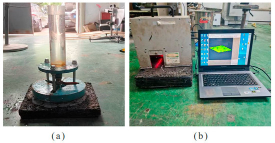
Figure 1.
(a) Schematic diagram of asphalt pavement permeability meter; (b) LS-40 acquisition device.
In Equation (1), Cw0 refers to the initial permeability coefficient of the PAM specimen (mL/min). V2 − V1 refers to the difference in water volume between the second and first readings (mL), and t2 − t1 refers to the time difference between the second and first readings(s).
2.3. Surface Texture Data Collection for Permeable Asphalt Pavements
In recent years, many researchers have investigated three-dimensional (3D) texture images and applied them in various fields. Hu et al. [31] employed eight different parameters to describe the 3D characteristics of macroscopic texture images based on 3D road surface data and qualitatively analyzed the influence of each parameter on macroscopic texture-related skid resistance. Li et al. [32] developed indicators to characterize the 3D features of both macroscopic road surface textures and microscopic aggregate textures, and established a road friction performance prediction model based on these surface and aggregate texture characteristics. Deng et al. [33] performed multi-scale power spectrum analysis of 3D pavement surface textures to predict the friction performance of asphalt pavement. Gao et al. [34] used CT scanning to analyze the internal structure of PAC and concluded that texture depth increases with porosity.
The 3D texture image features of permeable pavement effectively reflect clogging conditions and, in turn, indicate the permeability performance status of the pavement. Utilizing deep learning in combination with computer vision technology to analyze pavement images offers a theoretical foundation for the intelligent evaluation of the permeability performance levels of permeable pavements, and its procedure described in the following paragraph.
After recording the initial permeability coefficient of the PAM specimen, allow the specimen to dry for 24 h. Use a LS-40 portable ultra-high-resolution 3D laser imaging scanner to scan the surface of the PAM specimen, and after each blockage operation, wait until the surface of the PAM specimen is dry before using the LS-40. This is to avoid water light affecting the accurate data acquisition of the laser. Once the surface is dry, scan the PAM specimen using the LS-40 portable ultra-high-resolution 3D laser imaging scanner. Following each clogging operation, ensure the specimen’s surface is completely dry prior to scanning to avoid the interference of moisture and light on accurate laser data acquisition. The LS-40 can scan high-precision texture data within a range of 102 mm × 112 mm, capturing 2048 × 2048 data points. The horizontal precision is 0.05 mm, and the vertical precision is 0.01 mm. The 3D texture images of the PAM specimen are then collected. The specific image of collecting 3D texture images is shown in Figure 1b.
The 3D texture features of permeable pavements can reflect the clogging condition of the pavement, thereby judging the permeable performance state of permeable pavement. Using deep learning and computer vision techniques, pavement images can be analyzed to provide an intelligent evaluation of the permeability performance grade of permeable pavements.
2.4. Clogging Mechanism and Clogging Particle Testing Methods
The distribution and size of clogging particles significantly affect the water permeability performance of permeable pavements. However, particles that are either too coarse or too fine tend to have limited impact on clogging the pavement surface. Most studies have found that clogging primarily occurs in the surface or upper layers. Kayhanian et al. [35], through CT scan image analysis and core porosity distribution studies, observed that blockages generally form at or near the pavement surface. The American Concrete Institute (ACI) [36] noted that clogging is most likely when the particle size of the debris closely matches the void size in the pavement. Shan et al. [37] found that larger particles between 0.3 and 2.36 mm can significantly reduce permeability. Fwa et al. [38], in a comparative study of porous asphalt mixtures with different gradations, found that finer gradations were more susceptible to clogging. William et al. [34] demonstrated a strong correlation between aggregate gradation and permeability before and after clogging by evaluating ten commonly used porous asphalt gradations in the United States. Omkar et al. [39] showed that PAC with internal void diameters greater than 5–6 mm or less than 1–2 mm is less sensitive to clogging. Vancura [40] found that clogging particles rarely migrate deeper than 12.7 mm from the pavement surface. Kia et al. [41] reported that clogging initiates when sand and flocculent clay begin to accumulate near the upper surface of the specimen.
Since this is an indoor experiment requiring various permeability coefficients, the samples were manually clogged. After comprehensive consideration, fine aggregates with a particle size range of 0.075–4.75 mm were selected as the blocking material, with the gradation shown in Table 3.
Table 3.
Composition Table of Blockage Grading.
It is worth noting that the clogging simulation in this study is idealized to some extent. Environmental factors such as temperature and humidity fluctuations, as well as traffic-induced abrasion, were not considered. Moreover, real-world pavement clogging is a long-term and gradual process influenced by various interacting factors, including vehicle loads, water flow migration, and climatic conditions. In contrast, our experiment adopted a one-time, concentrated application of clogging materials under controlled conditions to ensure experimental consistency. This approach does not account for field mechanisms such as particle migration, compaction, or erosion, and therefore cannot fully represent the complex and dynamic nature of clogging evolution in actual pavement environments. As such, the results of the laboratory simulation are intended primarily to reveal the general trends in the relationship between clogging and permeability performance.
The experimental design is as follows:
- (1)
- The blocking materials listed in Table 3 are evenly spread across the surface of the PAM specimen in three stages. After lightly brushing the surface, 1000 mL of water is evenly applied to simulate the effect of rainfall, causing the blocking materials to clog the permeable asphalt pavement.
- (2)
- The PAM specimen treated in step (1) is left to dry for 24 h.
- (3)
- After collecting the texture data, the permeability coefficient is measured again using clean water.
- (4)
- Steps (1) to (3) are repeated until the permeability coefficient of the PAM specimen approaches 1200 mL/min, at which point the indoor clogging test is terminated.
3. Data Preprocessing and Augmentation
3.1. Data Preprocessing Stage
After data collection, both the 3D texture data files and the permeability coefficient data need to be preprocessed.
During the collection of the 3D texture data, fine dust particles in the air and the oily surface of the PAM specimen caused significant noise in the data captured by the LS-40 scanner. This noise included large outliers and impulse noise. Therefore, removing outliers from the 3D texture image data is a critical step in the preprocessing process.
3.1.1. Outlier Denoising
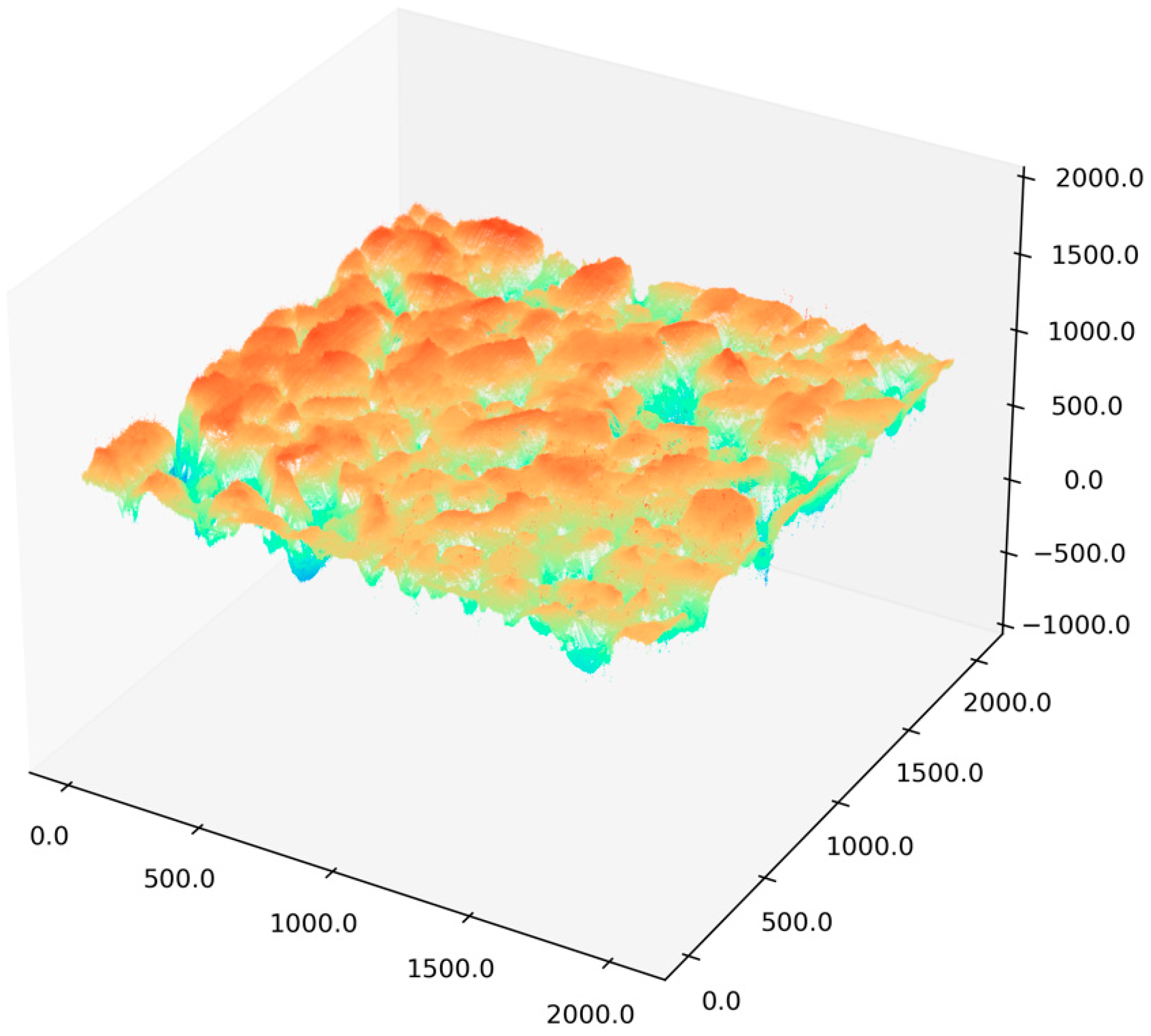
From Figure 2, it can be seen that there are significantly large outliers in the collected raw texture data, and there is a large deviation from the original data, with all such outliers exceeding a value of 2000. Therefore, a threshold of 2000 was set for threshold filtering, and noise points exceeding the threshold were replaced with the original data mean to effectively eliminate outliers.

Figure 2.
Three-dimensional reconstruction model.
3.1.2. Texture Surface Denoising
Common denoising methods include Gaussian filtering and median filtering. In this study, the MAD (Median Absolute Deviation) method was initially applied to remove small outliers from the texture data. The MAD-based outlier detection criteria are given by Equations (2) and (3).
Among them, xi is any data point in the 2048 × 2048 data matrix, median(x) is the median of the vector x, which consists of all data points, x is the data vector within a specified window size, and n is a parameter set to 3.
Fast Fourier Transform (FFT) was used to separate the image into macro-texture H0 and micro-texture W0. Then, wavelet denoising was applied to the micro-texture W0. This technique utilizes the multi-resolution analysis capability of wavelet transforms, applying thresholding to the wavelet coefficients to remove noise, resulting in the denoised micro-texture W1. Gaussian filtering was applied to the macro-texture H0 to smooth the image, producing the denoised macro-texture H1. The denoised macro-texture H1 and micro-texture W1 were then combined to reconstruct the preliminary texture signal Z1, as shown in the reconstruction formula:
Z1 = H1 + W1
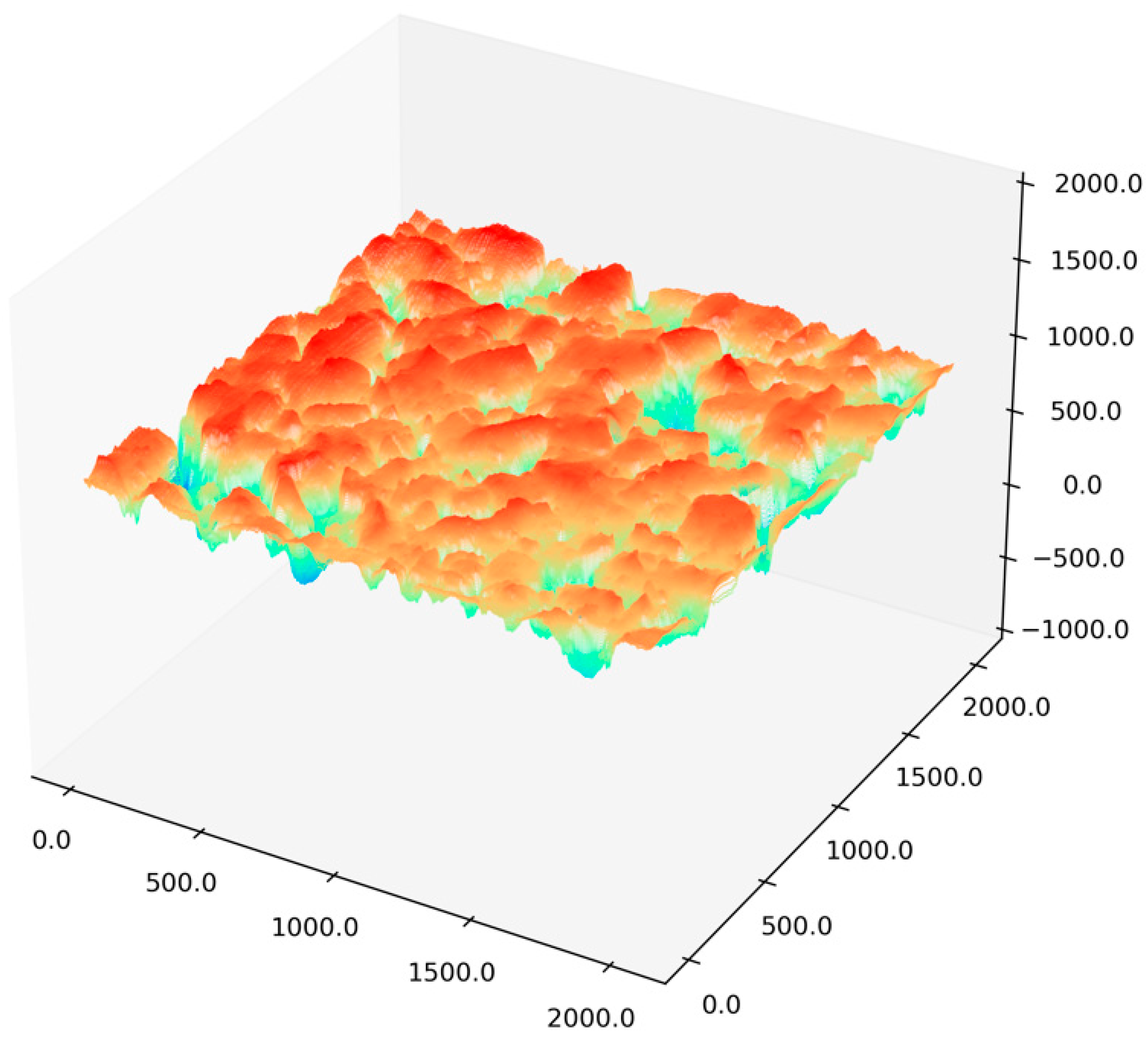
Finally, a Gaussian blur was applied to Z1 to obtain the final texture signal Z. The denoised image is shown in Figure 3. The methods used to obtain the denoised macro-texture H1 and the denoised texture signal Z are presented in Equations (5) and (6).

Figure 3.
Denoised 3D reconstruction.
The Gaussian kernel used for denoising, represented as Gaussian (x,y), where x and y are the horizontal and vertical distances from the center, has a standard deviation σ set to 1. This is a reasonable value as it preserves the image’s details and edge information better without excessive blurring.
3.1.3. Classification of Permeability Coefficient Labels
When processing the permeability coefficient data, the measured permeability coefficient is compared with the initial permeability coefficient, referred to as the permeability coefficient residual rate (γ). The calculation is given by Equation (7). Based on the value of γ, the permeability coefficient is classified into three categories: light blockage (Class A), moderate blockage (Class B), and severe blockage (Class C). Specifically, γ ≥ 90% corresponds to light blockage (Class A), 70% ≤ γ < 90% corresponds to moderate blockage (Class B), and γ ≤ 70% corresponds to severe blockage (Class C).
This classification scheme is flexible and can be adjusted according to different engineering requirements or regional standards. In this study, the thresholds of 90% and 70% were selected not only for their practical rationality in reflecting typical permeability degradation levels, but also to intentionally assess the model’s ability to distinguish cases with relatively small differences in permeability performance, particularly within the 70–90% range.
Among them, represents the current permeability coefficient, and represents the initial permeability coefficient.
3.2. Enhancement of Texture Image Data
The data used in this study consist entirely of three-dimensional texture data collected from indoor test specimens. Due to the limited quantity and low robustness of the original texture data, they are insufficient for training a neural network model. Therefore, it is necessary to enhance the original texture dataset.
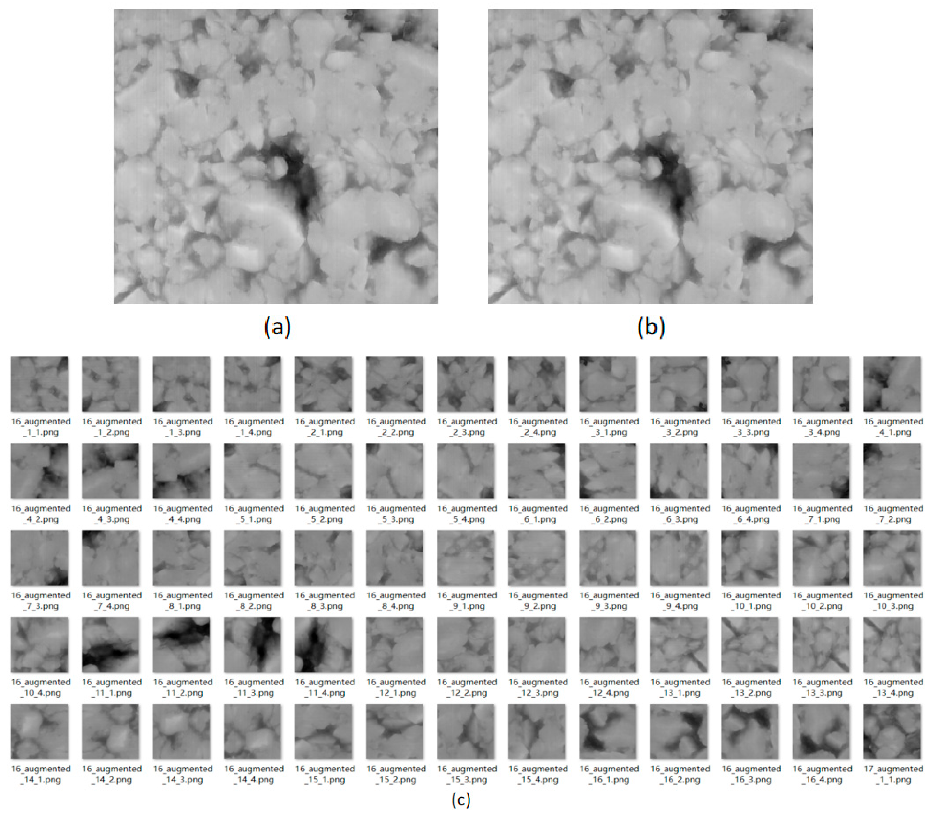
In the collected raw dataset, there are 20 data points for each of the three levels of mild blockage (Class A), moderate blockage (Class B), and severe blockage (Class C). First, the original dataset undergoes grayscale transformation, converting the data into 2048 × 2048 grayscale images, with 20 images per category. These grayscale images are then subjected to augmentation through rotation, flipping, and the addition of Gaussian noise, resulting in 256 images per category after processing. Although the neural network model requires input images sized at 224 × 224, this resolution was found to contain insufficient texture features to effectively support model training. Therefore, each image was seamlessly cropped to 512 × 512, and the model input size was adjusted accordingly. The cropping process is illustrated in Figure 4.
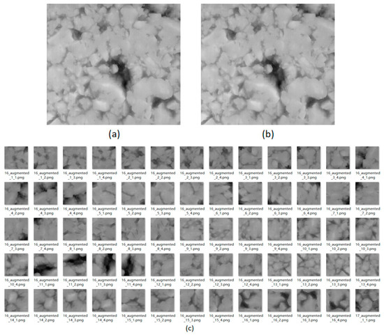
Figure 4.
(a) Original image; (b) grayscale image; (c) cropped image (data augmentation).
As seen in the figure, the cropped images contain different features. After data augmentation, there were 1034 images for each of the three categories, resulting in a total of 3072 images in the dataset. These were split into a training set and a validation set in a 0.7:0.3 ratio.
4. Experiment and Analysis
4.1. Residual Network
With the advancement of deep learning, intelligent analysis of road conditions using convolutional neural networks has become a prominent research area. Convolutional neural networks possess powerful feature extraction capabilities, leading to significant progress in road crack detection, road classification, and friction coefficient estimation. Nolte et al. [42] proposed a pavement condition classification method based on CNNs, which can be used to predict the friction coefficient. Dewangn et al. [43] developed an RCNet, a CNN-based road classification network, capable of accurately classifying five common types of pavements.
In addition to road surface monitoring, recent studies have demonstrated the broader applicability of machine learning and vision-based approaches in material and pavement performance evaluation. For instance, Xu et al. [44] measured the macroscopic texture index and reflectance coefficient of indoor rutting specimens and on-site asphalt pavement, and determined their correlation. On this basis, a multi-layer perceptron model based on the BP algorithm is used to construct a nonlinear model of the influence of macro- and micro-texture parameters on the retroreflection coefficient of asphalt pavement. Yu et al. [45], for effective characterization of asphalt surface texture characteristics, based on the principle of binocular stereo vision technology, developed a binocular camera texture detection system; the model of weak characteristic images of the same kind of pavement texture has a good recognition performance, and can effectively characterize asphalt pavement texture. Wang et al. [46] proposed the PT-SRGAN super-resolution network to enhance pavement texture measurements, enabling accurate reconstruction of 0.1 mm resolution 3D road surface textures from low-resolution laser data collected at higher speeds, thus improving the efficiency and flexibility of road texture evaluation. These studies, although targeting different materials or objectives, further validate the effectiveness of intelligent, data-driven approaches for infrastructure assessment.
This study utilizes a residual network as the training model for the collected dataset. During training, the residual neural network extracts features from the sample images, and the optimal network parameters are obtained through iterative validation, as detailed in Table 4. The specific structure of the model is shown in Table 5 and Figure 5.
Table 4.
Training Parameters.
Table 5.
Residual Network Structure.
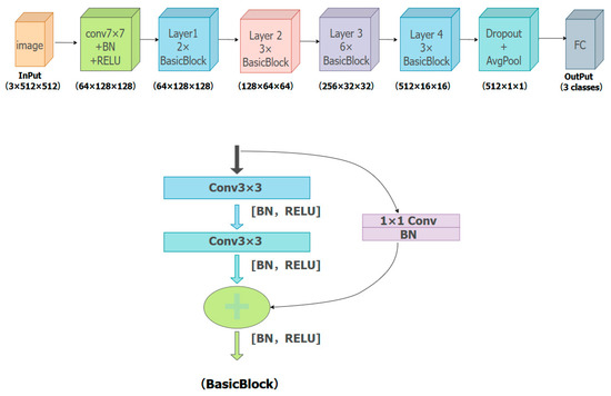
Figure 5.
Residual network model.
4.2. Evaluation
During training, F1-score and accuracy were used as evaluation metrics. The F1-score is a comprehensive metric introduced to balance the effects of accuracy and recall. It is particularly suitable for imbalanced classes and accounts for both precision and recall, preventing the model from overly favoring one of these measures. The F1-score is an effective metric for evaluating the overall performance of a classification model. The formula for calculating the F1-score is as follows:
4.3. Training Results and Analysis
Recent advances have demonstrated the growing role of machine learning and computer vision techniques in material and pavement performance evaluation. For instance, Xu et al. [46] evaluated the laboratory performance of composite materials using a waste-based approach without asphalt, applying vision-based assessments. Zhang et al. [45] predicted the compressive and flexural strength of a coal gangue-based geopolymer using machine learning models. Li et al. [46] constructed and optimized an asphalt pavement texture characterization model based on binocular vision and deep learning. Although these studies differ in material types or specific goals, they collectively reflect a trend toward intelligent, data-driven evaluation methods, which aligns with the objective of our research. These references support the feasibility and relevance of using deep learning models in assessing the permeability performance of porous asphalt pavements.
The weight update method adopted for model training is the Adam optimizer, which combines backpropagation and gradient descent to achieve the update. A learning rate scheduler was implemented, where the learning rate is halved (multiplied by 0.5) if the model’s performance on the validation set does not improve within 3 epochs. This approach helps avoid oscillations during steady periods or at local optima. The minimum learning rate was set to 1 × 10⁻⁶, and the optimal training parameters were obtained through repeated parameter tuning. To improve generalization and prevent overfitting, a dropout with a rate of 0.1 was introduced after the final residual block group (Layer4). This randomly disables a fraction of the neurons during training, forcing the network to learn more robust and distributed representations. In addition, L2 regularization was applied to the fully connected layer to penalize overly large weights, and batch normalization was incorporated after each convolution to stabilize and accelerate training.
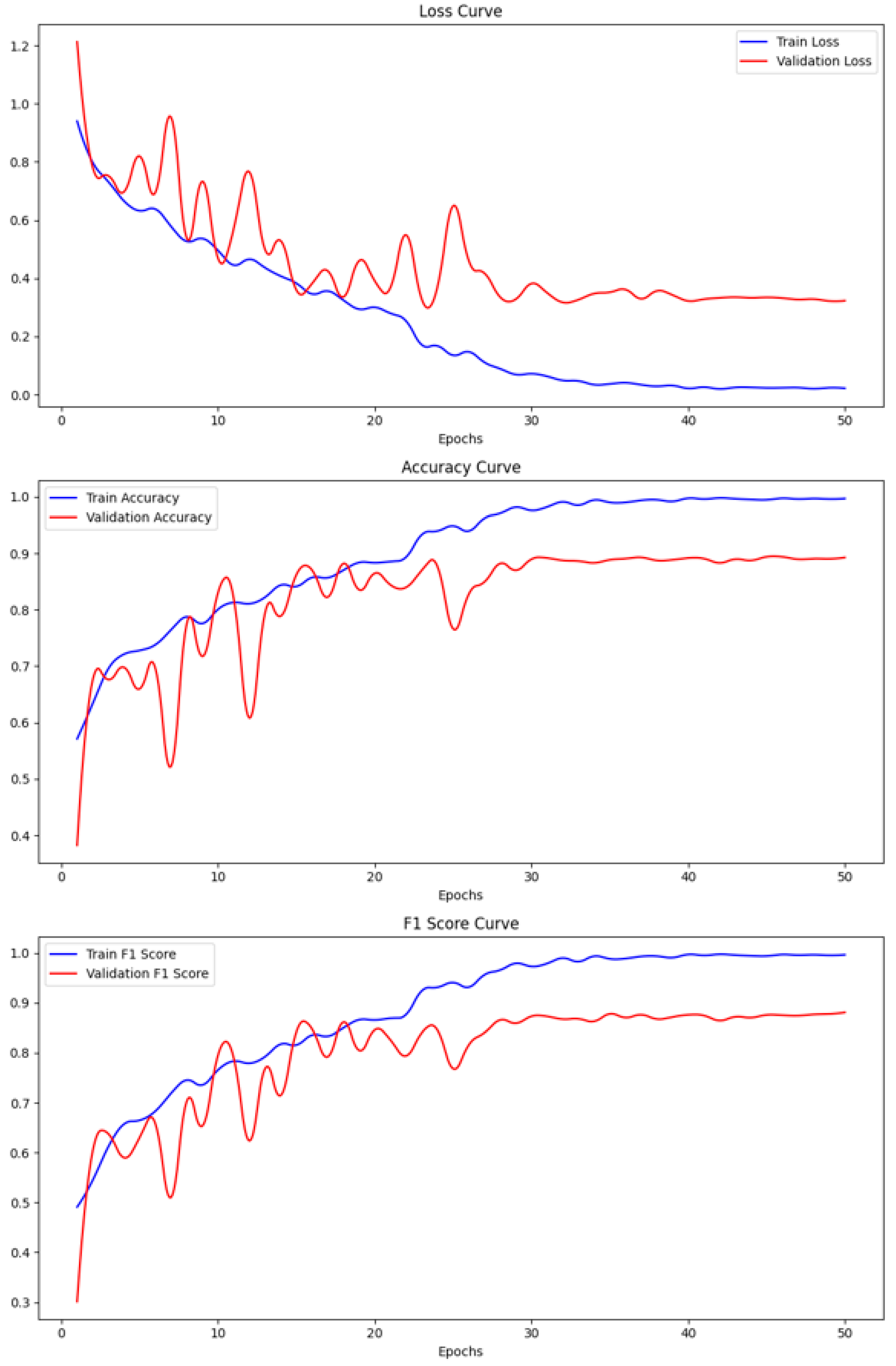
From the validation curve shown in Figure 6, it can be seen that as the number of iterations increases, the training accuracy, validation accuracy, and F1-score steadily improve without overfitting. Both training and validation losses decrease over time. Although some fluctuations were observed, the overall trend was upward. These results demonstrate the model’s effectiveness in evaluating the permeability function of permeable asphalt pavements. The model is capable of assessing permeability through 3D laser-imaged asphalt pavement images. Although minor fluctuations occur, the overall trend remains positive.
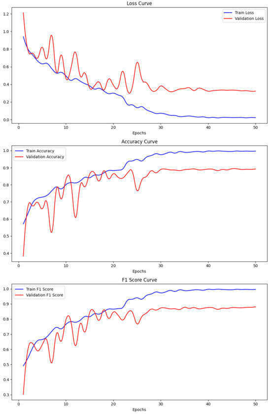
Figure 6.
Loss curve, Accuracy curve, and F1-score curve.
Table 6 compares the performance of different neural network architectures. In terms of accuracy, ResNet34 achieves the highest training accuracy at 98.88% and a validation accuracy of 90.32%. Inception V3 ranks second with 98.01% training accuracy and 89.79% validation accuracy. VGG16 follows with 94.37% and 88.49%, respectively, while ResNet18 performs the lowest at 92.52% and 86.38%.
Table 6.
Compare the results with other models.
Regarding F1-score, all four models exceed 85%. ResNet34 ranks first again, achieving 98.68% on the training set and 89.66% on the validation set. Inception V3 follows with 96.79% and 89.25%. ResNet18 ranks third at 94.21% and 85.69%, while VGG16 is fourth with 92.47% and 86.25%.
These results indicate that ResNet34 is the model with the best performance among several models. This model can evaluate the permeability and blockage of road surfaces through three-dimensional laser imaging of permeable asphalt pavement images.
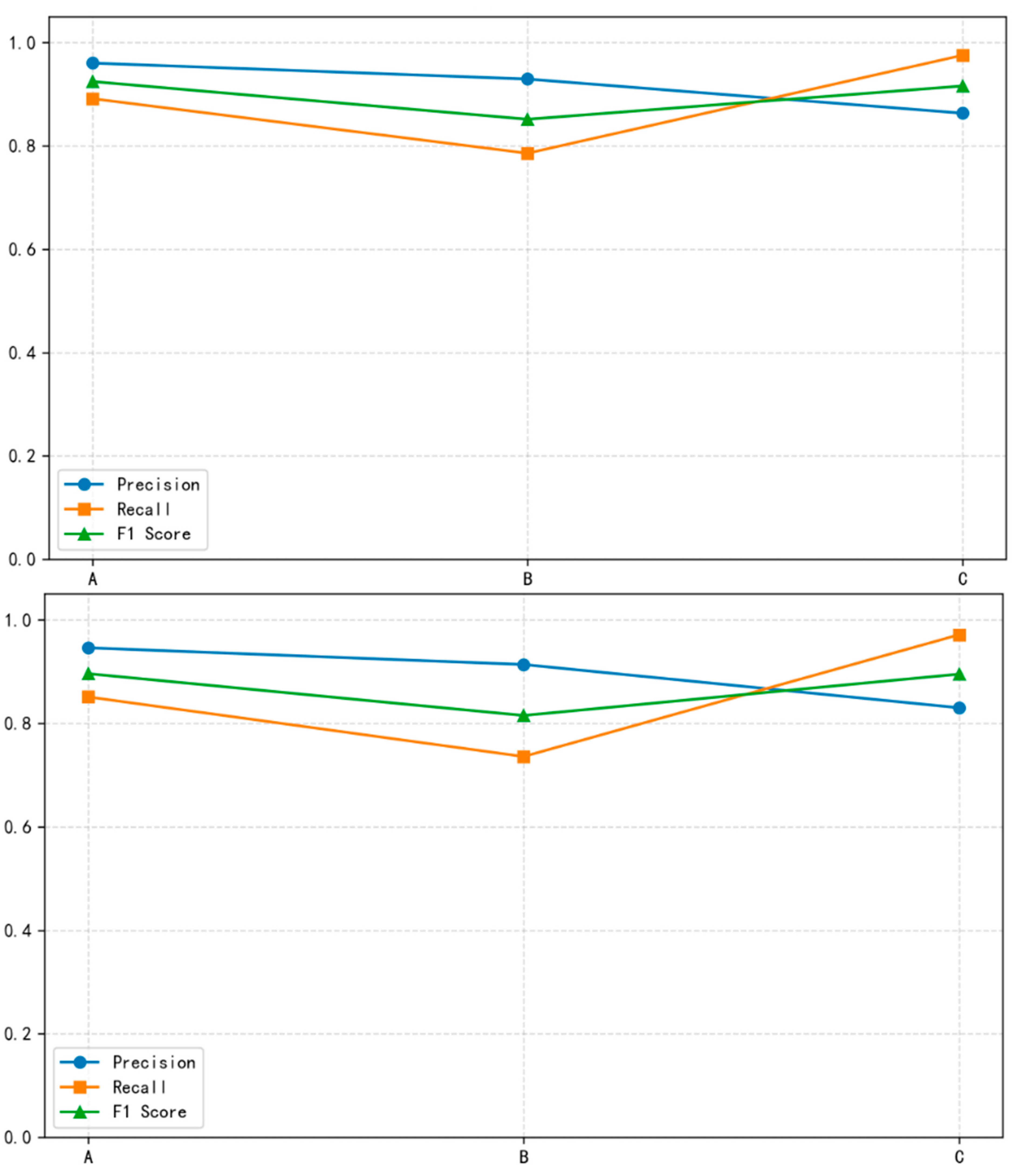
To further evaluate the performance of the proposed model, a baseline comparison was conducted using support vector machine (SVM) regression. The SVM was trained on the same dataset with identical input features. As shown in Table 7 and Figure 7, the neural network significantly outperformed the SVM in both training and validation accuracy. This confirms that deep learning methods offer superior capability in capturing complex texture features of 3D pavement surfaces compared to traditional regression models.
Table 7.
SVM algorithm results.
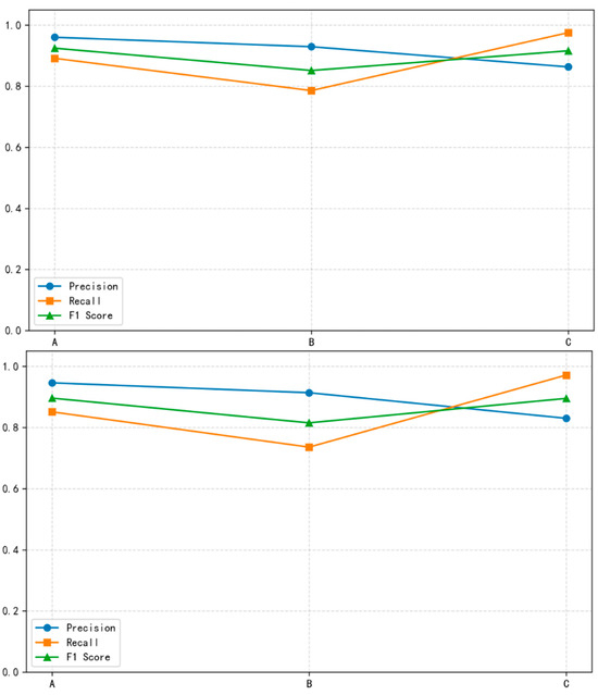
Figure 7.
SVM training set (the first) and validation set rendering (the second).
5. Conclusions
- (1)
- In this study, three-dimensional laser scanning and image processing techniques were employed to acquire and refine the 3D texture data of porous asphalt concrete (PAC), which contained substantial noise. By separating macro- and micro-level texture information, outlier removal and Fourier transform-based methods were used for targeted denoising. Different approaches were applied to macro- and micro-textures, respectively, to preserve the local surface features, ensuring the integrity and reliability of the processed image data.
- (2)
- The applicability of different test methods was analyzed through permeability experiments. In combination with previous research, the study explored key influencing factors and clogging mechanisms that affect the water permeability performance of PAC-13. Results indicate that, beyond void ratio, aggregate gradation, and particle characteristics, the type and distribution of blockages also play a critical role. Moreover, the proper selection of maintenance and cleaning strategies is essential for preserving long-term permeability performance. These findings offer a scientific basis for the design, construction, and maintenance of porous asphalt concrete, enhancing road safety and extending service life. Future studies may focus on the adaptability of the intelligent evaluation model under varying road conditions and integrate multi-source data to further improve prediction accuracy. Additionally, optimization of clog removal methods could further strengthen the anti-clogging capacity and durability of drainage pavements.
- (3)
- This research integrates traditional convolutional neural networks with advanced deep learning techniques to develop an innovative intelligent evaluation model based on 3D laser imaging for assessing the surface permeability functionality of porous asphalt pavements. The model, characterized by its non-destructive and high-efficiency nature, can rapidly and accurately predict the seepage performance of permeable asphalt pavement and evaluate the surface condition of porous asphalt pavements. The validation set achieved an accuracy of 90.36% and an F1-score of 90.33%. Through extensive training, the model demonstrated enhanced robustness and can output high-reliability, repeatable, and quickly acquired network-level data. These outputs serve as a robust foundation for maintenance decision-making in expressway drainage systems, including determining optimal maintenance timing, selecting appropriate methods, and identifying precise maintenance targets—thus providing strong technical support for the development of “smart expressways”.
Author Contributions
Conceptualization, Y.Z. and J.L.; methodology, Y.Z. and X.L.; software, J.L., R.X. and Y.Z.; validation, J.L. and Y.Z.; formal analysis, R.X., R.C. and W.L.; investigation, J.L., Y.Z. and R.X.; resources, R.X.; data curation, J.L. and X.L.; writing—original draft preparation, J.L. and R.X.; writing—review and editing, Y.Z.; visualization, W.L.; supervision, J.L., R.C. and Y.Z.; project administration, J.L.; funding acquisition, R.X. and Y.Z. All authors have read and agreed to the published version of the manuscript.
Funding
This research was funded by the National Natural Science Foundation of China: Time-varying Coupling contact Behavior characteristics of Tires and Roads in Alpine Regions and Intelligent Prediction of Pavement Anti-skid Performance Decay [grant number 52478471], the Chongqing Technology Innovation and Application Development Project: Sichuan–Chongqing Science and Technology Innovation Cooperation Program, [grant number CSTB2024TIAD-CYKJCXX0004], and the Sichuan Transportation Construction Group Co., Ltd. Technology Project, [Project Number 2023-CMLM-46].
Data Availability Statement
Due to the nature of this research, participants of this study did not agree for their data to be shared publicly, so supporting data are not available.
Conflicts of Interest
Authors Rui Xiao, Xin Li, Rong Chen and Wenjie Li were employed by Sichuan Provincial Transportation Construction Group Co., Ltd. The remaining authors declare that the research was conducted in the absence of any commercial or financial relationships that could be construed as a potential conflict of interest.
References
- Qiao, X.J.; Liao, K.H.; Randrup, T.B. Sustainable stormwater management: A qualitative case study of the Sponge Cities initiative in China. Sustain. Cities Soc. 2019, 53, 101963. [Google Scholar] [CrossRef]
- Guo, X.; Zhang, J.; Zhou, B.; Liu, W.; Pei, J.; Guan, Y. Sponge roads: The permeable asphalt pavement structures based on rainfall characteristics in central plains urban agglomeration of China. Water Sci. Technol. 2019, 80, 1740–1750. [Google Scholar] [CrossRef] [PubMed]
- Pratt, C.J.; Mantle, J.D.G.; Schofield, P.A. UK research into the performance of permeable pavement, reservoir structures in controlling stormwater discharge quantity and quality. Water Sci. Technol. 1995, 32, 63–69. [Google Scholar] [CrossRef]
- Hu, J.; Ma, T.; Ma, K. DEM-CFD simulation on clogging and degradation of air voids in double-layer porous asphalt pavement under rainfall. J. Hydrol. 2021, 595, 126028. [Google Scholar] [CrossRef]
- Alvarez, A.E.; Martin, A.E.; Estakhri, C. Drainability of permeable friction course mixtures. J. Mater. Civ. Eng. 2010, 22, 556–564. [Google Scholar] [CrossRef]
- Alvarez, A.E.; Martin, A.E.; Estakhri, C. A review of mix design and evaluation research for permeable friction course mixtures. Constr. Build. Mater. 2011, 25, 1159–1166. [Google Scholar] [CrossRef]
- Zhang, Y.; Ven, M.V.D.; Molenaar, A.; Wu, S. Preventive maintenance of porous asphalt concrete using surface treatment technology. Mater. Des. 2016, 99, 262–272. [Google Scholar] [CrossRef]
- Takahashi, S. Comprehensive study on the porous asphalt effects on expressways in Japan: Based on field data analysis in the last decade. Road Mater. Pavement Des. 2013, 14, 239–255. [Google Scholar] [CrossRef]
- Zhan, Y.; Li, Q.J.; Yang, G.; Wang, K.C. Performance monitoring of pavement surface characteristics with 3D surface data. Airfield Highw. Pavements 2017, 2017, 195. [Google Scholar] [CrossRef]
- Li, Q.; Yang, G.; Wang, K.C.P.; Zhan, Y.; Wang, C. Novel macro-and microtexture indicators for pavement friction by using high-resolution three-dimensional surface data. Transp. Res. Rec. 2017, 2641, 164–176. [Google Scholar] [CrossRef]
- Zhou, X.-L.; Jiang, N.-D.; Xiao, W.-X.; Ran, M.-P.; Xie, X.-F. Measurement Method for Mean Texture Depth of Asphalt Pavement Based on Laser Vision. China J. Highw. Transp. 2014, 27, 11–16. [Google Scholar] [CrossRef]
- Dou, G.W. Research of calculation model of pavement texture depth based on profile elevation. J. Highw. Transp. Res. Dev. 2015, 32, 7. [Google Scholar] [CrossRef]
- Cigada, A.; Mancosu, F.; Manzoni, S.; Zappa, E. Laser-triangulation device for in-line measurement of road texture at medium and high speed. Mech. Syst. Signal Process. 2010, 24, 2225–2234. [Google Scholar] [CrossRef]
- Yang, G.; Li, Q.J.; Zhan, Y.; Fei, Y.; Zhang, A. Convolutional neural network–based friction model using pavement texture data. J. Comput. Civ. Eng. 2018, 32, 04018052. [Google Scholar] [CrossRef]
- Alamdarlo, M.N.; Hesami, S. Optimization of the photometric stereo method for measuring pavement texture properties. Measurement 2018, 127, 406–413. [Google Scholar] [CrossRef]
- Ouyang, W.; Xu, B. Pavement cracking measurements using 3D laser-scan images. Meas. Sci. Technol. 2013, 24, 105204. [Google Scholar] [CrossRef]
- Wang, Z.; Xie, J.; Gao, L.; Liu, Y.; Tang, L. Three-dimensional characterization of air voids in porous asphalt concrete. Constr. Build. Mater. 2021, 272, 121633. [Google Scholar] [CrossRef]
- Zhan, Y.; Li, J.Q.; Yang, G.; Wang, K.C.P.; Yu, W. Friction-ResNets: Deep residual network architecture for pavement skid resistance evaluation. J. Transp. Eng. Part B Pavements 2020, 146, 04020027. [Google Scholar] [CrossRef]
- Kandhal, P.S.; Mallick, R.B. Effect of mix gradation on rutting potential of dense-graded asphalt mixtures. Transp. Res. Rec. 2001, 1767, 146–151. [Google Scholar] [CrossRef]
- Shi, S.; Jiang, L.; Deng, J.; Wang, Z.; Guo, C.; Shi, J.; Wang, X.; Li, H. PV-RCNN++: Point-voxelfeature set abstraction with local vector representation for 3d objectdetection. Int. J. Comput. Vis. 2023, 131, 531–551. [Google Scholar] [CrossRef]
- Chen, H.; Zhang, D.; Gui, R.; Pu, F.; Cao, M.; Xu, X. 3D pavement data decomposition and texture levelevaluation based on step extraction and Pavement-Transformer. Measurement 2022, 188, 110399. [Google Scholar] [CrossRef]
- Dong, S.; Han, S.; Wu, C.; Xu, O.; Kong, H. Asphalt pavement macrotexture reconstruction frommonocular image based on deep convolutional neural network. Comput.-Aided Civiland Infrastruct. Eng. 2022, 37, 1754–1768. [Google Scholar] [CrossRef]
- Maupin, G.W., Jr. Asphalt permeability testing: Specimen preparation and testing variability. Transp. Res. Rec. 2001, 1767, 33–39. [Google Scholar] [CrossRef]
- Kanitpong, K.; Benson, C.H.; Bahia, H.U. Measuring and predicting hydraulic conductivity (permeability) of compacted asphalt mixtures in the 1aboratory. In Proceedings of the 82nd Annual Meeting of the Transportation Research Board, Washington, DC, USA, 12–16 January 2003. [Google Scholar] [CrossRef]
- Kuang, X.; Kim, J.-Y.; Gnecco, I.; Raje, S.; Garofalo, G.; Sansalone, J.J. Particle separation and hydrologic control by permeable pavement. Transp. Res. Rec. 2007, 2025, 111–117. [Google Scholar] [CrossRef]
- Fwa, T.F.; Ong, G.P. Wet pavement hydroplaning risk and skid resistance: Analysis. J. Transp. Eng. 2008, 134, 182–190. [Google Scholar] [CrossRef]
- Adhara, C.T. Probabilistic analysis of air void structure and its relationship to permeability and moisture damage of hot mix asphalt. Ph.D. Thesis, Texas A&M University, College Station, TX, USA, 2004. Available online: http://hdl.handle.net/1969.1/3114 (accessed on 3 April 2025).
- Montes, F.; Haselbach, L. Measuring hydraulic conductivity in pervious concrete. Environ. Eng. Sci. 2006, 23, 960–969. [Google Scholar] [CrossRef]
- Li, Z.; Guo, T.; Chen, Y.; Zhang, M.; Xu, Q.; Wang, J.; Jin, L.; Diab, A. Study on properties of drainage SBS modified asphalt mixture with fiber. Adv. Civ. Eng. 2021, 2021, 7846499. [Google Scholar] [CrossRef]
- Martin, W.D.; Putman, B.J.; Neptune, A.I. Influence of aggregate gradation on clogging characteristics of porous asphalt mixtures. J. Mater. Civ. Eng. 2014, 26, 04014026. [Google Scholar] [CrossRef]
- Hu, L.; Yun, D.; Liu, Z.; Du, S.; Zhang, Z.; Bao, Y. Effect of three-dimensional macrotexture characteristics on dynamic frictional coef-ficient of asphalt pavement surface. Constr. Build. Mater. 2016, 126, 720–729. [Google Scholar] [CrossRef]
- Li, Q.J.; Zhan, Y.; Yang, G.; Wang, K.C.P. Pavement skid resistance as a function of pavement surface and aggregate texture properties. Int. J. Pavement Eng. 2020, 21, 1159–1169. [Google Scholar] [CrossRef]
- Deng, Q.; Zhan, Y.; Liu, C.; Qiu, Y.; Zhang, A. Multiscale power spectrum analysis of 3D surface texture for prediction of asphalt pavement friction. Constr. Build. Mater. 2021, 293, 123506. [Google Scholar] [CrossRef]
- Gao, L.; Liu, M.; Wang, Z.; Xie, J.; Jia, S. Correction of texture depth of porous asphalt pavement based on CT scanning technique. Constr. Build. Mater. 2019, 200, 514–520. [Google Scholar] [CrossRef]
- Kayhanian, M.; Anderson, D.; Harvey, J.T.; Jones, D.; Muhunthan, B. Permeability measurement and scan imaging to assess clogging of pervious concrete pavements in parking lots. J. Environ. Manag. 2012, 95, 114–123. [Google Scholar] [CrossRef]
- ACI. ACI 522R-10: Report on Pervious Concrete; ACI Committee 522: Farmington Hills, MI, USA, 2010. [Google Scholar]
- Shan, J.; Feng, S.; Li, F.; Wu, S. Lateral permeability of pervious asphalt mixtures and the influence of clogging. Constr. Build. Mater. 2021, 273, 121988. [Google Scholar] [CrossRef]
- Fwa, T.F.; Tan, S.A.; Guwe, Y.K. Laboratory Evaluation of Clogging Potential of Porous Asphalt Mixtures. Transp. Res. Rec. 1999, 1681, 43–49. [Google Scholar] [CrossRef]
- Deo, O.; Sumanasooriya, M.; Neithalath, N. Permeability reduction in pervious concretes due to clogging: Experiments and modeling. J. Mater. Civ. Eng. 2010, 22, 741–751. [Google Scholar] [CrossRef]
- Vancura, M.E.; MacDonald, K.; Khazanovich, L. Location and depth of pervious concrete clogging material before and after void maintenance with common municipal utility vehicles. J. Transp. Eng. 2012, 138, 332–338. [Google Scholar] [CrossRef]
- Kia, A.; Wong, H.S.; Cheeseman, C.R. Defining clogging potential for permeable concrete. J. Environ. Manag. 2018, 220, 44–53. [Google Scholar] [CrossRef]
- Nolte, M.; Kister, N.; Maurer, M. Assessment of deep convolutional neural networks for road surface classification. In Proceedings of the 21st International Conference on Intelligent Transportation Systems (ITSC), Maui, HI, USA, 4–7 November 2018; IEEE: Piscataway, NJ, USA, 2018; pp. 381–386. [Google Scholar] [CrossRef]
- RCDewangan, D.K.; Sahu, S.P. RCNet: Road classification convolutional neural networks for intelligent vehicle system. Intell. Serv. Robot. 2021, 14, 199–214. [Google Scholar] [CrossRef]
- Xu, P.; Qian, G.; Zhang, C.; Wang, X.; Yu, H.; Zhou, H.; Zhao, C. Influence of the Surface Texture Parameters of Asphalt Pavement on Light Reflection Characteristics. Appl. Sci. 2023, 13, 12824. [Google Scholar] [CrossRef]
- Yu, M.; Zhang, R.; Tang, O.; Jin, D.; You, Z.; Zhang, Z. Construction and optimization of asphalt pavement texture characterization model based on binocular vision and deep learning. Measurement 2025, 248, 116946. [Google Scholar] [CrossRef]
- Wang, G.; Wang, K.C.P.; Yang, G. Deep learning based image reconstruction at any speeds for faster pavement texture measurement using 3D laser technology. Int. J. Pavement Eng. 2023, 24, 2269461. [Google Scholar] [CrossRef]


Disclaimer/Publisher’s Note: The statements, opinions and data contained in all publications are solely those of the individual author(s) and contributor(s) and not of MDPI and/or the editor(s). MDPI and/or the editor(s) disclaim responsibility for any injury to people or property resulting from any ideas, methods, instructions or products referred to in the content. |
© 2025 by the authors. Licensee MDPI, Basel, Switzerland. This article is an open access article distributed under the terms and conditions of the Creative Commons Attribution (CC BY) license (https://creativecommons.org/licenses/by/4.0/).