Article

Monitoring and Prediction of the Real-Time Transient Thermal Mechanical Behaviors of a Motorized Spindle Tool

1
Mechanical Engineering Department, Politeknik Negeri Bandung, Bandung 40559, Indonesia
2
Graduate Institute of Precision Manufacturing, National Chin-Yi University of Technology, Taichung 411030, Taiwan
3
Department of Mechanical Engineering, National Chin-Yi University of Technology, Taichung 411030, Taiwan
4
Department of Manufacturing Design Engineering, Politeknik Manufaktur Bandung, Bandung 40135, Indonesia
*
Author to whom correspondence should be addressed.
Lubricants 2025, 13(6), 269; https://doi.org/10.3390/lubricants13060269
Submission received: 27 May 2025 / Revised: 13 June 2025 / Accepted: 15 June 2025 / Published: 16 June 2025
(This article belongs to the Special Issue High Performance Machining and Surface Tribology)

Abstract

The spindle is a critical component that significantly influences the performance of machine tools. In motorized spindles, heat generation from both the bearings and built-in motor leads to thermal deformation of structural components, which, in turn, affects machining accuracy. This study investigates the thermo-mechanical behavior of motorized spindles under various operational conditions, with the aim of accurately predicting thermally induced axial deformation and determining optimal temperature sensor placement. To achieve this, temperature rise and deformation data were simultaneously collected using appropriate data acquisition systems across varying spindle speeds. A correlation analysis confirmed a strong positive relationship exceeding 97.5% between temperature rise at all sensor locations and axial thermal deformation. Multivariate regression analysis was then applied to identify optimal combinations of sensor data for accurate deformation prediction. Additionally, a finite element (FE) thermal–mechanical model was developed to simulate spindle behavior, with the results validated against experimental measurements and regression model predictions. The four-variable regression model and FE simulation achieved Root Mean Square Errors (RMSEs) of 0.84 µm and 0.82 µm, respectively, both demonstrating close agreement with experimental data and effectively capturing the trend of thermal deformation over time under different operating conditions. Finally, an optimal sensor configuration was identified that minimizes pre-diction error while reducing the number of required sensors. Overall, the proposed methodology offers valuable insights for optimizing spindle design to enhance thermal–mechanical performance.

1. Introduction

The motorized spindle is a critical component of modern machine tools in determining the overall accuracy and performance of machining operations. This makes the monitoring and prediction of its thermal behavior an essential task [1]. Before machining, high-precision machine tools typically require an extended preheating period to reach thermal equilibrium [2]. However, thermal deformation arising from complex heat transfer phenomena during precision machining remains a persistent obstacle to achieving high machining accuracy [3]. The ongoing demand for ultra-precision manufacturing highlights the necessity of a comprehensive understanding and effective control of thermal deformation in machine tools, particularly within the motorized spindle [4]. As one of the primary sources of error in CNC machining, thermal deformation is induced by internal heat sources, including those resulting from ambient temperature fluctuations, viscous friction, and cutting loads, all of which significantly affect positional and dimensional accuracy [5]. Additionally, changes in bearing preload influence spindle temperature, which, in turn, affects the dynamic behavior of the spindle system [6,7]. The rise in spindle temperature and the resulting thermal deformation compensation in machine tools have been subjects of academic research since the 1960s. Both academia and industry have made considerable progress in developing and applying thermal error compensation technologies [8,9], as well as in the modeling [10,11,12,13,14,15,16] and prediction [12,17,18,19,20] of thermal behavior in machine tools. In addition to effectively mitigating spindle temperature rise, spindle thermal displacement compensation has become a widely adopted method for controlling positioning errors caused by thermal deformation.
Recent developments in the field emphasize the integration of advanced sensor technologies, sophisticated modeling approaches, and machine learning algorithms to improve the accuracy and reliability of thermal deformation monitoring and prediction. Among these, fiber Bragg grating (FBG) sensors—known for their high sensitivity and resistance to electromagnetic interference—have become increasingly popular for real-time temperature monitoring at critical locations within the spindle system [21]. Advanced machine learning techniques are also being employed to predict thermal errors in motorized spindles with high precision [22]. For example, hybrid models combining regression analysis with fuzzy inference systems have been proposed to optimize thermal variables and effectively compensate for thermal displacement errors in CNC machine tools [23]. A convolutional neural network (CNN)-based method has demonstrated superior performance in estimating thermal displacement compared to traditional models [24]. Integrating multiple data sources, such as temperature and vibration signals, enhances the accuracy of thermal deformation predictions [25]. One study proposed a method that fuses heterogeneous information sources using support vector regression (SVR) to predict thermal deformation in spindle systems, achieving higher accuracy than temperature-based models alone [26]. Additionally, the digital twin (DT) paradigm, when combined with long short-term memory (LSTM) networks—referred to as the DT-LSTM approach—has been applied for real-time prediction of thermal errors in CNC spindle systems, yielding an approximate 11% improvement in accuracy compared to individual prediction methods [27,28,29].
In addition to the prediction of thermal deformation, real-time monitoring and compensation of thermal-induced deformation play a critical role in maintaining machining accuracy and optimizing the performance of motorized spindles. Accurate prediction of thermal deformation enables the implementation of proactive compensation strategies, thereby minimizing machining errors and ensuring the dimensional accuracy of finished components. Real-time compensation of geometric and thermal errors in machine tools can be implemented through external compensation systems that interface with NC controllers and multi-axis systems. Many studies have explored thermal error modeling and compensation using a variety of models and algorithms. For instance, Zhang et al. [20] proposed a comprehensive spindle thermal error compensation method that integrated a CNC interface compensation module with a thermal error prediction model, which was established on the basis of gated recurrent unit (GRU) with improved Monte Carlo cross-validation. The compensation system was successfully verified on a CNC grinding machine, achieving a residual displacement error of less than 3.4 μm after compensation. Lee and Yang [30] utilized a two-sphere probe to identify geometric and thermal error sources along the X-, Y-, and Z-axes. They developed a neural network-based mathematical model to predict thermal errors, demonstrating high reliability and stability in their predictions. Miao et al. [31,32] proposed combining multiple linear regression (MLR) with principal component regression (PCR) to mitigate the effects of multicollinearity among temperature variables in thermal error modeling. Wei et al. [14] proposed Gaussian process regression (GPR) as a thermal error modeling method, which can provide internal thermal error prediction, high accuracy, and robustness. Liu et al. [33] demonstrated that long short-term memory (LSTM) networks can capture the hysteresis effects inherent in thermal expansion. Yu et al. [34] applied multiple regression techniques to thermal error compensation in a workpiece spindle lathe, achieving forecasting errors within 5 µm. Maurya et al. [35] adopted an artificial neural network (ANN) approach for thermal error prediction, optimizing the model inputs by incorporating cooling channel parameters such as the supply coolant temperature, temperature difference between the spindle inlet and outlet, and coolant flow rate.
Thermo-structural coupling theories and finite element modeling (FEM) have also been extensively used to analyze thermal deformation in motorized spindles [36]. A study based on these theories developed and experimentally validated a model capable of predicting temperature distribution and structural deformation under varying operating conditions [18]. Furthermore, global sensitivity analysis using Kriging surrogate models has been employed to evaluate the reliability of thermal deformation predictions, revealing the significant impact of factors such as the spindle rotational speed and cooling conditions [27]. Several researchers have explored the use of numerous sensors initially and then reduced the number to an optimized subset to improve the accuracy and robustness of thermal error predictions. Tan et al. [37] selected three key temperature points out of twenty by utilizing the least-squares support vector machine (SVM) as the baseline thermal error model, combined with the bat binary algorithm for optimization. Liu et al. [38] started with ten temperature sensor positions and reduced them to the two most sensitive points, applying principal component regression (PCR) for modeling. This approach achieved Z-direction spindle error compensation within 10 µm. Similarly, Liu et al. [11] also used ten temperature sensors and implemented a temperature-sensitive point (TSP) selection method, identifying a stable two-sensor combination for optimal performance. Ariaga et al. [39] deployed 38 temperature sensors and selected 9 and 10 sensors using ANFIS and artificial neural network (ANN) methods, respectively. Cheng et al. [40] proposed a new method for accurately predicting thermal displacement in motorized spindles using a Bald Eagle Search (BES) algorithm–optimized least-squares support vector machine (LSSVM), in which the key temperature points were selected using K-means clustering and gray correlation analysis. This method was verified to model the nonlinear relationship between temperature and displacement. Cao et al. [41] proposed the GTF method to improve correlation and diversity in KTP selection for thermal error modeling in machine tools with multiple heat sources. This method, which combined the gray relational analysis, thermal sensitivity, and fuzzy c-means clustering, was successfully validated on a vertical machining center and a large floor-type boring machine, significantly reducing the prediction error and RMSE by about 28% and 25.8%. These studies clearly imply that although using a large number of sensors enhances the robustness of thermal error models, it increases system complexity and costs and reduces practicality for real-world applications. Effective thermal error compensation critically depends on real-time temperature data obtained from strategically positioned sensors that accurately capture the dynamic thermal behavior of the spindle system. Thus, optimizing sensor placement remains a key challenge in the development of reliable thermal deformation monitoring and prediction systems. Moreover, real-time monitoring and prediction of thermal deformation offer an effective means of optimizing motorized spindle performance by minimizing thermal effects under varying operational conditions.
This study aims to experimentally investigate the transient thermo-mechanical behavior of a motorized spindle and to establish the relationship between temperature rise measured at various sensor locations and the resulting thermal deformation. Some novelty and contribution are expected to come from this study, including (1) the development of a combined experimental and finite element (FE) thermal–mechanical modeling approach to analyze spindle deformation under varying operational conditions; (2) the demonstration of a strong correlation (>97.5%) between local temperature rise and axial thermal displacement; (3) the proposal of a regression-based method for optimal sensor placement, allowing for reliable deformation prediction with as few as one or two sensors; (4) the validation of a thermal–mechanical FE model that can be used as a digital surrogate for generating data and supporting real-time prediction; and (5) a cost-effective, scalable method that supports future integration into digital twin systems and real-time thermal compensation frameworks for high-precision machining. This paper is organized as follows: Section 2 describes the experimental setup for thermal data acquisition and spindle deformation measurement and presents the data analysis methodology, including correlation and multivariate regression analysis for sensor placement optimization. Section 3 details the thermal–mechanical finite element modeling and validation process. Section 4 discusses the results and implications, especially regarding industrial applicability. Section 5 concludes the paper and outlines directions for future research.

2. Experimental Approach

The overall methodology of this study comprises three main stages (see Figure 1):
  • Experimental measurement of spindle temperature rise and thermal displacement;
  • Data analysis, including correlation assessment and multivariate regression to evaluate potential sensor–placement combinations;
  • Prediction-model selection based on minimizing displacement error while using the fewest sensors.
Figure 1 presents a detailed architectural flowchart for the predictive modeling process. First, the experimental apparatus is configured to collect temperature and displacement data during spindle run-in tests. These data undergo iterative correlation analysis, refining sensor combinations until a Pearson correlation coefficient of 0.9 is achieved. In parallel, FEM is performed to simulate heat generation and convection using established empirical formulas; the FEM results are continuously compared with experimental measurements. Once the correlation threshold is reached, the workflow proceeds to regression analysis, model selection, and model verification. Finally, FEM is employed again to simulate the spindle’s thermo-mechanical behavior under varied operating conditions. The process culminates in a systematically validated predictive model—optimized for accuracy and sensor efficiency—which can be deployed for real-time monitoring and prediction of spindle thermal errors.

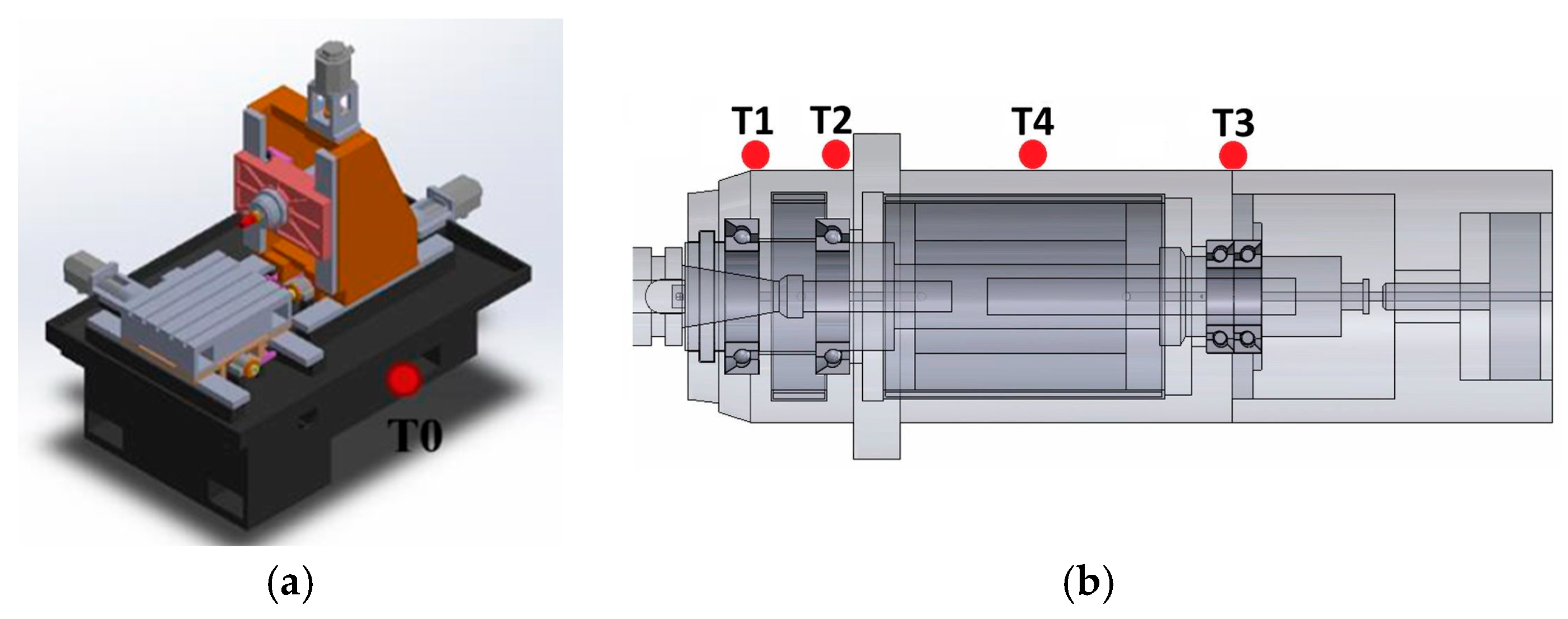
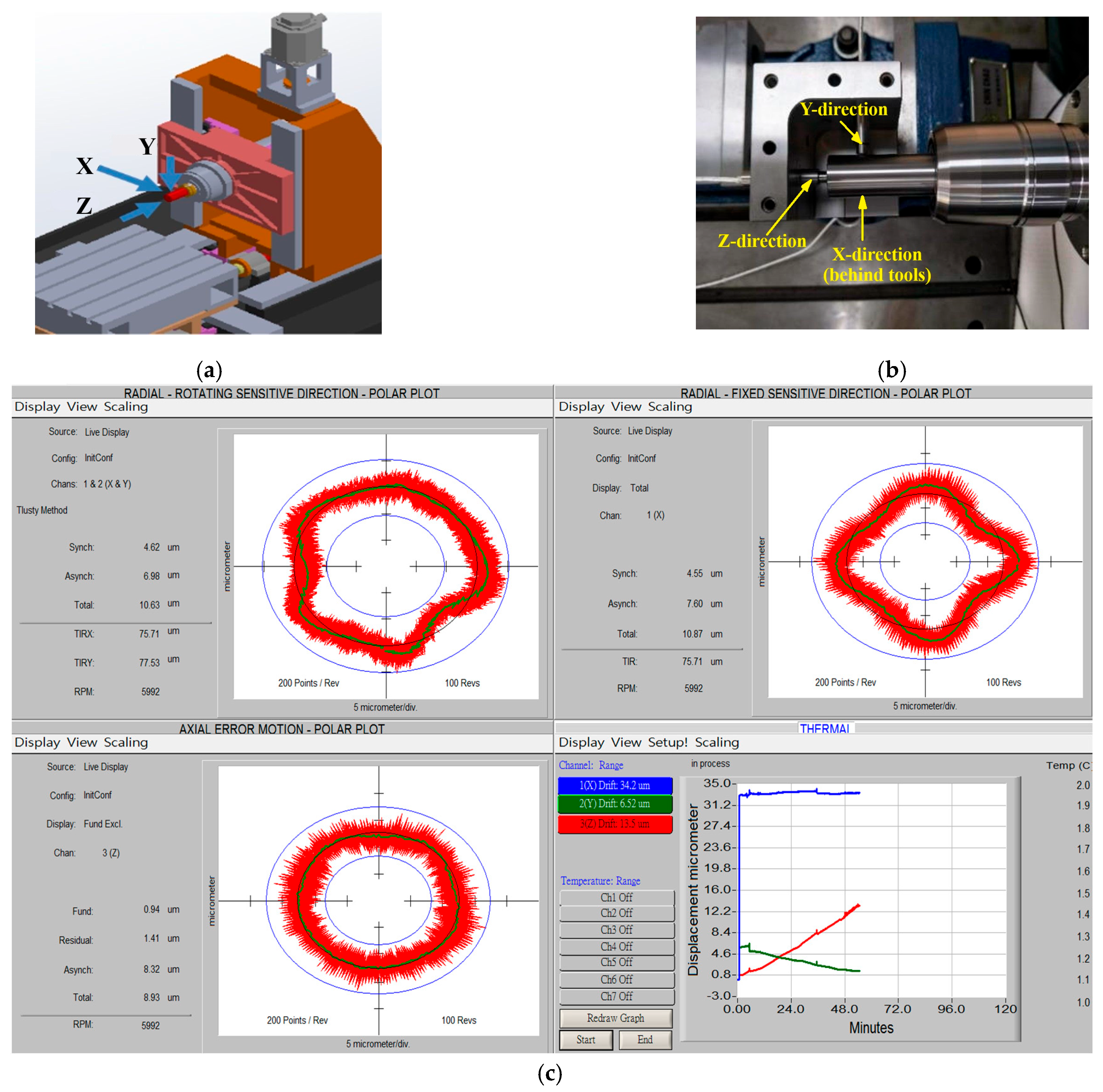
2.1. Experimental Setup

A horizontal milling machine was utilized in this study (Figure 2) to investigate the thermal–mechanical behaviors of the milling spindle under different operating conditions. The main structural components include the spindle, the spindle head ram, the moving column, the worktable, and the machine base. The worktable is mounted on the machine base and driven by a hybrid guide mechanism along the X-axis direction. The column is installed on the machine base and driven through the Z-axis guide mechanism in the horizontal direction. The spindle head ram was installed on the moving column and could be moved along the Y-axis feed in the vertical direction. To improve the rigidity of the spindle head base, the guide rail system is designed and manufactured as a hybrid system of linear roller guide rails and sliding guide rails. The feeding stroke of the X-, Y-, and Z-axes is 300 × 300 × 300 mm. The spindle used was a motorized spindle (EMS 30), in which the spindle shaft was supported by the front and rear bearing pairs coded 7009C and 7006C, respectively. Referring to the bearing manufacturers [42], the geometry information of the 7009C angular ball bearings is given as follows: contact angle (15°), inside diameter (45 mm), outside diameter (75 mm), width (16 mm), ball number (17), and ball diameter (9.55 mm). In this study, the spindle bearings were preloaded at 220 N using positioned spacers and lubricated with grease (SKF LGLT 2), which has a kinematic viscosity of 18 mm2/s at 40 °C [42]. The spindle has a permanent magnetic motor with a rated power of 7.5 KW and torque of 6.1 N·m. Also, the spindle is equipped with a water-cooling jacket around the outer rings of the front bearings and the motor stator. The maximum coolant flow rate is 10 L/min at the initial ambient temperature of 22 °C.
Figure 2 is a schematic diagram of the thermal temperature rise and displacement measurement experiment. The run-in tests were conducted under different spindle speeds, at 3000, 6000, 9000, and 12,000 rpm, respectively. Each run-in test was operated from room temperature up to a stable thermal state, around 3.5 h, for measuring the thermal deformation with the temperature rise.
Temperature measurement instruments generally have combined devices and analysis components. The basic hardware includes T-type thermocouple sensors, a data acquisition module (DAQ NI-9213), and LabVIEW data acquisition software (NI LabVIEW for Education, version 2014). Targets of temperature rise measurements are at the components that generate heat, such as bearings and built-in motors. Direct measurement of the heat source cannot be achieved, since no sensors were embedded in the spindle. Therefore, the temperature sensors were mounted at a position that was as close as possible to the heat generation sources and ambient temperature, as shown in Figure 3. Location indications from T0 to T4 indicate the sensor positions measuring temperature rises at the outer surface of the spindle housing near front bearing 1, front bearing 2, rear bearing, and motor stator, respectively.
The displacements of the spindle tool were measured using the Spindle Error Analyzer (Li-on Precision), which includes noncontact capacitive displacement meters, data acquisition cards, and multi-channel spectrum analysis software, as shown in Figure 4. Three capacitive displacement sensors were mounted on the fixture to measure the axial elongation (Z-axis) and radial deflection (X-axis and Y-axis) of the cylindrical bar fixed with a spindle tool holder, respectively.

2.2. Thermal Deformation Prediction Model: Multivariate Regression Analysis

In this study, multiple linear regression analysis is applied to establish the thermal error model based on experimental measurements, which can be defined as a linear combination of multiple independent variables and one dependent variable [43]. The input features for our multivariate regression models are meticulously selected to capture the thermal state of the motorized spindle. Specifically, these include real-time temperature measurements. Multiple temperature sensors were placed at critical locations on the motorized spindle (bearings and motor housing). These sensors provide continuous, real-time temperature data. The selection of these locations was based on preliminary thermal analysis and practical considerations, ensuring they represent the most influential thermal sources and heat transfer paths affecting spindle deformation. These temperature inputs are the driving forces behind the thermal expansion and subsequent mechanical deformation of the spindle. The output responses of the models directly represent the mechanical behavior resulting from these thermal inputs, providing real-time displacement values. The primary output responses are the real-time displacements of the motorized spindle. These displacements, measured using high-precision sensors, quantify the thermal-induced deformation at specific points on the spindle. These outputs are crucial for understanding the operational stability and precision of the spindle, as excessive or unpredictable displacement can lead to machining inaccuracies.
Equation (1) is a general equation for multivariate regression with standard deviation in Equation (2)
Y = β 0 + β 1 X 1 + β 2 X 2 + + β n X n + S d ( Y )
S d Y = σ ( independent   of   X s )
where Y is a dependent variable, X1Xn are independent variables, β1…βn is the regression coefficient, and σ = σres is the residual standard deviation/error (RSD/RSE). Basically, the regression coefficients can be obtained by using the well-known least-squares method.
In the multivariate regression analysis, we include ANOVA (analysis of variance) to give information about the total variability in Y, which can be partitioned into a part of regression and residual variation. Equation (3) shows the ANOVA Mean Squares (MS) equation:
( Y Y ¯ ) 2 = ( Y f i t Y ¯ ) 2 = ( Y Y f i t ) 2
where Y Y ¯ 2   is the total sum of squares (SSTO), Y f i t Y ¯ 2 is the sum of squares due to regression (SSR), and Y Y f i t 2   is the sum of squares error (SSE).
To explain the goodness of fit for the regression model, the coefficient of multiple determination (R-squared), Root Mean Square Error (RMSE), and model accuracy are used. It is defined as Equations (4)–(6):
R 2 = S S R S S T O = 1 S S E S S T O
R M S E = S S E n
η = 1 i = 1 n Y Y f i t i = 1 n Y f i t
where R2 is the coefficient of multiple determination, SSR is the sum of squares regression, SSTO is the total sum of squares, SSE is the sum of squares error, n is the number of data points, RMSE is the Root Mean Square Error, and η is the model accuracy.
The linear relationship between data expressed by R2 has a value of 0 ≤ R2 ≤ 1. When R2 = 0, it means that the dependent and independent variables do not have a linear relationship, and when R2 ≠ 0, it can be explained by the linear relationship between the dependent and independent variables.

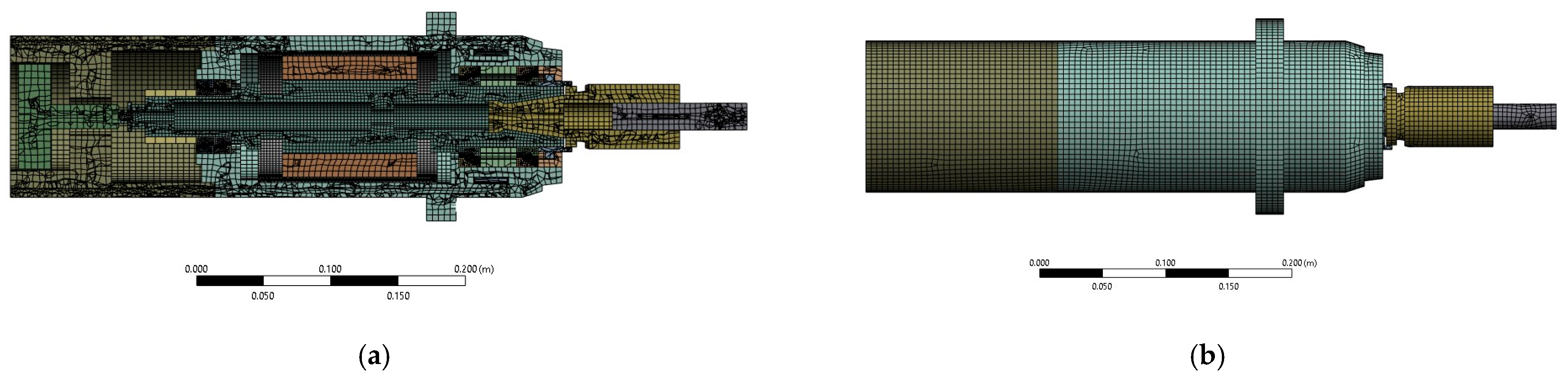
3. Finite Element Modeling Approach

In the FEM approach, there are two modules in thermal analysis, including steady-state thermal and transient thermal analysis. The results from both can be coupled with structural analysis, static and transient. Figure 5 shows the boundary conditions for thermal analysis, including two heat sources from ball bearings and a built-in motor, and 4 convection coefficients (natural convection from ambient temperature, and forced convection from water-cooling channel, rotating parts, and oil/grease lubrication). The heat source of the ball bearing applies to all ball-bearing surfaces, and the heat source of the built-in motor applies to the rotor and stator.

3.1. Thermal–Mechanical Modeling

The thermal error model describes the thermal characteristics and thermal deformation of the spindle tool system under the interactions of the heat source and heat dissipation in operation. The main heat sources of the motorized spindle are bearing heat loss and built-in motor heat losses. Motor heat losses include mechanical heat loss, electric loss, and magnetic loss, while heat dissipation is caused by interaction with the surrounding air and the cooling system through heat transfer in various ways, such as heat conduction and heat convection across the different components. The influence of thermal contact resistance in bearings and bearings with rolling elements can be ignored in the above models because of the difference between the continuum and joint surface heat transfer [44].

3.2. Heat Generation of Ball Bearing

The heat generation in rolling elements, especially in bearings, is influenced by several factors, including the speed at which the bearing operates, the axial load, the radial load, the viscosity of the lubricant used in the bearing, and the moment exerted on the rolling element. However, calculations through the empirical formula of the generated power caused by bearing friction have been summarized by Harris [45], which is written as follows:
H = 1.047 · 10 4 · M · n
where H is the heat with the unit of energy in the form of watts, and M is the sum of the moments composed of mechanical friction torque (Ml) and viscous friction torque (Mv). Ml is determined by the bearing-type load factor f1, bearing load Fβ, and the diameter of the ball bearing dm and is written as follows:
M l = f 1 · F β · d m = z X 0 F r + Y 0 F a C o r y · F a 0.1 F r · d m
where z and y are ball-bearing constants depending on the bearing type and nominal contact angle, and X0 and Y0 are static equivalent loads according to the manufacturer’s data [42]. Fr and Fa are radial and axial forces, respectively; Cor is the static load rating; and dm is the diameter of the ball bearing.
Mv is torque caused by viscous fluid friction. Palmgren, as cited by Harris [45], established an empirical equation as follows:
M v = 10 7 f 0 v 0 n 2 3 d m 3 ,   f o r   v 0 n 2000
M v = 10 7 f 0 d m 3 ,   f o r   v 0 n 2000
where f0 is a factor depending on the arrangement and lubrication method of the bearing, in which f0 = 4 for duplex arrangement with lubrication using grease [46]. vo is the lubricant viscosity (mm2/s), and n is the spindle speed (rpm).

3.3. Heat Generation of Built-In Motor

The heat generation of the motor is mainly related to input power and efficiency, and the input power of the motor can be calculated using Equation (11).
P i n = 3   U s I s c o s φ
Here, Us and Is are the line voltage and the current of the copper winding coil of the stator, respectively, and φ is the motor power factor. The efficiency is determined by the input power and power loss, which normally appear in the form of heat transferred to the surroundings. In general, heat generation includes mechanical loss, electrical loss, and magnetic loss [28]. The heat generation power of the motor can be calculated using Equation (11). The mechanical loss arises from the friction in the air gap between the rotor and stator during high-speed rotation. The mechanical heat loss can be calculated using Equation (12):
P n = π 3 f r 2 D r 3 L r μ a h g
where fr is the rotational frequency of the rotor, Dr is the outer diameter of the rotor, μa is the kinematic viscosity of air, hg is the thickness of the gap between the rotor and stator, and Lr is the rotor’s outer length.
Electric loss is the power loss that occurs when the current passes through the stator conductor coil, which is mainly related to the magnitude of the current. This loss can be calculated using Equation (13):
P e = ρ   I 2 R
where Pe is the electrical power loss in units of watts, ρ is the conductor resistivity, I is the winding current of the stator, and R is the conductor resistance of the stator winding [Ω].
Magnetic loss is the loss formed by the eddy current (Pw) and hysteresis (Ph) of the stator and rotor cores, including eddy current loss and hysteresis loss. This loss can be calculated using Equation (14).
P m = P w + P h = π   δ 2   ( f   B m a x ) 2 6   ρ   r c + C h   f   B m a x a
Here, Pm is the eddy current power loss in watts, δ is the thickness of rotor, f is the magnetic field change frequency, Bmax is the maximum magnetic induction intensity, ρ is the iron core resistivity (Ωm), rc is the iron core density (kg/m3), Ch is a constant related to the rotor material grade, and a is an empirical constant. As noted in the above equations, it is difficult to accurately calculate the electric and magnetic losses and other additional losses of the built-in motor, since many parameters involved in the equations require more experimental work with detailed analysis of the measurements. Therefore, the overall heat-generating power Qm of the motor can be determined by the electric power input to the motor transmission and the mechanical efficiency [44,47], as shown in Equation (15).
Q m = P i n · 1 η · η
Here, Qm is the heat generation from the motor, Pin is the electric input power to the motor, and η and η′ are the mechanical efficiency of the input power to mechanical power and the conversion efficiency of power loss to heat, which were assumed as 0.9 and 0.88 [48] respectively.

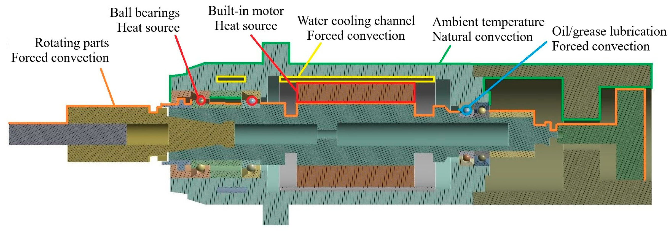
3.4. Convective Heat Transfer Coefficient

Heat transfer phenomena can occur in three forms: conduction, convection, and radiation. The main types of heat transfer occurring in this study are predominantly conduction and convection [46]. The conduction heat transfer coefficient is calculated internally by the software and is included in the properties of a material as thermal conductivity. On the other hand, the convective heat transfer of the entire spindle unit includes two types of convection, free (natural) and forced convection, which are calculated.
The natural heat transfer is caused by the interaction between all stationary components and the ambient air. The natural convection coefficient is given as 9.7 W/m2·°C [49]. The forced convection coefficient heat transfer for rotating components is roughly approximated by using the following formula [50]:
h f = N u · λ D s = 0.133 · R e 2 3 · P r 1 3 · λ D s = 0.133 · u · D s v 2 3 · P r 1 3 · λ D s
where Nu is the Nusselt number, λ is the thermal conductivity of the air in W/m·°C, Re is the Reynolds number, Pr is the Prandtl number of the fluid, which is given as 0.703 for air at room temperature, u is the velocity of the rotating surface, Ds is the equivalent diameter for the rotating components, and v is the kinematic viscosity factor for the fluid in m2/s, which is given as 15.06 × 10⁻⁶ m2/s−1 for air.
The forced convection coefficient heat transfer for the rolling bearing to its lubricants can be estimated using the following equation [51]:
h b = 0.0322 · λ b · P r 1 3 · u s D m v b 1 2
where λb is the heat conductivity of the lubricant (W/m·°C), Pr is the Prandtl number of the grease, us is one-third of the shaft surface velocity of the rotating surface (m/s), Dm is the diameter of the bearing’s outer surface, and vb is the kinematic viscosity factor for the ball-bearing lubricant (m2/s).
The cooling system used in the motorized spindle is composed of cooling water jackets implemented around the front bearings, motor stator, and rear bearings. The heat generated by the built-in motor and bearing was taken out in the form of forced convection by coolant flowing through the cooling channels. The convection coefficient of the water-cooling channel is estimated using the following equation [52]:
h f = N u · λ w L c = 0.023 · R e 0.8 · p r 0.4 · λ w L c = 0.023 · V f · D c   μ   0.8 · P r 0.4 · λ w L c
In which λw and Pr are the thermal conductivity and Prandtl number of the water coolant, which were given as 0.598 W/m·°C and 6.9, respectively. Vf is the average flow rate of cooling water in m/s. Re is the Reynolds number of the coolant flowing through the channel. Dc and Lc are the equivalent diameter and characteristic length of the cooling channel, respectively, which are given as 100 mm and 4945 mm in this study. µ is the kinematic viscosity of the coolant at room temperature, given as 0.89 × 10⁻⁶ m2/s.

3.5. Transient Thermal–Mechanical Analysis

Thermo-mechanical transient analysis considers both thermal effects and mechanical deformation within a system over time. The key to accurate thermo-mechanical analysis effectively depended on the coupling effects of the thermal and structural domains. For spindle systems, considering thermal–structural coupling effects is essential for accurately analyzing time-varying characteristics of heat sources and thermal boundary conditions [53]. Transient thermal analysis is performed by employing a set of governing equations that delineate heat transmission mechanisms, including conduction, convection, and radiation [54]. Meanwhile, transient structural analysis is performed by utilizing the results from the transient thermal analysis to compute the transient deformation in the modules while accounting for mechanical boundary conditions.
The finite element model of the milling spindle is shown in Figure 6. In order to consider the heat transfer across bearing components in thermal analysis, front and rear bearings were included in the spindle unit, which were modeled in 3D elements, including inner and outer races and balls. Basically, the bearing preload was determined by the interferences or clearances among these components. Therefore, these mating components were assumed at rough contact modes with appropriately defined interferences [6,7]. All the structural components were meshed using an 8-node hexahedron and a 10-node tetrahedral element, consisting of 198,090 elements and 759,537 nodes. The materials used for structural components are made of carbon steel with an elastic modulus E = 200 GPa, Poisson’s ratio υ = 0.3, and density ρ = 7800 Kg/m3.

3.6. Thermal Analysis Parameters

Table 1 shows heat loss in watts for the motorized spindle at different spindle speeds. The heat loss is calculated using the equations in Section 3.2 and Section 3.3. The table shows the heat loss for each component: front and rear bearings and built-in motor. It clearly shows that the heat generation of bearings and motor increases significantly when the spindle speed increases from 3000 to 12,000 rpm.
Table 2 presents the convective heat transfer coefficients for different spindle speeds (measured in rpm). It includes four categories: natural convection for stationary parts, forced convection at surfaces of rotating components such as rolling bearings, and forced convection from water-cooling channels. The natural convection coefficient remains constant at 9.7 W/m2·°C across all spindle speeds. The forced convection coefficients for rotating part surfaces, rolling bearing with lubricant, and water-cooling channels all show an increasing trend with an increasing spindle speed. Notably, the water-cooling channel remains consistently high at 202 W/m2·°C.

4. Results and Discussion

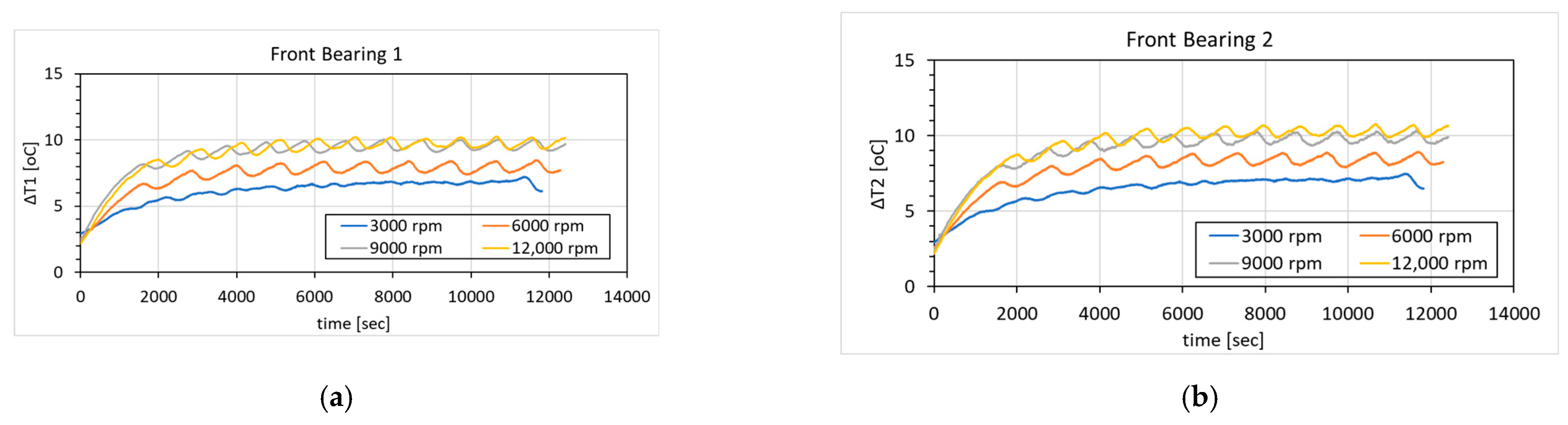
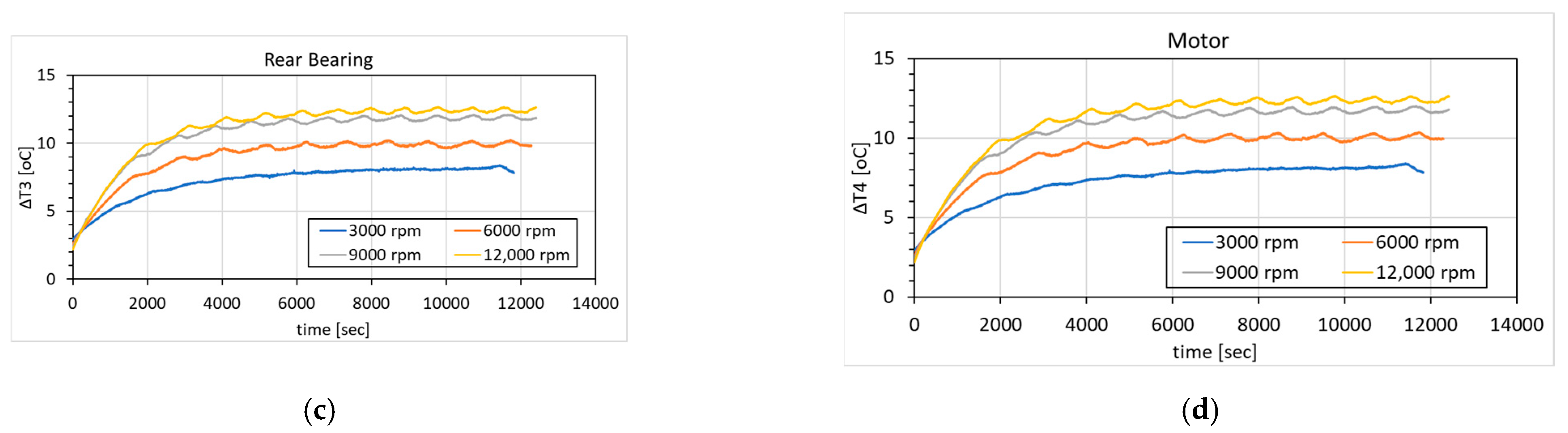
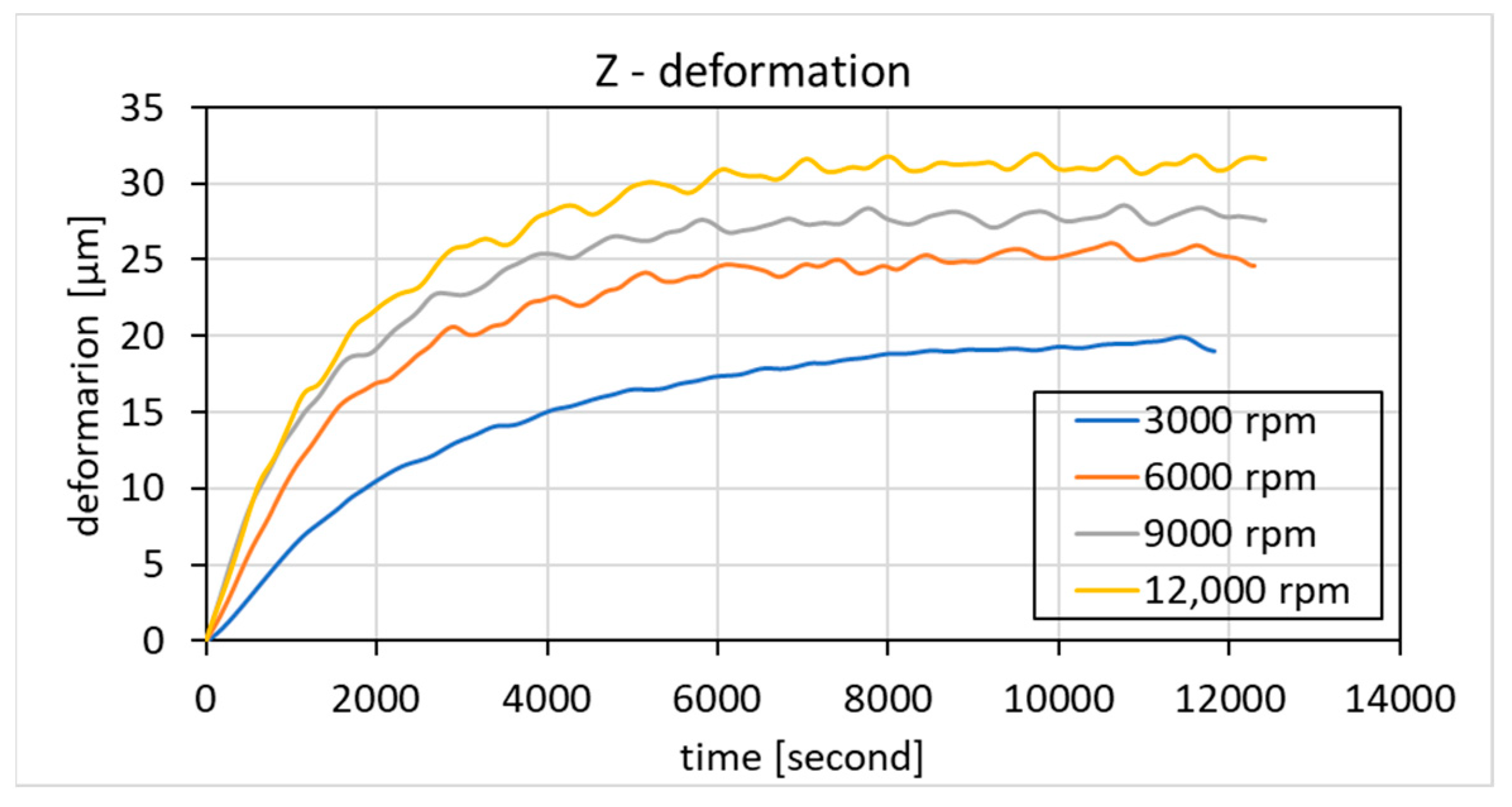
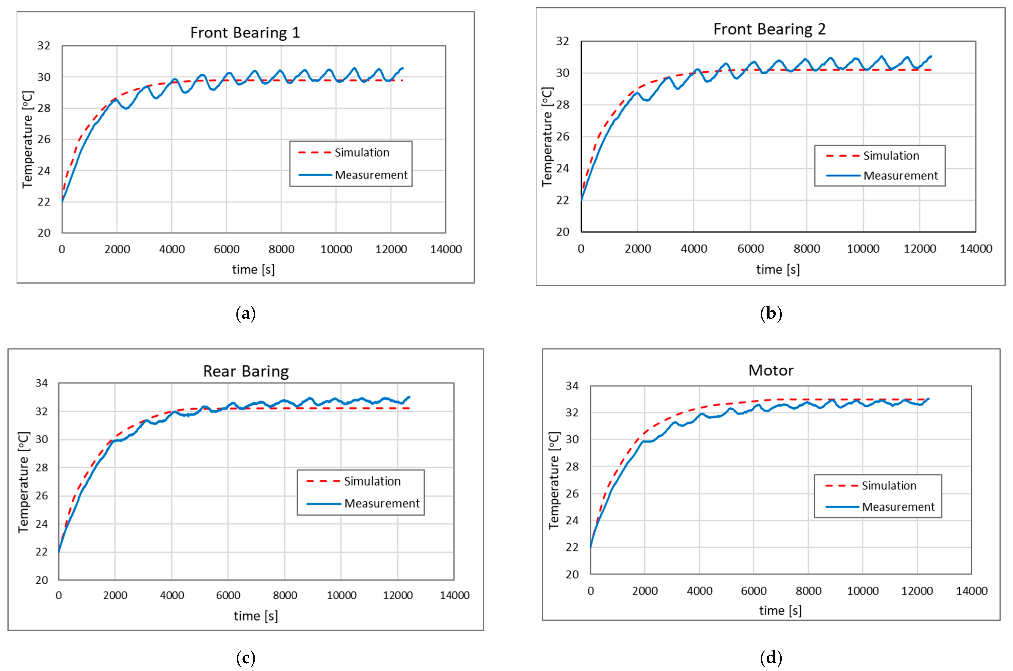
4.1. Thermal Temperature Rise and Deformation Measurement Results

The configuration of sensing elements has a considerable impact on the accuracy of acquiring temperature field data of the machine’s main spindle and establishing mathematical models. Temperature sensing is basically based on the location of the heat source. However, considering the number of temperature sensing components and maintenance costs in later practical applications, it is necessary to reduce the number of sensing components as much as possible without losing accuracy. Therefore, multiple temperature sensing elements (such as T0 to T8) were used in the initial study. After experimental evaluation, the ones with higher relative coefficients for axial elongation were left at locations that are prone to thermal deformation, such as the spindle head, spindle motor, and bearings. The front and rear bearings of the main spindle and the base are the measurement points. The displacement sensing elements are respectively arranged at the tool, which directly affects the processing precision. After a series of experiments, it is found that the one with the highest correlation coefficient for the axial displacement is the front bearing, rear bearing, and motor, so this study uses five sensors (T0~T4). In addition, the relative coefficient of the heating element configured in the motor is the highest, so in the regression analysis part, multiple and single variables are used to bring in predictions to find the best mathematical prediction equation.
Figure 7 illustrates the measured temperature rise of the spindle tool system at four locations: two front bearings, one rear bearing, and the motor. The measurements included various operating speeds from 3000 to 12,000 rpm and were performed over a total time of approximately 3.3 h (12,000 s). The temperature change pattern is shown to be typical for each location, which increases steeply at the initial phase and then slightly increases towards steady-state conditions. In all cases, higher rotational speeds yield a larger increment of temperature than those measured at lower speeds. For example, temperature changes of 10–12 °C were generated at a spindle speed of 12,000 rpm, while at 3000 rpm, an increase in temperature of 5–7 °C was generated. Thermal characteristics of the front bearings are amazingly identical, demonstrating balanced temperature fields as compared to the rear bearing and motor, which generally appear to show slightly elevated temperature rises over the front bearings at higher speeds. At all measured points, it is shown that the temperature slowly rises over time with a tiny fluctuation because of the activation and deactivation of the cooling system at a defined temperature state.
Figure 8 shows the axial thermal deformation behavior during temperature rise under different rotational speeds: 3000, 6000, 9000, and 12,000 rpm. The evolution of the global deformations displays a characteristic trend—fast growth in the former phase and subsequent asymptotical approach to some steady-state levels—with higher rotational velocities always yielding larger total deformation. The maximum deformation (approx. 30–32 μm at 12,000 rpm (yellow line) and only approx. 20 μm at 3000 rpm (blue line) reaches different values under various speeds; furthermore, the spindle tool exhibits different rates of deformation with time. Under higher speed conditions, the axial deformation shows a steeper initial slope and rapidly reaches its near-steady-state conditions as compared to lower speed conditions. The curves indicate that the Z-axis thermal deformation rate and value both correlate consistently with the rotational speed.

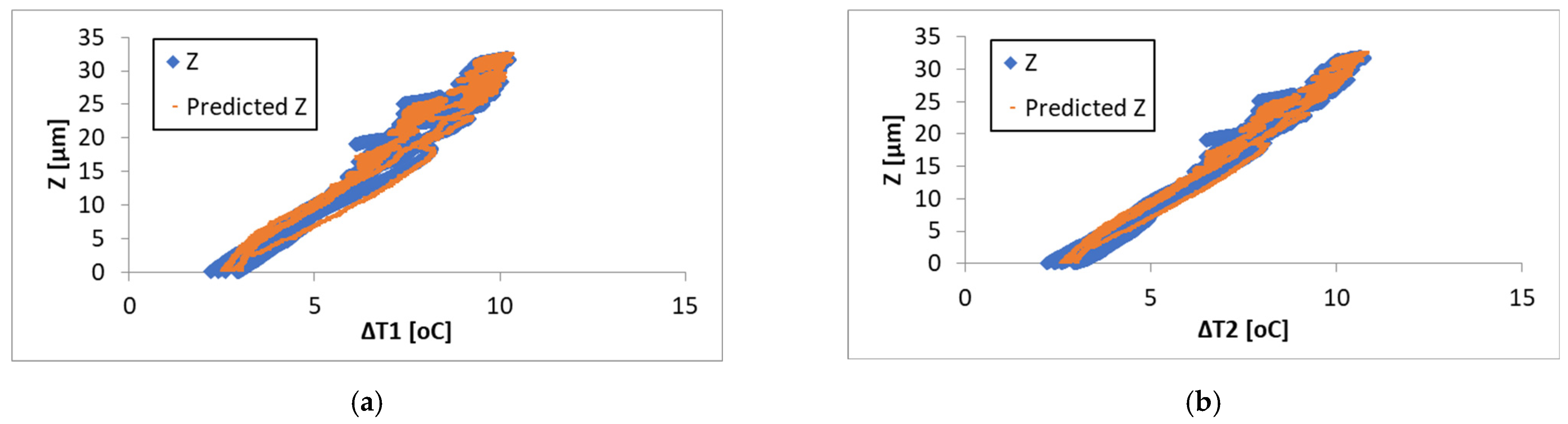
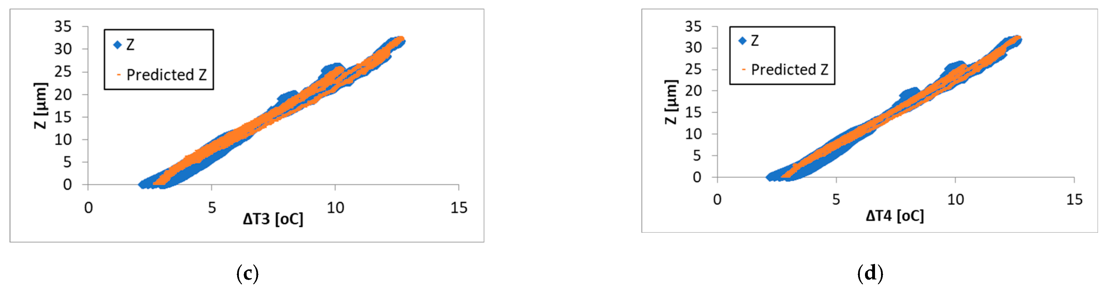
4.2. Multivariate Regression Analysis and Model Selection

During the analysis, the thermal deformation and the temperature rise histories at multiple points were first used as the parameters of the regression analysis, and the correlation coefficients between the temperature rises at different points and the thermal deformation measured at the end of the spindle tool holder were observed. The greater the correlation, the greater the thermal deformation is affected by the temperature rise at this temperature point. If the error between the regression value and the actual measurement value is smaller, this temperature point can be included in the error model. The input end is based on the relative temperature gradient corresponding to five sets of rotation speeds (each sensor deducts the ambient temperature, such as T4-T0), and the output end is the axial temperature rise. Multivariable and single-variable regression analyses are performed to obtain a thermal error prediction model.
Table 3 summarizes the examination of multivariable regression combinations between temperature differences (ΔT1 to ΔT4) as variables and their predictive performance using the residual mean squared error (RMSE), adjusted R-squared (R2) values, ANOVA Mean Squares (MS) values, and model accuracy (η). The analysis looks at single-variable (rows 1–4) to four-variable combinations (row 15), and for each, their RMSE value in micrometers, R2 value, MS values, and their corresponding model accuracy are shown. Generally, with the increase in variables from 1 to 4, the RMSE becomes lower, R2 values are higher, MS are lower, and η are highest. The four-variable model (ΔT1–ΔT2–ΔT3–ΔT4) has the lowest RMSE of 0.8394 μm, the highest R2 value of 0.9871, as well as the lowest MS of 0.7048. For the single-variable model, ΔT4 comes out on top at 1.1162 μm, 0.9772, 1.2459, and 97.11% for the RMSE, R2, MS, and η, respectively.
From Table 3, It can be concluded that the four variables are the best model with the lowest error prediction, highest R2, lowest MS, and highest model accuracy. Among the four selected models, the single variable is the worst model; however, the model accuracy is still acceptable, being more than 95%. Equations (16)–(19) show the mathematical prediction equation for the best model in their groups: one, two, three, and four variables, respectively.
Δ Z ( t ) = 8.021 + 3.156   Δ T 4 ( t )
Δ Z ( t ) = 9.623 7.555   Δ T 3 ( t ) + 10.882   Δ T 4 ( t )
Δ Z ( t ) = 9.106 5.536   Δ T 1 ( t ) + 6.795   Δ T 2 ( t ) + 2.013   Δ T 4 ( t )
Δ Z ( t ) = 9.310 4.077   Δ T 1 ( t ) + 4.854   Δ T 2 ( t ) 2.897   Δ T 3 ( t ) + 5.392   Δ T 4 ( t )
Here, ΔZ(t) represents the axial deformation of the spindle tool holder with temperature rise during run-in tests. ΔT1(t), ΔT2(t), ΔT3(t), and ΔT4(t) represent the increment of temperature of the spindle housing at the points around front bearings, rear bearings, and motors. Each coefficient derived from regression analysis represents the expected change in ΔZ(t) for a one-unit increase in its corresponding predictor, assuming all other predictor variables are held constant. Coefficients of every variable mean that every changing value in the variable will be gained by a multiple of the coefficient. The negative value of the coefficient means that the value of the response variable will decrease.
To contextualize the findings, multivariate regression in this study is comparable with established approaches such as Deep Extreme Learning Machine (DELM), Adaptive Chaos Particle Swarm Optimization (ACPSO), and Beetle Antennae Search Algorithm–Back Propagation (BAS-BP). Table 4 summarizes the key characteristics and performance metrics of our method in comparison to several prominent techniques in the literature.

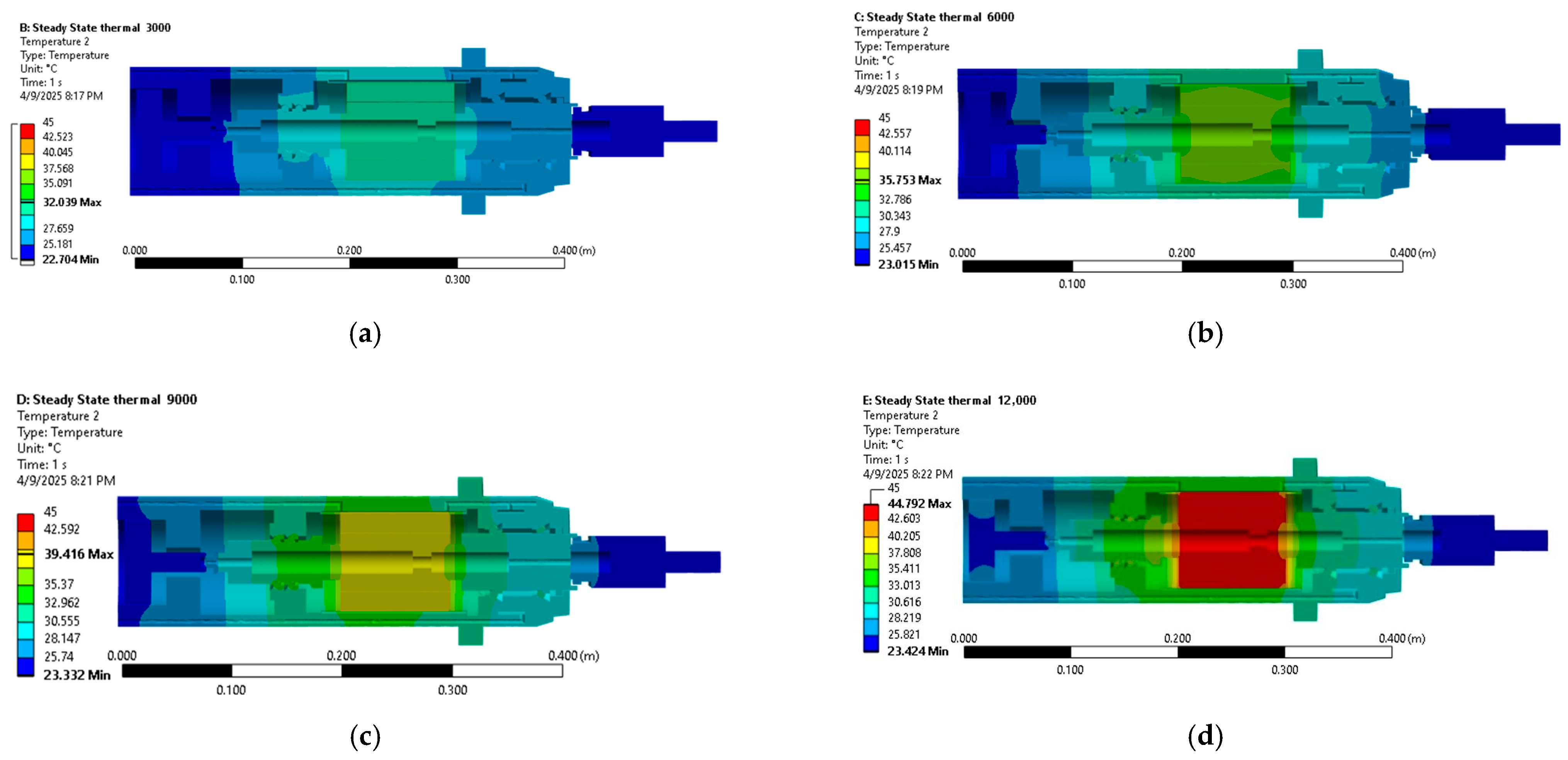
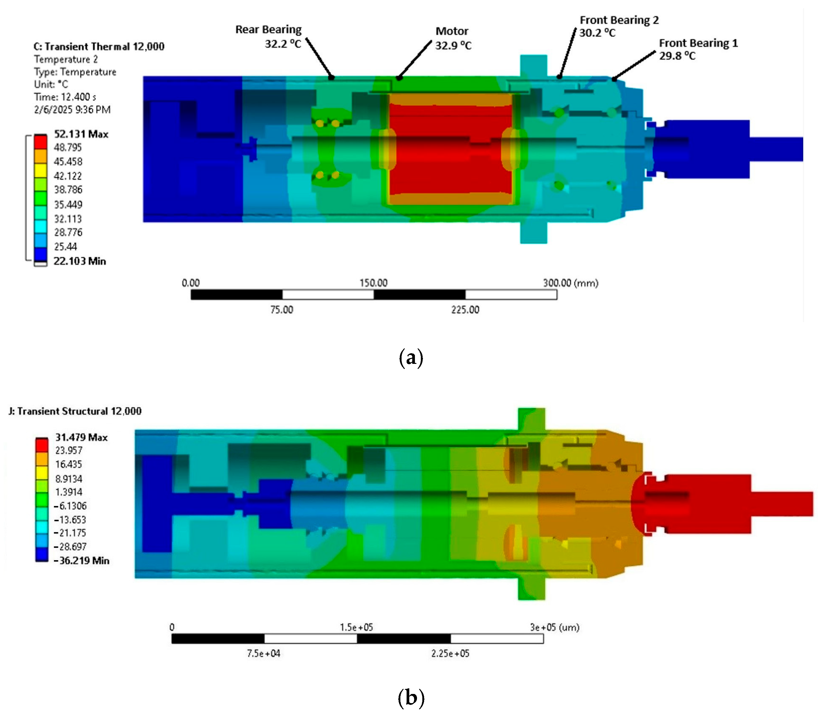
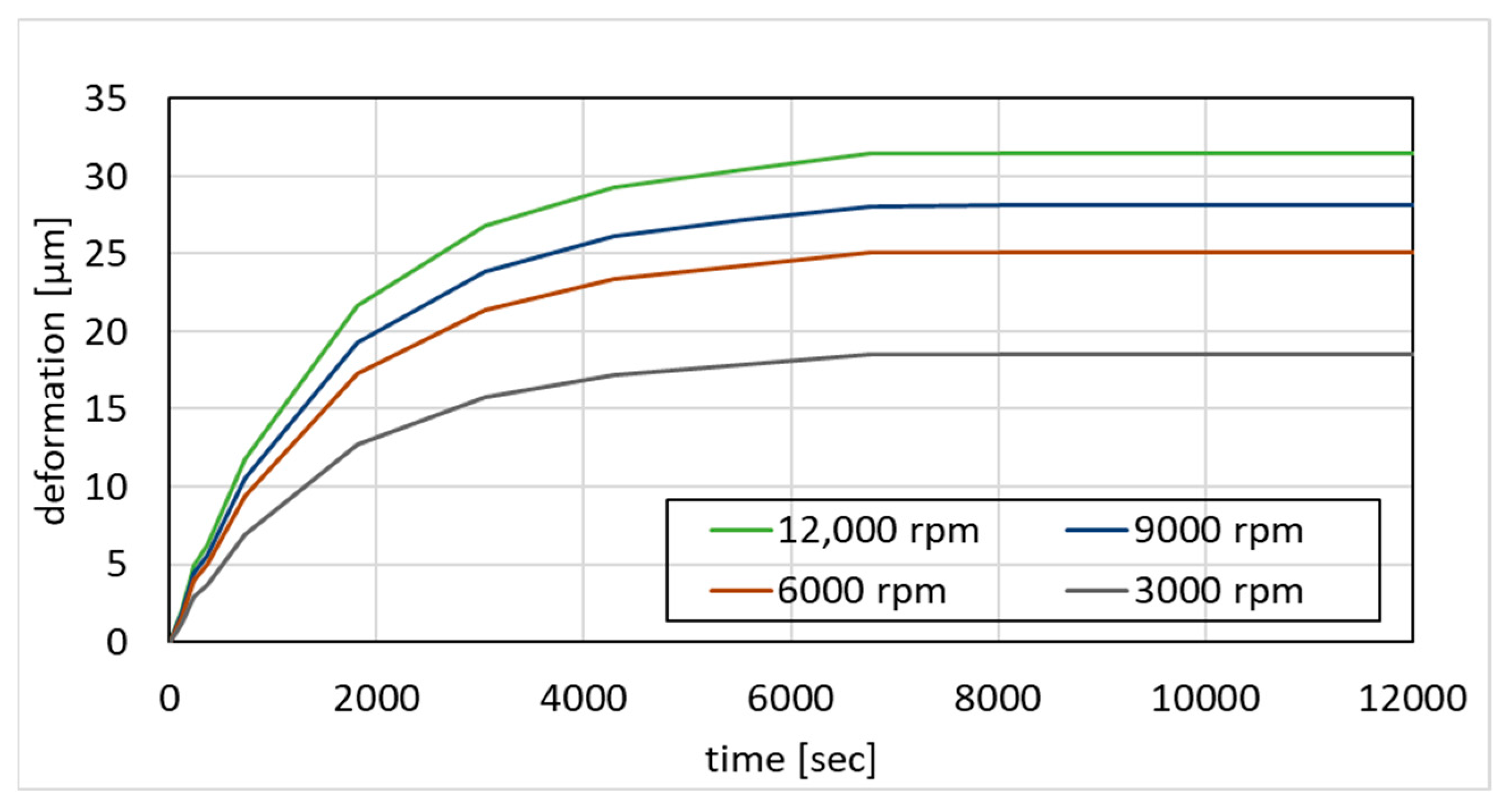
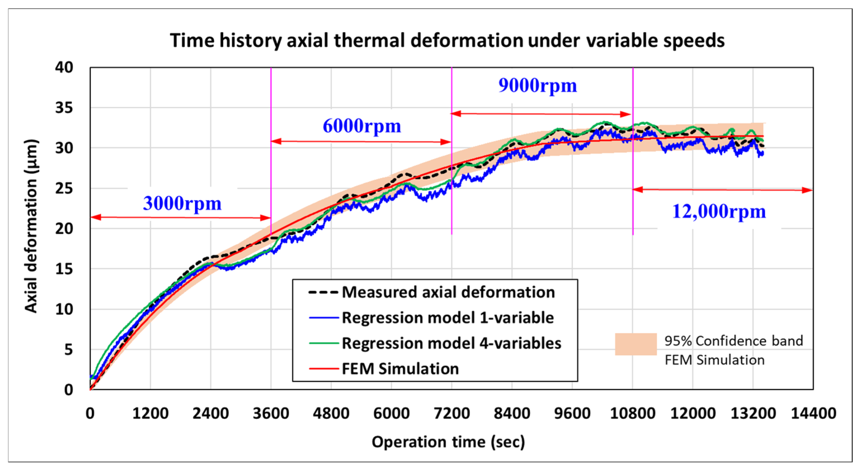
4.3. Thermal–Mechanical Behaviors

The temperature rise feature at the measured positions was validated using the FEM approach, which is comparable to the simulation model. Based on the calculations of heat generation, the heat loss at 12,000 rpm of the front bearing, rear bearing, and motor are 198.6 watts, 76.9 watts, and 317 watts, respectively. The model also includes a convection coefficient in the form of natural convection for free-surface contact with the surroundings; the forced convection includes rotating parts, ball bearings, and water-cooling channels. Steady-state thermal analysis results show that thermal distribution mostly starts from the main heat sources built-in motor and bearings and then spreads to the spindle surface where the possible sensors are placed. Figure 9 shows the difference in temperature distribution at steady-state conditions at different spindle speeds. The maximum temperatures are located at the built-in motor at 32.04, 35.75, 39.42, and 44.79 °C for spindle speeds of 3000, 6000, 9000, and 12,000 rpm, respectively.
Figure 10 shows the temperature distributions of the motorized spindle system predicted through transient thermal simulation at the end of time 12,000 s. The temperature is distributed across the system with components annotated (front bearings, rear bearings, and motor). The temperature unit is colored from 22.1 to 52.1 °C, with red for warmer areas and blue for cooler areas. At the measured locations, it can be seen that the temperatures at front bearing 1, front bearing 2, rear bearing, and motor are 29.8, 30.2, 32.2, and 32.9 °C, respectively. Figure 11 shows the predicted transient temperature rises at the spindle housing under 3000, 9000, 12,000, and 15,000 rpm, which were compared with the measured temperature rises. As observed, the temperature rise histories predicted at different points agree well with the measurements. The observation verifies the accuracy of the digital model of the spindle tool system in predicting thermal behaviors. In addition, the transient thermal simulation results have 14 points with different values simultaneously. All temperature distribution data are then used in structural transient analysis to calculate deformation for each of the 14 specific time-based temperature distribution loads.
Table 5 presents axial thermal deformation from transient analysis simulation, which consists of the time-step data, input thermal data at observed points, and z-deformation at different spindle speeds. There are 15 steps along an observed time of up to 12,400 s, each lasting around 120 s. Transient thermal analysis results, as distributed temperature, are then imported to the transient structural analysis for every step. The result of the transient structural analysis is presented in deformation in the z-direction (along with the spindle axis). As illustrated in Figure 12, the deformation increases over time for each spindle speed. The graph indicates that the deformation curve for the highest speed (12,000 rpm) rises the most steeply, followed by 9000 rpm, 6000 rpm, and 3000 rpm, confirming that faster spindle speeds cause greater deformation. The steady-state time is reached after about 8000 s. At the end of the time (around 12,000 s), the deformation values for the highest spindle speed (12,000 rpm) reach around 30 µm, while the lowest spindle speed (3000 rpm) results in a deformation close to 20 µm.

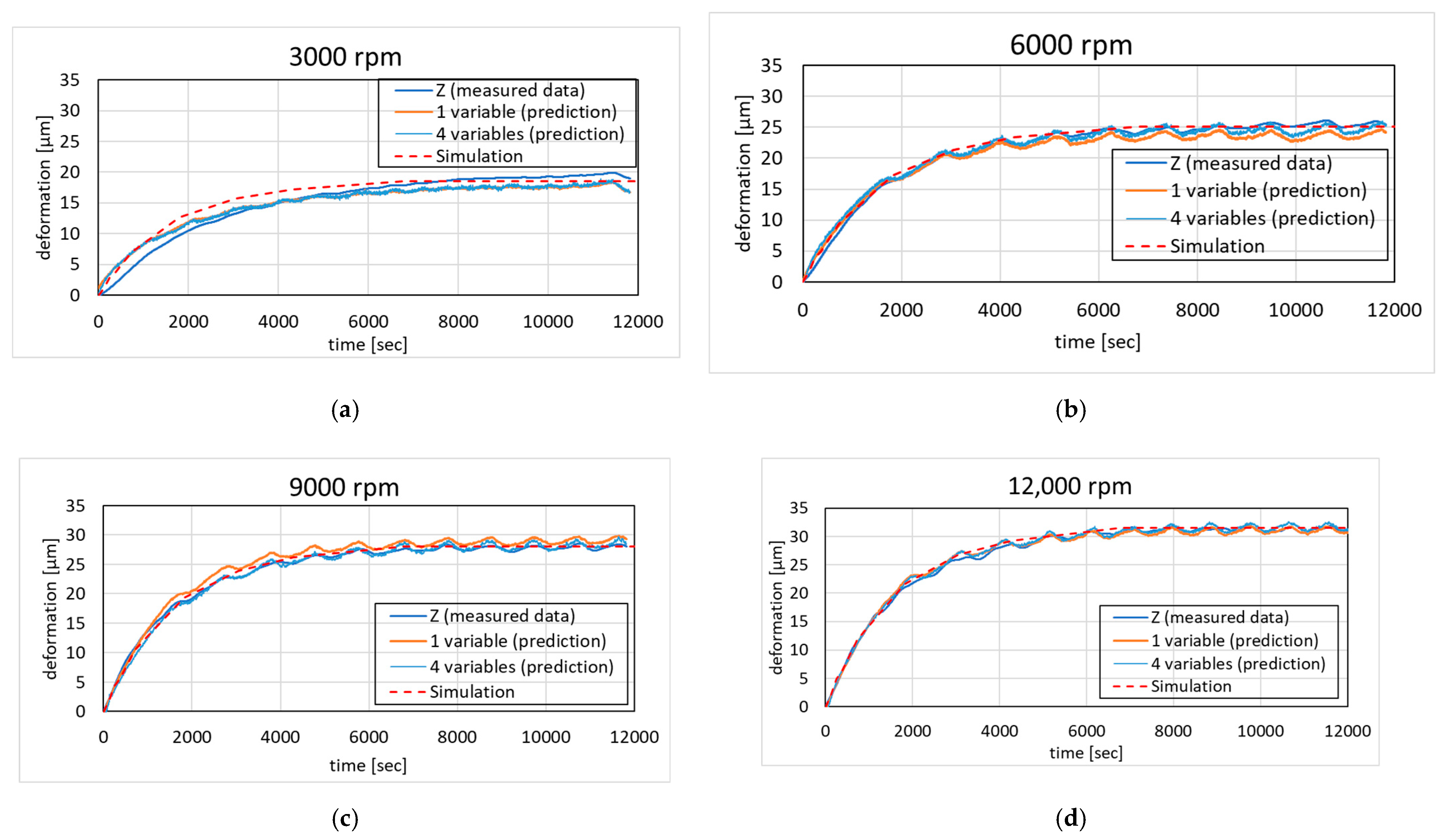
4.4. Model Verification

The prediction performances of the thermal error regression models were evaluated by comparing the predicted values and measured deformation under different speeds, which can be quantified using the RMSE, as listed in Table 6. Generally, the maximum error decreases with an increasing spindle speed, with an RMSE range of 1.299 to 1.450 µm at 3000 rpm and 0.500 to 0.586 µm at 12,000 rpm. It is clear that the temperature rise predicted by the regression models with a single variable and multiple variables is comparable to the measurements. The observation verifies the accuracy of the regression thermal error models in predicting thermal behaviors.
The transient thermal–mechanical behaviors of the spindle tool can also be well simulated using a finite element modeling approach. The results of the FE simulation were also illustrated in Figure 13, which presents the Z-axis deformation values at four different rotational speeds (3000, 6000, 9000, and 12,000 rpm) over a period of 12,000 s. Comparisons of the predicted time history of the axial deformation with the experimental measurements and regression predictions are demonstrated in Figure 13. In each subplot, the measured data (blue line) as well as a single-variable prediction model (orange line), a four-variable prediction model (thin blue line), and a finite element model (green line), are compared. The results showing the predicted time histories of thermal deformations are in good agreement with the measurements, which revealed variations in the thermal deformation of the same tendency, a rapid increase at the initial phase with an increasing temperature with time, and then a mild growth to a stable state with maximum deformation (about 20 μm at 3000 rpm versus 32 μm at 12,000 rpm). The prediction model seems to match the measured data best at 12,000 rpm, which agrees with the reported lower maximum error value for this speed. The prediction model is a reasonably close match to the data for all speeds, although there are some small discrepancies with the measured data, especially in steady-state regions.
Further validations were carried out by conducting additional experiments with run-in operation under variable speeds. The axial deformation over time at different speeds was measured, which included operation under speeds of 3000, 6000, 9000, and 12,000 rpm at four different time periods, that is, 0–3600, 3600–7200, 7200–10,800, and 10,800–14,400 s, accordingly, as shown in Figure 14. As the spindle speed increases, the deformation rises in distinct steps, with each step corresponding to a change in the spindle speed after one hour of operation. Axial thermal deformation increases rapidly at 3000 rpm and reaches about 18 µm at the end of time, showing a transient status. During the period from 3600 to 7200 s with a spindle speed of 6000 rpm, deformation rises gradually from around 18 µm to around 27 µm, with small fluctuations, indicating that it is still in the transient period. At times, in the region of 7200–14,400 seconds and at a spindle speed of 9000 to 12,000 rpm, the deformation changes steadily, with fluctuations reaching approximately 28 µm and 32 µm, respectively. In comparison with the results of finite element thermal–mechanical analysis, the structural transient simulation was conducted continuously by importing the thermal loads yielded from thermal transient analysis, which depend on the operation conditions of the spindle speed and time period assumed in the transient analysis. In addition, three regression thermal error models (one variable and four variables) are compared with the measured data for different time periods. The four-variable regression prediction and FE simulation have a prediction error and RMSE of 0.84 and 0.82 µm, respectively, which closely agree with the measurements, comparable to the increasing tendency of the thermal deformation with time in each operation condition. The one-variable prediction with an RMSE of 1.33 µm shows the general trend but deviates more from the measured data, especially during transitions between spindle speeds. The simulation results generally have a trend comparable to the measurements and regression predictions, with a 95% confidence level band, although at 3000 rpm, lagging behind the others. Overall, higher spindle speeds result in greater axial deformation, and the multivariable models and finite element models provide more accurate predictions of the transient thermal–mechanical behaviors, as demonstrated in real experimental scenarios.
Figure 15 shows the results of a prediction model verification analysis. The line fit plot demonstrates the relationship between the ΔT (temperature change) and axial deformation measurements, where the actual data points (in blue) closely follow the predicted values (in orange), suggesting a strong linear correlation. The plot shows the difference between observed and predicted values across the temperature range, with residuals mostly falling within ±1.2 μm and displaying a somewhat irregular pattern that appears to have increasing variance at higher temperatures. Figure 15d shows that ΔT4 (temperature change at motor) has a smaller variance than the others, meaning that ΔT4 significantly influenced the model. The ΔT4 variable also indicates the best model for a single-variable model.

5. Conclusions

This study presented an integrated approach for analyzing and predicting the thermal–mechanical behavior of motorized spindles using experimental measurements, regression analysis, and finite element (FE) simulation. A strong correlation was confirmed between temperature rise and axial deformation, enabling accurate modeling of thermal error under varying operating conditions.
Rather than simply highlighting prediction accuracy, this work emphasizes the practical benefit of sensor count reduction. The findings show that a single, strategically placed sensor can still achieve reliable thermal deformation prediction with minimal loss in accuracy. This has significant implications for industrial applications, where reducing the number of sensors not only lowers the system complexity and cost but also improves the maintainability, robustness, and integration potential in commercial machine tools.
Moreover, the validated FE model offers a scalable digital foundation for further development of real-time compensation systems and digital twin frameworks, allowing manufacturers to implement predictive control strategies without extensive physical testing. This methodology contributes directly to improving the precision, reliability, and cost effectiveness of spindle systems in high-speed, high-precision machining environments. Future work may focus on integrating this approach with adaptive control systems, expanding to multi-axis error modeling, or leveraging the FE model for training machine learning algorithms in hybrid prediction frameworks.

Author Contributions

Conceptualization and methodology, T.M.A., W.-Z.L., Y.-J.C. and J.-P.H.; software and formal analysis, T.M.A., W.-Z.L., Y.-J.C. and M.A.R.; investigation, T.M.A., W.-Z.L., Y.-J.C. and M.A.R.; resources, J.-P.H.; data curation, T.M.A., W.-Z.L. and M.A.R.; writing—original draft preparation, T.M.A. and W.-Z.L.; writing—review and editing, J.-P.H.; visualization, T.M.A. and W.-Z.L.; supervision, J.-P.H.; project administration, J.-P.H.; funding acquisition, J.-P.H. All authors have read and agreed to the published version of the manuscript.

Funding

This research was funded by the National Science and Technology Council, Taiwan, R.O.C., under grant numbers MOST 108-2622-E-167-020-CC3 and NSTC 2221-E-167-021.

Data Availability Statement

Data are contained within the article.

Acknowledgments

We gratefully acknowledge the support for this work provided by Posa Machinery Co., Ltd. Taiwan.

Conflicts of Interest

The authors declare no conflicts of interest.

References

  1. Fu, Y.Q.; Gao, W.G.; Yang, J.Y.; Zhang, Q.; Zhang, D.W. Thermal Error Measurement, Modeling and Compensation for Motorized Spindle and the Research on Compensation Effect Validation. Adv. Mater. Res. 2014, 889–890, 1003–1008. [Google Scholar] [CrossRef]
  2. Lei, M.; Gao, F.; Li, Y.; Xia, P.; Wang, M.; Yang, J. Feedback Control–Based Active Cooling with Pre-Estimated Reliability for Stabilizing the Thermal Error of a Precision Mechanical Spindle. Int. J. Adv. Manuf. Technol. 2022, 121, 2023–2040. [Google Scholar] [CrossRef]
  3. Zhang, Y.; Liu, T.; Gao, W.; Tian, Y.; Qi, X.; Wang, P.; Zhang, D. Active Coolant Strategy for Thermal Balance Control of Motorized Spindle Unit. Appl. Therm. Eng. 2018, 134, 460–468. [Google Scholar] [CrossRef]
  4. He, S.; Tang, T.; Bao, J.; Tang, R. Research on Teaching Reform of Experimental Measurement of Temperature Field and Thermal Deformation of Machine Tool. IOP Conf. Ser. Earth Environ. Sci. 2019, 358, 042015. [Google Scholar] [CrossRef]
  5. Prasad, V.V.S.H.; Kamala, V. Thermal Error Compensation in High-Speed CNC Machine Feed Drives. AIP Conf. Proc. 2021, 2317, 030026. [Google Scholar] [CrossRef]
  6. Arief, T.M.; Liao, H.-E.; Lin, P.-Y.; Hung, J.-P. Finite Element Modeling of Milling Spindle Thermal Behavior with Variation of Bearing Preload. In Lecture Notes in Mechanical Engineering; Springer: Singapore, 2025; pp. 439–446. [Google Scholar] [CrossRef]
  7. Arief, T.M.; Lin, W.-Z.; Royandi, M.A.; Hung, J.-P. Development of a Digital Model for Predicting the Variation in Bearing Preload and Dynamic Characteristics of a Milling Spindle under Thermal Effects. Lubricants 2024, 12, 185. [Google Scholar] [CrossRef]
  8. Li, Y.; Zhao, W.; Lan, S.; Ni, J.; Wu, W.; Lu, B. A Review on Spindle Thermal Error Compensation in Machine Tools. International J. Mach. Tools Manuf. 2015, 95, 20–38. [Google Scholar] [CrossRef]
  9. Liu, K.; Liu, H.; Li, T.; Liu, Y.; Wang, Y. Intelligentization of Machine Tools: Comprehensive Thermal Error Compensation of Machine-Workpiece System. Int. J. Adv. Manuf. Technol. 2019, 102, 3865–3877. [Google Scholar] [CrossRef]
  10. Li, Y.; Yu, M.; Bai, Y.; Hou, Z.; Wu, W. A Review of Thermal Error Modeling Methods for Machine Tools. Appl. Sci. 2021, 11, 5216. [Google Scholar] [CrossRef]
  11. Liu, H.; Miao, E.; Wang, J.; Zhang, L.; Zhao, S. Temperature-Sensitive Point Selection and Thermal Error Model Adaptive Update Method of CNC Machine Tools. Machines 2022, 10, 427. [Google Scholar] [CrossRef]
  12. Yao, X.; Hu, T.; Yin, G.; Cheng, C. Thermal Error Modeling and Prediction Analysis Based on OM Algorithm for Machine Tool’s Spindle. Int. J. Adv. Manuf. Technol. 2020, 106, 3345–3356. [Google Scholar] [CrossRef]
  13. Yue, H.; Guo, C.; Li, Q.; Zhao, L.; Hao, G. Thermal Error Modeling of CNC Milling Machining Spindle Based on an Adaptive Chaos Particle Swarm Optimization Algorithm. J. Braz. Soc. Mech. Sci. Eng. 2020, 42, 427. [Google Scholar] [CrossRef]
  14. Wei, X.; Ye, H.; Miao, E.; Pan, Q. Thermal Error Modeling and Compensation Based on Gaussian Process Regression for CNC Machine Tools. Precis. Eng. 2022, 77, 65–76. [Google Scholar] [CrossRef]
  15. Fu, G.; Mu, S.; Zheng, Y.; Lu, C.; Wang, X.; Wang, T. MA-CNN Based Spindle Thermal Error Modeling Using the Depth Feature Analysis with Thermal Error Mechanism. Measurement 2024, 226, 114183. [Google Scholar] [CrossRef]
  16. Li, Z.; Zhu, B.; Dai, Y.; Zhu, W.; Wang, Q.; Wang, B. Research on Thermal Error Modeling of Motorized Spindle Based on BP Neural Network Optimized by Beetle Antennae Search Algorithm. Machines 2021, 9, 286. [Google Scholar] [CrossRef]
  17. Dai, Y.; Pang, J.; Rui, X.; Li, W.; Wang, Q.; Li, S.-Z. Thermal Error Prediction Model of High-Speed Motorized Spindle Based on Delm Network Optimized by Weighted Mean of Vectors Algorithm. Case Stud. Therm. Eng. 2023, 47, 103054. [Google Scholar] [CrossRef]
  18. Liu, Y.-C.; Li, K.-Y.; Tsai, Y.-C. Spindle Thermal Error Prediction Based on LSTM Deep Learning for a CNC Machine Tool. Appl. Sci. 2021, 11, 5444. [Google Scholar] [CrossRef]
  19. Wei, X.; Ye, H.; Wang, G.; Hu, W. Adaptive Thermal Error Prediction for CNC Machine Tool Spindle Using Online Measurement and an Improved Recursive Least Square Algorithm. Case Stud. Therm. Eng. 2024, 56, 104239. [Google Scholar] [CrossRef]
  20. Zhang, Y.; Liu, Z.; Liu, Q.; Wang, D.; Li, X. A Comprehensive Prediction and Compensation Method of Spindle Thermal Error for a CNC Grinding Machine. Digit. Eng. 2024, 2, 100012. [Google Scholar] [CrossRef]
  21. Dong, Y.; Chen, F.; Lu, T.; Qiu, M. Research on Thermal Stiffness of Machine Tool Spindle Bearing under Different Initial Preload and Speed Based on FBG Sensors. Int. J. Adv. Manuf. Technol. 2022, 119, 941–951. [Google Scholar] [CrossRef]
  22. Sun, S.; Qiao, Y.; Gao, Z.; Wang, J.; Bian, Y. A Thermal Error Prediction Model of the Motorized Spindles Based on ABHHO-LSSVM. Int. J. Adv. Manuf. Technol. 2023, 127, 2257–2271. [Google Scholar] [CrossRef]
  23. Chen, Y.; Deng, X.; Lin, X.; Guo, S.; Jiang, S.; Zhou, J. Thermal Deformation Prediction for Spindle System of Machining Center Based on Multi-Source Heterogeneous Information Fusion. J. Mech. Sci. Technol. 2023, 37, 4227–4238. [Google Scholar] [CrossRef]
  24. Liao, C.-W.; Lee, M.-T.; Liu, Y.-C. A Thermal Deformation Estimation Method for High Precision Machine Tool Spindles Based on the Convolutional Neural Network. J. Mech. Sci. Technol. 2023, 37, 3151–3162. [Google Scholar] [CrossRef]
  25. Li, Y.; Wu, K.; Wang, N.; Wang, Z.; Li, W.; Lei, M. Thermal Deformation Analysis of Motorized Spindle Base on Thermo-Solid Structure Coupling Theory. Heat. Mass. Transfer 2024, 60, 1755–1771. [Google Scholar] [CrossRef]
  26. Huang, X.; Yu, R.; Jiang, Z.; Rong, Z. Modeling and Reliability Global Sensitivity Analysis of Motorized Spindles Considering Thermal Errors. J. Northeast. Univ. (Nat. Sci.) 2024, 45, 675. [Google Scholar] [CrossRef]
  27. Lu, Q.; Zhu, D.; Wang, M.; Li, M. Digital Twin-Driven Thermal Error Prediction for CNC Machine Tool Spindle. Lubricants 2023, 11, 219. [Google Scholar] [CrossRef]
  28. Xiao, J.; Fan, K. Research on the Digital Twin for Thermal Characteristics of Motorized Spindle. Int. J. Adv. Manuf. Technol. 2022, 119, 5107–5118. [Google Scholar] [CrossRef]
  29. Chang, P.-Y.; Yang, P.-Y.; Chou, F.-I.; Chen, S.-H. Hybrid Optimization Algorithm for Thermal Displacement Compensation of Computer Numerical Control Machine Tool Using Regression Analysis and Fuzzy Inference. Sci. Prog. 2023, 106, 00368504231171268. [Google Scholar] [CrossRef]
  30. Lee, J.-H.; Yang, S.-H. Statistical Optimization and Assessment of a Thermal Error Model for CNC Machine Tools. Int. J. Mach. Tools Manuf. 2002, 42, 147–155. [Google Scholar] [CrossRef]
  31. Miao, E.; Liu, Y.; Liu, H.; Gao, Z.; Li, W. Study on the Effects of Changes in Temperature-Sensitive Points on Thermal Error Compensation Model for CNC Machine Tool. Int. J. Mach. Tools Manuf. 2015, 97, 50–59. [Google Scholar] [CrossRef]
  32. Liu, H.; Miao, E.M.; Wei, X.Y.; Zhuang, X.D. Robust Modeling Method for Thermal Error of CNC Machine Tools Based on Ridge Regression Algorithm. Int. J. Mach. Tools Manuf. 2017, 113, 35–48. [Google Scholar] [CrossRef]
  33. Liu, J.; Ma, C.; Gui, H.; Wang, S. Thermally-Induced Error Compensation of Spindle System Based on Long Short Term Memory Neural Networks. Appl. Soft Comput. 2021, 102, 107094. [Google Scholar] [CrossRef]
  34. Yu, B.-F.; Liu, K.; Li, K.-Y. Application of Multiple Regressions to Thermal Error Compensation Technology—Experiment on Workpiece Spindle of Lathe. Int. J. Autom. Smart Technol. 2016, 6, 103–110. [Google Scholar] [CrossRef]
  35. Maurya, S.N.; Luo, W.-J.; Panigrahi, B.; Negi, P.; Wang, P.-T. Input Attribute Optimization for Thermal Deformation of Machine-Tool Spindles Using Artificial Intelligence. J. Intell. Manuf. 2025, 36, 2387–2408. [Google Scholar] [CrossRef]
  36. Haoshuo, W.; Guangsheng, C.; Yushan, S. Prediction of Thermal Errors in a Motorized Spindle in CNC Machine Tools by Applying Loads Based on Heat Flux. Proc. Inst. Mech. Eng. Part. C 2024, 238, 264–278. [Google Scholar] [CrossRef]
  37. Tan, F.; Deng, C.; Xiao, H.; Luo, J.; Zhao, S. A Wrapper Approach-Based Key Temperature Point Selection and Thermal Error Modeling Method. Int. J. Adv. Manuf. Technol. 2020, 106, 907–920. [Google Scholar] [CrossRef]
  38. Liu, Y.; Miao, E.; Liu, H.; Chen, Y. Robust Machine Tool Thermal Error Compensation Modelling Based on Temperature-Sensitive Interval Segmentation Modelling Technology. Int. J. Adv. Manuf. Technol. 2020, 106, 655–669. [Google Scholar] [CrossRef]
  39. Ariaga, N.; Longstaff, A.; Fletcher, S. A Method for Temperature Sensor and Model Selection for Machine Tool Thermal Error Modelling Using ANFIS and ANN. Int. J. Adv. Manuf. Technol. 2024, 135, 863–881. [Google Scholar] [CrossRef]
  40. Cheng, Y.; Jin, S.; Qiao, K.; Zhou, S.; Xue, J. Predictive Modeling of Thermal Displacement for High-Speed Electric Spindle. Int. J. Precis. Eng. Manuf. 2025, 26, 345–361. [Google Scholar] [CrossRef]
  41. Cao, L.; Khim, G.; Baek, S.G.; Chung, S.-C.; Park, C.-H. A Selection Method of Key Temperature Points for Thermal Error Modeling of Machine Tools Featuring Multiple Heat Sources. Precis. Eng. 2025, 93, 528–539. [Google Scholar] [CrossRef]
  42. NSK Ltd. Part 5: Technical Guides. In NSK Motion & Control Super Precision Bearings; NSK Ltd.: Tokyo, Japan, 2022. [Google Scholar]
  43. Alexopoulos, E.C. Introduction to Multivariate Regression Analysis. Hippokratia 2010, 14, 23–28. [Google Scholar] [PubMed]
  44. Liu, J.; Ma, C.; Wang, S.; Wang, S.; Yang, B.; Shi, H. Thermal-Structure Interaction Characteristics of a High-Speed Spindle- Bearing System. Int. J. Mach. Tools Manuf. 2019, 137, 42–57. [Google Scholar] [CrossRef]
  45. Harris, T.A.; Kotzalas, M.N. Essential Concepts of Bearing Technology: Rolling Bearing Analysis, 5th ed.; CRC Press: Boca Raton, FL, USA, 2006. [Google Scholar]
  46. Harris, T.A.; Kotzalas, M.N. Advanced Concepts of Bearing Technology: Rolling Bearing Analysis, 5th ed.; CRC Press: Boca Raton, FL, USA, 2006; ISBN 978-0-8493-7182-0. [Google Scholar]
  47. Jiang, Z.; Huang, X.; Chang, M.; Li, C.; Ge, Y. Thermal Error Prediction and Reliability Sensitivity Analysis of Motorized Spindle Based on Kriging Model. Eng. Fail. Anal. 2021, 127, 105558. [Google Scholar] [CrossRef]
  48. Wu, Q.; Li, Y.; Lin, Z.; Pan, B.; Gu, D.; Luo, H. Thermal Error Prediction in High-Power Grinding Motorized Spindles for Computer Numerical Control Machining Based on Data-Driven Methods. Micromachines 2025, 16, 563. [Google Scholar] [CrossRef]
  49. Bossmanns, B.; Tu, J.F. A Thermal Model for High Speed Motorized Spindles. Int. J. Mach. Tools Manuf. 1999, 39, 1345–1366. [Google Scholar] [CrossRef]
  50. Zhang, L.; Xuan, J.; Shi, T. Obtaining More Accurate Thermal Boundary Conditions of Machine Tool Spindle Using Response Surface Model Hybrid Artificial Bee Colony Algorithm. Symmetry 2020, 12, 361. [Google Scholar] [CrossRef]
  51. Zhang, J.; Feng, P.; Chen, C.; Yu, D.; Wu, Z. A Method for Thermal Performance Modeling and Simulation of Machine Tools. Int. J. Adv. Manuf. Technol. 2013, 68, 1517–1527. [Google Scholar] [CrossRef]
  52. Zhou, H.; Wang, Z. Cooling Prediction of Motorized Spindle Based on Multivariate Linear Regression. J. Phys. Conf. Ser. 2021, 1820, 012196. [Google Scholar] [CrossRef]
  53. Dong, Y.; Ma, Y.; Qiu, M.; Chen, F.; He, K. Analysis and Experimental Research of Transient Temperature Rise Characteristics of High-Speed Cylindrical Roller Bearing. Sci. Rep. 2024, 14, 711. [Google Scholar] [CrossRef]
  54. Wang, S.; Naito, C.; Quiel, S.; Bravo, J.; Suleiman, M.; Romero, C.; Neti, S. Parametric Analysis of Transient Thermal and Mechanical Performance for a Thermosiphon-Concrete Thermal Energy Storage System. J. Energy Storage 2024, 104, 114176. [Google Scholar] [CrossRef]
Figure 1. Overall architecture diagram.
Lubricants 13 00269 g001
Figure 2. Schematic diagram of thermal temperature rise and displacement measurement experiment: (a) horizontal milling machine with motorized spindle, (b) solid model of motorized spindle, and (c) cooling channel.
Lubricants 13 00269 g002
Figure 3. Temperature rise measurement point locations: (a) ambient temperature (T0); (b) spindle body, front bearing 1 (T1), front bearing 2 (T2), rear bearing (T3), and motor (T4).
Lubricants 13 00269 g003
Figure 4. Displacement measurement: (a) measurement directions; (b) sensor’s installation; (c) LION Spindle Error Analyzer software interface (Version SEA 8.0).
Lubricants 13 00269 g004
Figure 5. Thermal analysis boundary condition.
Lubricants 13 00269 g005
Figure 6. Finite element model of the milling spindle: (a) section cut of internal parts’ meshing and (b) external surface meshing.
Lubricants 13 00269 g006
Figure 7. The temperature rise change histories of the spindle tool measured at different points under various speeds: (a) front bearing 1, (b) front bearing 2, (c) rear bearing, and (d) motor.
Lubricants 13 00269 g007aLubricants 13 00269 g007b
Figure 8. Z-axis change process in thermal temperature rise measurement experiment.
Lubricants 13 00269 g008
Figure 9. Steady-state thermal analysis results at different spindle speeds: (a) 3000 rpm; (b) 6000 rpm; (c) 9000 rpm; and (d) 12,000 rpm.
Lubricants 13 00269 g009
Figure 10. Transient analysis of motorized spindles at 12,000 rpm: (a) temperature distribution and (b) deformation distribution in longitudinal axis.
Lubricants 13 00269 g010
Figure 11. Comparisons of measured and simulated transient temperature rises of motorized spindle at 12,000 rpm: (a) at front bearing 1; (b) at front bearing 2; (c) at rear bearing; and (d) at motor.
Lubricants 13 00269 g011
Figure 12. Transient structural analysis result of z-direction deformation of motorized spindle at different spindle speeds.
Lubricants 13 00269 g012
Figure 13. Z-axis deformation thermal temperature rise measurement experiment, prediction, and simulation: (a) 3000 rpm, (b) 6000 rpm, (c) 9000 rpm, and (d) 12,000 rpm.
Lubricants 13 00269 g013
Figure 14. Z-axis deformation behavior at different spindle speeds in a specific time region.
Lubricants 13 00269 g014
Figure 15. Prediction model verification as a line fit plot between measurement and prediction for each independent variable. (a) ΔT1; (b) ΔT2; (c) ΔT3; and (d) ΔT4.
Lubricants 13 00269 g015aLubricants 13 00269 g015b
Table 1. Heat loss at different spindle speeds.
Spindle
Speed (rpm)
Front Bearing
Heat Loss (W)
Rear Bearing
Heat Loss (W)
Motor Power
Loss (W)
300022.49.5119
600065.926.6239
9000125.349.3359
12,000198.676.9479
Table 2. Convective heat transfer coefficient at different spindle speeds.
Spindle
Speed (rpm)
Natural Convection (W/m2·°C)Rotating Surfaces (W/m2·°C)Rolling Bearing (W/m2·°C)Cooling Channel (W/m2·°C)
30009.746.717.4202
60009.774.224.6202
90009.797.230.2202
12,0009.7117.834.8202
Table 3. All possible variations of variables for multivariable regression.
No.Variable NumberVariable (s)RMSE (µm)R2MSη (%)
11ΔT12.005888110.9264184.02391593492.58
21ΔT21.475932110.9601632.17855361794.52
31ΔT31.297534230.977211.24592065395.03
41ΔT41.116165260.9772171.24592669895.73
52ΔT1, ΔT20.940875580.9838110.88535538396.56
62ΔT1, ΔT31.203091840.973531.44760741495.42
72ΔT1, ΔT41.003874630.981571.00788780296.28
82ΔT2, ΔT31.281656070.969961.64284365395.07
92ΔT2, ΔT41.092701770.9781651.19414352995.83
102ΔT3, ΔT40.916343490.9846440.83978832496.77
113ΔT1, ΔT2, ΔT30.87658480.9859480.7685265196.91
123ΔT1, ΔT2, ΔT40.855115870.9866280.73134267697.02
133ΔT1, ΔT3, ΔT40.883709910.9857180.7810708596.97
143ΔT2, ΔT3, ΔT40.904591350.9850350.81841926496.86
154ΔT, ΔT2, ΔT3, ΔT40.839431380.9871140.70478901597.11
Note: Rows with bold text are selected models among the same number of variables
Table 4. Model comparison.
No.ModelMethodRMSE (µm)R2MSη (%)
1This study (1 variable)Multivariate regression1.11620.977221.245995.73
2This study (4 variables)Multivariate regression0.83940.987110.704797.11
3Dai et al. [17]DELM1.50580.9844n.a.96.90
4Yue et al. [13]ACPSO1.57000.8872n.a.95.53
5Li et al. [16]BAS-BP2.06100.9500n.a.94.10
Table 5. Transient structural analysis of motorized spindles.
Step NumberStep End Time [s]Imported Temperature [°C]Axial Deformation [µm]
T1T2T3T43000 rpm6000 rpm9000 rpm12,000 rpm
10222222220000
212423.3223.2222.9323.011.201.621.812.03
3244.4424.0523.9023.7723.832.903.934.404.93
4364.8824.5324.5824.6824.783.664.965.566.22
5726.226.2726.3726.6126.816.939.3410.5211.79
61810.228.4728.7929.8130.1612.7117.2419.3021.63
73050.229.429.7231.3431.7415.7421.3423.8926.77
84290.229.730.0632.0932.4717.2323.3626.1529.30
95530.229.830.2032.1832.7517.9024.2727.1730.44
106770.229.830.2032.2132.9718.5025.0928.0931.47
118010.229.830.2132.2132.9818.5125.1028.1031.48
129250.229.830.2132.2232.9918.5125.1028.1031.48
1310,49029.830.2132.2232.9918.5125.1028.1031.48
1411,73029.830.2132.2232.9918.5125.1028.1031.48
1512,40029.830.2132.2232.9918.5125.1028.1031.48
Table 6. Maximum prediction error trend for every model for the change in speed.
No.Variable (s)RMSE (µm)
3000 rpm6000 rpm9000 rpm12,000 rpm
1ΔT41.4021.1771.1670.531
2ΔT3, ΔT41.4501.1091.1030.500
3ΔT1, ΔT2, ΔT41.2990.7850.5890.586
4ΔT1, ΔT2, ΔT3, ΔT41.3140.7630.5490.528
Disclaimer/Publisher’s Note: The statements, opinions and data contained in all publications are solely those of the individual author(s) and contributor(s) and not of MDPI and/or the editor(s). MDPI and/or the editor(s) disclaim responsibility for any injury to people or property resulting from any ideas, methods, instructions or products referred to in the content.

