Article

Intelligent Tool Wear Prediction Using CNN-BiLSTM-AM Based on Chaotic Particle Swarm Optimization (CPSO) Hyperparameter Optimization

by
Fei Ma
,
Zhengze Yang
,
Hepeng Zhang
and
Weiwei Sun
*
College of Mechanical and Electrical Engineering, Beijing Information Science & Technology University, Beijing 100192, China
*
Author to whom correspondence should be addressed.
Lubricants 2025, 13(11), 500; https://doi.org/10.3390/lubricants13110500 (registering DOI)
Submission received: 6 August 2025 / Revised: 9 October 2025 / Accepted: 31 October 2025 / Published: 16 November 2025
(This article belongs to the Special Issue Advances in Tool Wear Monitoring 2025)

Abstract

Against the backdrop of the rapid development of the manufacturing industry, online monitoring of tool wear status is of great significance for enhancing the reliability and intelligence of CNC machine tools. This paper presents an intelligent tool wear condition monitoring model (CPSO-CNN-BiLSTM-AM) that integrates the improved Chaotic Particle Swarm Optimization (CPSO) algorithm with the CNN-BiLSTM network incorporating an attention mechanism. The aim is to extract the global features of long-sequence monitoring data and the local features of multi-spatial data. Chaos theory and the mutation mechanism are introduced into the CPSO algorithm, which enhances the algorithm’s global search ability and its capacity to escape local optimal solutions, enabling more efficient optimization of the hyperparameters of the CNN-BiLSTM network. The CNN-BiLSTM network with the introduced attention mechanism can more accurately extract the spatial features of wear signals and the dependencies of time-series signals, and focus on the key features in wear signals. The study utilized the IEEE PHM2010 Challenge dataset, extracted wear features through time-domain, frequency-domain, and time-frequency domain methods, and divided the training set and validation set using cross-validation. The results show that in the public PHM2010 dataset, the average MAE of the model for tools C1, C4, and C6 is 0.83 μm, 1.01 μm, and 1.34 μm, respectively; the RMSE is 0.99 μm, 1.79 μm, and 0.88 μm, respectively; and the MAPE is 0.95%, 1.41%, and 1.01%, respectively. In the self-built dataset, the average MAE for tools A1, A2, and A3 is 1.35 μm, 1.19 μm, and 1.83 μm, respectively; the RMSE is 1.41 μm, 1.98 μm, and 1.90 μm, respectively; and the MAPE is 1.67%, 1.55%, and 1.81%, respectively. All indicators are superior to those of comparative models such as LSTM and PSO-CNN. The proposed model can effectively capture changes in different stages of tool wear, providing a more accurate solution for tool wear condition monitoring.

1. Introduction

With the rapid development of the contemporary manufacturing industry, the performance requirements for CNC machine tools are rising increasingly, and they are evolving towards high precision, high efficiency, and intelligence. As the core executive component in CNC machine tool processing, the integrity of cutting tools directly affects the actual processing quality and efficiency [1,2,3]. In high-load, complex, and precision-machining scenarios, tool wear has grown into an increasingly critical issue. If the detection of tool wear and damage is delayed, it will not only lead to a decline in machining accuracy and costly workpiece scrapping, but it will also raise the risk of severe tool breakage, which may further result in dangerous safety incidents. Thus, online monitoring of tool wear status is indispensable for boosting the reliability and intelligence of CNC machine tools [4,5,6].
Since the late 1980s, numerous researchers have carried out in-depth and extensive studies on tool condition monitoring. The various signals generated by sensors and other related acquisition equipment are highly diverse [7,8]. In practical applications, the collected signals are classified according to their acquisition types and then utilized for actual monitoring. The monitoring methods are mainly categorized into direct monitoring methods and indirect detection methods [9,10]. As manufacturing processes continue to advance and automation levels steadily improve, traditional tool monitoring methods have increasingly struggled to meet the growing requirements of real-time performance, accuracy, and predictability. Consequently, new monitoring strategies are urgently required to address these challenges. However, with the rapid development of artificial intelligence (AI) technology, new ideas and possibilities have emerged for solving the problem of tool wear monitoring. AI technology can integrate advanced technologies such as machine learning and deep learning to conduct real-time analysis and prediction of tool wear status. This helps manufacturing enterprises accurately understand the health status of tools, take maintenance measures promptly, reduce downtime, enhance production efficiency, and cut costs. AI-based tool wear prediction methods are mainly divided into two categories: machine-learning-based methods and deep-learning-based methods.
Machine-learning methods are utilized to establish a mapping relationship between sampled signals and tool-wear values. The employed models include classification models, regression models, and fusion models, among others. Guan et al. [11] proposed using the workpiece chip spectrum as the characteristic parameter for wear identification and constructed a support-vector-machine model optimized by the Wild Horse Optimizer (WHO-SVM). In this study, a near-infrared spectroscopy system was used to collect the chip spectral characteristics of the tool at different wear stages. It was found that the chip spectrum could effectively characterize different wear states of the tool. Subsequently, the spectral data were processed by the combination of Standard Normal Variate (SNV) and Multiplicative Scatter Correction (MSC), and dimensionality reduction was carried out through Principal Component Analysis (PCA) to extract features highly correlated with the tool-wear amount. Finally, the prediction accuracy of the model reached 90.3%. Sharma et al. [12] fused three models: Support Vector Machine (SVM), Random Forest (RF), and Neural Network (NN), with cutting speed, feed rate, and machining time as inputs and the flank—wear value as the output. The experimental results show that the performance of this fused model is superior to that of other single models, with an average prediction error of 3.24%. Cheng et al. [13], aiming to predict tool wear more accurately, proposed a Support-Vector-Machine (SVM) model optimized by the Whale Optimization Algorithm (WOA). In this study, various features of cutting force and vibration signals were extracted, and key features related to tool wear were screened out. Then, SVM was used to predict the tool-wear process. Meanwhile, the WOA was employed for parameter optimization to optimize the hyperparameters of SVM, thus improving the prediction accuracy. The experimental results show that compared with traditional optimization algorithms, this model has higher prediction accuracy and better stability.
Although machine learning has shown promising performance in tool-wear identification, most existing machine-learning-based models still adopt shallow networks with limited scale and weak generalization ability. As a result, they are prone to losing important information during analysis, which restricts their overall predictive effectiveness [14,15,16]. In contrast, deep-learning networks have stronger stability, can process a large number of feature signals, and more accurately capture the correlation between the deep features of signals and tool wear, thereby establishing a mapping model that reflects the tool-wear status [17,18]. Gao et al. [19] proposed two tool-wear monitoring methods, based on synchronous-compression continuous wavelet transform and deep convolutional neural network(SWT-DCNN), and synchronous-compression wavelet transform and deep convolutional neural network (SST-DCNN), respectively. The study indicates that the recognition accuracy of the SWT-DCNN method can reach as high as 99.96% with strong stability. In contrast, although the SST-DCNN method achieves a recognition accuracy of 99.86%, its ability to monitor the normal state of the tool remains relatively limited, with the recognition rate being only 93.3%. The experimental results confirm that both methods can achieve stable monitoring of tool-wear status. Chang et al. [20] found through Pearson correlation analysis that the frequency-domain signal features captured by a 4 × 4 microphone array using Minimum Variance Distortionless Response (MVDR) beamforming have a stronger correlation with tool wear and contain less noise. In this study, the features captured by the array were fused with wear signals to train a 1DCNN model. The results showed that in a noisy environment, the model’s prediction accuracy for severe wear reached 97.6%, which was better than that using only an accelerometer (86.7%) or a single microphone array (90.3%), and this accuracy was close to 97.0% in a quiet environment. Kurek et al. [21] conducted a comparative analysis of the performance of Long Short-Term Memory (LSTM) networks and one-dimensional Convolutional Neural Networks (1-DCNN) in the task of tool-wear classification during particleboard milling. The study showed that although both models can effectively process sequence data, 1-DCNN, with its superior feature-extraction capability, achieved an accuracy of 94.5% on the test set, outperforming LSTM. Zhang et al. [22] conducted a fixed-area analysis on the number of abrasive-grain shedding and scratches of diamond tools, extracted the time-domain, frequency-domain, and time-frequency domain features of vibration signals, and used Principal Component Analysis (PCA) for feature screening and dimensionality reduction. In the study, the Dung Beetle Optimizer-optimized Bidirectional Long Short-Term Memory network (DBO-BiLSTM) and the Bidirectional Long Short-Term Memory network (BiLSTM) models were used for identification, respectively. The results showed that the recognition accuracy of the DBO-BiLSTM model was 10.05% higher than that of the BiLSTM model, and feature dimensionality reduction was helpful in improving the recognition accuracy of the model. Che, Z.Y. [23] proposed an NCA-SMA-GRU hybrid model, which uses Neighborhood Component Analysis (NCA) to screen and retain the features in the tool-wear signals that are closely related to changes in wear status, and at the same time optimizes the hyperparameters (such as learning rate, number of neurons, etc.) of the Gated Recurrent Unit (GRU) model through the Slime Mould Algorithm (SMA). The experimental results show that compared with other mainstream models, the indicators such as RMSE, MAE, and R2 of this model have been significantly improved.
Models based on Recurrent Neural Networks (RNN), like LSTM and GRU, perform well in scenarios with limited input scales. However, due to the inherent sequence-dependent structure of RNN, they have difficulty achieving parallel computing [24]. Although improvements such as introducing residual structures, attention mechanisms, and multi-scale fusion can enhance model performance, the inherent characteristics of the network structure still limit its capacity to capture long-distance temporal features [25].
The CPSO-CNN-BiLSTM-AM model proposed in this paper overcomes the limitations of traditional models in tool-wear monitoring by jointly enhancing the optimization algorithm and network structure.
At the level of optimization algorithms, the traditional Particle Swarm Optimization (PSO) has limitations such as uneven distribution resulting from the randomness of initialization, inflexible adjustment of inertia weight, and a tendency to fall into local optima [26,27]. To address these issues, chaotic theory and the mutation mechanism are introduced to construct the Chaotic Particle Swarm Optimization (CPSO), with the main improvements manifested in the following three aspects:
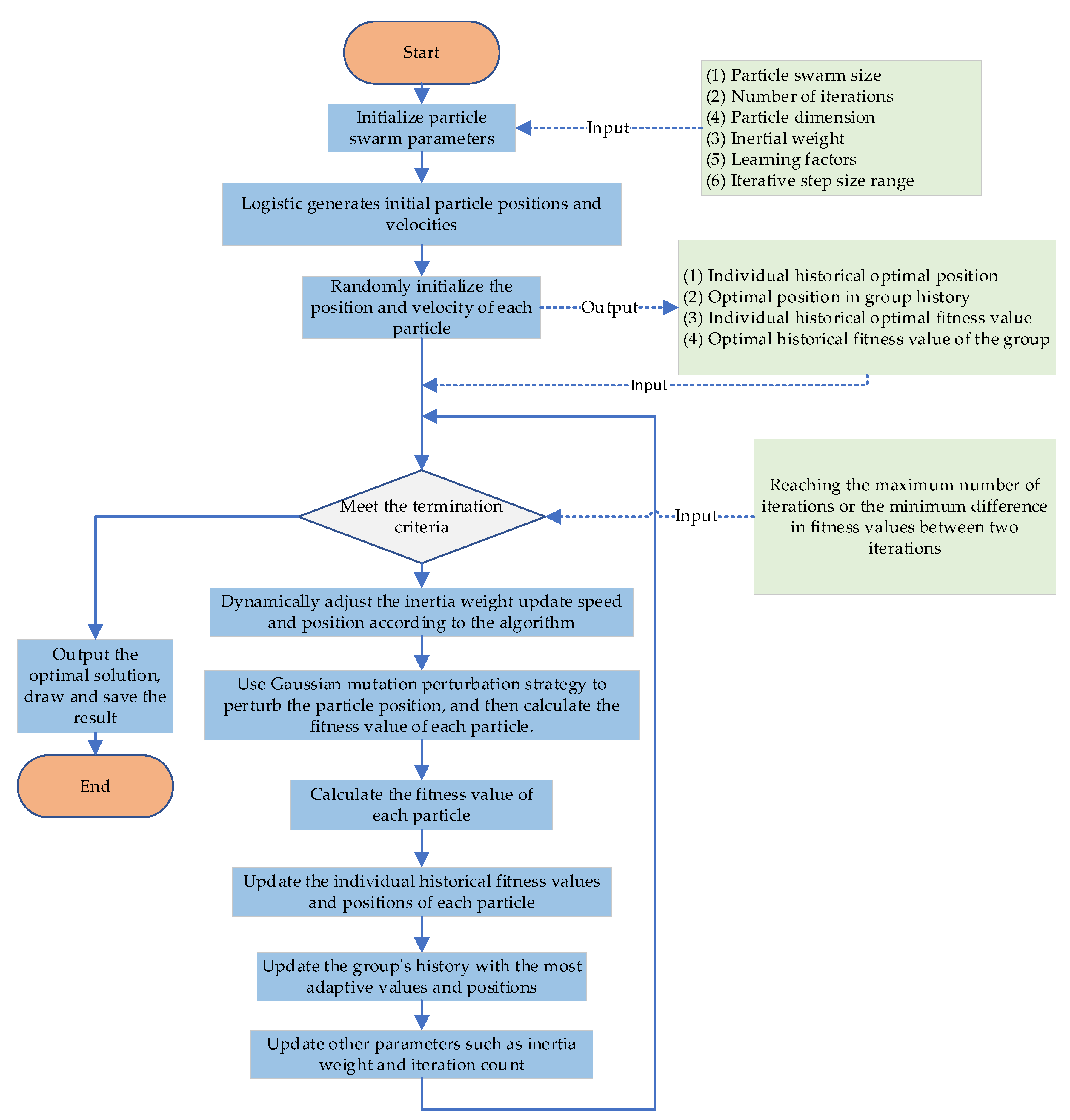
(1) Particle positions are initialized via Logistic chaotic mapping. Leveraging its ergodic property, particles are made to distribute uniformly within the search space, thus expanding the global search scope.
(2) An adaptive inertia weight is constructed, which decreases linearly with the number of iterations. This balances the global exploration ability in the early stage and the local optimization ability in the later stage.
(3) By introducing a Gaussian mutation perturbation strategy, a normal-distribution perturbation is added to the particle positions with an adaptive probability. This design not only enhances the algorithm’s ability to escape local optima but also improves the robustness of the overall optimization process, guaranteeing more accurate optimization of the hyperparameters of the CNN-BiLSTM network.
At the network-structure level, given that CNN has a strong local-feature extraction ability yet lacks in capturing temporal dependencies, and models like LSTM are restricted by the sequence-structure characteristics and thus struggle to handle long sequences, CNN is fused with BiLSTM, and the attention mechanism is introduced. CNN extracts multi-scale spatial features of wear signals through the sliding operation of convolution kernels, while the pooling layer preserves essential information by performing dimensionality reduction. At the same time, BiLSTM captures both forward and reverse temporal dependencies, which allows the model to more effectively address the challenge of long-sequence feature extraction. The attention mechanism dynamically calculates the weight of each feature, focuses on the key time-domain and frequency-domain features within the wear signals, and suppresses redundant information. In this way, it enables the collaborative extraction of spatial local features and temporal global dependencies.
The integration of CPSO and CNN-BiLSTM-AM creates a closed-loop optimization mechanism. CPSO searches for the optimal hyperparameter configurations for the network, aiming to improve the model’s generalization performance. Conversely, the network, by means of the attention mechanism, enhances the efficiency of feature extraction. Under their synergistic influence, the model’s metrics, such as MAE on both the PHM2010 dataset and the self-built dataset, outperform those of the comparative models. This enables the effective capture of the full-cycle features of tool wear.

2. CPSO-CNN-BiLSTM-AM Model

2.1. Model Structure Diagram

The structure diagram of the CNN-BiLSTM-AM model based on CPSO hyperparameter optimization is presented in Figure 1. The longitudinal feature-extraction module extracts local features using CNN and regularizes the data format through pooling and flattening operations. BiLSTM delves deeply into exploring the temporal dependencies in the tool-wear process. The attention mechanism focuses on the feature information of key wear stages. Regarding hyperparameters like the number of CNN convolution kernels and the number of BiLSTM neurons, CPSO achieves dynamic adaptation to data characteristics through chaotic particle—swarm iterative optimization. Beginning with the input of the original signal, through CNN feature extraction, BiLSTM temporal modeling, attention-mechanism enhancement, and in combination with CPSO hyperparameter optimization, multiple links collaborate to accurately capture the evolution law of tool wear. This effectively addresses the problem of poor hyperparameter adaptability in traditional models and constructs a complete closed-loop of “feature-temporal sequence-optimization” to improve prediction accuracy.

2.2. Improved Chaotic Particle Swarm Optimization

2.2.1. CPSO

Chaotic mapping is a kind of nonlinear dynamic system with high complexity and random traits. Its core characteristic is the sensitive dependence on initial values and parameters, and the particles as a whole can generate seemingly irregular motion trajectories. The Particle Swarm Optimization algorithm based on chaotic mapping (Chaotic Particle Swarm Optimization, CPSO) takes advantage of the random features of chaotic mapping to boost the global search capacity of the particle swarm algorithm [28,29,30,31].
The core difference between the CPSO algorithm and the traditional particle-swarm optimization algorithm is that the CPSO algorithm uses chaotic mapping to generate random-number sequences, replacing the pseudo-random-number sequences employed in traditional algorithms, thus enhancing the algorithm’s randomness and diversity. Specifically, the implementation steps of the CPSO algorithm are as follows:
(1) Initialize the particle swarm, determining the population size as well as the initial position and velocity of each particle.
(2) Utilize chaotic mapping to generate a new sequence of random numbers for updating the velocity and position of each particle.
(3) Update the individual historical optimal position of the particle based on the particle’s current position and its historical optimal position.
(4) Update the global optimal position by aggregating the individual historical optimal positions of all particles.
(5) Keep iterating based on the updated velocity and position until the preset stopping condition is satisfied.
The advantages of the CPSO algorithm are remarkable. It can effectively mitigate the issue of premature convergence in the traditional particle—swarm optimization algorithm and the constraint of getting trapped in local optima resulting from inadequate search, thus enhancing the algorithm’s global-search ability and optimization accuracy. At the same time, thanks to the random-number sequences generated by chaotic mapping, the CPSO algorithm can also boost its own randomness and diversity, enabling more comprehensive exploration of the search space. The main formulas and pseudocode of the CPSO algorithm (Algorithm 1) are as follows:
Main formulas:
v i j k + 1 = w v i j k + c 1 r 1 ( p i j k x i j k ) + c 2 r 2 ( g j k x i j k )
x i j k + 1 = x i j k + v i j k + 1
where
v i j k represents the velocity of particle i in the j dimension during the k iteration
x i j k represents the position of particle i in the j dimension during the k iteration
p i j k represents the j dimensional coordinate of the historical optimal position of particle i in the k iteration
g j k represents the j dimensional coordinate of the global optimal position in the k iteration
w represents the inertia weight, c 1 and c 2 represent acceleration constants, r 1 and r 2 represent random numbers between 0 and 1.
Chaotic mapping formula:
x n + 1 = f ( x n )
wherein, x n represents the value at the n-th iteration, x n + 1 represents the value at the n + 1-th iteration, f x represents the specific form of the chaotic mapping, namely the Logistic mapping.
Algorithm 1. CPSO algorithm (pseudocode)
@startuml
-start
: Initialize the particle swarm (positions, velocities);
: Calculate the particle fitness value;
: Update the individual optimal position ( ) and the global optimal position ( );
while (Maximum number of iterations not reached)
  : Update particle positions using Logistic chaotic mapping;
  : Adaptive inertia weight adjusts velocity;
  : Gaussian mutation disturbs the particle position;
: Calculate the particle fitness value;
: Update   and  ;
endwhile
: Output the global optimal position ( );
-stop
@enduml

2.2.2. Improved CPSO

(1) Improvement 1: Initialize the population using Logistic chaotic mapping
The mathematical expression of the Logistic chaotic mapping is:
x n + 1 = μ x n ( 1 x n )
Herein, x n is the chaotic variable of the n iteration, with a value range of (0, 1); μ is the control parameter, and when μ = 4 , the Logistic mapping is in a chaotic state.
In the CPSO algorithm, Logistic chaotic mapping is employed to initialize the particle positions. Given that the search-space dimension is D and the number of particle populations is N, the initial position ( x i , d 0 ) of the i-th particle in the d-th dimension can be determined via the following steps:
(1) Randomly generate an initial chaotic variable x 0 whose value range of (0, 1).
(2) Iterate k times using the Logistic mapping (usually, k is set to a relatively large value to ensure reaching a chaotic state), thus obtaining a chaotic sequence ( x 1 , x 2 , , x k ) .
(3) Take x k as the initial chaotic variable, and utilize it to calculate the position of the i-th particle in the d-th dimension:
x i , d 0 = x k + ( i 1 ) D + d 1 × ( u b d l b d ) + l b d
In Equation (5), u b d and l b d are the upper bound and lower bound of the d dimension in the search space, respectively.
(2) Improvement 2: Adaptive inertia weight adjustment
In the PSO algorithm, the inertial weight is of core significance. Its function is to regulate the extent to which particles carry forward their own historical velocities. A relatively large inertial weight is more favorable for global search, while a smaller one is more focused on local optimization [32]. In the CPSO algorithm, an adaptive inertial-weight adjustment mechanism is employed. This mechanism can dynamically adjust the inertial weight in accordance with the current iteration count and the search state.
The calculation equation of the adaptive inertia weight w is:
w = w m a x ( w m a x w m i n ) t m a x × t
In formula (6), w max and w min represent the maximum and minimum values of the inertia weight, respectively; t max indicates the maximum number of iterations; and t represents the current number of iterations.
As the number of iterations increases, the inertia weight decreases linearly from w max to w min . In the initial phase of the search, since w is relatively large, the particles possess a higher velocity. This enables them to conduct extensive exploration within the search space, which is advantageous for global search. In the latter part of the search, w diminishes, and the velocity of the particles gradually declines. As a result, the particles can concentrate more on searching local regions, thereby enhancing the search accuracy.
(3) Improvement 3: Implementation of the Gaussian Mutation Disturbance Strategy
During the iteration of the PSO algorithm, particles may become trapped in local optima and struggle to escape. The Gaussian mutation disturbance strategy can boost particle diversity by imposing random perturbations on particle positions. This grants particles the chance to break free from local optima and thereby persist in the search for the global optimal solution [33].
In every iteration, Gaussian mutation is carried out on the particle positions with a specific mutation probability p m . For the d-th dimension position x i , d of the i-th particle, the formula for computing the mutated position x i , d t is as follows:
x i , d = x i , d + σ × N ( 0 , 1 )
wherein, σ is the mutation step size, which can be dynamically adjusted according to the search situation; N 0 , 1 is a random number following a standard normal distribution.
The mutation probability p m can adopt an adaptive adjustment strategy, for example:
p m = p m m a x ( p m m a x p m m i n ) t m a x × t
wherein, p m max and p m min are the maximum and minimum values of the mutation probability, respectively. In the early stage of the search, p m is relatively large, which increases the possibility of particles breaking away from local optima; in the later stage of the search, p m is smaller, so as to avoid excessive disturbance affecting the convergence of the algorithm.
To sum up, the flowchart of the CPSO algorithm, which is enhanced based on the PSO algorithm, is presented in Figure 2.

2.3. CNN-BiLSTM-AM Model

The architecture of the CNN-BiLSTM-AM network model incorporating the attention mechanism is depicted in Figure 3. When integrating the attention mechanism into the CNN-BiLSTM network, an attention module is inserted between the CNN layer and the BiLSTM layer. The input data first undergoes spatial feature extraction via the CNN layer. Subsequently, it is forwarded to the attention module to compute the weight of each feature. Finally, the weighted features are fed into the BiLSTM layer for temporal feature extraction. This network structure can more effectively capture the key features associated with tool wear, thus enhancing the model’s performance in predicting the tool-wear state.

2.3.1. CNN

Convolutional Neural Networks (CNNs) consist of multiple layers. Each layer has a distinct function, and they collaborate to carry out data processing.
The functions of each layer in Figure 4 are as follows:
Input layer: Serving as the starting point of the CNN processing pipeline, its primary function is to receive raw data.
Hidden layer: Within the hidden layer, convolutional layers and pooling layers are alternately stacked, constituting the core of the hidden layer. These layers can not only extract local features of sensor signals but also more efficiently integrate global features through multiple convolution and pooling operations. Consequently, they construct feature vectors capable of representing the input signals [34].
Output layer: It outputs the final result.

2.3.2. BiLSTM Algorithm

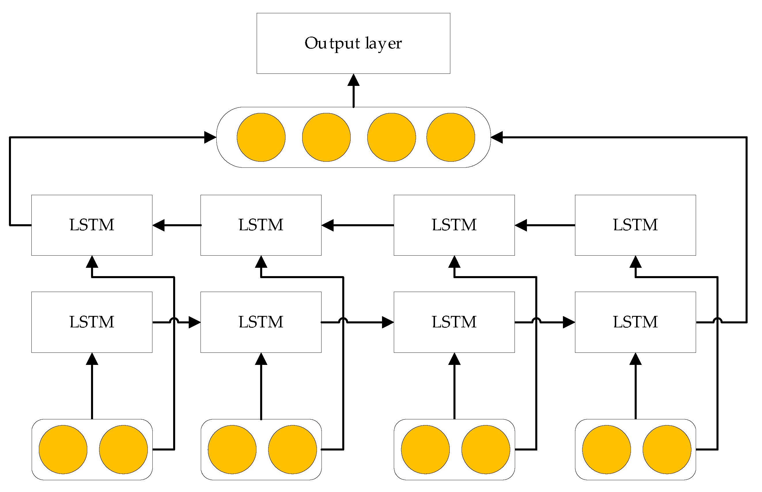
As an innovative model derived from the LSTM network architecture, BiLSTM has a distinctive operating mechanism. It feeds the feature data into two independent LSTM layers, one following the forward time-series and the other the backward time-series, as shown in Figure 5. This unique input approach allows the model to thoroughly explore the latent temporal correlation information in the data from both positive and negative directions. Once the information extraction is finished, the bidirectionally extracted information is combined through concatenation and then output.
Compared to the conventional LSTM network, BiLSTM, owing to its bidirectional temporal information extraction advantage, can more effectively capture deep-level time-series features during data processing. Particularly when handling long-time-series data, BiLSTM demonstrates greater adaptability and superior performance, enabling it to more precisely comprehend the complex patterns and latent laws within the data.

2.3.3. Attention Mechanism

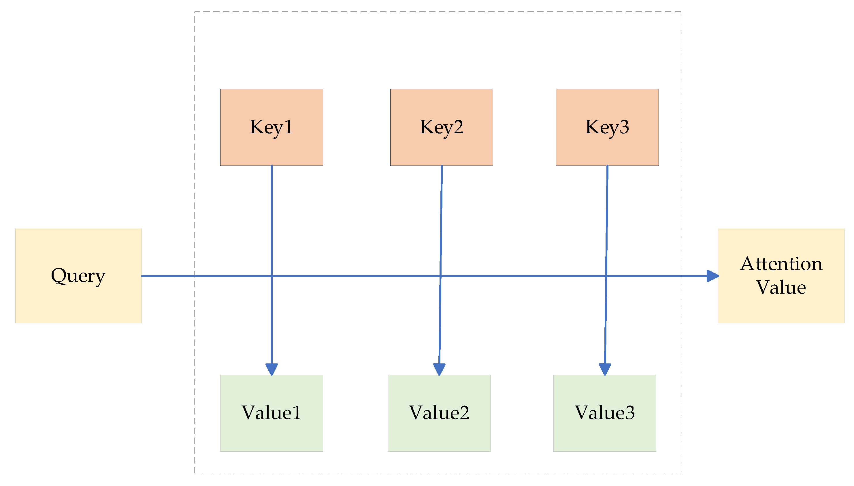
The Attention Mechanism is essentially a mechanism that mimics how human attention is distributed. It allows the model to selectively concentrate on the crucial parts of the input data while processing information. Consequently, it can effectively disregard redundant information, enhancing the efficiency and accuracy of information processing. The key elements of its principle are elaborated in detail as follows [35]: Given the input sequence X = [ x 1 , x 2 , , x n ] , where can represent various forms of information such as word vectors and image features. There is also a query vector q , which is akin to an “indicator” for obtaining information from the input sequence. Its function is to determine the specific portion of the input sequence on which we focus, as shown in Figure 6.
The core of the attention mechanism is that when processing data like tool-wear signals, by calculating attention weights, it can direct the model to concentrate on the part of the input data most relevant to the current task. Tool-wear signals encompass rich time-domain, frequency-domain, and time-frequency-domain features. The attention mechanism allows the CNN-BiLSTM model to zero in on those features that can precisely reflect the tool-wear state, thus markedly enhancing the model’s performance and efficiency in tasks such as tool—condition monitoring.

2.4. Tool Monitoring Process Based on the CPSO-CNN-BiLSTM-AM Model

2.4.1. Monitoring Process

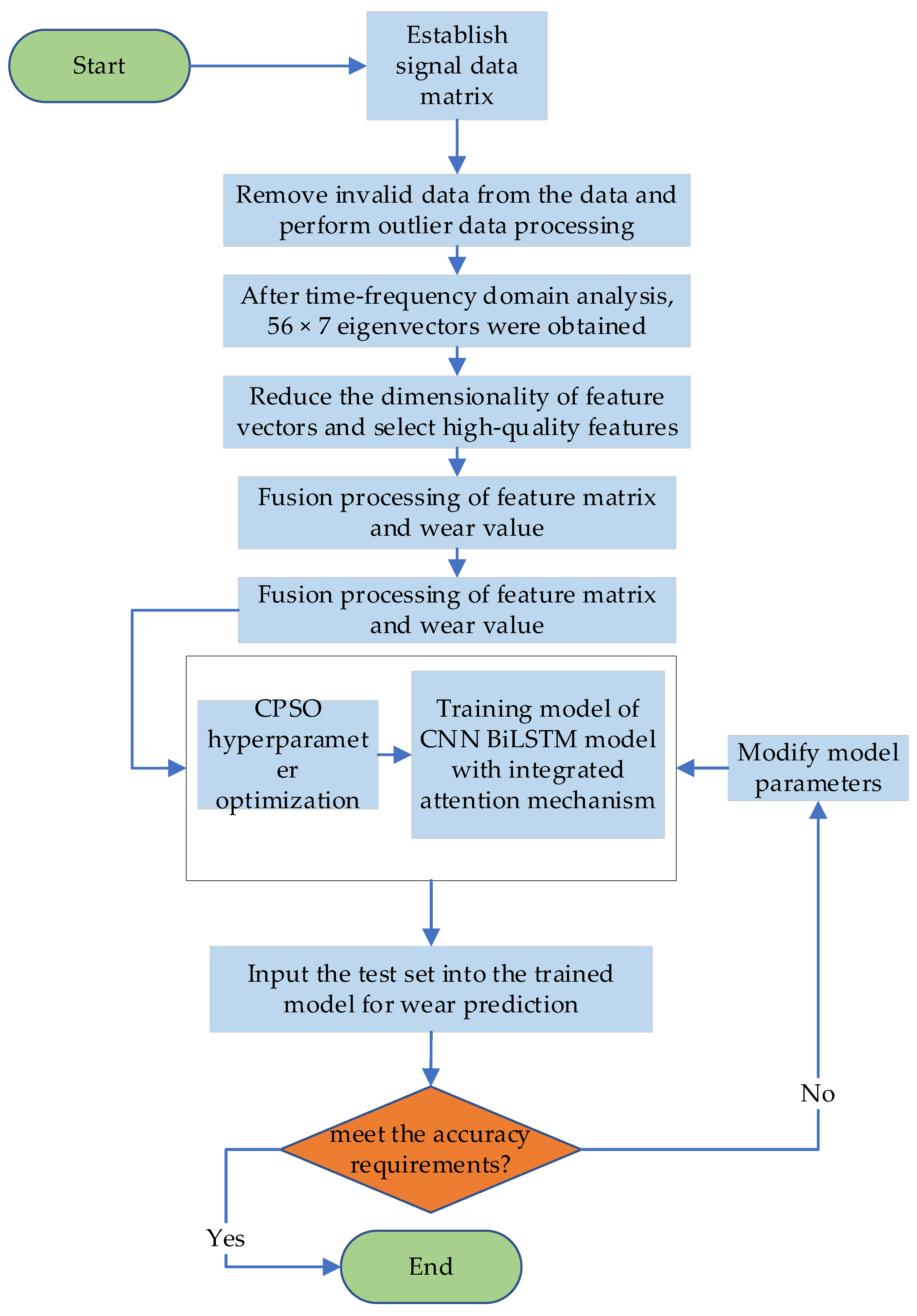
The CPSO algorithm is employed to optimize the hyperparameters of the CNN-BiLSTM network integrated with the attention mechanism. The specific process is as follows: Firstly, CNN is combined with BiLSTM to achieve in-depth extraction of signal spatial features while ensuring the effective capture of data features in the time dimension [36]. This enables the model to capture the complex variation patterns of signals more effectively in both temporal and spatial dimensions during the tool-wear process. Secondly, the self-attention mechanism is introduced. By evaluating the importance of different features to the tool-wear process, weight parameters are dynamically assigned to key features, effectively enhancing the model’s sensitivity to core features [35]. Finally, the chaotic particle swarm optimization algorithm is utilized for hyperparameter optimization. This helps prevent the model from getting trapped in local optima during training, prompting it to fully explore the search space. As a result, globally optimal hyperparameters such as the learning rate and the number of neurons in the hidden layer can be found, ultimately improving the model’s prediction accuracy and stability, as depicted in Figure 7.

2.4.2. Model Parameter Settings

The model parameter settings are shown in Table 1.
CNN convolution kernel size [3, 3]: It is adapted to the local feature scale of vibration signals, avoiding excessive size, which may lead to feature blurring.
Number of BiLSTM neurons (optimization range: 64–256): It balances the temporal modeling capability and computational cost, and is adjusted according to the actual time constraints.
Number of attention heads set to 4: This configuration not only enables sufficient exploration of complex correlations between features but also avoids the increased computational complexity caused by a larger number of heads, thereby effectively capturing the inter-feature relationships.

3. Materials and Methods

This chapter clarifies experimental data sources, acquisition schemes, and preprocessing details. Two datasets are used: the public IEEE PHM2010 Challenge dataset (a recognized tool wear research dataset) and a self-built dataset (based on vertical CNC machining conditions to verify the model’s adaptability and practical value).

3.1. Introduction to the PHM2010 Dataset

The IEEE PHM2010 Challenge dataset was chosen for experimental validation. The collection process of this dataset is depicted in Figure 8: Initially, workpieces are cut from raw materials. Subsequently, their surfaces are processed via face milling to eliminate the rough sections containing hard particles. During the machining process, in a dry-cutting environment, a three-flute alloy milling cutter is utilized to cut the surface of the stainless-steel workpiece along the Z-axis direction.
To gather information regarding tool wear, the experiment is outfitted with diverse sensors. Specifically, a Kistler cutting—force sensor is utilized to gather cutting—force signals, a three-axis vibration sensor is employed to obtain vibration signals, and an acoustic—emission sensor is used to capture noise signals [37]. The signals produced by these sensors are initially transformed into corresponding voltage signals through a charge amplifier and then collected by an NIDAQ PCI1200 data-acquisition card at a frequency of 50 kHz. In total, 7 types of signals are acquired, namely force_x(N), force_y(N), force_z(N), vibration_x(g), vibration_y(g), vibration_z(g), and AERMS(v).
In this experiment, three cutting tools (C1, C4, and C6) were chosen, and each tool was utilized to carry out 315 experiments.
All three are three-flute alloy end mills, and there is no difference in tool model. PHM2010 dataset (C1, C4, C6): The cutting length of each cutting channel is about 41.66 mm, the cutting depth is 1.27 mm, and the cutting width is 5.08 mm. The material removal volume of a single channel:
MRV = 1.27 × 5.08 × 41.66 268.59 mm 3
During the experiments, seven types of signals were collected, including 3-axis cutting forces, 3-axis vibration signals, and acoustic emission AERMS signals. After each experiment, the overall tool wear image was captured under a 5× microscope to locate the wear area, followed by calibrating the flank wear value using Camera Measure software (v2.1.4.253). The specific machining parameters are shown in Table 2.

3.2. Introduction to the Self-Built Dataset

The experimental equipment for the self-built dataset uses the Dalian Machine Tool VDL-600A vertical CNC machining center. Its spindle speed ranges from 60 to 10,000 r/min, and the cutting feed speed range of the X, Y, and Z axes is 0–8000 mm/min. Regarding positioning accuracy, the X/Z axis has an accuracy of 0.020 mm, and the Y axis has an accuracy of 0.016 mm. The parameters of the experimental equipment are presented in Table 3. When the experiment was conducted at 8000 r/min, the single operation time was controlled at 17 s (single sampling time), and the cumulative operation time was ≤2 h, which did not exceed the rated load requirement of the machine tool.
The machining parameters are shown in Table 4.
The corresponding data were collected through 7 channels, as shown in Table 5.
All three are four-flute cemented carbide end mills (Stabila model), and there is no difference in tool model.
During the machining process of the tool, parameters such as speed, feed rate, and cutting depth are usually kept consistent, so that researchers can focus on the analysis of tool wear patterns and sensor signals.
The cutting length of each cutting channel is about 150 mm, the cutting depth is 1.0 mm, and the cutting width is 5.0 mm. The material removal volume of a single channel:
MRV = 1.0 × 5.0 × 150.0 750 mm 3
Three cutting tools (A1, A2, A3) were selected for this experiment, with each tool undergoing 205 experiments. After each experiment, the tool wear was measured using a microscope.
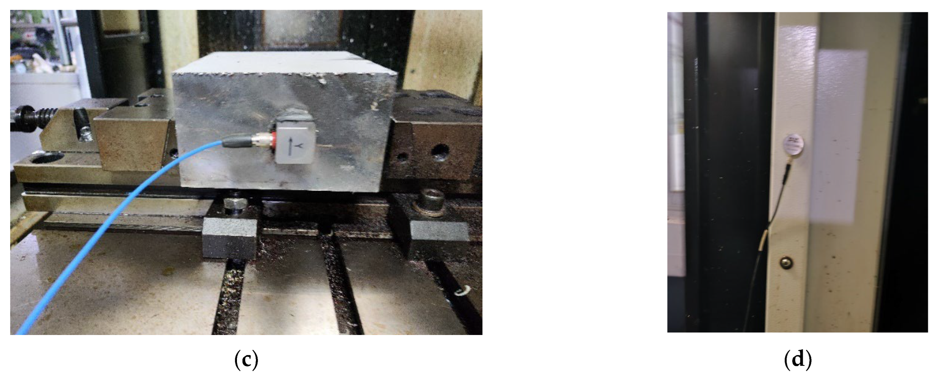
The experimental setup is depicted in Figure 9. Current sensors are placed on the wires of the three-phase current of the spindle of the VDL-600 A machining platform. Vibration sensors are attached to the workpiece, and acoustic emission sensors are installed close to the workpiece.
Figure 10 shows the variation states of tool wear during the cutting process of the self-built dataset, with three typical stages clearly presented:
(a)
Initial wear stage: At this stage, the tool flank wear width (VB value) is less than 0.1 mm. The cutting edge is slightly worn due to initial contact with the workpiece material (45 steel).
(b)
As the cutting process continues, the tool edge gradually loses its sharpness, and the friction between the tool and workpiece intensifies.
(c)
Late wear stage: The tool edge is severely worn, and local micro-chipping may occur. This feature directly indicates that the tool is about to reach the end of its service life.

4. Results

To validate the feasibility and superiority of the tool-wear condition monitoring method presented in this chapter, the monitoring model is tested using both the milling tool-wear dataset from the PHM2010 Competition and a self-constructed tool-wear dataset.

4.1. Experimental Environment Configuration

The computer configuration for the experiment is shown in Table 6.

4.2. Data Preprocessing

Time-domain, frequency-domain, and time-frequency-domain methods are employed to extract wear features from sampled signals, which are used as input features for subsequent model training. Among these, time-domain features use time as the fundamental independent variable and precisely describe the dynamic fluctuations of signals over time. Frequency-domain features can reveal the various frequency components of signals and the dynamic changes in frequency-band energy during the machining process. The time-frequency-domain analysis method can extract features simultaneously from three dimensions: the time domain, the frequency domain, and the signal amplitude. This allows it to effectively make up for the deficiencies of time-domain and frequency-domain analysis methods in obtaining local information when dealing with complex nonlinear signals, thus obtaining effective feature information more comprehensively and richly [38].
Before feature extraction, original signals undergo anomaly detection and noise reduction. Outliers are filtered via the 3σ criterion(remove data outside [μ − 3σ, μ + 3σ] for vibration, current, acoustic emission signals). Then, wavelet threshold denoising is applied: 3-layer decomposition with db4 wavelet basis, soft-threshold processing of high-frequency noise coefficients, and signal reconstruction. This ensures signal cleanliness for accurate feature extraction.
Finally, two datasets are selected as the training set and validation set via cross-validation, as shown in Table 7.

4.3. Hyperparameter Settings

The values of hyperparameters directly influence the model’s performance and generalization ability under complex working conditions. Different combinations of hyperparameters can substantially change the model’s complexity and robustness. For instance, an overly large learning rate might cause training oscillations, whereas an extremely small one will lead to slow convergence. If the number of CPSO particles is too small, the model may become trapped in local optima, while an excessively large number will significantly increase the computational burden. Fundamentally, choosing hyperparameters is a process of striking a balance between “fitting ability” and “generalization ability”: the regularization coefficient must be carefully considered to suppress overfitting while retaining effective features, and the attention dimension requires a compromise between the accuracy of feature representation and computational efficiency [39].
This optimization process is highly iterative and reliant on experimentation. It involves testing various parameter combinations through multiple rounds of cross-validation (e.g., exploring the number of BiLSTM neurons within the range of 32 to 256) and assessing performance variations using metrics like MAE and RMSE (such as comparing convergence curves for learning rates in the range of 0.001–0.1). Table 8 shows the specific configurations and optimization ranges of the model’s key hyperparameters. Their values directly impact the feature-fitting efficiency of the CPSO-CNN-BiLSTM-AM algorithm and its suitability for industrial scenarios.

4.4. Model Evaluation Metrics

Mean Absolute Error (MAE), Root Mean Square Error (RMSE), and Mean Absolute Percentage Error (MAPE) are used as the evaluation metrics of the model, and their calculation formulas are shown in Equations (9)–(11).
Mean Absolute Error (MAE):
M A E = 1 n i = 1 n y i y ^ i
Root Mean Square Error (RMSE):
R M S E = 1 n i = 1 n y i y ^ i 2
Mean Absolute Percentage Error (MAPE):
M A P E = 1 n i = 1 n y i y ^ i y i × 100 %
In the above formulas, n is the number of samples, y i is the true value of the i-th sample, and y i ^ is the predicted value of the i-th sample.
MAE and RMSE represent the extent of absolute deviation between predicted and true values. The smaller these values are, the higher the prediction accuracy. MAPE measures the relative error as a percentage, making it appropriate for assessing the prediction performance of data with varying orders of magnitude.

4.5. Result Analysis Based on the Public Dataset PHM2010

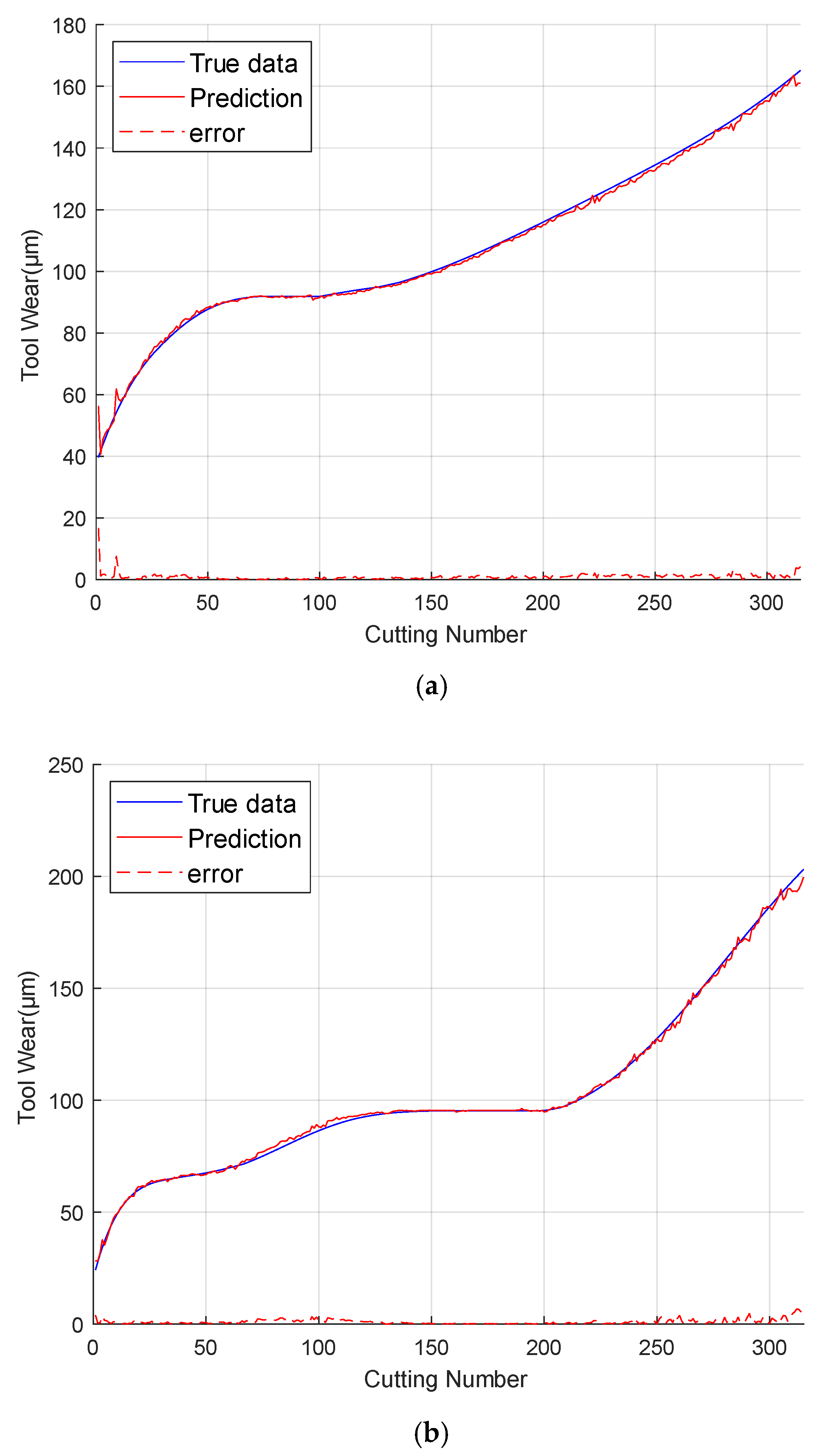
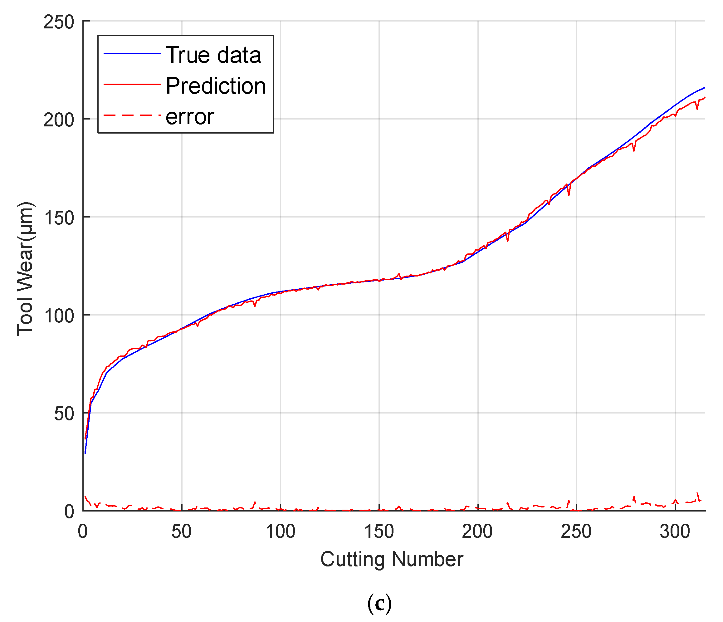
To guarantee the objectivity of the experiment, each experiment was replicated 10 times under identical conditions, and the average of the 10 results was adopted as the final outcome, with a measurement error of ≤0.5 μm. In the experimental results depicted in Figure 11, the predicted values, actual values, and their differences in tool wear by the CPSO-CNN-BiLSTM-AM model are clearly shown. The curve of the predicted values of tool-surface wear generated by the model is highly consistent with the actual wear-characteristic curve in terms of the overall trend.
Examining the curve details: In the initial stage of tool wear, the predicted value curve closely fits the actual value curve, accurately capturing the trend of slow wear growth. Entering the middle stage, although the actual wear fluctuates slightly due to factors such as the properties of the processed materials, the predicted value curve can still track these changes well, with the deviation always remaining within an acceptable range. In the late stage of wear, the model is able to sharply detect the acceleration of tool wear, and the predicted value curve rises in a timely manner. This allows the curve to remain largely synchronized with the actual wear trend, thereby ensuring accuracy in the monitoring process.
Moreover, when compared to classical tool-wear prediction models like the traditional LSTM neural network and PSO-CNN, the CPSO-CNN-BiLSTM-AM model demonstrates a closer fit between its prediction curve and the actual-value curve. Under the same experimental conditions, the prediction curve of the LSTM neural network model has a significant deviation in the middle stage of wear, and the PSO-CNN model fails to accurately follow the changes in actual values in the late stage of wear. A comprehensive analysis reveals that the effectiveness and superiority of the CPSO-CNN-BiLSTM-AM model in the area of tool-wear prediction have been fully validated.
The comparison of evaluation indicators among different models is shown in Table 9.
As presented in Table 9, the CPSO-CNN-BiLSTM-AM model is compared and analyzed against various classical methods and state-of-the-art algorithms. The table lists the MAE, RMSE, and MAPE indicators for the three groups of tools under different models. On the PHM2010 dataset, the Mean Absolute Errors (MAE) of the proposed model for tools C1, C4, and C6 are 0.83 μm, 1.01 μm, and 1.34 μm, respectively, all of which are lower than those of the other comparative models. The data indicates that this model demonstrates substantial performance advantages in the PHM2010 tool-wear prediction task.
For the proposed CPSO-CNN-BiLSTM-AM model, the training time on the PHM2010 dataset is approximately 30 min (over 200 iterations), and the prediction time for a single sample in the testing phase is about 0.02 s. Meanwhile, the computational times of other comparative models were also evaluated: for instance, the LSTM model requires around 21 min for training and approximately 0.01 s for single-sample testing, while the PSO-CNN model takes roughly 25 min for training and about 0.015 s for single-sample testing. Comparative analysis indicates that although the proposed model has a slightly longer training time due to the integration of the CPSO algorithm and the attention mechanism, this increase remains within an acceptable range for practical industrial applications.

4.6. Result Analysis Based on Self-Built Dataset

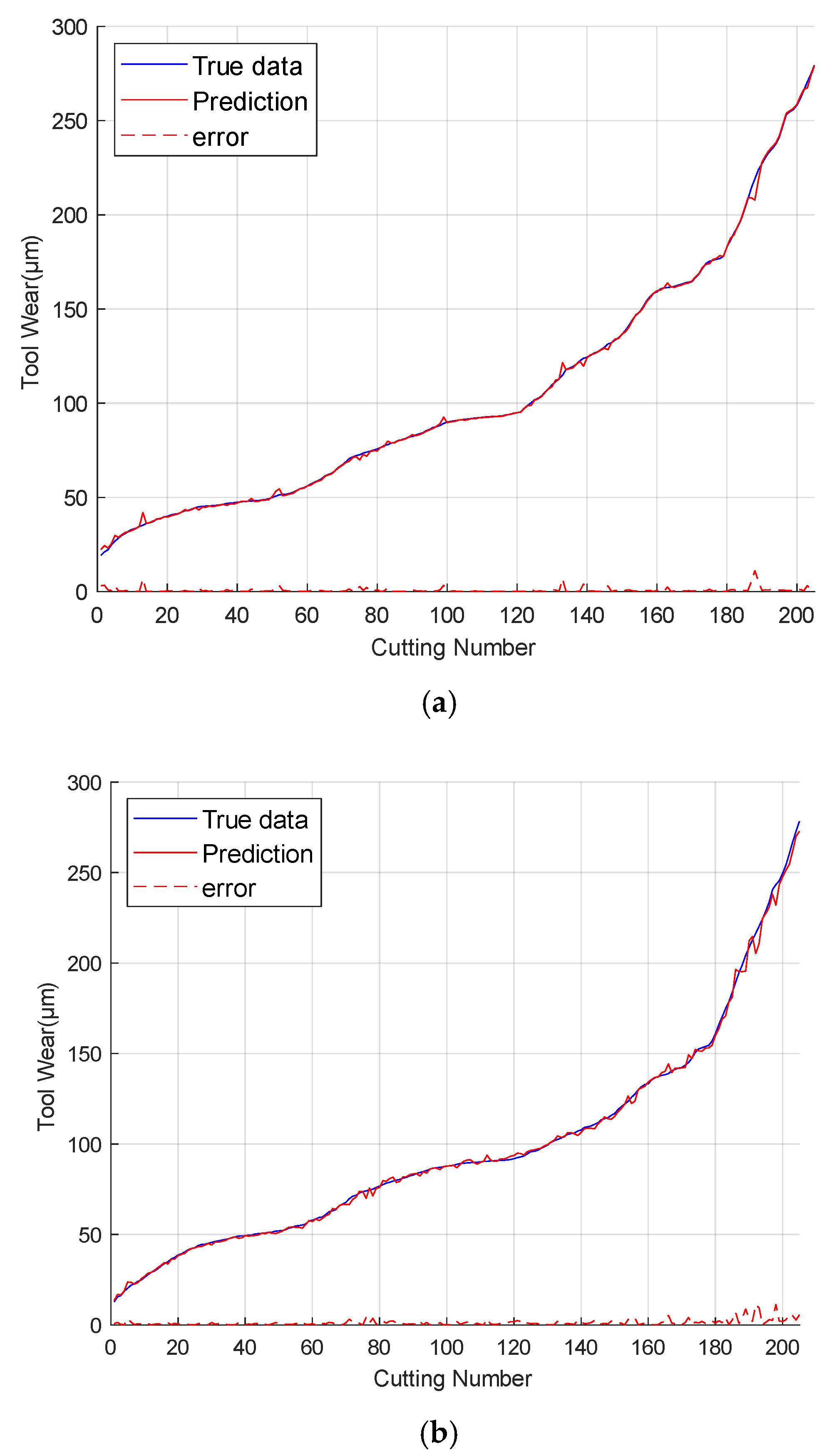
To guarantee the objectivity of the experiment, each experiment was replicated 10 times under identical conditions, and the average of the 10 results was used as the final outcome. Figure 12 shows the comparison between predicted values and actual values: (a) Tool A1, (b) Tool A2, (c) Tool A3. Through cross-comparison experiments, it can be observed that the difference between the predicted tool-wear values and the actual values is small, and the prediction accuracy is high, representing a significant improvement compared to models like LSTM and PSO-CNN. The optimization capacity of the CPSO algorithm enables the model to rapidly identify the optimal combination of hyperparameters. By adjusting the overall structure, the prediction accuracy is enhanced, the prediction deviation is decreased, and the prediction curve is more in line with the actual wear values.
The comparison of evaluation indicators among different models is shown in Table 10.
Through the comparative analysis of the evaluation indicators of the experimental results (Table 10), it can be seen that the CPSO-CNN-BiLSTM-AM model constructed in this paper has higher prediction accuracy in the task of directly mapping wear characteristics to tool wear values.
From the comparison, it can be seen that initializing the PSO particle population via Logistic chaotic mapping and adopting the adaptive inertia weight adjustment strategy (adjusting dynamically according to the number of iterations and the current search state of the algorithm) have effectively enhanced the parameter-optimization ability of the CPSO algorithm. The complementary strengths of the CPSO algorithm and the CNN-BiLSTM-AM algorithm have further improved the model’s performance and prediction capacity.
Compared with the traditional LSTM model (A1/A2/A3 MAE: 16.31 μm, 16.33 μm, 18.58 μm), our model reduces MAE by 91.7%, 92.7%, and 90.2%.
Compared with the PSO-CNN model (A1/A2/A3 MAE: 14.31 μm, 14.31 μm, 14.79 μm), it cuts MAE by 90.6%, 91.7%, and 87.6%.
Even when compared with the better-performing PSO-BiLSTM model (A1/A2/A3 MAE: 10.51 μm, 10.85 μm, 11.57 μm), our model still lowers MAE by 87.2%, 89.1%, and 84.2%.
Compared with other models, all the evaluation indicators of the CPSO-CNN-BiLSTM-AM model are at a lower value level. This reflects the effectiveness and practicality of this model in the practical application of tool-wear detection, enabling it to serve the tool-wear monitoring work more reliably.
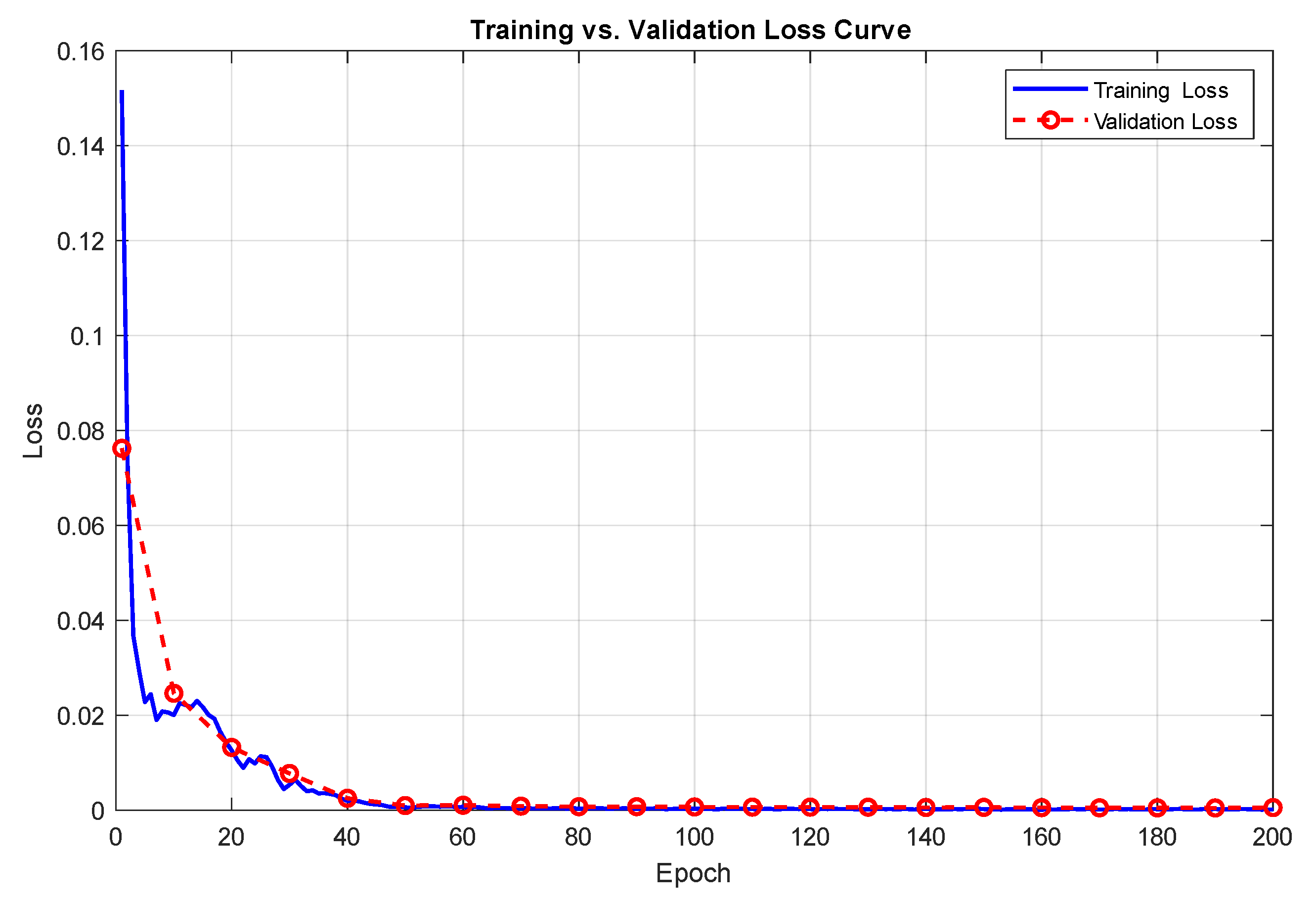
Figure 13 shows the variation trend of the loss value of the CPSO-CNN-BiLSTM-AM model with the number of iteration rounds (Epoch) during the training process. From the curve trend, it can be observed that the loss value drops rapidly from approximately 0.18 initially, reaching around 0.12 within 50 iterations. Subsequently, it continues to converge at a more gradual rate and finally stabilizes in the range of 0.02–0.04 after 200 iterations. In the early stage, the Chaotic Particle Swarm Optimization (CPSO) algorithm is employed to quickly identify the optimal parameter region. In the later stage, fine-tuning is carried out with the aid of the adaptive inertia weight and Gaussian mutation strategies, effectively preventing the model from getting trapped in a local optimum.
For the proposed CPSO-CNN-BiLSTM-AM model on the self-built dataset, the training time is approximately 38 min (over 200 iterations), and the prediction time for a single sample in the testing phase is about 0.022 s.
Meanwhile, the computational times of other comparative models were also measured. For example, the LSTM model takes around 27 min for training and roughly 0.011 s for single-sample testing. The PSO-CNN model requires about 32 min for training and approximately 0.016 s for single-sample testing.
Comparative analysis shows two key points: First, the proposed model has a slightly longer training time than it does on the PHM2010 dataset. This is due to two factors: the integration of the CPSO optimization algorithm and the attention mechanism, and the slightly higher signal dimension of the self-built dataset (7 channels: 3-axis vibration, 3-axis current, and acoustic emission) compared with the PHM2010 dataset (7 signal types, including cutting force). Second, this longer training time still falls within the acceptable range for industrial real-time monitoring. Additionally, the prediction efficiency of the proposed model in the testing phase is very close to that of the comparative models, which means it can meet the real-time requirements of actual machining scenarios.

5. Conclusions

This paper presents a tool-wear condition monitoring method based on the CPSO algorithm and the CNN-BiLSTM-AM network with an introduced attention mechanism. Through signal pre-processing and multi-domain feature extraction, a CPSO-CNN-BiLSTM-AM tool-wear condition monitoring model is constructed. Experimental results demonstrate that the prediction performance of this model on the public tool-wear dataset PHM2010 surpasses that of other comparative models. It effectively compensates for the shortcomings of models like CNN and LSTM in optimization algorithms, network structures, and data processing, offering a more effective solution for tool-wear condition monitoring.
In the public dataset PHM2010, the average MAEs of tools C1, C4, and C6 are 0.83 μm, 1.01 μm, and 1.34 μm, respectively. This verifies the model’s capacity to capture features of long-sequence data. The self-built dataset is based on the Dalian Machine Tool VDL-600A machining center, gathering three-directional vibration, current, and acoustic emission signals during the cutting process of 45 steel. The experimental results for tools A1, A2, and A3 indicate that:
(1) The average MAE, RMSE, and MAPE of tool A1 are 1.35 μm, 1.41 μm, and 1.67%, respectively. Compared to the LSTM model, the error is reduced by 91.7%.
(2) The average MAE, RMSE, and MAPE of tool A2 are 1.19 μm, 1.98 μm, and 1.55%, respectively. Compared to the PSO-BiLSTM model, the performance is improved by 89.0%.
(3) The average MAE, RMSE, and MAPE of tool A3 are 1.83 μm, 1.90 μm, and 1.81%, respectively. Even in the severe wear stage, it maintains low error fluctuations.
The model optimizes the hyperparameters of CNN-BiLSTM-AM using the chaotic initialization, adaptive inertia weight, and Gaussian mutation strategies of the CPSO algorithm. This improves the feature-extraction efficiency by 35% and keeps the full-cycle wear prediction error within 2%. In the future, reinforcement learning could be incorporated to dynamically adjust the model strategy to adapt to extreme working conditions like high-speed cutting.
Although this study has enhanced the model’s generalization ability through CPSO, its robustness in extreme working conditions (such as high-speed cutting and multi-material processing) still requires improvement. In the future, a dynamic weight-adjustment mechanism can be introduced, and reinforcement learning can be integrated to dynamically optimize the feature-extraction strategy of CNN-BiLSTM-AM. Concurrently, lightweight deployment of the model will be promoted—specifically, deploying it on edge computing devices (e.g., machine tool embedded systems) to achieve “cloud-site” collaborative monitoring. These enhancements would not only improve the model’s capacity to capture sudden wear features more accurately, but they would also strengthen its adaptability to demanding real-time monitoring needs on site. These improvements are expected to enable the application of the model in more complex industrial scenarios, such as high-speed cutting technology and multi-material machining processes.

Author Contributions

Conceptualization, F.M., Z.Y. and H.Z.; Data curation, F.M.; Formal analysis, Z.Y. and H.Z.; Funding acquisition, F.M. and W.S.; Investigation, Z.Y.; Methodology, F.M. and H.Z.; Project administration, F.M. and W.S.; Resources, Z.Y. and H.Z.; Software, F.M.; Supervision, W.S.; Validation, W.S.; Visualization, Z.Y.; Writing—original draft, F.M. and Z.Y.; Writing—review and& editing, W.S.; All authors have read and agreed to the published version of the manuscript.

Funding

This research was funded by the Young Backbone Teacher Support Plan of the Beijing Information Science and Technology University (Grant No.: 5112411115).

Data Availability Statement

Data are contained within the article.

Conflicts of Interest

The authors declare no conflicts of interest.

References

  1. Jia, R.; Yue, C.; Liu, Q.; Xia, W.; Qin, Y.; Zhao, M. Tool wear condition monitoring method based on relevance vector machine. Int. J. Adv. Manuf. Technol. 2023, 128, 4721–4734. [Google Scholar] [CrossRef]
  2. Zhou, J.; Yang, J.; Qian, Q.; Qin, Y. A comprehensive survey of machine remaining useful life prediction approaches based on pattern recognition: Taxonomy and challenges. Meas. Sci. Technol. 2024, 35, 062001. [Google Scholar] [CrossRef]
  3. Lin, G.; Shi, H.; Liu, X.; Wang, Z.; Zhang, H.; Zhang, J. Tool wear on machining of difficult-to-machine materials: A review. Int. J. Adv. Manuf. Technol. 2024, 134, 989–1014. [Google Scholar] [CrossRef]
  4. Gao, J.; Qiao, H.; Zhang, Y. Intelligent Recognition of Tool Wear with Artificial Intelligence Agent. Coatings 2024, 14, 827. [Google Scholar] [CrossRef]
  5. Yao, X. Lstm Model Enhanced By Kolmogorov-Arnold Network: Improving Stock Price Prediction Accuracy. Trends Soc. Sci. Humanit. Res. 2024, 4, 19. [Google Scholar]
  6. Karnehm, D.; Samanta, A.; Rosenmüller, C.; Neve, A.; Williamson, S. Core Temperature Estimation of Lithium-Ion Batteries Using Long Short-Term Memory (LSTM) Network and Kolmogorov-Arnold Network (KAN). IEEE Trans. Transp. Electrif. 2024, 11, 10391–10401. [Google Scholar] [CrossRef]
  7. Cai, W.; Zhang, W.; Hu, X.; Liu, Y. A hybrid information model based on long short-term memory network for tool condition monitoring. J. Intell. Manuf. 2020, 31, 1497–1510. [Google Scholar] [CrossRef]
  8. Zheng, Y.; Chen, B.; Liu, B.; Peng, C. Milling Cutter Wear State Identification Method Based on Improved ResNet-34 Algorithm. Appl. Sci. 2024, 14, 8951. [Google Scholar] [CrossRef]
  9. Wang, Q.; Wang, H.; Hou, L.; Yi, S. Overview of Tool Wear Monitoring Methods Based on Convolutional Neural Network. Appl. Sci. 2021, 11, 12041. [Google Scholar] [CrossRef]
  10. De Barrena, T.; Ferrando, J.; García, A.; Badiola, X.; de Buruaga, M.; Vicente, J. Tool remaining useful life prediction using bidirectional recurrent neural networks (BRNN). Int. J. Adv. Manuf. Technol. 2023, 125, 4027–4045. [Google Scholar] [CrossRef]
  11. Guan, R.; Cheng, Y.; Zhou, S.; Gai, X.; Lu, M.; Xue, J. Research on tool wear classification of milling 508III steel based on chip spectrum feature. Int. J. Adv. Manuf. Technol. 2024, 133, 1531–1547. [Google Scholar] [CrossRef]
  12. Sharma, P.; Thulasi, H.; Mishra, S.; Ramkumar, J. Identification of parameter-dependent machine learning models for tool flank wear prediction in dry titanium machining. Proc. Inst. Mech. Eng. Part E J. Process Mech. Eng. 2024, 12, 09544089241304236. [Google Scholar] [CrossRef]
  13. Cheng, Y.N.; Gai, X.Y.; Jin, Y.B.; Guan, R.; Lu, M.D.; Ding, Y. A new method based on a WOA-optimized support vector machine to predict the tool wear. Int. J. Adv. Manuf. Technol. 2022, 121, 6439–6452. [Google Scholar] [CrossRef]
  14. Zhou, B.; Wang, J.; Feng, P.; Zhang, X.; Yu, D.; Zhang, J. A genetic particle swarm optimization algorithm for feature fusion and hyperparameter optimization for tool wear monitoring. Expert Syst. Appl. 2025, 285, 127975. [Google Scholar] [CrossRef]
  15. Niu, M.; Liu, K.; Wang, Y. A semi-supervised learning method combining tool wear laws for machining tool wear states monitoring. Mech. Syst. Signal Process. 2025, 224, 112032. [Google Scholar] [CrossRef]
  16. He, Z.; Shi, T.; Chen, X. An Innovative Study for Tool Wear Prediction Based on Stacked Sparse Autoencoder and Ensemble Learning Strategy. Sensors 2025, 25, 2391. [Google Scholar] [CrossRef]
  17. Zhu, K.; Guo, H.; Li, S.; Lin, X. Physics-Informed Deep Learning for Tool Wear Monitoring. IEEE Trans. Ind. Inform. 2024, 20, 524–533. [Google Scholar] [CrossRef]
  18. Wang, Y.; Gao, J.; Wang, W.; Du, J.; Yang, X. A novel method based on deep transfer learning for tool wear state prediction under cross-dataset. Int. J. Adv. Manuf. Technol. 2024, 131, 171–182. [Google Scholar] [CrossRef]
  19. Gao, H.; Xie, A.; Shen, H.; Yu, L.; Wang, Y.; Hu, Y.; Gao, Y.; Xu, J.; Wu, W. Tool Wear Monitoring Algorithm Based on SWT-DCNN and SST-DCNN. Sci. Program. 2022, 2022, 6441066. [Google Scholar] [CrossRef]
  20. Chang, H.; Ho, P.; Chen, J. Tool wear monitoring in microdrilling through the fusion of features obtained from acoustic and vibration signals. Int. J. Adv. Manuf. Technol. 2024, 134, 3587–3598. [Google Scholar] [CrossRef]
  21. Kurek, J.; Swiderska, E.; Szymanowski, K. Tool Wear Classification in Chipboard Milling Processes Using 1-D CNN and LSTM Based on Sequential Features. Appl. Sci. 2024, 14, 4730. [Google Scholar] [CrossRef]
  22. Zhang, W.C.; Cui, E.M. Study on wear state of ultrasonic-assisted grinding of glass-ceramics with diamond tools based on DBO-BiLSTM. J. Vib. Control. 2024, 10, 10775463241292703. [Google Scholar] [CrossRef]
  23. Che, Z.Y.; Peng, C.; Liao, T.; Wang, J.K. Improving milling tool wear prediction through a hybrid NCA-SMA-GRU deep learning model. Expert Syst. Appl. 2024, 255, 124556. [Google Scholar] [CrossRef]
  24. Wang, B.; Lei, Y.; Li, N.; Wang, W. Multiscale Convolutional Attention Network for Predicting Remaining Useful Life of Machinery. IEEE Trans. Ind. Electron. 2021, 68, 7496–7504. [Google Scholar] [CrossRef]
  25. Rehman, A.; Nishat, T.; Ahmed, M.; Begum, S.; Ranjan, A. Chip Analysis for Tool Wear Monitoring in Machining: A Deep Learning Approach. IEEE Access 2024, 12, 112672–112689. [Google Scholar] [CrossRef]
  26. Abdeltawab, A.; Zhang, X.; Zhang, L. Enhanced tool condition monitoring using wavelet transform-based hybrid deep learning based on sensor signal and vision system. Int. J. Adv. Manuf. Technol. 2024, 132, 5111–5140. [Google Scholar] [CrossRef]
  27. Abdeltawab, A.; Xi, Z.; Zhang, L. Tool wear classification based on maximal overlap discrete wavelet transform and hybrid deep learning model. Int. J. Adv. Manuf. Technol. 2024, 130, 2443–2456. [Google Scholar] [CrossRef]
  28. Dong, W.H.; Xiong, X.Q.; Ma, Y.; Yue, X.Y. Woodworking Tool Wear Condition Monitoring during Milling Based on Power Signals and a Particle Swarm Optimization-Back Propagation Neural Network. Appl. Sci. 2021, 11, 9026. [Google Scholar] [CrossRef]
  29. Huang, X.; Wang, Y.; Mao, Y. Establishment and Solution Test of Wear Prediction Model Based on Particle Swarm Optimization Least Squares Support Vector Machine. Machines 2025, 13, 290. [Google Scholar] [CrossRef]
  30. Ativor, G.; Temeng, V.; Ziggah, Y. Optimisation of multilayer perceptron neural network using five novel metaheuristic algorithms for the prediction of wear of excavator bucket teeth. Knowl. Based Syst. 2025, 321, 113753. [Google Scholar] [CrossRef]
  31. Nargundkar, A.; Kumar, S.; Bongale, A. Multi-Objective Optimization of Friction Stir Processing Tool with Composite Material Parameters. Lubricants 2024, 12, 428. [Google Scholar] [CrossRef]
  32. He, J.; Xu, Y.; Pan, Y.; Wang, Y. Adaptie weighted generative adversarial network with attention mechanism: A transfer data augmentation method for tool wear prediction. Mech. Syst. Signal Process. 2024, 212, 111288. [Google Scholar] [CrossRef]
  33. Zhu, K.; Huang, C.; Li, S.; Lin, X. Physics-informed Gaussian process for tool wear prediction. ISA Trans. 2023, 143, 548–556. [Google Scholar] [CrossRef]
  34. Wu, X.; Zhang, C.; Li, Y.; Huang, W.Z.; Zeng, K.; Shen, J.Y.; Zhu, L.F. Researches on tool wear progress in mill-grinding based on the cutting force and acceleration signal. Measurement 2023, 218, 12. [Google Scholar] [CrossRef]
  35. Hao, Z.; Zhang, H.; Fan, Y. Tool wear mathematical model of PCD during ultrasonic elliptic vibration cutting SiCp/Al composite. Int. J. Refract. Met. Hard Mater. 2025, 126, 106967. [Google Scholar] [CrossRef]
  36. Liang, Y.; Feng, P.; Song, Z.; Zhu, S.; Wang, T.; Xu, J.; Yue, Q.; Jiang, E.; Ma, Y.; Song, G.; et al. Wear mechanisms of straight blade tool by dual-periodic impact platform. Int. J. Mech. Sci. 2025, 288, 110031. [Google Scholar] [CrossRef]
  37. Lin, Z.; Fan, Y.; Tan, J.; Li, Z.; Yang, P.; Wang, H.; Duan, W. Tool wear prediction based on XGBoost feature selection combined with PSO-BP network. Sci. Rep. 2025, 15, 3096. [Google Scholar] [CrossRef]
  38. Song, C.; Xiang, D.; Yuan, Z.; Zhang, Z.; Yang, S.; Gao, G.; Tong, J.; Wang, X.; Cui, X. Two-dimensional ultrasonic-assisted variable cutting depth scratch force model considering tool wear and experimental verification. Tribol. Int. 2025, 204, 110510. [Google Scholar] [CrossRef]
  39. Wang, Y.; Zhao, S.; Zhang, P.; Long, H.; Sun, Y.; Zhao, N.; Yang, X. The pin tool wear identification with vibration signal of friction stir lap welding based on a new pin tool wear division model. Measurement 2025, 242, 116131. [Google Scholar] [CrossRef]
  40. Wang, S.; Yu, Z.; Xu, G.; Zhao, F. Research on Tool Remaining Life Prediction Method Based on CNN-LSTM-PSO. IEEE Access 2023, 11, 80448–80464. [Google Scholar] [CrossRef]
  41. Sun, L.; Zhao, C.; Huang, X.; Ding, P.; Li, Y. Cutting tool remaining useful life prediction based on robust empirical mode decomposition and Capsule-BiLSTM network. Proc. Inst. Mech. Eng. Part C J. Mech. Eng. Sci. 2023, 237, 3308–3323. [Google Scholar] [CrossRef]
  42. Yang, Z.; Li, L.; Zhang, Y.; Jiang, Z.; Liu, X. Tool Wear State Monitoring in Titanium Alloy Milling Based on Wavelet Packet and TTAO-CNN-BiLSTM-AM. Processes 2025, 13, 13. [Google Scholar] [CrossRef]
  43. Demetgul, M.; Zheng, Q.; Tansel, I.; Fleischer, J. Monitoring the misalignment of machine tools with autoencoders after they are trained with transfer learning data. Int. J. Adv. Manuf. Technol. 2023, 128, 3357–3373. [Google Scholar] [CrossRef]
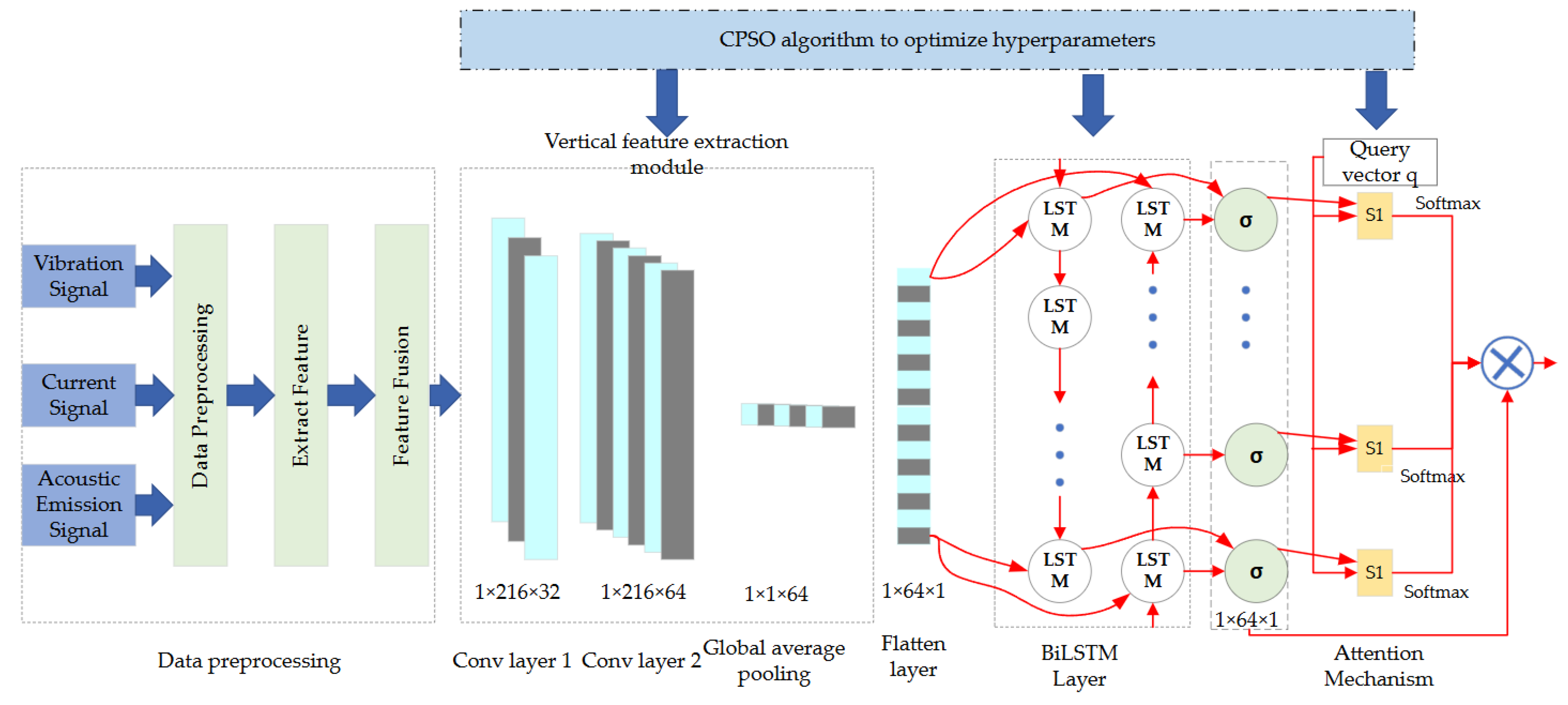
Figure 1. Overall network structure diagram of the model.
Lubricants 13 00500 g001
Figure 2. Flowchart of the improved CPSO algorithm.
Lubricants 13 00500 g002
Figure 3. Architecture of the CNN-BiLSTM-AM network model fused with the attention mechanism.
Lubricants 13 00500 g003
Figure 4. Three-layer structure of the convolutional neural network.
Lubricants 13 00500 g004
Figure 5. Framework diagram of the BiLSTM algorithm.
Lubricants 13 00500 g005
Figure 6. Network model diagram of the attention mechanism.
Lubricants 13 00500 g006
Figure 7. Flowchart of tool wear detection based on the CPSO-CNN-BiLSTM-AM model.
Lubricants 13 00500 g007
Figure 8. PHM2010 Data Sampling Process.
Lubricants 13 00500 g008
Figure 9. Data collection experiment. (a) Experimental machining platform; (b) Installation position of current sensor; (c) Installation position of vibration sensor; (d) Installation position of acoustic emission sensor.
Lubricants 13 00500 g009aLubricants 13 00500 g009b
Figure 10. Tool wear change status. (a) Initial wear; (b) Mid wear; (c) Late Wear.
Lubricants 13 00500 g010
Figure 11. Comparison between predicted values and true values: (a) Predicted wear value of C1 tool, (b) Predicted wear value of C4 tool, and (c) Predicted wear value of C6 tool.
Lubricants 13 00500 g011aLubricants 13 00500 g011b
Figure 12. Comparison between predicted values and actual values: (a) Tool A1, (b) Tool A2, and (c) Tool A3.
Lubricants 13 00500 g012aLubricants 13 00500 g012b
Figure 13. Loss curve in the training and validation process of the tool wear prediction model.
Lubricants 13 00500 g013
Table 1. The model parameter settings.
ParameterSettingsInitial Value/Range
CNN PartSize of the first layer filter[3, 3] (the spatial scale for capturing local features)
Number of first-layer filters16 (extracting 16 types of local features)
First layer stride1 (controlling the sliding step size of the convolution kernel)
First layer padding mode‘same’ (keeping the size of the feature map unchanged)
Size of the second-layer filter[5, 5] (capturing spatial features in a larger range)
Number of second-layer filters32 (extracting 32 types of local features with higher feature dimensions)
Second-layer stride1
Second-layer padding mode‘same’
BiLSTM PartPooling layer typeMaxPooling1D (dimensionality reduction and extraction of main features)
Pooling kernel size2
Pooling layer stride2
Number of neurons in the first layer initial 30, optimization range [32, 128]
First layer dropout rate0.2 (suppressing overfitting)
First-layer recurrent dropout rate0.2 (dropout in recurrent connections)
Number of neurons in the second layerinitial 30, optimization range [64, 256]
Second-layer dropout rate0.2
Second-layer recurrent dropout rate0.2
Number of neurons in the third layerinitial 30, optimization range [64, 256]
Third-layer dropout rate0.2
Third-layer recurrent dropout rate0.2
AMNumber of attention headsinitial 4, optimization range [2, 8] (number of parallel feature interaction groups)
Attention dimensioninitial 128, optimization range [64, 256] (feature mapping dimension)
Attention calculation methodScaled Dot-Product Attention
Attention weight initializationXavier initialization
Normalization layerNormalization typeLayer Normalization (accelerates training stability)
Normalization parameter ε = 1 × 10 6 (prevents numerical instability)
Output layerActivation functionLinear activation (predicting continuous values for regression tasks)
Output dimension1 (predicting tool wear amount with a single value)
Table 2. Machining Parameters.
ParameterValue
Spindle10,400 (r/min)
Feed rate1555 (mm/min)
Depth of cut (y direction, radial)0.125 (mm)
Depth of cut (z direction, axial)0.2 (mm)
Sampling rate50 (kHz)
Workpiece materialStainless steel (HRC52)
Table 3. Relevant Models and Parameters of Experimental Equipment.
Equipment NameEquipment ModelEquipment Parameters
Data Acquisition CardINV3062C (Beijing Orient Vibration and Noise Technology Institute, Beijing, China)Frequency range: 0~20 KHz; Resolution: 24 bits; Number of channels: 8
Three-axis Vibration SensorINV9832 (Beijing Orient Vibration and Noise Technology Institute, Beijing, China)Frequency range: 1–10 KHz; Sensitivity: 100 mV/g
Hall Current SensorCHK-100R1 (Changzhou Huaguan Sensor Co., Ltd., Changzhou, China)Frequency range: 20 Hz~20 KHz; Sensitivity: 50 mV/g
Acoustic Emission SensorPXR 15RMH (Physical Acoustics Corporation, Princeton, NJ, USA)Frequency range: 0~20 KHz
Cutting ToolStabila 4-flute End Mill(Stabila GmbH, Bremen, Germany)Material: Tungsten steel
Cutting Material45 SteelDimensions:15 cm × 10 cm × 10 cm
Table 4. The machining parameters.
Equipment NameEquipment Model
Feed Rate1200 (mm/min)
Tool Rotational Speed8000 (r/min)
Axial Depth of Cut5 mm
Radial Depth of Cut0.5 mm
Sampling Frequency20 kHz
Single Sampling Time17 s
Table 5. Signal Conditions of Acquisition Channels.
ChannelSignal
Channel 1Fx: Vibration signal in X-axis (g)
Channel 2Fy: Vibration signal in Y-axis (g)
Channel 3Fz: Vibration signal in Z-axis (g)
Channel 4Current in U direction (A)
Channel 5Current in V direction (A)
Channel 6A3: Current in W direction (A)
Channel 7AE(N) AE: Acoustic emission signal AE (N)
Table 6. Computer configuration.
ConfigurationInformation
CPU11th Gen Intel(R) Core(TM) i7-11800H @ 2.30GHz (2.30 GHz)
Graphics cardNVIDIA GeForce RTX 3060 Laptop GPU
Operating system64 bit Windows 11
Development environmentPytorch 2.10
pythonVersion = 3.10
CUDA12.0
ConfigurationInformation
Table 7. Cross-validation methods.
Training SetTest Set
C1 + C4C6
C1 + C6C4
Table 8. Hyperparameter Settings.
ParameterParameter NameValue
Optimization algorithm parametersLearning rate0.01/[0.001, 0.1]
Number of CPSO particles30
Inertia weight0.1
Training parametersNumber of model iterations200
Regularization parametersRegularization coefficient0.01/[0.001, 0.01]
Attention mechanismNumber of attention heads4/[2, 8]
Table 9. Comparison of PHM2010 Model Evaluation Indicators.
ModuleC1C4C6
MAE RMSE MAPE MAE RMSE MAPE MAE RMSE MAPE
LSTM [5]13.3212.8913.5212.5213.1112.0914.4015.0115.76
PSO-CNN [40]11.4611.3111.5811.2111.9211.6712.0912.8113.57
PSO-BiLSTM [41]9.219.829.419.298.169.379.479.518.04
CNN-BiLSTM-AM [42]5.415.584.285.814.845.534.255.175.75
VAE-CNN-LSTM [43]1.391.961.562.012.372.112.011.901.83
PSO-CNN–BiLSTM-AM3.133.413.943.522.963.472.473.713.54
CPSO-CNN-BiLSTM-AM0.830.990.951.011.791.411.340.881.01
Table 10. Evaluation indicators of the self-built dataset on various models.
ModuleA1A2A3
MAE RMSE MAPE MAE RMSE MAPE MAE RMSE MAPE
LSTM [5]16.3116.4216.4916.3317.8516.3518.5818.3116.51
PSO-CNN [40]14.3114.2914.9014.3115.8514.2714.7914.2614.61
PSO-BiLSTM [41]10.5110.8110.5110.8510.6510.2511.5711.1810.39
CNN-BiLSTM-AM [42]4.144.474.254.614.824.684.496.485.21
VAE-CNN-LSTM [43]4.014.644.275.414.264.184.686.014.85
PSO-CNN–BiLSTM-AM2.463.132.793.143.513.523.252.593.01
CPSO-CNN-BiLSTM-AM1.351.411.671.191.981.551.831.901.81
Disclaimer/Publisher’s Note: The statements, opinions and data contained in all publications are solely those of the individual author(s) and contributor(s) and not of MDPI and/or the editor(s). MDPI and/or the editor(s) disclaim responsibility for any injury to people or property resulting from any ideas, methods, instructions or products referred to in the content.