Time-Frequency Fusion Features-Based GSWOA-KELM Model for Gear Fault Diagnosis

Abstract

To improve the accuracy of gear fault diagnosis and overcome the low diagnostic accuracy of the model caused by manual parameter selection, a combined diagnostic model based on time-frequency fusion features is combined with the improved global search whale optimization algorithm (GSWOA) to optimize the fault diagnosis capability of the kernel extreme learning machine (KELM). First, the time-domain and frequency-domain features of the gear fault state are extracted separately, and feature vectors are constructed through feature fusion, which overcomes the limitations of single features. Second, the GSWOA based on three strategies is used to optimize the regularization coefficient C and kernel function parameter γ of KELM, and a GSWOA-KELM fault diagnosis model is built to avoid the problem of low fault diagnosis accuracy caused by the manual selection of KELM parameters. Finally, the public dataset from Southeast University is taken to verify the performance of the proposed model by comparing it with KELM, SSA-KELM, and WOA-KELM models. The experimental results demonstrate that the improved time-frequency fusion features-based GSWOA-KELM model shows faster convergence speed and stronger global search ability. Compared with KELM, SSA-KELM, and WOA-KELM models, the performance of the proposed model has been improved by 11.33%, 8.67%, and 1.33%, respectively.

1. Introduction

Gears are essential components to ensure the normal operation of various types of rotating machinery and are widely used in all kinds of industrial scenarios, such as wind turbines and automotive transmissions [1,2,3]. However, gear mesh surfaces are subjected to operating environments that result in poor lubrication, as evidenced by the mechanical impurities in oil, oil film disruption, etc., which further causes non-lubricating factors such as friction on the tooth surface, leading to surface deterioration, scuffing, and permanent deformation, etc. [4]. In addition, due to quenching, fatigue, grinding, and cyclic loading, gears are often subject to cracks and fractures [5]. Once the gear fails, it will not only greatly reduce the safety and reliability of the equipment but also cause enormous safety production accidents, which will bring immense hidden dangers to the social economy and stability. Therefore, it is of great importance to detect gear faults and take timely measures to ensure the safe operation of equipment and maintain social security and stability.

At present, the use of intelligent diagnosis technology based on machine learning for gear fault diagnosis is a major research trend among scholars at home and abroad [6,7,8]. Reference [9] used frequency-modulated empirical mode decomposition to extract vibration signal features and calculated the energy entropy as a feature vector, which was inputted into the support vector machine (SVM) to realize gear fault diagnosis. Reference [10] input the extracted vibration signal characteristic parameters into the K-nearest neighbor (KNN) fault diagnosis model, which effectively achieved the predictive maintenance of rolling bearing faults. Although traditional machine learning algorithms can complete fault diagnosis, they still have some shortcomings in training speed and diagnosis accuracy. Therefore, scholars are gradually turning their attention to neural network-based algorithms. The literature [11] combined the traditional machine learning algorithm SVM and convolutional neural network (CNN) to build a CNN-SVM fault diagnosis model, avoiding the artificial feature extraction process and improving fault diagnosis accuracy and stability. In the literature [12], a BP-AdaBoost gear fault strong classifier model based on the BP neural network and AdaBoost algorithm was proposed and verified using experiments, and the results showed that the proposed method has higher accuracy than traditional fault diagnosis methods. The literature [13] proposed a new hierarchical fine composite multiscale fluctuation dispersive entropy (HRCMFDE) feature extraction method, which inputs the extracted features into a regularized extreme learning machine (RELM) using relief dimensionality reduction, effectively improving the practicality and versatility of model fault diagnosis.

The kernel extreme learning machine (KELM), as a novel feed-forward neural network, has higher generalization ability and stability than the BP neural network, RBF neural network, and ELM, so it has greater application advantages [14]. However, the performance of KELM is affected by the regularization coefficient C and kernel function parameter γ, and the classification accuracy of KELM, which relies on manual experience to select the regularization coefficient and kernel function parameter, is low [15]. To solve this problem, the researchers proposed to use an intelligent optimization algorithm to optimize the KELM parameters to improve the fault diagnosis accuracy. The scholars used the particle swarm optimization (PSO) algorithm [16], the sparrow search algorithm (SSA) [17], and the Harris Hawks optimization (HHO) [18] to optimize the KELM model in order to reduce the errors caused by manual parameter selection. However, the experimental results manifested that all of the above optimization algorithms have their own shortcomings [19,20]. At the same time, the whale optimization algorithm (WOA) has been rapidly developed due to its powerful search capability and less parameter setting [21]. However, WOA also has some problems, such as slow convergence speed and insufficient global search capacity [22]. Therefore, it is necessary to propose an improved whale optimization algorithm to solve the above problems. The literature [23] proposed an improved global search whale optimization algorithm (GSWOA) based on three strategies. The adaptive weight strategy, variable spiral position update strategy, and optimal neighborhood perturbation strategy were adopted to improve the whale optimization algorithm, which improved the global search performance and convergence speed of the whale optimization algorithm.

In addition, feature extraction is an indispensable step before applying machine learning methods for fault diagnosis. The literature [24] extracted 17 time-domain features from circuit breaker vibration signals and input them into the XGBoost model to implement the diagnosis of the mechanical condition of the circuit breaker. The literature [25] used sparse filtering technology to automatically extract the frequency-domain features of gear vibration signals and input them into the Softmax classifier as feature vectors in order to realize gear fault diagnosis. However, extracting only a single time-domain or frequency-domain feature often leads to the insufficient ability to represent the information of the signal, which affects the accuracy of fault diagnosis [26].

Therefore, an improved time-frequency fusion features-based GSWOA-KELM model is proposed in this study. First, the time-domain and frequency-domain features of the gear fault state are extracted separately, and feature vectors are constructed through feature fusion, which overcomes the limitations of single features. Second, the GSWOA based on three strategies is used to optimize the regularization coefficient C and kernel function parameter γ of KELM, and a GSWOA-KELM fault diagnosis model is built to avoid the problem of low fault diagnosis accuracy caused by the manual selection of KELM parameters. Finally, the public dataset from Southeast University is taken to verify the performance of the proposed model by comparing it with KELM, SSA-KELM, and WOA-KELM models. The experimental results demonstrate that the improved time-frequency fusion features-based GSWOA-KELM model shows faster convergence speed and stronger global search ability. Compared with KELM, SSA-KELM, and WOA-KELM models, the performance of the proposed model has been improved by 11.33%, 8.67%, and 1.33%, respectively.

The main innovations and contributions of this paper are as follows:

(1)

This study proposes the GSWOA-KELM model for the first time. In the new model, the GSWOA is used to find the optimal parameters of the KELM, and the results show that compared with the existing model, the proposed GSWOA-KELM model has higher diagnostic accuracy, faster convergence speed, and stronger global search capability;

(2)

The time-domain and frequency-domain features are extracted and fused in this study, which overcomes the limitations of single-domain features and improves the fault diagnosis ability of the model. Meanwhile, the superiority of multi-domain features in representing information ability is examined in this study, which provides a reference basis for the application of feature extraction work in other aspects.

2. Time-Frequency Features Extraction

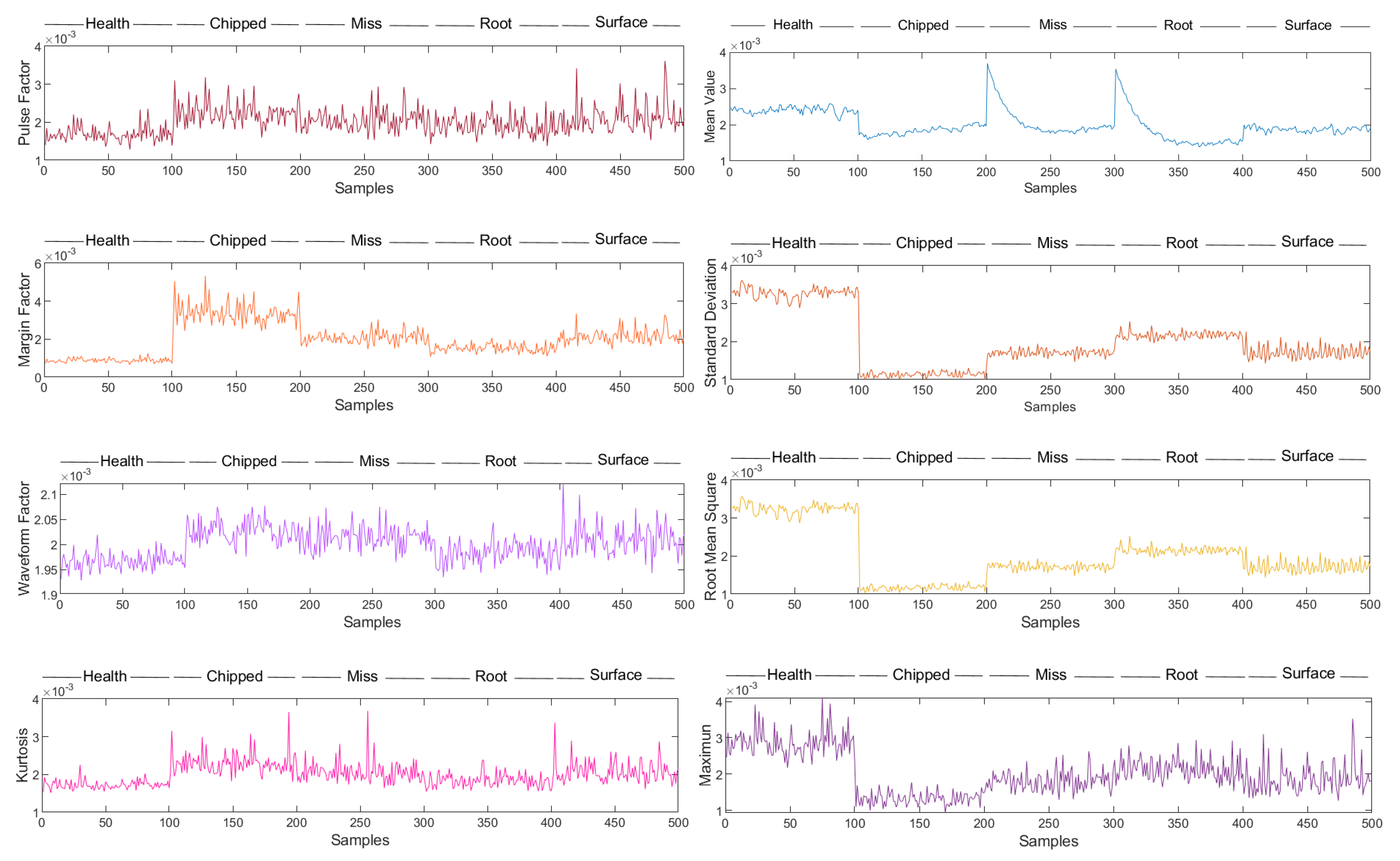
2.1. Time-Domain Features

Since the time-domain signal of gears tends to change when they are faulty, the time-domain characteristic parameters of the gear vibration signal can be analyzed to make an effective diagnosis of the type of fault.

Dimensional time-domain characteristic parameters and dimensionless time-domain characteristic parameters are two commonly used time-domain characteristic parameters. The 13 dimensional and dimensionless time-domain characteristic parameters extracted in this study and their calculation formulas are shown in

Table 1. The 13 time-domain characteristic parameters and their calculation formulas.

Dimensional	Formula	Dimensionless	Formula
Mean Value	$\overline{\mathrm{x}}=\frac{1}{\mathrm{N}}{\displaystyle \sum _{\mathrm{n}=1}^{\mathrm{N}}}\mathrm{x}\left(\mathrm{n}\right)$	Pulse Factor	$\mathrm{I}=\frac{\mathrm{m}\mathrm{a}\mathrm{x}\left|\mathrm{x}\left(\mathrm{n}\right)\right|}{\overline{\mathrm{x}}}$
Standard Deviation	${\mathsf{\sigma }}_{\mathrm{x}}=\sqrt{\frac{1}{\mathrm{N}-1}{\displaystyle \sum _{\mathrm{n}=1}^{\mathrm{N}}}{\left[\mathrm{x}\left(\mathrm{n}\right)-\overline{\mathrm{x}}\right]}^2}$	Margin Factor	$\mathrm{L}=\frac{\mathrm{m}\mathrm{a}\mathrm{x}\left|\mathrm{x}\left(\mathrm{n}\right)\right|}{{\left(\frac{1}{\mathrm{N}}\sum _{\mathrm{n}=1}^{\mathrm{N}}\sqrt{\left|\mathrm{x}\left(\mathrm{n}\right)\right|}\right)}^2}$
Root-Mean-Square Value	${\mathrm{x}}_{\mathrm{r}\mathrm{m}\mathrm{s}}=\sqrt{\frac{1}{\mathrm{N}}{\displaystyle \sum _{\mathrm{n}=1}^{\mathrm{N}}}{\mathrm{x}}^2\left(\mathrm{n}\right)}$	Waveform Factor	$\mathrm{W}=\frac{{\mathrm{x}}_{\mathrm{r}\mathrm{m}\mathrm{s}}}{\overline{\mathrm{x}}}$
Maximum Value	${\mathrm{x}}_{\mathrm{m}\mathrm{a}\mathrm{x}}=\mathrm{m}\mathrm{a}\mathrm{x}\left({\mathrm{x}}_{\mathrm{n}}\right)$	Kurtosis	$\mathrm{K}=\frac{{\sum _{\mathrm{n}=1}^{\mathrm{N}}\left[\mathrm{x}\left(\mathrm{n}\right)-\overline{\mathrm{x}}\right]}^4}{(\mathrm{N}-1){\mathsf{\sigma }}_{\mathrm{x}}^4}$
Minimum Value	${\mathrm{x}}_{\mathrm{m}\mathrm{i}\mathrm{n}}=\mathrm{m}\mathrm{i}\mathrm{n}\left({\mathrm{x}}_{\mathrm{n}}\right)$	Skewness	$\mathrm{S}=\frac{{\sum _{\mathrm{n}=1}^{\mathrm{N}}\left[\mathrm{x}\left(\mathrm{n}\right)-\overline{\mathrm{x}}\right]}^3}{(\mathrm{N}-1){\mathsf{\sigma }}_{\mathrm{x}}^3}$
Peak-peak Value	${\mathrm{x}}_{\mathrm{p}\mathrm{p}}={\mathrm{x}}_{\mathrm{m}\mathrm{a}\mathrm{x}}-{\mathrm{x}}_{\mathrm{m}\mathrm{i}\mathrm{n}}$	Amplitude Factor	$\mathrm{A}=\frac{{\mathrm{x}}_{\mathrm{m}\mathrm{a}\mathrm{x}}}{{\mathrm{x}}_{\mathrm{r}\mathrm{m}\mathrm{s}}}$
		Energy	$\mathrm{E}={\sum }_{\mathrm{n}=1}^{\mathrm{N}}{\mathrm{x}\left(\mathrm{n}\right)}^2$

Note: where x(n) represents the time-domain sequence of the signal, n = 1, 2, …, N; N is the sample number.

[27].

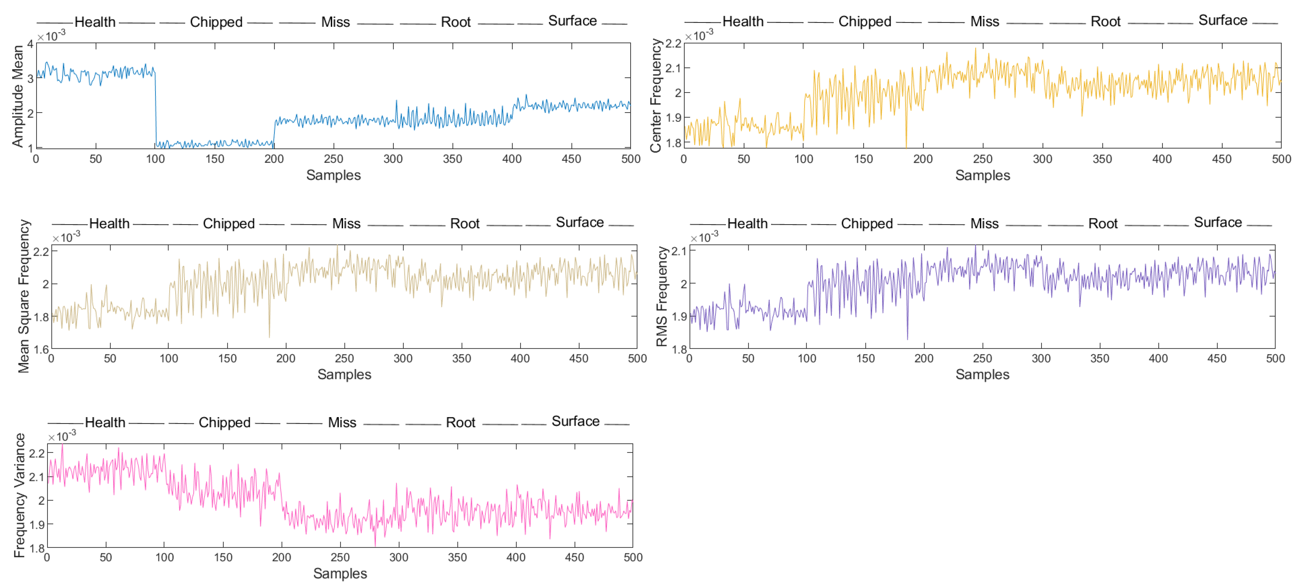
2.2. Frequency-Domain Features

Extracting and analyzing the frequency-domain characteristic parameters of the gear fault vibration signal is also one of the efficient methods for gear fault diagnosis.

Therefore, in this study, the original time-domain vibration signal is transformed into the frequency domain using Fourier transform to observe the characteristics of the vibration signal from the perspective of frequency. The conversion from time-domain to frequency-domain can be defined as:

$$\mathrm{s}\left(\mathrm{k}\right)=\sum _{\mathrm{k}=0}^{\mathrm{N}-1}\mathrm{x}\left(\mathrm{k}∆\mathrm{t}\mathrm{z}\right){\mathrm{e}}^{\frac{-2\mathsf{\pi }\mathrm{j}\mathrm{n}\mathrm{k}}{\mathrm{N}}},\left(\mathrm{n}=\mathrm{1,2},\dots ,\mathrm{N}-1\right)$$

(1)

where $\mathrm{x}\left(\mathrm{k}∆\mathrm{t}\mathrm{z}\right)$ represents the sample value; N denotes the number of sample points; ∆t indicates the sampling interval; k refers to the discrete value of the time-domain signal.

After conversion into frequency signals, the corresponding frequency-domain characteristic parameters can be calculated according to the corresponding frequency-domain statistical index formula. The five frequency-domain characteristic parameters extracted in this study and their calculation formulas are shown in

Table 2. The five frequency-domain characteristic parameters and their calculation formulas.

Frequency Domain Characteristic Parameters	Formula
Amplitude Mean	$\mathrm{A}\mathrm{M}=\frac{1}{\mathrm{K}}{\displaystyle \sum _{\mathrm{k}=1}^{\mathrm{K}}}\mathrm{s}\left(\mathrm{k}\right)$
Center Frequency	$\mathrm{C}\mathrm{F}=\frac{\sum _{\mathrm{k}=1}^{\mathrm{K}}{\mathrm{f}}_{\mathrm{k}·}\mathrm{s}\left(\mathrm{k}\right)}{\sum _{\mathrm{k}=1}^{\mathrm{K}}\mathrm{s}\left(\mathrm{k}\right)}$
Mean Square Frequency	$\mathrm{M}\mathrm{S}\mathrm{F}=\frac{\sum _{\mathrm{k}=1}^{\mathrm{K}}{{\mathrm{f}}_{\mathrm{k}}}^2\mathrm{s}\left(\mathrm{k}\right)}{\sum _{\mathrm{k}=1}^{\mathrm{K}}\mathrm{s}\left(\mathrm{k}\right)}$
Root-Mean-Square Frequency	$\mathrm{R}\mathrm{M}\mathrm{S}\mathrm{F}=\sqrt{\frac{\sum _{\mathrm{k}=1}^{\mathrm{K}}{{\mathrm{f}}_{\mathrm{k}}}^2\mathrm{s}\left(\mathrm{k}\right)}{\sum _{\mathrm{k}=1}^{\mathrm{K}}\mathrm{s}\left(\mathrm{k}\right)}}$
Frequency Variance	$\mathrm{F}\mathrm{V}\mathrm{A}\mathrm{R}=\frac{\sum _{\mathrm{k}=1}^{\mathrm{K}}{{(\mathrm{f}}_{\mathrm{k}}-\mathrm{C}\mathrm{F})}^2·\mathrm{s}\left(\mathrm{k}\right)}{\sum _{\mathrm{k}=1}^{\mathrm{K}}\mathrm{s}\left(\mathrm{k}\right)}$

Note: Where s(k) stands for the spectrum of signal x(n), k = 1, 2, …, K; K is the number of spectral lines; ${\mathrm{f}}_{\mathrm{k}}$ denotes the frequency value of the k-th spectral line.

[28].

2.3. Fusion Features

Extract the above 13 time-domain features and 5 frequency-domain features to form the time-domain feature vector matrix T and the frequency-domain feature vector matrix F, respectively. Assuming that the total number of samples is n, then:

$$\mathrm{T}=\left[\begin{array}{ccc}{\mathrm{t}}_{\mathrm{1,1}}& \cdots & {\mathrm{t}}_{\mathrm{13,1}}\\ ⋮& \ddots & ⋮\\ {\mathrm{t}}_{1,\mathrm{n}}& \dots & {\mathrm{t}}_{13,\mathrm{n}}\end{array}\right]$$

(2)

$$\mathrm{F}=\left[\begin{array}{ccc}{\mathrm{f}}_{\mathrm{1,1}}& \cdots & {\mathrm{f}}_{\mathrm{5,1}}\\ ⋮& \ddots & ⋮\\ {\mathrm{f}}_{1,\mathrm{n}}& \dots & {\mathrm{f}}_{5,\mathrm{n}}\end{array}\right]$$

(3)

The above time-domain feature vector matrix T and frequency-domain feature vector matrix F are fused to form the fused feature vector TF, then:

$$\mathrm{T}\mathrm{F}=\left[\begin{array}{ccc}{\mathrm{x}}_{\mathrm{1,1}}& \cdots & {\mathrm{x}}_{\mathrm{18,1}}\\ ⋮& \ddots & ⋮\\ {\mathrm{x}}_{1,\mathrm{n}}& \dots & {\mathrm{x}}_{18,\mathrm{n}}\end{array}\right]$$

(4)

3. GSWOA-KELM Fault Diagnosis Model

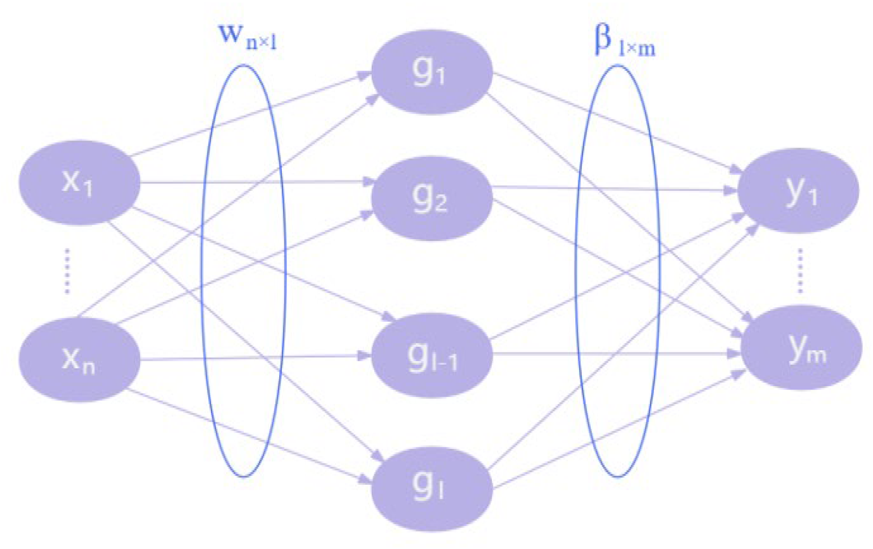
3.1. Kernel Extreme Learning Machine

The KELM is an improved algorithm developed on the basis of an extreme learning machine (ELM). It introduces a kernel function on the basis of an ELM, has better generalization performance, and has a faster learning ability [29].

The ELM is a feed-forward neural network including input, hidden, and output layers [20], and its typical neural network structure is given in Figure 1.

The mathematical expression of an ELM is as follows:

$$\mathrm{H}\mathsf{\beta }=\mathrm{T}$$

(5)

$$\mathrm{H}\left({\mathrm{w}}_1,\dots ,{\mathrm{w}}_{\mathrm{l}},{\mathrm{b}}_1,\dots ,{\mathrm{b}}_{\mathrm{l}},{\mathrm{x}}_1,\dots ,{\mathrm{x}}_{\mathrm{n}}\right)=\left(\begin{array}{ccc}\mathrm{g}({\mathrm{w}}_1·{\mathrm{x}}_1+{\mathrm{b}}_1)& \cdots & \mathrm{g}({\mathrm{w}}_{\mathrm{l}}·{\mathrm{x}}_1+{\mathrm{b}}_{\mathrm{l}})\\ ⋮& \ddots & ⋮\\ \mathrm{g}({\mathrm{w}}_1·{\mathrm{x}}_{\mathrm{n}}+{\mathrm{b}}_{\mathrm{l}})& \cdots & \mathrm{g}({\mathrm{w}}_{\mathrm{l}}·{\mathrm{x}}_{\mathrm{n}}+{\mathrm{b}}_{\mathrm{l}})\end{array}\right)$$

(6)

where $\mathrm{H}$ represents the output matrix of the hidden layer, $\mathsf{\beta }$ is the output weight, $\mathrm{T}$ denotes the target output matrix, $w_l$ is the weight of the $\mathrm{l}$-th neuron in the hidden layer, and $b_l$ denotes the bias of the $\mathrm{l}$-th neuron in the hidden layer.

The learning process of an ELM is the process of solving the output weight β, which is solved using the least squares method:

$${\mathsf{\beta }}_{\mathrm{E}\mathrm{L}\mathrm{M}}={\mathrm{H}}^{\mathrm{T}}{\left({\mathrm{H}\mathrm{H}}^{\mathrm{T}}\right)}^{-1}\mathrm{T}={\mathrm{H}}^{+}\mathrm{T}$$

(7)

where ${\mathrm{H}}^{+}$ represents the generalized inverse matrix of $\mathrm{H}$.

In KELM, the regularization coefficient C and kernel function parameters γ are introduced to improve the performance of the KELM, and the kernel function matrix is expressed as:

$$\mathsf{\Omega }=\mathrm{H}{\mathrm{H}}^{\mathrm{T}}$$

(8)

$${\mathsf{\Omega }}_{\mathrm{i}\mathrm{j}}=\mathrm{h}\left({\mathrm{x}}_{\mathrm{i}}\right)\mathrm{h}\left({\mathrm{x}}_{\mathrm{j}}\right)=\mathrm{K}({\mathrm{x}}_{\mathrm{i}},{\mathrm{x}}_{\mathrm{j}})$$

(9)

Then, the least square solution of the β value of the KELM is:

$${\mathsf{\beta }}_{\mathrm{K}\mathrm{E}\mathrm{L}\mathrm{M}}={\mathrm{H}}^{\mathrm{T}}{\left(\frac{\mathrm{I}}{\mathrm{C}}+\mathrm{H}{\mathrm{H}}^{\mathrm{T}}\right)}^{-1}\mathrm{T}$$

(10)

Based on the above equations, the output function of the KELM can be expressed as:

$$\mathrm{f}\left(\mathrm{x}\right)=\left[\begin{array}{c}\begin{array}{c}\mathrm{K}\left(\mathrm{x},{\mathrm{x}}_1\right)\\ ⋮\end{array}\\ \mathrm{K}\left(\mathrm{x},{\mathrm{x}}_{\mathrm{n}}\right)\end{array}\right]{(\mathsf{\Omega }+\frac{\mathrm{I}}{\mathrm{C}})}^{-1}\mathrm{T}$$

(11)

In addition, the radial basis function (RBF) is chosen as the kernel function in this research, whose expression is as follows:

$$\mathrm{K}\left({\mathrm{x}}_{\mathrm{i}},{\mathrm{x}}_{\mathrm{j}}\right)=\mathrm{e}\mathrm{x}\mathrm{p}\left(-\frac{{\left|\left|{\mathrm{x}}_{\mathrm{i}}-{\mathrm{x}}_{\mathrm{j}}\right|\right|}^2}{{2\mathsf{\gamma }}^2}\right)$$

(12)

where $\mathsf{\gamma }$ is the kernel parameter.

3.2. Whale Optimization Algorithm

The WOA is a swarm intelligence optimization algorithm that imitates the hunting process of whales in nature, which can be divided into three stages: the encircling prey stage, the bubble-net attacking stage, and the random hunting prey stage [30,31]. In each stage, the position of the whale is updated. The process of using the whale optimization algorithm to solve the problem is to represent the position of each whale as a feasible solution and obtain the optimal solution by constantly updating the position of the whale.

During the encircling prey phase, the whale’s position update formula can be expressed as:

$$\left\{\begin{array}{c}\mathsf{X}\left(\mathrm{t}+1\right)={\mathrm{X}}^{\mathrm{*}} \left(\mathrm{t}\right)-\mathsf{A}·\mathsf{D}\\ \mathsf{D}=\left|\mathrm{C}·{\mathrm{X}}^{\mathrm{*}}\left(\mathrm{t}\right)-\mathrm{X}\left(\mathrm{t}\right)\right|\end{array}\right.$$

(13)

where $\mathrm{t}$ represents the number of iterations; $\mathrm{X}\left(\mathrm{t}\right)$ indicates the current position of the whale; ${\mathrm{X}}^{\mathrm{*}}\left(\mathrm{t}\right)$ represents the optimal whale location; $\mathrm{D}$ is the distance between the whale and the prey; and $\mathrm{A}$ and $\mathrm{C}$ represent the coefficient, whose expression is:

$$\left\{\begin{array}{c}\mathsf{A}=2\mathsf{a}·{\mathrm{r}}_1-\mathsf{a}\\ \mathsf{C}=2{\mathrm{r}}_2\\ \mathsf{a}=2-2\mathsf{t}/{\mathrm{t}}_{\mathrm{m}\mathrm{a}\mathrm{x}}\end{array}\right.$$

(14)

During the bubble-net attacking phase, the position update of the whale can be described using two mechanisms, namely, the contraction surround mechanism and the spiral update mechanism. The mathematical expression of the spiral update mechanism is

$$\left\{\begin{array}{c}\mathrm{X}(\mathrm{t}+1)={\mathrm{X}}^{\mathrm{*}} \left(\mathrm{t}\right)+\mathrm{D}·{\mathrm{e}}^{\mathrm{b}\mathrm{l}} \mathrm{c}\mathrm{o}\mathrm{s}\left(2\mathsf{\pi }\mathrm{l}\right)\\ \mathrm{D}=|\mathrm{C}·{\mathrm{X}}^{\mathrm{*}} (\mathrm{t})-\mathrm{X}(\mathrm{t}\left)\right|\end{array}\right.$$

(15)

where $\mathrm{l}$ represents the random number in the range between 0 and 1; $\mathrm{b}$ is a constant that reflects the shape of the helix.

It is worth noting that during the bubble-net attacking stage, the whale not only approaches the prey in a spiral shape but also shrinks the encircling circle, which is then mathematically modeled as:

$$\mathrm{X}\left(\mathrm{t}+1\right)=\left\{\begin{array}{c}{\mathrm{X}}^{\mathrm{*}}\left(\mathrm{t}\right)-\mathsf{A}·\left|\mathrm{C}·{\mathrm{X}}^{\mathrm{*}}\left(\mathrm{t}\right)-\mathrm{X}\left(\mathrm{t}\right)\right|,p<0.5\\ {\mathrm{X}}^{\mathrm{*}}\left(\mathrm{t}\right)+\mathsf{D}·{\mathrm{e}}^{\mathrm{b}\mathrm{l}}\cos \left(2\mathsf{\pi }\mathrm{l}\right),p\ge 0.5\end{array}\right.$$

(16)

where $p$ represents random numbers in the range between 0 and 1.

During the prey search phase, whales use a random search mechanism to search for prey globally. At this time, the updating method of whale position is determined by the range of A: if |A| < 1, the position is updated by spiral encircling; if |A|≥1, the location is updated by random search. The mathematical model of the random search mechanism updating location is

$$\mathrm{X}\left(\mathrm{t}+1\right)={\mathrm{X}}_{\mathrm{r}\mathrm{a}\mathrm{n}\mathrm{d}}\left(\mathrm{t}\right)-\mathrm{A}·|\mathrm{C}·{\mathrm{X}}_{\mathrm{r}\mathrm{a}\mathrm{n}\mathrm{d}}\left(\mathrm{t}\right)-\mathrm{X}\left(\mathrm{t}\right)|$$

(17)

where ${\mathrm{X}}_{\mathrm{r}\mathrm{a}\mathrm{n}\mathrm{d}}\left(\mathrm{t}\right)$ denotes the position of a random whale.

3.3. Global Search Whale Optimization Algorithm

In order to improve the convergence speed and global search ability of traditional whale optimization algorithms, an improved global search whale optimization algorithm (GSWOA) is proposed based on three strategies, namely, adaptive weight strategy, variable spiral position update strategy, and optimal neighborhood perturbation strategy [32].

First, the adaptive weight strategy is to introduce an adaptive inertia weight based on the number of iterations t into the position update of the whale, and its expression is as follows:

$$\mathrm{w}\left(\mathrm{t}\right)=0.2\cos \left(\frac{\mathsf{\pi }}{2}·\left(1-\frac{\mathrm{t}}{{\mathrm{t}}_{\mathrm{m}\mathrm{a}\mathrm{x}}}\right)\right)$$

(18)

where w(t) is the adaptive inertia weight, and the variation range is [0, 1]; t is the current iteration number; and ${\mathrm{t}}_{\mathrm{m}\mathrm{a}\mathrm{x}}$ indicates the maximum iteration number.

According to Equation (18), in the early stage of the algorithm, the weight value is small but changes quickly; in the later stage of the algorithm, with the increase in the number of iterations, the weight is large, but the change speed slows down, thus improving the convergence of the algorithm.

The position update formula of the improved whale optimization algorithm is

$$\mathrm{X}\left(\mathrm{t}+1\right)=\left\{\begin{array}{c}{\mathrm{w}\left(\mathrm{t}\right)·\mathrm{X}}^{\mathrm{*}}\left(\mathrm{t}\right)-\mathsf{A}·\left|\mathrm{C}·{\mathrm{X}}^{\mathrm{*}}\left(\mathrm{t}\right)-\mathrm{X}\left(\mathrm{t}\right)\right|,p<0.5\\ {\mathrm{w}\left(\mathrm{t}\right)·\mathrm{X}}^{\mathrm{*}}\left(\mathrm{t}\right)+\mathsf{D}·{\mathrm{e}}^{\mathrm{b}\mathrm{l}}\cos \left(2\mathsf{\pi }\mathrm{l}\right),p\ge 0.5\end{array}\right.$$

(19)

$$\mathrm{X}\left(\mathrm{t}+1\right)=\mathrm{w}\left(\mathrm{t}\right){\mathrm{X}}_{\mathrm{r}\mathrm{a}\mathrm{n}\mathrm{d}}\left(\mathrm{t}\right)-\mathrm{A}·|\mathrm{C}·{\mathrm{X}}_{\mathrm{r}\mathrm{a}\mathrm{n}\mathrm{d}}(\mathrm{t})-\mathrm{X}\left(\mathrm{t}\right)|$$

(20)

Second, the variable spiral position update strategy refers to changing the constant b, which reflects the spiral shape in the bubble-net attacking stage, to a dynamically adjusted variable based on the number of iterations. The mathematical formula is as follows:

$$\mathrm{b}={\mathrm{e}}^{5·\cos \left(\mathsf{\pi }·\left(1-\frac{\mathrm{t}}{{\mathrm{t}}_{\mathrm{m}\mathrm{a}\mathrm{x}}}\right)\right)}$$

(21)

From Equation (21), it can be seen that in the early phase of the algorithm, the spiral shape range is larger, and the whale can search for optimization in a larger range and has a stronger global search ability; with the increase of the number of iterations, the spiral shape range becomes smaller, and the whale can search in a smaller range to improve the optimization accuracy.

Now, the position update formula of the improved whale optimization algorithm is

$$\mathrm{X}\left(\mathrm{t}+1\right)={\mathrm{w}\left(\mathrm{t}\right)·\mathrm{X}}^{\mathrm{*}}\left(\mathrm{t}\right)+\mathrm{b}\mathrm{D}·{\mathrm{e}}^{\mathrm{b}\mathrm{l}}\mathrm{c}\mathrm{o}\mathrm{s}\left(2\mathsf{\pi }\mathrm{l}\right)$$

(22)

Finally, the optimal neighborhood perturbation strategy is to expand the search scope of the optimal location to the vicinity of the current optimal location when the whale position is updated and search the nearby space simultaneously instead of being limited to the current optimal location. In this way, the search efficiency of the whale and the convergence speed of the algorithm can be enhanced. The mathematical expression for generating a disturbance in the neighborhood of the current optimal location and generating a new location is

$$\widehat{\mathrm{X}}(\mathrm{t})=\left\{\begin{array}{c}{\mathrm{X}}^{\mathrm{*}}\left(\mathrm{t}\right)+0.5·\mathrm{rand}1·{\mathrm{X}}^{\mathrm{*}}\left(\mathrm{t}\right),\mathrm{rand}2<0.5\\ {\mathrm{X}}^{\mathrm{*}}\left(\mathrm{t}\right),\mathrm{rand}2\ge 0.5\end{array}\right.$$

(23)

where $\mathrm{r}\mathrm{a}\mathrm{n}\mathrm{d}1$ and $\mathrm{r}\mathrm{a}\mathrm{n}\mathrm{d}2$ indicate uniform random numbers in the range [0, 1]; $\widehat{\mathrm{X}}\left(\mathrm{t}\right)$ is the generated new location.

If the generated new position is better than the original position, the new position is kept. If the generated new position is inferior to the original position, the original position is retained. The formula is expressed as:

$${\mathrm{X}}^{\mathrm{*}}\left(\mathrm{t}\right)=\left\{\begin{array}{c}\widehat{\mathrm{X}}\left(\mathrm{t}\right), \mathrm{f}\left(\widehat{\mathrm{X}}\left(\mathrm{t}\right)\right)<\mathrm{f}\left({\mathrm{X}}^{\mathrm{*}}\left(\mathrm{t}\right)\right)\\ {\mathrm{X}}^{\mathrm{*}}\left(\mathrm{t}\right),\mathrm{f}\left({\mathrm{X}}^{\mathrm{*}}\left(\mathrm{t}\right)\right)\le \mathrm{f}\left(\widehat{\mathrm{X}}\left(\mathrm{t}\right)\right)\end{array}\right.$$

(24)

where $\mathrm{f}\left(\mathrm{x}\right)$ represents the fitness value when the position is $\mathrm{x}$.

The overall flow of the GSWOA is shown in Figure 2.

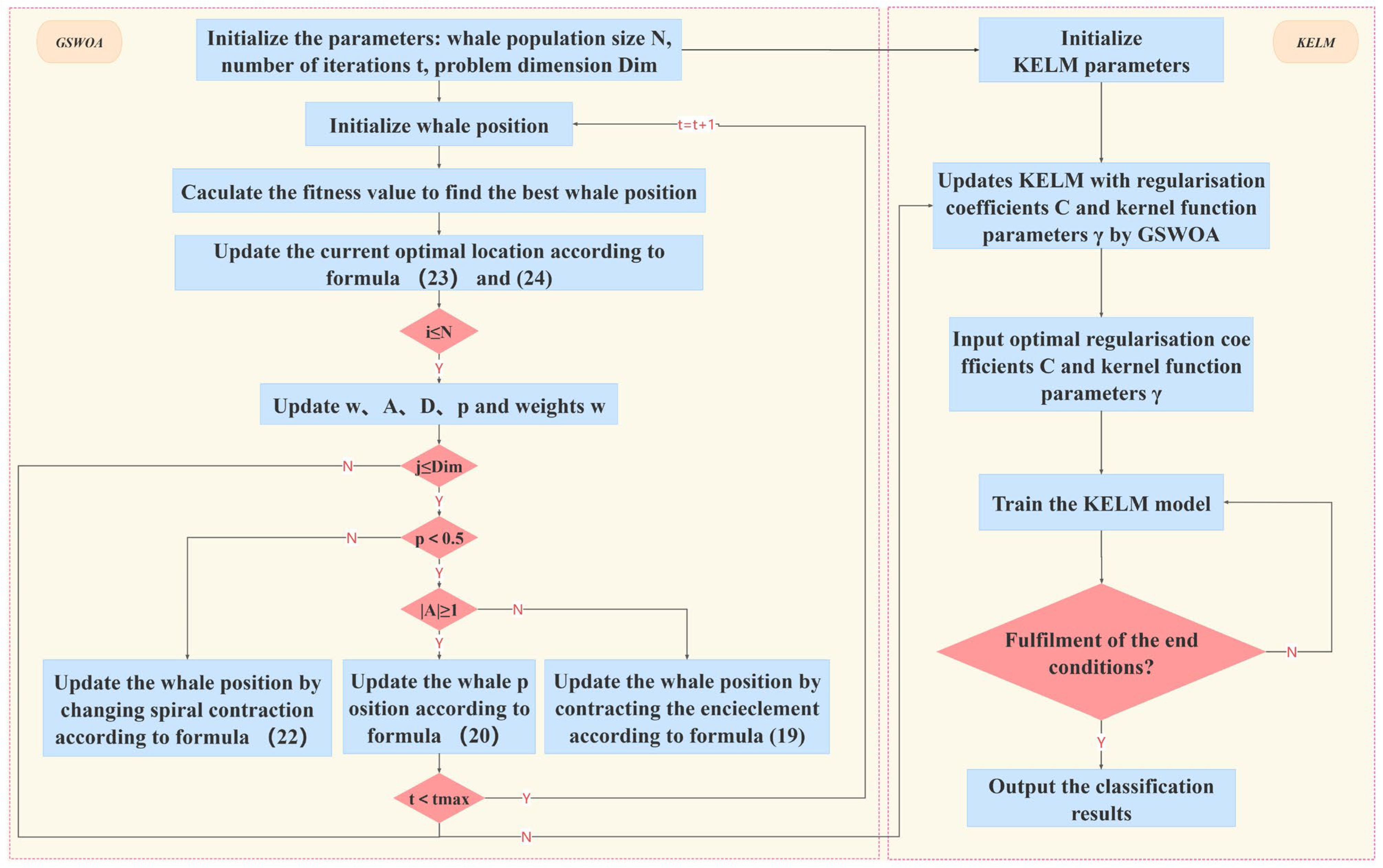
3.4. Kernel Extreme Learning Machine Optimized Using the Global Search Whale Optimization Algorithm

In this study, GSWOA is used to intelligently optimize the regularization coefficient C and kernel function parameter γ of KELM, and a GSWOA-KELM gear fault diagnosis model is constructed to avoid the problem of low fault diagnosis efficiency of KELM caused by artificial parameter selection. The process of using GSWOA to optimize KELM parameters is shown in Figure 3. The specific steps are as follows:

Step 1: Initialize the parameters of the GSWOA, set the whale population size to 10, the maximum number of iterations to 60, the problem dimension to 2, and the whale exploration boundary to [1,20];

Step 2: Initialize the whale position and map it to the initialization parameters of KELM: regularization coefficient C and kernel function parameter γ;

Step 3: Calculate the fitness value of each whale in the whale population and find the optimal whale location in the population;

Step 4: Update the current optimal location using Formulas (23) and (24);

Step 5: Randomly generate the update parameter p. If p < 0.5 and |A| < 1, update the whale position using Formula (16); if p < 0.5 and |A| ≥ 1, use Formula (20) to update the position of the whale. If p ≥ 0.5, the whale position is updated using Formula (22), where A is the step coefficient of the convergence factor optimization;

Step 6: Determine whether the maximum number of iterations has been reached. If it is, output the whale position at this moment as the optimal parameters of KELM, input these optimal parameters into the KELM model, and train the model for fault diagnosis; if not, repeat the above steps until the maximum number of iterations is reached.

4. Experimental Verification and Result Analysis

4.1. Data Acquisition and Preprocessing

The open gearbox fault data set collected from the drivetrain dynamic simulator (DDS) of Southeast University is used to verify the proposed method, whose data acquisition test platform is shown in Figure 4. This test platform includes a brake, brake controller, planetary gearbox, reduction gearbox, motor, motor controller, and other components. Gear bearings are mounted on the second-stage drive shaft of the reduction gearbox or the second-stage planetary shaft of the planetary gearbox, and seven vibration sensors of type 608A11 are mounted in the direction of the x, y, and z-axes of the planetary gearbox and reduction gearbox as well as in the direction of the motor’s z-axis with a sampling frequency of 5120 Hz. Its collected data include two working conditions, with the speed and load of 20 Hz/0 V and 30 Hz/2 V, respectively. There are five types of gear faults: health, chipped, root, miss, and surface. A detailed description of them is shown in

Table 3. Dataset fault type description and classification label.

Fault Type	Fault Description	Classification Label	Sample Number		Total Sample Number
			Train Set	Test Set
Health	Healthy gear.	1	70	30	100
Chipped	The gear is cracked or even broken.	2	70	30	100
Miss	Gear defect.	3	70	30	100
Root	There is a crack at the root of the gear.	4	70	30	100
Surface	Gear surface wear.	5	70	30	100

. The gears of different fault states are processed in advance, the variable speed can be realized via the motor controller, and the change of load is realized via the load controller.

In this study, the data under the 20 Hz/0 V condition are selected for research; each type of fault intercepts 100 sample groups, and each sample group contains 2048 sample points. The data set is randomly divided according to the ratio of the training set to the test set = 7:3, and the labels for the five types of gearbox faults are established, as shown in Table 3.

4.2. Time-Frequency Features Extraction

Thirteen time-domain features described in Table 1 and five frequency-domain features described in Table 2 are extracted and normalized, respectively. The data distributions of different time-domain features and frequency-domain features in different gear fault states are shown in Figure 5 and Figure 6, respectively.

4.3. Fault Diagnosis and Result Analysis

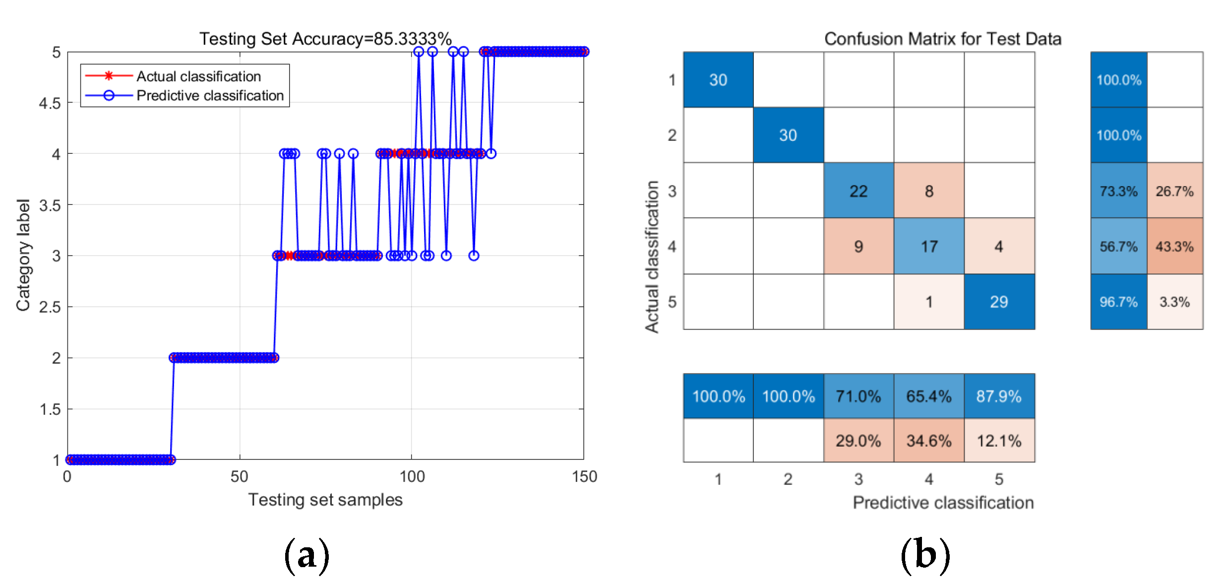
4.3.1. Fault Diagnosis and Result Analysis without Feature Fusion

The time-domain feature matrix T, frequency-domain feature matrix F, and fusion-feature matrix TF obtained after the above feature extraction are input into the GSWOA-KELM fault diagnosis model, respectively. In this model, the number of the whale population is set to 10, the maximum number of iterations is 60, the dimension is 2, the upper bound is 1, and the lower bound is 20. The dataset partitioning and labeling settings are set, as shown in Table 3. The fault diagnosis results under three different inputs are shown in Figure 7, Figure 8 and Figure 9, respectively, where Figure 7a, Figure 8a and Figure 9a shows the comparison results of predicted classification and actual classification, and Figure 7b, Figure 8b and Figure 9b indicates the confusion matrix of classification results. In Figure 7b, Figure 8b and Figure 9b, the blue line indicates the number and proportion of samples correctly classified and the red line indicates the number and proportion of samples misclassified.

The accuracy rate of fault diagnosis under three different inputs is shown in

Table 4. The accuracy rate for different inputs.

Input	Accuracy Rate
T	86.67%
F	85.33%
TF	100%

.

As can be seen from Table 4, the classification accuracy of GSWOA-KELM is lower when the inputs are single-domain features in time-domain or frequency-domain, and the classification accuracy of the training set is 86.67% and 85.33%, respectively, whereas when the inputs are fusion features, GSWOA-KELM has the highest classification accuracy, and the classification accuracy reaches 100%. Compared to when the time domain and frequency domain are used as separate feature vectors, the accuracy is improved by 13.33% and 14.67%. Therefore, extracting multi-domain features of gear faults as inputs to the model can significantly improve the classification accuracy of the fault diagnosis model.

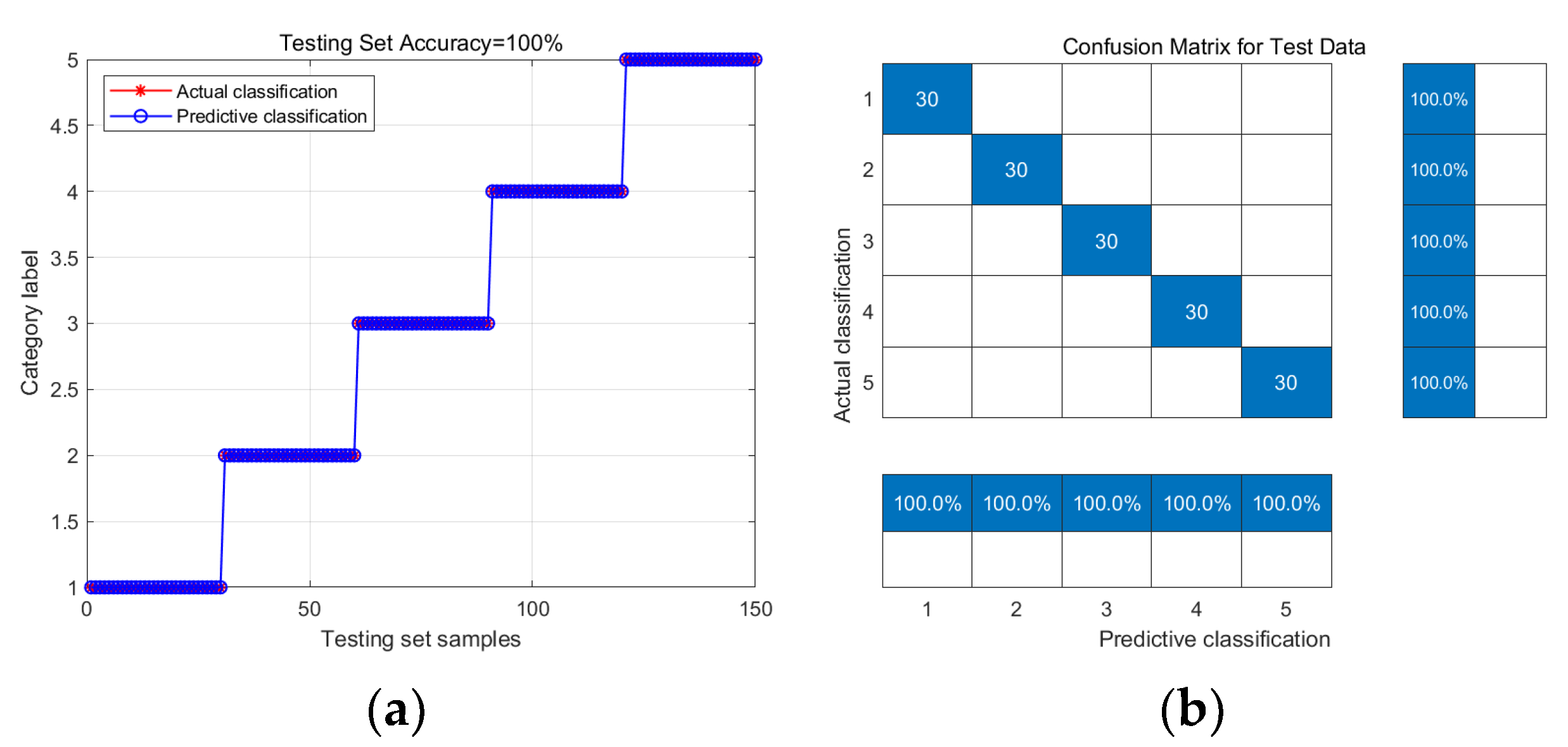
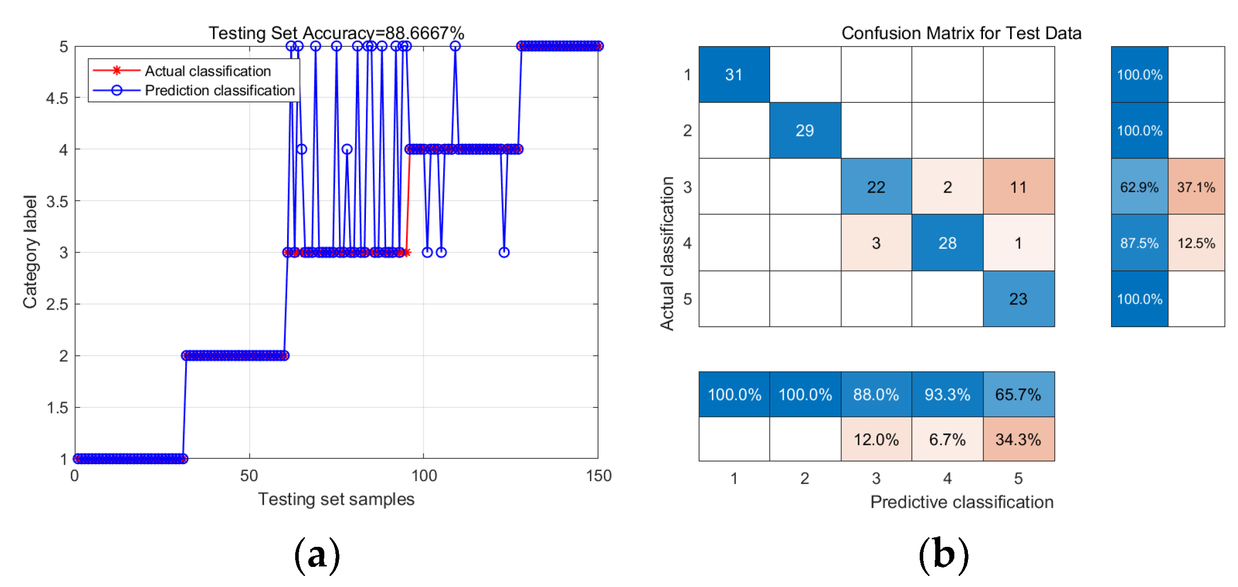
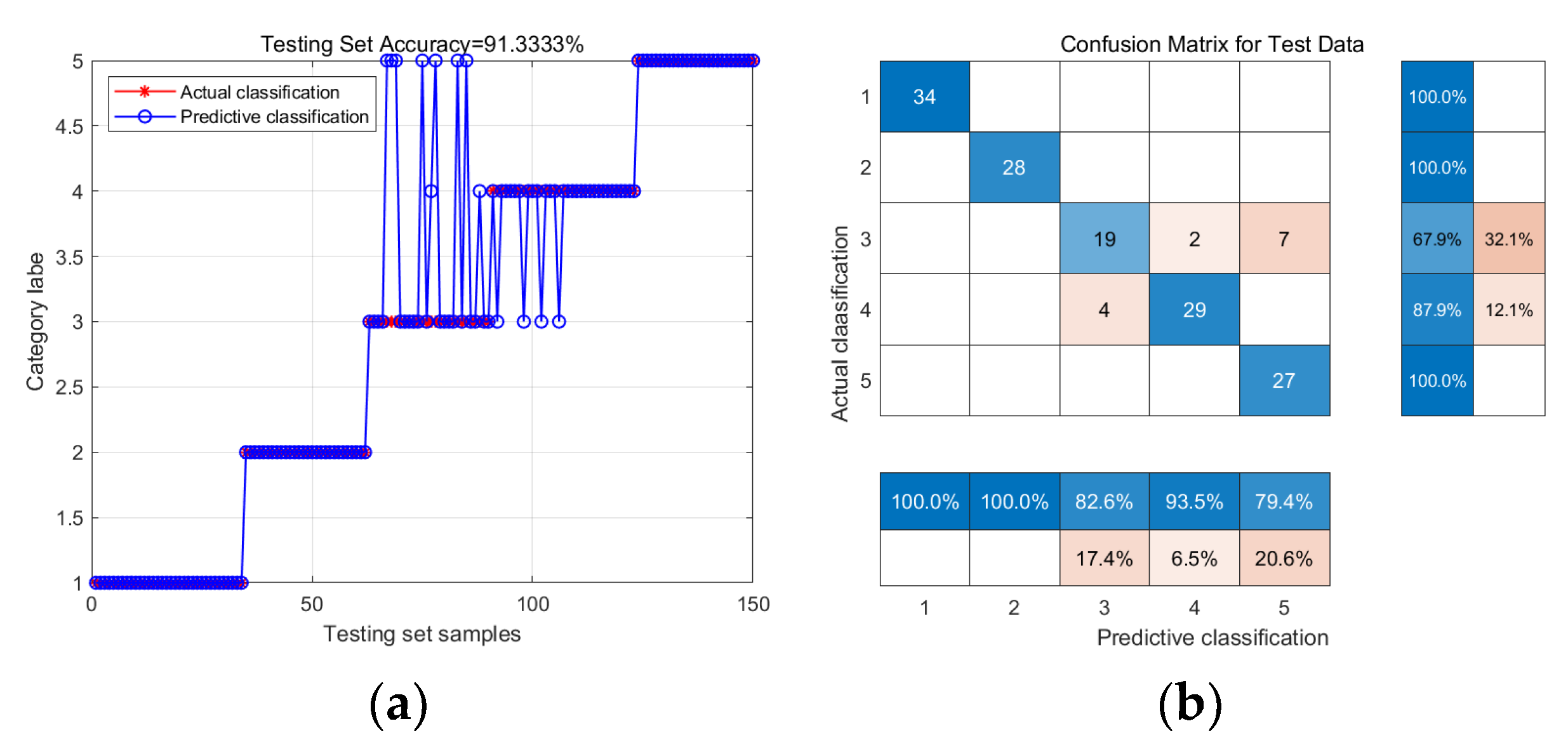
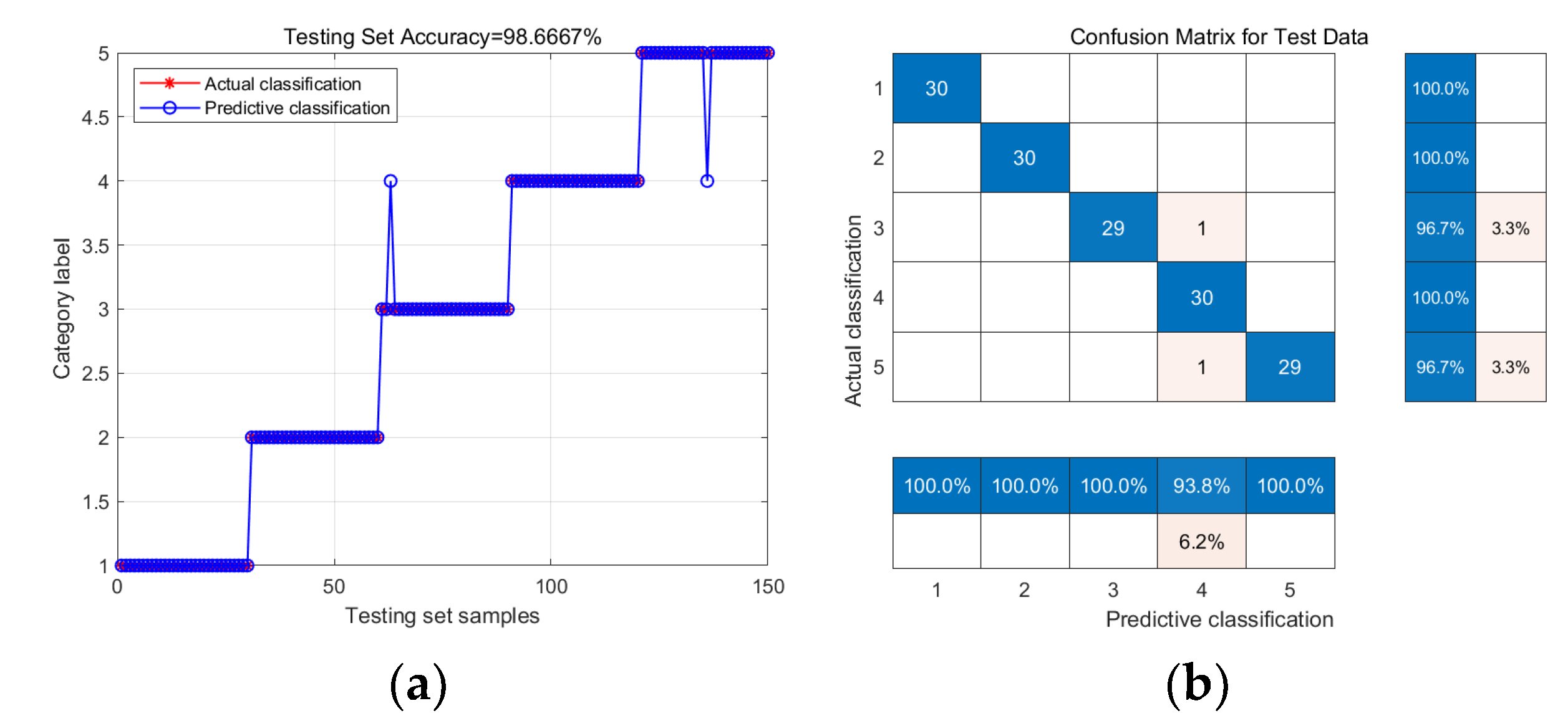
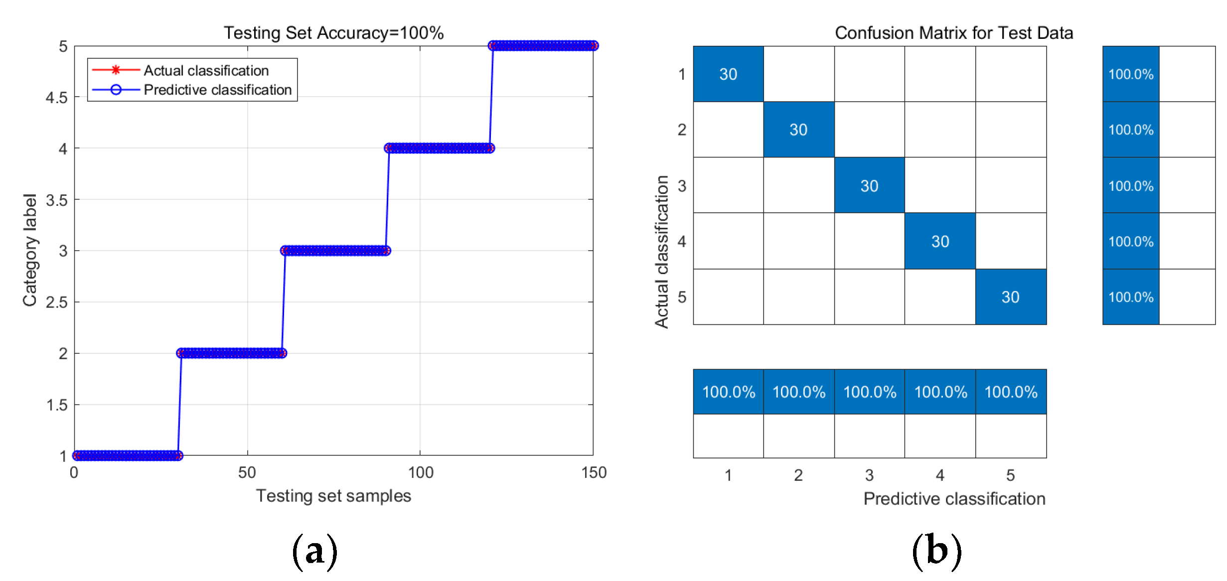
4.3.2. Fault Diagnosis and Result Analysis with Feature Fusion

First, in order to verify the superiority of the GSWOA-KELM model in terms of convergence speed and global search performance, the fusion feature vector TF is input into the SSA-KELM, WOA-KELM, and GSWOA-KELM fault diagnosis models, respectively, and the fitness curves of the three models are compared, as shown in Figure 10. During fault diagnosis, the parameters of the three models are set to be consistent, where the population number is 10, the maximum number of iterations is 60, and the dimension is 2. The dataset partitioning and label setting are set as shown in Table 3.

Figure 10a shows the algorithm converges after 50 iterations, and the final convergence value is 0.098. Figure 10b shows that when WOA is used to optimize KELM, its fitness curve is a straight line, which is analyzed because the model falls into local optimality from the beginning. As shown in Figure 10c, GSWOA-KELM only iterates twice to find the optimal value, and the final convergence value is 0, which is lower than the final convergence value of SSA-KELM, with faster convergence speed and higher optimization accuracy. Meanwhile, compared with WOA-KELM, GSWOA-KELM avoids premature convergence and local optimization and has a stronger global search ability.

Next, in order to verify the fault diagnosis accuracy of the GSWOA-KELM model, KELM, SSA-KELM, and WOA-KELM models are selected for comparison and verification. At first, the fusion feature vector TF is input into the above four fault diagnosis models respectively, in which the population number of SSA, WOA, and GSWOA optimization algorithms is set as 10, the maximum number of iterations is 60, and the dimension is two-dimensional. What is more, the dataset partitioning and label settings are set, as shown in Table 3. The classification accuracy rate of each fault diagnosis model is shown in

Table 5. The classification accuracy rate of each fault diagnosis model.

Fault Diagnosis Model	Fault Type	Accuracy Rate	Overall Accuracy
KELM	Health	100%	88.67%
	Chipped	100%
	Miss	88.0%
	Root	93.3%
	Surface	65.7%
SSA-KELM	Health	100%	91.33%
	Chipped	100%
	Miss	82.6%
	Root	83.5%
	Surface	79.4%
WOA-KELM	Health	100%	98.67%
	Chipped	100%
	Miss	100%
	Root	100%
	Surface	96.8%
GSWOA-KELM	Health	100%	100%
	Chipped	100%
	Miss	100%
	Root	100%
	Surface	100%

. The fault diagnosis results of each model are shown in Figure 11, Figure 12, Figure 13 and Figure 14, where Figure 11a, Figure 12a, Figure 13a and Figure 14a is the comparison results of the predicted classification and the actual classification of each model, and Figure 11b, Figure 12b, Figure 13b and Figure 14b shows the confusion matrix of the classification results of each model.

As shown in Table 5, the fault diagnosis classification accuracies of KELM, SSA-KELM, WOA-KELM, and GSWOA-KELM models are 88.67%, 91.33%, 98.67%, and 100%, respectively. Among them, GSWOA-KELM, established in this study, has the highest accuracy, which reaches 100%. Compared with the other three models, the fault diagnosis classification accuracy of GSWOA-KELM is improved by 11.33%, 8.67%, and 1.33%, respectively.

As can be seen from Figure 11, Figure 12, Figure 13 and Figure 14, the GSWOA-KELM model can accurately identify various fault types and has no misclassification. Compared with GSWOA-KELM, the misclassified fault types of the other three models mainly focus on Miss and Surface. Figure 11 denotes that, in the KELM model, three Root samples are misclassified as Miss samples, one Root sample is misclassified as Surface samples, and two Miss samples are misclassified as Root samples. Figure 12 indicates that in the SSA-KELM model, four Root samples are misclassified as Miss samples, two Miss samples are misclassified as Root samples, and seven Miss samples are misclassified as Surface samples. As can be seen from Figure 13, in the WOA-KELM model, one Miss sample and one Surface sample are misclassified as Root samples separately.

5. Conclusions

Aiming at the problem of low accuracy caused via manual parameter selection in KELM fault diagnosis, an improved time-frequency fusion features-based GSWOA-KELM model is proposed. The results have confirmed that the model proposed in this study has the ideal effect on gear fault diagnosis. The specific conclusions are as follows:

(1)

Compared with KELM, SSA-KELM, and WOA-KELM, the GSWOA-KELM has faster convergence speed, stronger global search capability, and higher recognition accuracy;

(2)

When constructing a GSWOA-KELM model for gear fault diagnosis, the GSWOA-KELM performance can be improved by considering the fusion features rather than the single time-domain or frequency-domain features;

(3)

Compared to KELM, SSA-KELM, and WOA-KELM, the GSWOA-KELM model proposed in this study improved the fault diagnosis accuracy by 11.33%, 8.67%, and 1.33%, respectively.

Since real-world gear systems usually have different signal-to-noise ratios, the proposed method needs to be tested in more practical engineering application scenarios. In the next step, it is necessary to study the applicability of the proposed method under different signal-to-noise ratios and port the proposed algorithm to an embedded terminal to realize on-line diagnosis of gear faults [10].

References

1. Hagemann, T.; Ding, H.; Radtke, E.; Schwarze, H. Operating Behavior of Sliding Planet Gear Bearings for Wind Turbine Gearbox Applications—Part II: Impact of Structure Deformation. Lubricants 2021, 9, 98. [Google Scholar] [CrossRef]
2. Issaadi, I.; Hemsas, K.E.; Soualhi, A. Wind Turbine Gearbox Diagnosis Based on Stator Current. Energies 2023, 16, 5286. [Google Scholar] [CrossRef]
3. Shi, Z.; Liu, S.; Yue, H.; Wu, X. Noise Analysis and Optimization of the Gear Transmission System for Two-Speed Automatic Transmission of Pure Electric Vehicles. Mech. Sci. 2023, 14, 333–345. [Google Scholar] [CrossRef]
4. Vasić, M.P.; Stojanović, B.; Blagojević, M. Fault Analysis of Gearboxes in Open Pit Mine. Appl. Eng. Lett. 2020, 5, 50–61. [Google Scholar] [CrossRef]
5. Bai, Z.; Ning, Z. Dynamic Responses of the Planetary Gear Mechanism Considering Dynamic Wear Effects. Lubricants 2023, 11, 255. [Google Scholar] [CrossRef]
6. De las Morenas, J.; Moya-Fernández, F.; López-Gómez, J.A. The Edge Application of Machine Learning Techniques for Fault Diagnosis in Electrical Machines. Sensors 2023, 23, 2649. [Google Scholar] [CrossRef] [PubMed]
7. Ma, G.; Yue, X.; Zhu, J.; Liu, Z.; Lu, S. Deep Learning Network Based on Improved Sparrow Search Algorithm Optimization for Rolling Bearing Fault Diagnosis. Mathematics 2023, 11, 4634. [Google Scholar] [CrossRef]
8. Liu, H.; Song, X.; Zhang, F. Fault diagnosis of new energy vehicles based on improved machine learning. Soft Comput. 2021, 25, 12091–12106. [Google Scholar] [CrossRef]
9. Zhang, C.; Peng, Z.; Chen, S.; Li, Z.; Wang, J. A Gearbox Fault Diagnosis Method Based on Frequency-Modulated Empirical Mode Decomposition and Support Vector Machine. Proc. Inst. Mech. Eng. Part C J. Mech. Eng. Sci. 2018, 232, 369–380. [Google Scholar] [CrossRef]
10. Wang, H.; Yu, Z.; Guo, L. Real-Time Online Fault Diagnosis of Rolling Bearings Based on KNN Algorithm. J. Phys. Conf. Ser. 2020, 1486, 032019. [Google Scholar] [CrossRef]
11. Yuan, L.; Lian, D.; Kang, X.; Chen, Y.; Zhai, K. Rolling Bearing Fault Diagnosis Based on Convolutional Neural Network and Support Vector Machine. IEEE Access 2020, 8, 137395–137406. [Google Scholar] [CrossRef]
12. Zhang, Y.; Jia, Y.; Wu, W.; Cheng, Z.; Su, X.; Lin, A. A Diagnosis Method for the Compound Fault of Gearboxes Based on Multi-Feature and BP-AdaBoost. Symmetry 2020, 12, 461. [Google Scholar] [CrossRef]
13. Zhang, W.; Lu, H.; Zhang, Y.; Li, Z.; Wang, Y.; Zhou, J.; Mei, J.; Wei, Y. A Fault Diagnosis Scheme for Gearbox Based on Improved Entropy and Optimized Regularized Extreme Learning Machine. Mathematics 2022, 10, 4585. [Google Scholar] [CrossRef]
14. Bai, X.; Ma, Z.; Chen, W.; Wang, S.; Fu, Y. Fault Diagnosis Research of Laser Gyroscope Based on Optimized-Kernel Extreme Learning Machine. Comput. Electr. Eng. 2023, 111, 108956. [Google Scholar] [CrossRef]
15. Liang, R.; Chen, Y.; Zhu, R. A Novel Fault Diagnosis Method Based on the KELM Optimized by Whale Optimization Algorithm. Machines 2022, 10, 93. [Google Scholar] [CrossRef]
16. Li, X.; Fang, Y.; Liu, L. Kernel Extreme Learning Machine for Flatness Pattern Recognition in Cold Rolling Mill Based on Particle Swarm Optimization. J. Braz. Soc. Mech. Sci. Eng. 2020, 42, 270. [Google Scholar] [CrossRef]
17. Song, C.; Yao, L.; Hua, C.; Ni, Q. Comprehensive Water Quality Evaluation Based on Kernel Extreme Learning Machine Optimized with the Sparrow Search Algorithm in Luoyang River Basin, China. Environ. Earth Sci. 2021, 80, 521. [Google Scholar] [CrossRef]
18. Zhou, F.; Gong, J.; Yang, X.; Han, T.; Yu, Z. A New Gear Intelligent Fault Diagnosis Method Based on Refined Composite Hierarchical Fluctuation Dispersion Entropy and Manifold Learning. Measurement 2021, 186, 110136. [Google Scholar] [CrossRef]
19. Huang, Y.; Yuan, B.; Xu, S.; Han, T. Fault Diagnosis of Permanent Magnet Synchronous Motor of Coal Mine Belt Conveyor Based on Digital Twin and ISSA-RF. Processes 2022, 10, 1679. [Google Scholar] [CrossRef]
20. Li, X.; Zhao, H. Performance Prediction of Rolling Bearing Using EEMD and WCDPSO-KELM Methods. Appl. Sci. 2022, 12, 4676. [Google Scholar] [CrossRef]
21. Yuan, X.; Miao, Z.; Liu, Z.; Yan, Z.; Zhou, F. Multi-Strategy Ensemble Whale Optimization Algorithm and Its Application to Analog Circuits Intelligent Fault Diagnosis. Appl. Sci. 2020, 10, 3667. [Google Scholar] [CrossRef]
22. Huang, W.; Zhang, G.; Jiao, S.; Wang, J. Bearing Fault Diagnosis Based on Stochastic Resonance and Improved Whale Optimization Algorithm. Electronics 2022, 11, 2185. [Google Scholar] [CrossRef]
23. Yang, T.; Li, W.; Huang, Z.; Huang, Z.; Peng, L.; Yang, J. Short-term prediction of wind power generation based on VMD-GSWOA-LSTM model. AIP Adv. 2023, 13, 085215. [Google Scholar] [CrossRef]
24. Qi, J.; He, Q.; Jiang, Y.; Xu, Y. Mechanical Fault Diagnosis of Circuit Breakers Based on XGBoost and Time-Domain Features. J. Phys. Conf. Ser. 2020, 1616, 012105. [Google Scholar] [CrossRef]
25. Wang, J.; Li, S.; Xin, Y.; An, Z. Gear Fault Intelligent Diagnosis Based on Frequency-Domain Feature Extraction. J. Vib. Eng. Technol. 2019, 7, 159–166. [Google Scholar] [CrossRef]
26. Yan, X.; Jia, M. A novel optimized SVM classification algorithm with multi-domain feature and its application to fault diagnosis of rolling bearing. Neurocomputing 2018, 313, 47–64. [Google Scholar] [CrossRef]
27. He, Z.; Li, Q.; Chu, M.; Liu, G. Dynamic Weighing Algorithm for Dairy Cows Based on Time Domain Features and Error Compensation. Comput. Electron. Agric. 2023, 212, 108077. [Google Scholar] [CrossRef]
28. Zhang, Q.; Huo, R.; Zheng, H.; Huang, T.; Zhao, J. A Fault Diagnosis Method With Bitask-Based Time- and Frequency-Domain Feature Learning. IEEE Trans. Instrum. Meas. 2023, 72, 1–11. [Google Scholar] [CrossRef]
29. Huang, G.B.; Zhu, Q.Y.; Siew, C.K. Extreme learning machine: Theory and applications. Neurocomputing 2006, 70, 489–501. [Google Scholar] [CrossRef]
30. Huang, G.B.; Wang, D.H.; Lan, Y. Extreme Learning Machines: A Survey. Int. J. Mach. Learn. Cybern. 2011, 2, 107–122. [Google Scholar] [CrossRef]
31. Mirjalili, S.; Lewis, A. The Whale Optimization Algorithm. Adv. Eng. Softw. 2016, 95, 51–67. [Google Scholar] [CrossRef]
32. Wu, Z.; Lu, X. Microgrid Fault Diagnosis Based on Whale Algorithm Optimizing Extreme Learning Machine. J. Electr. Eng. Technol. 2023, 1–10. [Google Scholar] [CrossRef]
Figure 1. The network structure of ELM.
Lubricants 12 00010 g001
Figure 2. Flow chart for GSWOA.
Lubricants 12 00010 g002
Figure 3. Flow chart for GSWOA optimizes KELM.
Lubricants 12 00010 g003
Figure 4. Southeast University gearbox data acquisition test platform.
Lubricants 12 00010 g004
Figure 5. Distribution of time −domain feature parameters.
Lubricants 12 00010 g005aLubricants 12 00010 g005b
Figure 6. Distribution of frequency −domain feature parameters.
Lubricants 12 00010 g006
Figure 7. GSWOA-KELM fault diagnosis results for time-domain features as input. (a) Predictive classification results; (b) confusion matrix for the test set.
Lubricants 12 00010 g007
Figure 8. GSWOA-KELM fault diagnosis results for frequency-domain features as input. (a) Predictive classification results; (b) confusion matrix for the test set.
Lubricants 12 00010 g008
Figure 9. GSWOA-KELM fault diagnosis results for fusion-domain features as input. (a) Predictive classification results; (b) confusion matrix for the test set.
Lubricants 12 00010 g009
Figure 10. Convergence curves for three models. (a) SSA-KELM; (b) WOA-KELM; and (c) GSWOA-KELM.
Lubricants 12 00010 g010
Figure 11. The fault diagnosis results of KELM. (a) Predictive classification results; (b) confusion matrix for the test set.
Lubricants 12 00010 g011
Figure 12. The fault diagnosis results of SSA-KELM. (a) Predictive classification results; (b) confusion matrix for the test set.
Lubricants 12 00010 g012
Figure 13. The fault diagnosis results of WOA-KELM. (a) Predictive classification results; (b) confusion matrix for the test set.
Lubricants 12 00010 g013
Figure 14. The fault diagnosis results of GSWOA-KELM. (a) Predictive classification results; (b) confusion matrix for the test set.
Lubricants 12 00010 g014