Abstract
Trajectory tracking is a common application method for manipulators. However, the tracking performance is hard to improve if the manipulators contain flexible joints and mismatched uncertainty, especially when the trajectory is nonholonomic. On the basis of the Udwadia–Kalaba Fundamental Equation (UKFE), the prescribed position or velocity trajectories are creatively transformed into second-order standard differential form. The constraint force generated by the trajectories is obtained in closed form with the help of UKFE. Then, a high-order fractional type robust control with an embedded fictitious signal is proposed to achieve practical stability of the system, even if the mismatched uncertainty exists. Only the bound of uncertainty is indispensable, rather than the exact information. A leakage type of adaptive law is proposed to estimate such bound. By introducing a dead-zone, the control will be simplified when the specific parameter enters a certain area. Validity of the proposed controller is verified by numerical simulation with two-link flexible joint manipulator.
1. Introduction
Conventional industrial robot manipulators generally use harmonic gears for excellent performances. Meanwhile, the limited torsional stiffness caused by deformable parts also introduces flexibility into the system. The flexibility of manipulator is sometimes used to offset small errors or limit impact forces in case of potential collisions. However, it is unwanted in most situations because of the ensuing vibrations and machining error [1,2]. As manipulators are widely used in aerospace, medical, machining, and other fields, the flexibility is a non-negligible problem while optimizing the control performance [3,4,5].
In practical applications, it is often necessary for flexible joint manipulator (FJM) to follow a prescribed trajectory. To obtain accurate motion, researchers have investigated various control methods for the FJM, e.g., adaptive control [6,7], sliding mode control [8,9], neural network control [10,11], boundary control [12], fuzzy logic control [13,14], and so on. However, the design of the controllers mentioned above are all model-based, and controllers achieve the expected tracking performance only if the model and the parameters are completely available. Model-based control methods often fail when unpredictable parameters change or external disturbances occur. Therefore, Ulrich et al. proposed a composite control methodology for space manipulators affected by parametric uncertainties and joint elastic vibrations. The control is aiming to cope with the adaptive trajectory tracking issue [15]. The methodology could be decomposed into a decentralized adaptive term for system stabilizing and a linear correction term for vibration dampening. He et al. proposed a neural network controller for FJM based on state feedback [10]. The tracking performance of FJM, the bound of system state parameters, as well as the security of the robot were all improved. In [9], Zaare et al. proposed a voltage-based adaptive sliding mode control for FJM to deal with uncertainties and external disturbances in the tracking process. Global asymptotic stability is achieved by dividing the FJM into n subsystems. Combining interval triangular membership functions with Karnik–Mendel-type reduction algorithm, Kelekci et al. presented an interval type-2 fuzzy logic controller for FJM to yield improved performance of real-time trajectory and vibration control [13]. From the literatures survey, it can be seen that most of the past researches regarded the given trajectories as constraints directly. The designed controllers compare feedback positions with prescribed trajectories to obtain the following error. Then, various methods mentioned above compel the following error to zero (or a small neighborhood near zero), so that the asymptotical stability of FJM system is guaranteed. This work provides a quite special perspective: the given trajectories are regarded as a type of virtual force constraints and the corresponding constraint-following control method is applied.
In the past decades, the theory of constraint-following control in the research of trajectory tracking control has been of interest to many scholars. Compared with the aforementioned researches [6,7,8,9,10,11,13,14,15,16], there is a significant difference: the concept of such researches is to make the tracking error approaches to zero so that the motion of FJM approaches to the prescribed trajectory. However, the theory of constraint-following control regards the trajectories as virtual force constraints. The controller is designed to add calculated equivalent forces which forced the system to trace given constraints [17]. How to obtain the constraint thereby becomes a critical issue. Udwadia and Kalaba provided an effective way to solve this problem [18,19]. The Udwadia–Kalaba Fundamental Equation (UKFE) could be applied to dynamic systems containing whether holonomic or non-holonomic constraints, to obtain the constraint force in closed form. The UKFE method greatly promotes the development of control for constrained mechanical systems. Later, Chen illustrated the conception of constraint-following control systematically (also called constraint servo control) [20,21,22]. On this basis, Xu et al. designed the trajectory tracking control law for uncertain systems by combining with fuzzy control [23]. Zhao et al. solved the trajectory tracking control problem of an artificial swarm system consisting of multiple agents [24,25]. Zhao et al. realized the trajectory tracking control of uncertain systems with given forces and constraint forces [26]. The existing applications have proved the validity of UKFE. It would be an efficient method for the control of trajectory tracking for FJM, as such field is not sufficiently investigated.
The use of manipulator is mainly focused on point-to-point motion and trajectory-tracking applications. For trajectory-tracking, it is often used for milling, grinding, polishing, and so on. As the manipulator has redundant degrees of freedom while machining, the trajectory is usually programmed and optimized offline in advance under comprehensive consideration of error, efficiency, and the stiffness of different poses. The control proposed in this work could be adopted in the predesigned trajectory and the calculation is simplified. It is of great practical significance.
In this paper, the trajectory tracking control problem of FJM is explored. The main contributions of this paper are fivefold. First, being different from previous studies on this topic, the given trajectories are regarded as virtual force constraints. The required constraint forces are obtained by using UKFE, whether the constraints are holonomic or nonholonomic. Second, no extra state variable, Lagrange multiplier or quasi-coordinate is required for the control design. Furthermore, there is no need for any force feedback but position and velocity information. Third, the system may contain mismatched uncertainty [27]. A fictitious signal is used to divide the original system into cascaded subsystems so that, the cascaded controls could be designed accordingly. Fourth, the given controller contains high-order fractional polynomial terms. Engineers could enhance flexibility of the controller by adjusting its order. Fifth, what indispensable is the existence of the bound of uncertainty, rather than exact uncertainty information, so that the controller has a wider range of applications. In the meantime, a leakage type adaptive law is designed for the estimation of such unknown bound information.
2. Dynamic System under Constraints
Consider the dynamic system in [17]:
where is the vector of coordinates, is the time, denotes the torque from motor, and is the p-dimensional uncertain parameter with compact and bounded set which represents the possible bounding of . and denote the inertial term, the centrifugal and Coriolis term and the gravitation term, respectively, with appropriate dimensions.
Assume the system (1) satisfies the following constraints:
where is the i-th element of and with . and are both first-order continuous () functions. Generally, the constraints are nonholonomic; it is not necessary for the function (2) to be integrable. Rearrange (2) as the matrix form:
where and .
Then, convert (2) into second-order standard differential form [21]. Take derivative of the given constraints (2) with respect to the independent variable t:
where
Remark 1.
Based on the work in [21], most existing control problems, such as trajectory following control, optimal control, and stabilization, can be transformed into constraint form (8).
Assumption 1.
The functions and are Lebesgue measurable or continuous. Moreover, for each .
Remark 2.
In the past, the positive definiteness of the inertia matrix was widely perceived as a fact, however, it has been proved as an assumption rather than a fact in [28] with some special cases in which the inertia matrix is not positive definite.
Assumption 2.
In (3), the constraints are arbitrary, sometimes causing the constraint Equation (8) to be unrealistic, however, Assumption 2 avoids this problem. In other words, the given constraints should be reasonable.
Theorem 1.
Ref. [29] A dynamic system described by (1) and required to obey constraints (8). Subject to Assumptions 1 and 2, the force which compels the system to follow the given constraints is calculated by
where the superscript “+” denotes the Moore–Penrose generalized inverse and obeys the Lagrange’s form of d’Alembert’s principle.
Remark 3.
According to Theorem 1, we can get constraint force meeting the constraints (8), but this is model-based, which means we need to obtain an accurate model. On this basis, the control input applied to force the system with known uncertainty to meet constraints (8) can be acquired. In more realistic situations, an adaptive control, which is designed for the situation of lacking of uncertainty information, will be shown later.
3. Dynamic Model of Flexible Joint Manipulator under Constraints
According to the summary of Spong [2], we consider a FJM system which contains uncertainties described by the following dynamic model:
where and are the generalized coordinates of links and angles, respectively, with each component denotes the angle of corresponding part, denotes the generalized coordinates of the system. The revolute joints of the manipulator system can be modeled as linear torsional spring with stiffness , where K is diagonal and totally positive. The matrix and are the inertial terms of links and actuators, respectively, is the centrifugal and Coriolis force, is the mixed term of gravitation force, Coulomb/viscous friction and external disturbances, is an n-dimensional vector which stands for the input force from actuators. The uncertainties and may be fast time-varying and mismatched.
Assumption 3.
The inertia matrix has upper and lower bounds [30]. Therefore, there exist constants , making the following formula true for any and :
From (10) we know that the system is under-actuated, which means the control torque from actuators cannot affect the links directly. Forces are transmitted by the elastic elements in joints. On the other hand, the uncertainty may be mismatched. It cannot be controlled directly by designing the input . To solve these problems, two steps are taken to design the control.
First, a fictitious control signal is designed and implanted into the system. The first part of (10), and it can be rearranged as follows:
where is the implanted fictitious control and the first part of (10) is “controlled” by .
Second, multiply on both sides of (12), let , , then we can get the system as follows:
where : = , : = , : = . By taking such steps, the system (10) is divided into link position subsystem (13) and joint position subsystem (14) with respective control input, as well makes the system full-actuated.
Now, we consider the uncertainty in designing the control and . Decompose the matrices and K as follows:
where stand for the nominal part, while , denote uncertain parts. Let
where E is the identity matrix, thus .
In industrial engineering applications, the actuator is fixed to the link in general. Thus, the link position subsystem (13) is usually driven to approximately follow the given trajectory.
Assumption 4.
For given , is of full rank.
Assumption 5.
For any subject to Assumption 4 and given , let
for given , there exists a (possibly unknown) constant :
where denotes the minimum characteristic value of matrix.
Remark 4.
Assumption 4 assures the matrix is invertible and the given constraints are reasonable. Generally, we can hardly get the accurate value of the constant since the lack of information about the uncertainty bound. However, in the special case that there is no uncertainty, which means , , , the constant can be chosen as . By continuity, Assumption 5 limits the effect of uncertainty on the inertial function M with a certain unidirectional threshold (i.e., it is bounded except a certain single direction), the effect is embodied as the possible deviation of M from .
4. Robust Servo Control Design
In Section 3, the whole system is divided into two parts. According to the new structure of the system, the fictitious control should be given first. The proposed consists of three parts: is the constraint control designed according to UKFE. The compatible control is employed to cope with the incompatibility of the initial condition. As the uncertainty is always inevitable, is the adaptive part designed to counteract the effects of uncertainty.
Assumption 6.
(i) There exists a (possibly unknown) j-dimensional constant vector and a known function , for given and :
(ii) For given , the function is , concave and non-decreasing with respect to each component of its argument , i.e., for any :
Assumption 7.
(i) There exists a (possibly unknown) s-dimensional constant vector and a known function , for given matrix , , and :
(ii) For each , the function is , concave and non-decreasing with respect to each component of its argument , i.e., for any :
Remark 5.
Assumptions 6 and 7 refer to properties on the possible bound of uncertainty. The constant vector is unknown because it is related to the unknown boundary set of . In the special case that is linear with respect to , they (Assumptions 6 and 7) are always reached. The mathematical expressions are as follows:
has a similar argument. Next, it will be demonstrated by the linear we choose.
Let
The purpose of proposing control is to compel the nominal system (the system without uncertainty) to meet the given constraints by exerting constraint force. Dimension of the designed control is the same as that of the input control . Thus, the design is feasible. The constraints we consider is ideally met . However, only approximate constraints satisfy such conditions in practical applications. The reason is the effect of uncertainty and the deviation between the initial condition of the system and the expected constraints.
For given positive scalars and , the proposed virtual control is
where
with
The parameter is determined by the following adaptive law:
where constant , , is the initial time.
Remark 6.
It can be seen that (30) is a fractional polynomial function with high-order terms. The designed parameter Γ determines the specific formula of the proposed control. Engineers could adjust the flexibility of the control with different orders. Large Γ should be used when the initial state is far away from the desired position, i.e., . This is because a larger Γ would lead to a larger control input in the very beginning so that the following error would decrease faster. On the contrary, for the simplicity purpose, a small Γ is better if the initial condition is close to the position where it should be.
Now, we give the control torque of the whole system with a constant , the proposed real control is
with
where , and are diagonal positive gain matrices.
The parameter is governed by the following adaptive law:
where constant , .
Remark 7.
Theorem 2.
Let , , ; , and . Subject to Assumptions 6 and 7, the control (33) renders the combined systems (13), (14), (32), and (35) following performances:
(i) Uniform boundedness: For any , there is a such that if is any solution with , then for all .
(ii) Uniformly ultimately bounded: For any with , there exists a such that for any as , where .
In the following proof process, for convenience, the parameters of functions are retained only when they may be confusing. A Lyapunov function candidate we choose as follows:
with
Then, we prove that this Lyapunov function is legitimate. According to (37), the lower bound is analyzed:
where . Similarly, the upper bound is given by:
where , denotes the maximum characteristic value of matrix.
Then considering (38), we have
where
As is positive definite, is also positive definite. Then we can get the upper bound of :
with
Therefore, according to (39)–(42),
where . Yet we have proved V is positive definite and decrescent.
For given uncertainty parameters and with the corresponding of the controlled system, the derivative of is given by
these terms will be analyzed separately.
Using decomposition of , , in (15) and by Equation (16), we have
by (9) and (26), under the nominal condition (i.e., no uncertainty exists, , , , , ), we have
According to the given in (27) and after performing some algebraic operations, we have
Based on (31), we have , after matrix cancellation:
Adopting the Rayleigh’s principle and invoking (18) in Assumption 5, we can get:
therefore, we can show that
based on Assumption 6:
Based on the inequality , for any , we have
where is a constant. Thus, according to (31), for all ,
since , we can show
this lead to
By Assumption 6, we have
this leads to
Combine the second term on the right-hand side (RHS) of (45) with the adaptive law (32), we can get:
The derivative of is shown as:
If , we have
If , according to , we have
Thus, for all :
The third and fourth terms on the RHS of (64) can be simplified as:
where .
Similarly, after the equivalent substitution of the adaptive law (35) in the last term on the RHS of (64), we have
According to (54), since and are selected constants, there always exist suitable , P and to make the inequality and true, then we have is negative definite for all
The uniform boundedness performance follows [25], and is given by
The uniform ultimate boundedness performance is determined by:
for a given ,
The radius of uniform ultimate boundedness ball is determined by . By (78), it is shown that and are positively correlated, which means that approaches to 0 when approaches to 0. By (72) and (78), approaches to 0 while both of and are close to 0, and , approach to infinity. Thus, if , , then .
Figure 1 shows the design process of the proposed adaptive robust controller, where is the final controller. The design process is shown as follows.
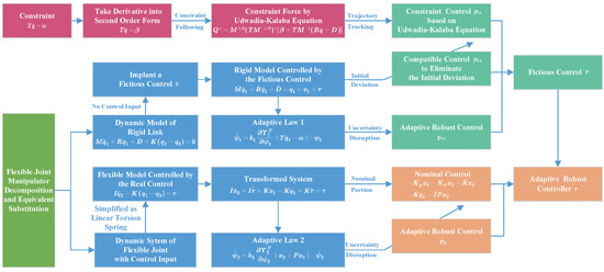
Figure 1.
Process of the control design.
Step 1. Decomposing the FJM into rigid link and flexible joint, simplify the flexibility of FJM as linear torsion spring, and get the dynamic model of the FJM system.
Step 2. Implant a fictious control into the rigid part and rewrite the dynamic model.
Step 3. Transform the constraint equation into second order differential form, and get the constraint control by UKFE equation.
Step 4. Get the compatible control based on the initial deviation to the desired trajectory.
Step 5. Design the adaptive law 1 to deal with uncertainty in rigid part, on this basis, get the adaptive robust control .
Step 6. Get the fictious control by adding , and .
Step 7. Design the nominal control for the flexible part.
Step 8. Design the adaptive law 2 to deal with the flexible joint subsystem. On this basis, get the adaptive robust control .
Step 9. Get the final controller by adding , , and the nominal control.
5. Simulations and Discussion
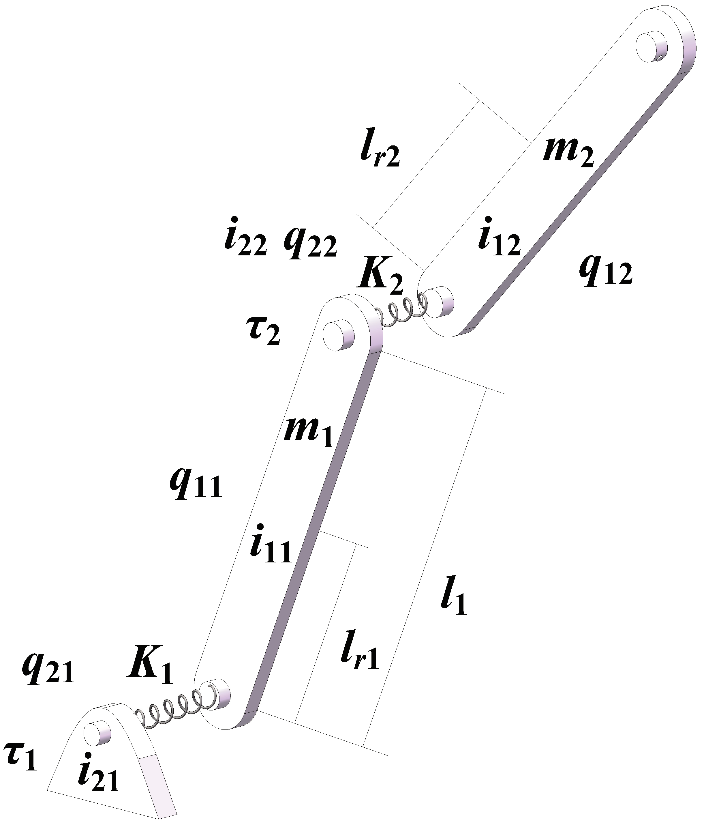
We consider a 2-link flexible joint manipulator (shown in Figure 2) to show the validity of the control proposed in this article.
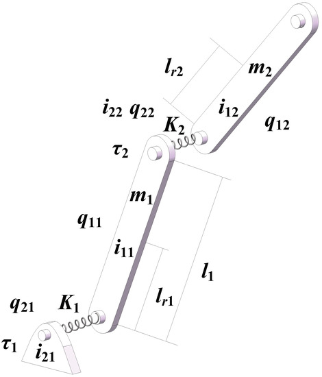
Figure 2.
2-link flexible joint manipulator.
Define the link angle vector , the joint angle vector , are the mass of links; is the length of the first link, are the centroid of the links (suppose the mass is uniformly distributed on the link), and are the moment of inertia of link and angles, respectively, denotes the torques from motors, are the stiffness of linear torsional springs; and g is the gravity coefficient. The system model is given by
where
All elements of inertia matrix are bounded by:
We require the link angles to obey the following constraints:
which means .
T is of full rank, and we notice that the desired constraints are linear with respect to velocities. Assumptions 6 and 7 are achieved by choosing
The adaptive laws are given by
We consider there exists uncertainty in and (i.e., , , , . We suppose that , . Then the simulation is performed with , , , , , , , , , , , , , . With these, we have
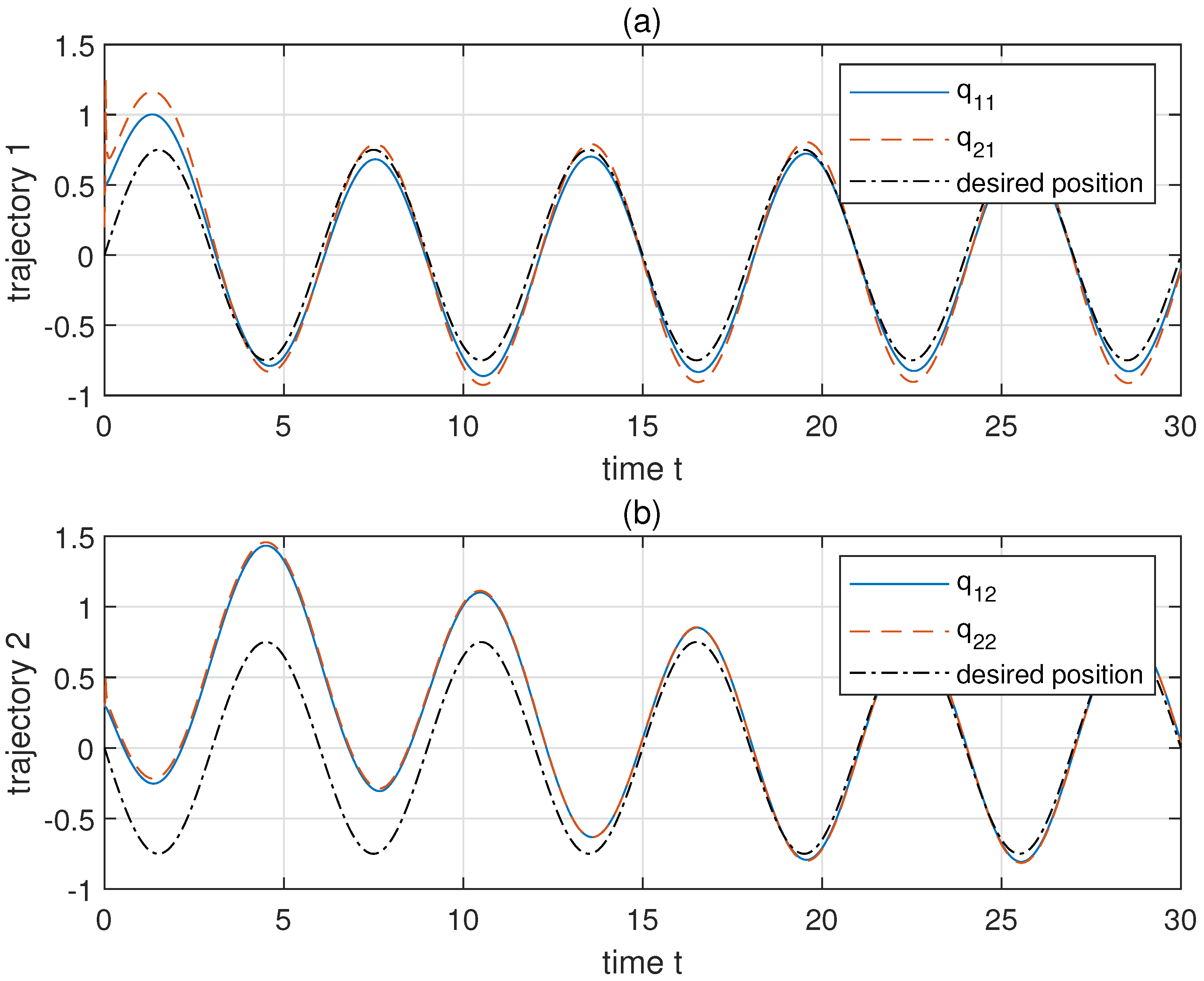
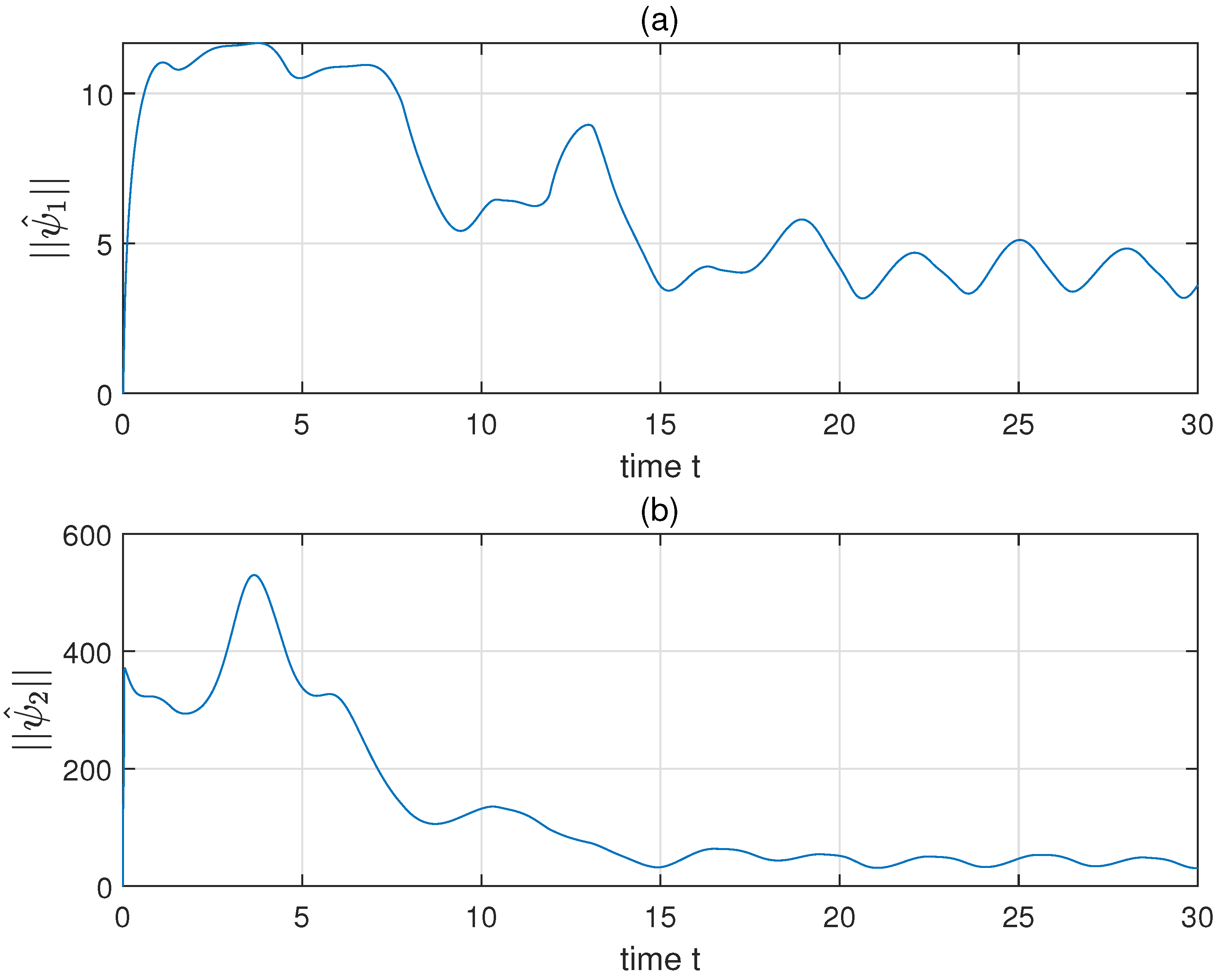
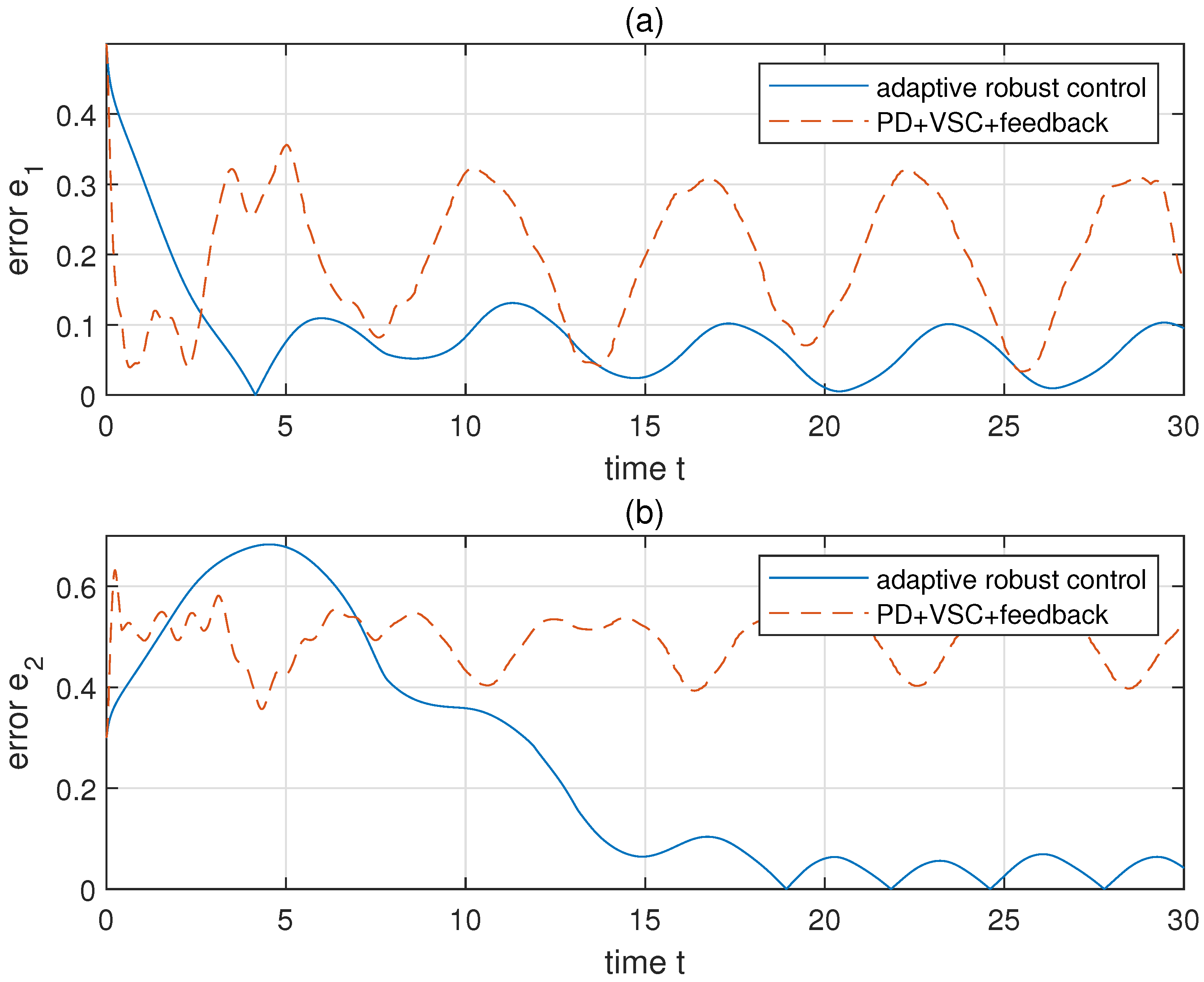
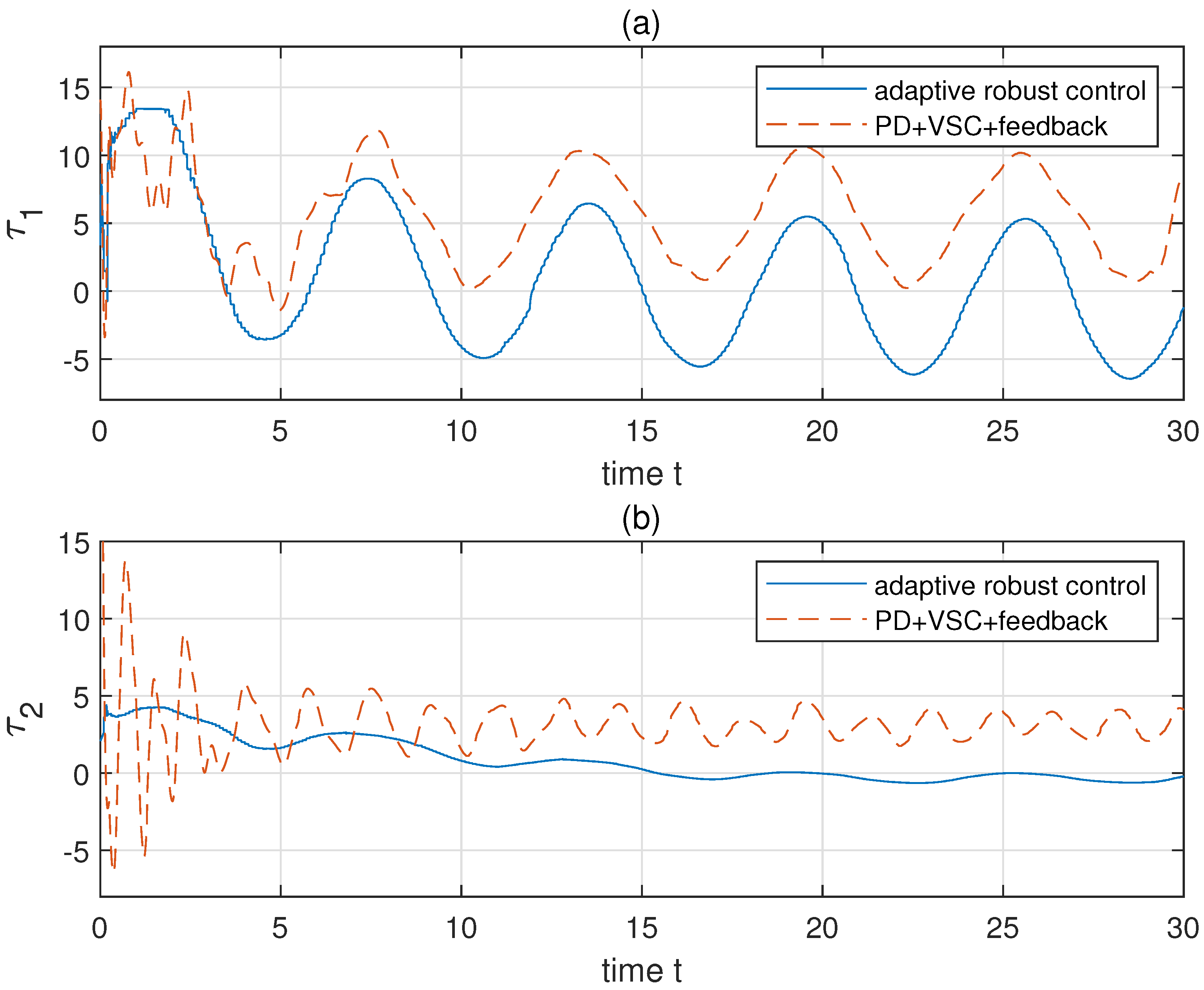
Then we choose to make ( and set . The initial , , , , , , , . For comparison, a hybrid controller, which consists of PD control, feedback control, and variable structure control (VSC), is applied to the same system with the same initial conditions and constraints [31]. Parameters of the hybrid control are chosen by: , , , , , , (details of these notations could be found in [31]). The results of simulation are shown in Figure 3, Figure 4, Figure 5, Figure 6, Figure 7 and Figure 8. Figure 3a,b shows the revolute trajectories of two links, respectively. The actual trajectories approach to the desired trajectories in a short time. This is also verified through the link position error shown in Figure 5a,b. The variation of adaptive parameters are shown in Figure 4a,b. After a local undulation, as well as converge to a region near 0. The comparison of constrained system performance by adopting the proposed adaptive robust control and a hybrid control (PD+feedback+VSC compensation) is shown in Figure 5. Obviously, the hybrid control has more unwanted waves and errors than that of the proposed control. The comparison of control torques of the two control methods is also given in Figure 6. Evidently, the hybrid control has a worse performance than the proposed adaptive robust control. The proposed control is more reposeful and its magnitude of undulation is much lower than the hybrid control.
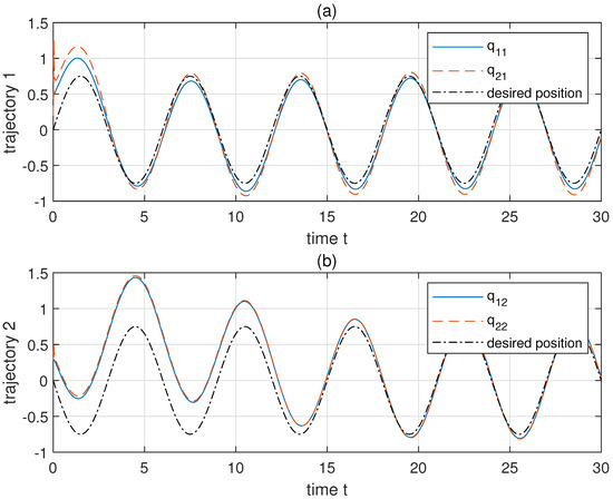
Figure 3.
The tracking performance of link position. (a,b) show the trajectories of two links, respectively.
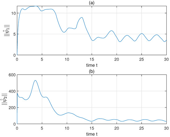
Figure 4.
The performance of system parameters. Panels (a,b) show the trend of adaptive parameters and , respectively.
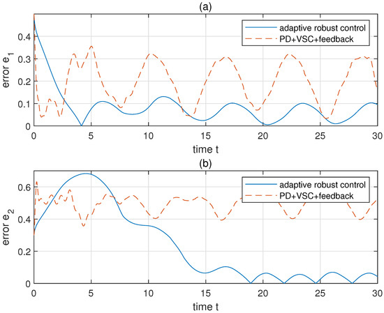
Figure 5.
The comparison of errors under adaptive robust control and PD+VSC+feedback control. Panels (a,b) show the following error and of two links, respectively.
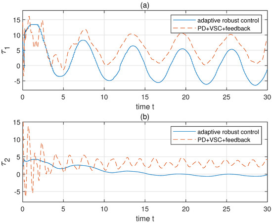
Figure 6.
The comparison of toques under adaptive robust control and PD+VSC+feedback control. Panels (a,b) show the control cost and of two links, respectively.
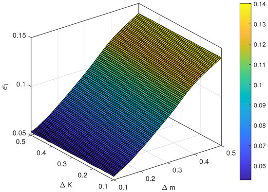
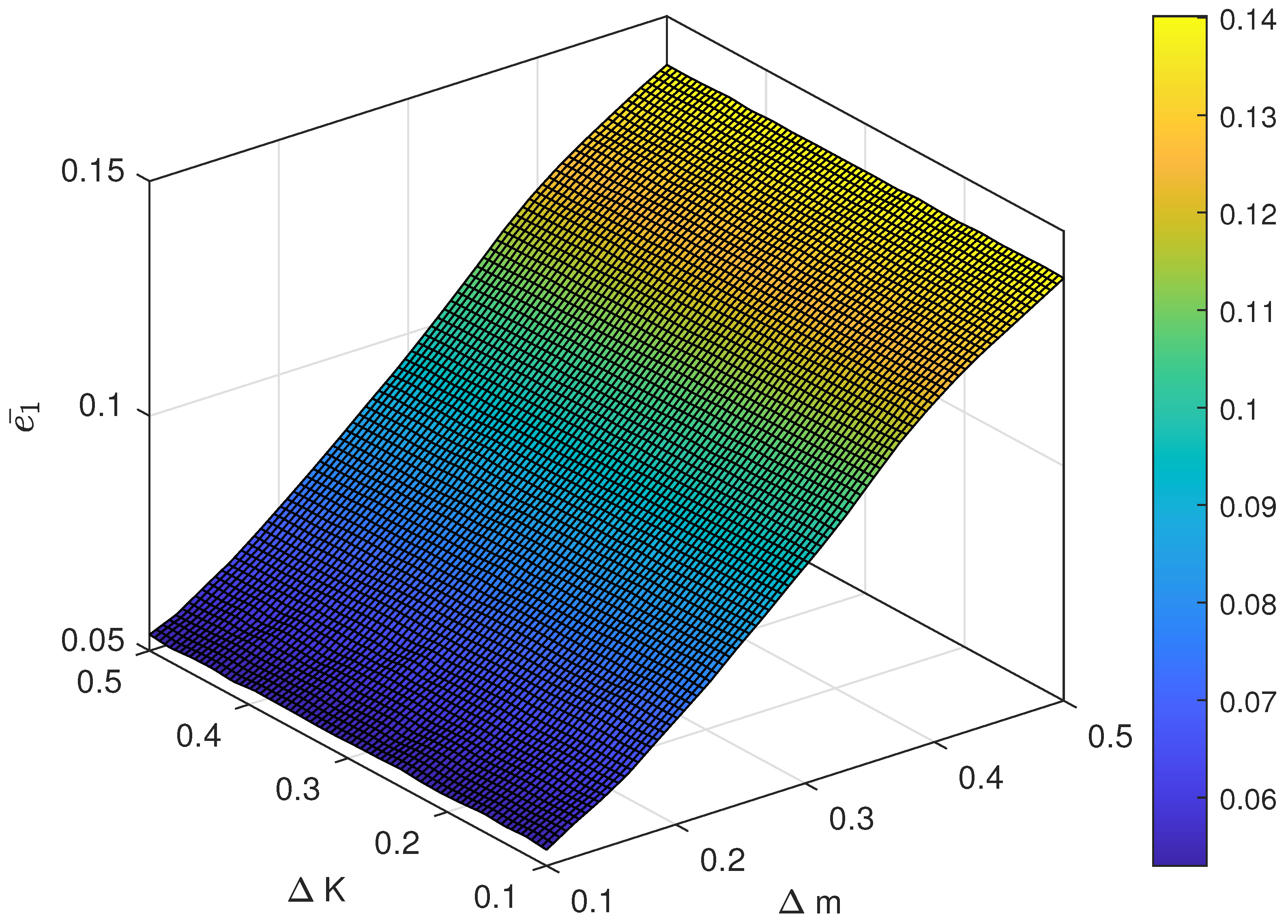
Figure 7.
The average following error under different magnitude of uncertainty.

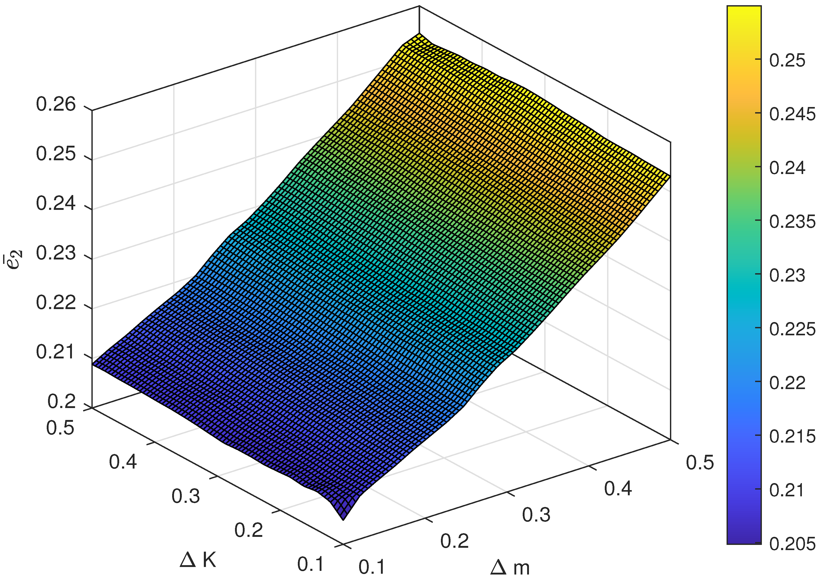
Figure 8.
The average following error under different magnitude of uncertainty.
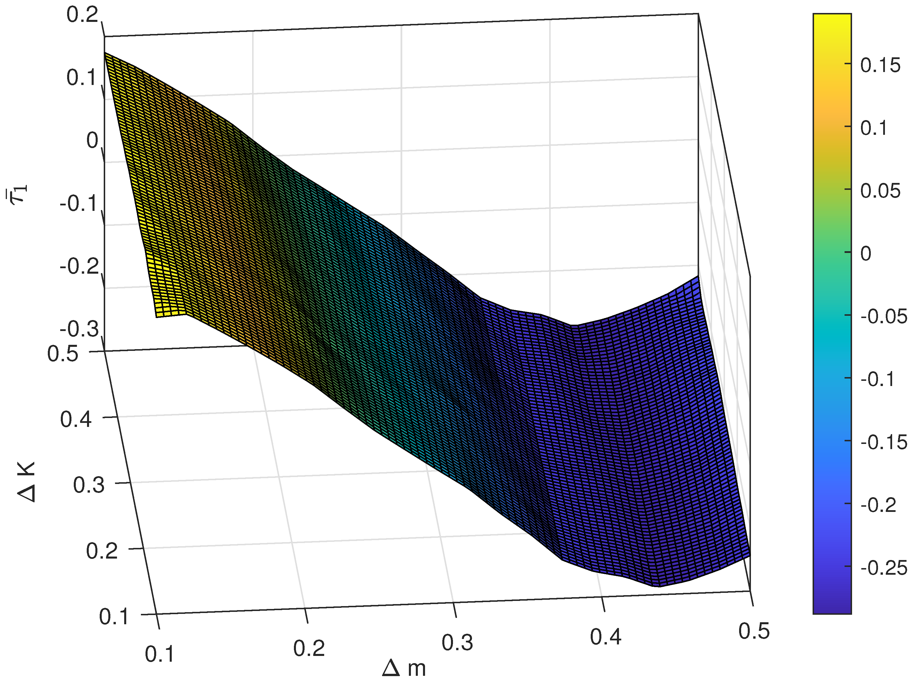
The relationship between different magnitude of uncertainty and the control performance is also investigated. For instance, the range of is chosen as , and the range of is set as . The result of the average following error and with respect to different pairs of and are shown in Figure 7 and Figure 8 and the average control cost and with respect to different pairs of and are shown in Figure 9 and Figure 10, respectively. Obviously, the proposed control has strong robustness since the average following error and the average control cost varies in a small range when the magnitude of uncertainty changes.

Figure 9.
The average control cost under different magnitude of uncertainty.
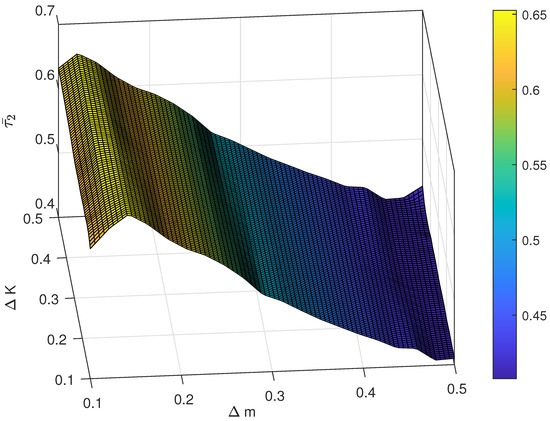
Figure 10.
The average control cost under different magnitude of uncertainty.
6. Conclusions
The constrained FJM system has strong coupling and nonlinearity. The performance would worsen when mismatched uncertainty arises. This research is on the basis of the frame built by Udwadia and Kalaba. The desired trajectory is not used to obtain the position error directly. It is treated as a constraint applied to the system and utilized to acquire the constraint force. A UKFE-based control is designed for the nominal portion of the system. No extra coordinate or Lagrange multiplier is needed other than its original ones. For the mismatched uncertainty in the system, the entire system can be divided into two cascaded subsystems by implanting a virtual control. An adaptive robust control with high-order terms is proposed to guarantee the uniform boundedness and uniform ultimate boundedness, even the information of uncertainty is poorly known. The system performance could be regulated easily by adjusting the order of the controller. Both theoretical analysis and simulation guarantees the effectiveness of the proposed control.
Author Contributions
Conceptualization, F.D.; methodology, F.D. and X.Z.; software, F.D.; investigation, X.Z.; data curation, B.Y.; writing—original draft preparation, B.Y.; writing—review and editing, H.L.; visualization, X.Z.; supervision, S.C.; project administration, F.D. All authors have read and agreed to the published version of the manuscript.
Funding
This project is supported in part by National Key R&D Program of China [Grant No. 2018YFB1308400], in part by National Natural Science Foundation of China [Grant Nos. 51905140, 61803141], in part by the University Synergy Innovation Program of Anhui Province, PR China under Grant GXXT-2019-031, and in part by the Fundamental Research Funds for the Central Universities of China [Grant Nos. PA2020GDSK0090, 300102259306].
Institutional Review Board Statement
Not applicable.
Informed Consent Statement
Not applicable.
Data Availability Statement
The data that support the findings of this study are available from the corresponding author upon reasonable request.
Conflicts of Interest
The authors declare no conflict of interest.
References
- Bottin, M.; Cocuzza, S.; Comand, N.; Doria, A. Modeling and Identification of an Industrial Robot with a Selective Modal Approach. Appl. Sci. 2020, 10, 4619. [Google Scholar] [CrossRef]
- Spong, M.W. Modeling and control of elastic joint robots. J. Dyn. Syst. Meas. Control. 1987, 109, 310–318. [Google Scholar] [CrossRef]
- Yu, Z.; Liu, X.; Cai, G. Dynamics modeling and control of a 6-DOF space robot with flexible panels for capturing a free floating target. Acta Astronaut. 2016, 128, 560–572. [Google Scholar] [CrossRef]
- Qin, H.; Li, Y.; Xiong, X. Workpiece Pose Optimization for Milling with Flexible-Joint Robots to Improve Quasi-Static Performance. Appl. Sci. 2019, 9, 1044. [Google Scholar] [CrossRef] [Green Version]
- Feng, F.; Hong, W.; Xie, L. Design of 3D-Printed Flexible Joints With Presettable Stiffness for Surgical Robots. IEEE Access 2020, 8, 79573–79585. [Google Scholar] [CrossRef]
- Zou, S.; Bo, P.; Xu, H.; Guo, S. Extended high-gain observer based adaptive control of flexible-joint surgical robot. In Proceedings of the IEEE International Conference on Robotics & Biomimetics, Qingdao, China, 3–7 December 2016; pp. 2128–2133. [Google Scholar]
- Li, X.; Pan, Y.; Chen, G.; Yu, H. Adaptive Human-Robot Interaction Control for Robots Driven by Series Elastic Actuators. IEEE Trans. Robot. 2017, 33, 169–182. [Google Scholar] [CrossRef]
- Yao, W.; Zhang, D.; Guo, Y.; Wu, Y.; Guo, J. Improved hierarchical sliding mode control for flexible-joint manipulator. J. Southeast Univ. 2018, 48, 201–206. [Google Scholar]
- Zaare, S.; Soltanpour, M.R.; Moattari, M. Adaptive sliding mode control of n flexible-joint robot manipulators in the presence of structured and unstructured uncertainties. Multibody Syst. Dyn. 2019, 47, 397–434. [Google Scholar] [CrossRef]
- He, W.; Yan, Z.; Sun, Y.; Ou, Y.; Sun, C. Neural-Learning-Based Control for a Constrained Robotic Manipulator With Flexible Joints. IEEE Trans. Neural Netw. Learn. Syst. 2018, 29, 5993–6003. [Google Scholar] [CrossRef]
- Chu, M.; Jia, Q.; Sun, H. Backstepping Control for Flexible Joint with Friction Using Wavelet Neural Networks and L-2-Gain Approach. Asian J. Control 2018, 20, 856–866. [Google Scholar] [CrossRef]
- Liu, Z.; Liu, J. Boundary Control of a Flexible Robotic Manipulator With Output Constraints. Asian J. Control 2017, 19, 332–345. [Google Scholar] [CrossRef]
- Kelekci, E.; Kizir, S. Trajectory and vibration control of a flexible joint manipulator using interval type-2 fuzzy logic. ISA Trans. 2019, 94, 218–233. [Google Scholar] [CrossRef]
- Sun, W.; Su, S.; Xia, J.; Nguyen, V.T. Adaptive Fuzzy Tracking Control of Flexible-Joint Robots With Full-State Constraints. IEEE Trans. Syst. Man Cybern. Syst. 2019, 49, 2201–2209. [Google Scholar] [CrossRef]
- Ulrich, S.; Sasiadek, J. On the Simple Adaptive Control of Flexible-Joint Space Manipulators with Uncertainties. Annu. Rev. Earth Planet. Sci. 2015, 24, 13–23. [Google Scholar]
- Ibrahim, K.; Sharkawy, A. A hybrid PID control scheme for flexible joint manipulators and a comparison with sliding mode control. Ain Shams Eng. J. 2018, 9, 3451–3457. [Google Scholar] [CrossRef]
- Chen, Y.H. Constraint-following Servo Control Design for Mechanical Systems. J. Vib. Control 2009, 15, 369–389. [Google Scholar] [CrossRef]
- Udwadia, F.E.; Kalaba, R.E. A New Perspective on Constrained Motion. Proc. R. Soc. Lond. Ser. A Math. Phys. Sci. 1992, 439, 407–410. [Google Scholar]
- Udwadia, F.E.; Kalaba, R.E. On motion. J. Frankl. Inst. 1993, 330, 571–577. [Google Scholar] [CrossRef]
- Chen, Y.H. Equations of motion of constrained mechanical systems: Given force depends on constraint force. Mechatronics 1999, 9, 411–428. [Google Scholar] [CrossRef]
- Chen, Y.H. Second-order constraints for equations of motion of constrained systems. Mechatron. IEEE/ASME Trans. 1998, 3, 240–248. [Google Scholar] [CrossRef]
- Chen, Y.H. Equations of motion of mechanical systems under servo constraints: The Maggi approach. Mechatronics 2008, 18, 208–217. [Google Scholar] [CrossRef]
- Xu, J.; Chen, Y.H.; Guo, H. A New Approach to Control Design for Constraint-following for Fuzzy Mechanical Systems. J. Optim. Theory Appl. 2015, 165, 1022–1049. [Google Scholar] [CrossRef]
- Zhao, X.; Chen, Y.H.; Zhao, H.; Dong, F. Control Design for Artificial Swarm Mechanical Systems: Dynamics, Uncertainty, and Constraint. Asian J. Control 2018, 20, 2042–2050. [Google Scholar] [CrossRef]
- Zhao, X.; Chen, Y.H.; Dong, F.; Zhao, H. Controlling Uncertain Swarm Mechanical Systems: A β-Measure Based Approach. IEEE Trans. Fuzzy Syst. 2019, 27, 1272–1285. [Google Scholar] [CrossRef]
- Zhao, R.; Chen, Y.H.; Jiao, S.; Ma, X. A constraint-following control for uncertain mechanical systems: Given force coupled with constraint force. Nonlinear Dyn. 2018, 93, 1201–1217. [Google Scholar] [CrossRef]
- Xu, J.; Fang, H.; Chen, Y.H.; Guo, H.; Ding, X. Guaranteeing performance for uncertain nonlinear systems with bounded state constraint and mismatching condition. Asian J. Control 2019, 23, 548–560. [Google Scholar] [CrossRef]
- Chen, Y.H.; Leitmann, G.; Chen, J.S. Robust control for rigid serial manipulators: A general setting. In Proceedings of the 1998 American Control Conference, Philadelphia, PA, USA, 26 June 1998; Volume 2, pp. 912–916. [Google Scholar]
- Udwadia, F.E.; Kalaba, R.E. Analytical Dynamics: A New Approach; Cambridge University Press: Cambridge, UK, 1996. [Google Scholar]
- Wu, L.; Zhao, R.; Li, Y.; Chen, Y.H. Optimal Design of Adaptive Robust Control for the Delta Robot with Uncertainty: Fuzzy Set-Based Approach. Appl. Sci. 2020, 10, 3472. [Google Scholar] [CrossRef]
- Tang, J.; Ouyang, P.; Yue, W.; Kang, H. Nonlinear PD sliding mode control for robotic manipulator. In Proceedings of the 2017 IEEE International Conference on Advanced Intelligent Mechatronics (AIM), Munich, Germany, 3–7 July 2017; pp. 1004–1008. [Google Scholar] [CrossRef]


Publisher’s Note: MDPI stays neutral with regard to jurisdictional claims in published maps and institutional affiliations. |
© 2021 by the authors. Licensee MDPI, Basel, Switzerland. This article is an open access article distributed under the terms and conditions of the Creative Commons Attribution (CC BY) license (https://creativecommons.org/licenses/by/4.0/).