
Modelling and Stability Analysis for a Magnetically Levitated Slice Motor (MLSM) with Gyroscopic Effect and Non-Collocated Structure Based on the Extended Inverse Nyquist Stability Criterion


Abstract
:1. Introduction
2. Modelling of MLSM with Gyroscopic Effect and Non-Collocated Structure
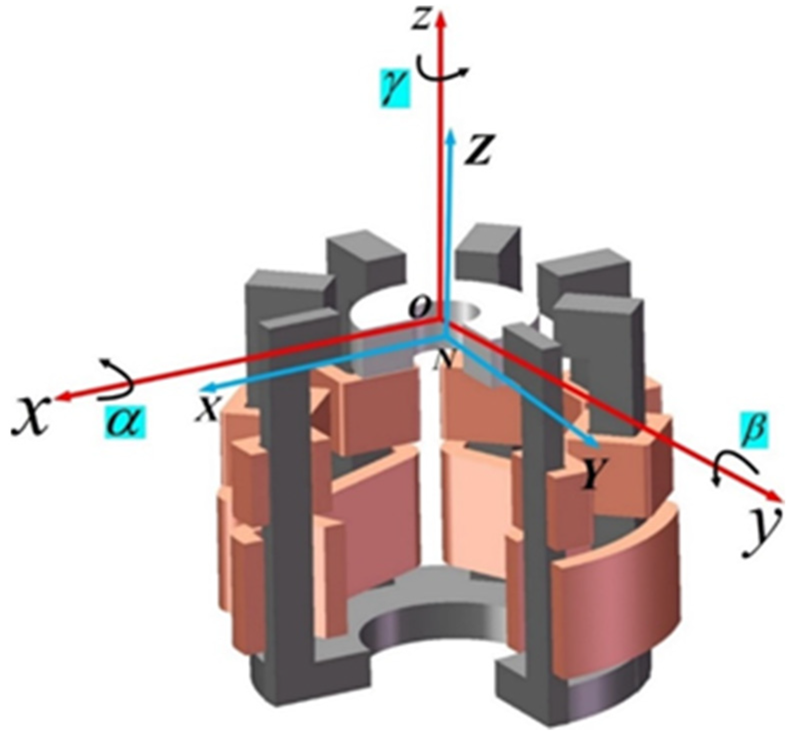
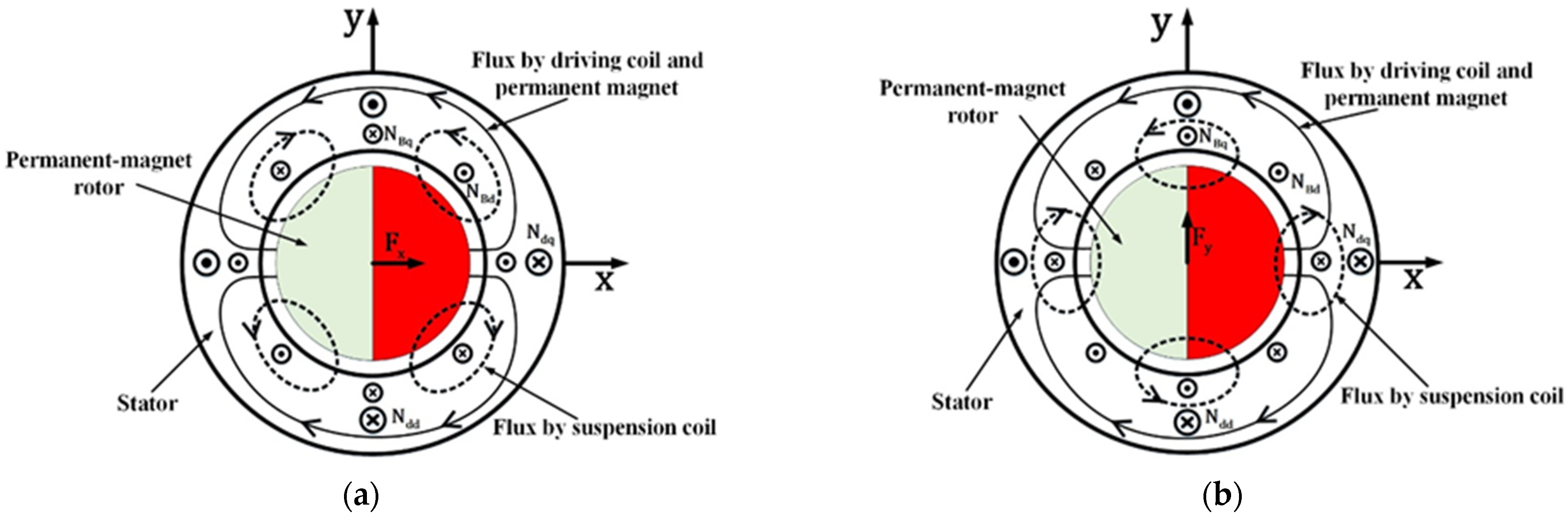
2.1. Working Principle of the MLSM
2.2. Kinetics Analysis of the MLSM System Featured with Gyroscopic Effect
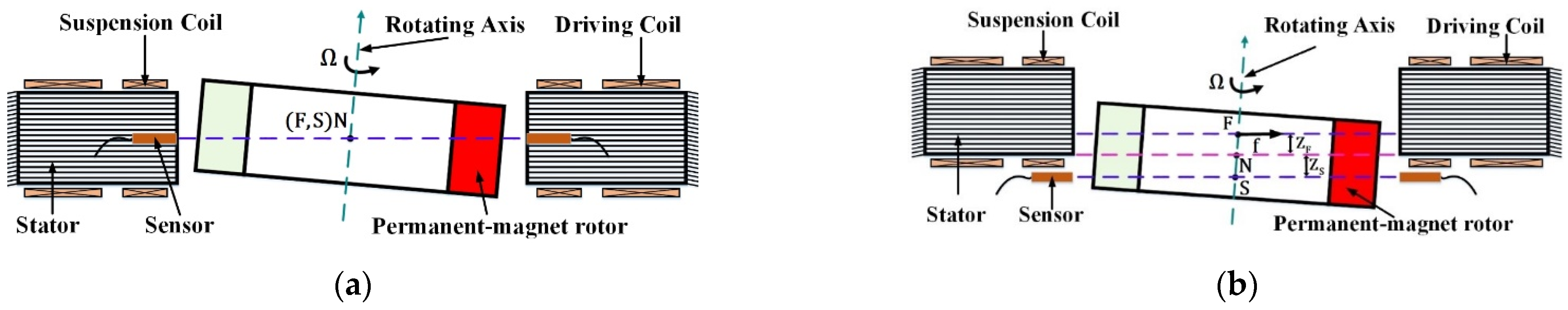
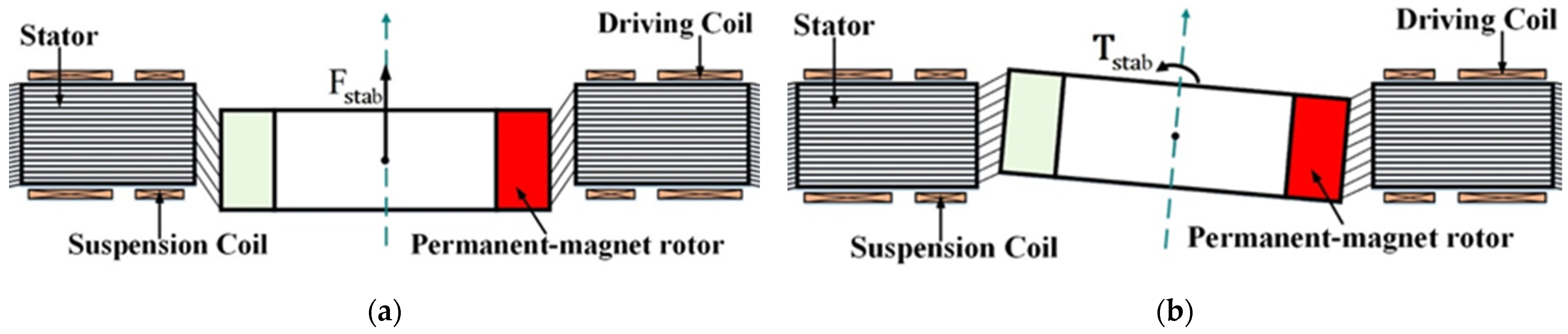
2.3. Description of the MLSM with Non-Collocated Structure
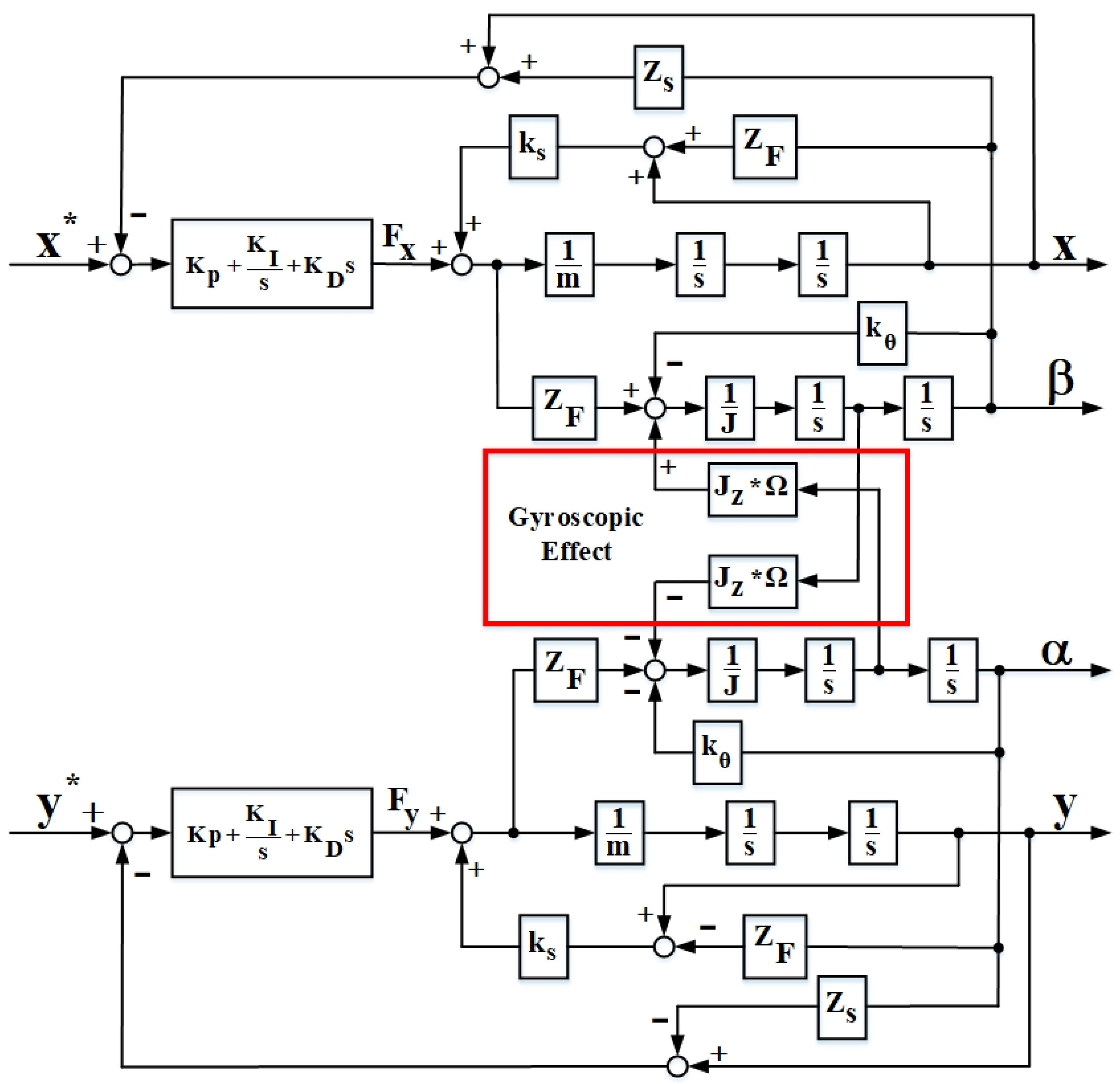
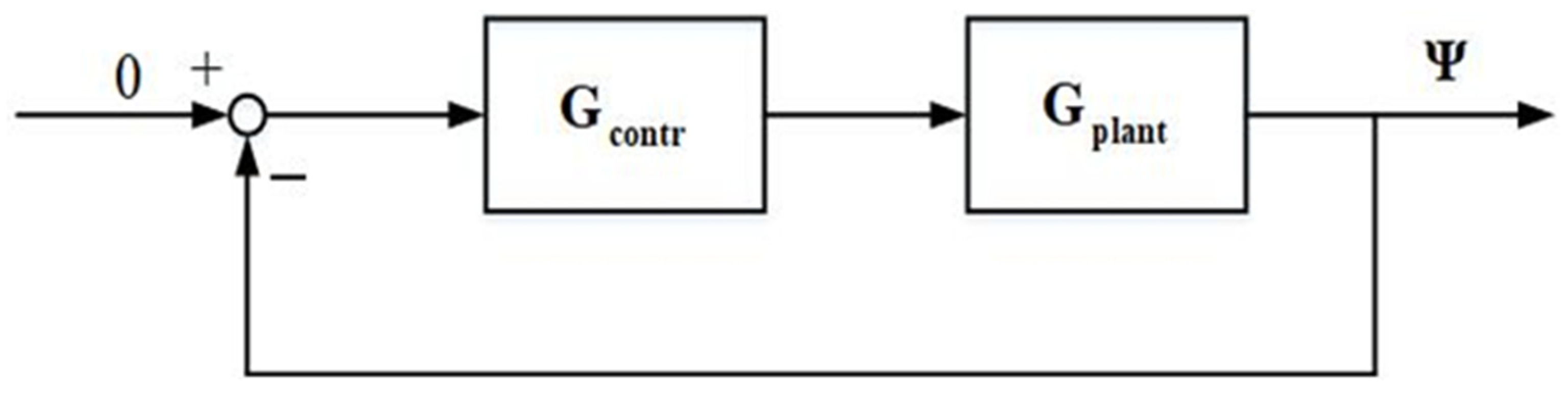
2.4. Analytical Model of the Controlled MLSM System with Gyroscopic Effect and Non-Collocated Structure
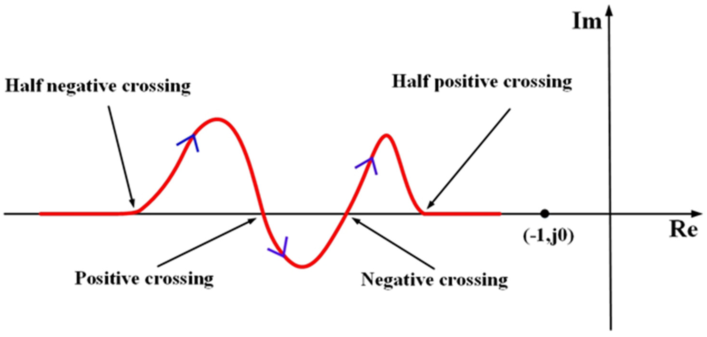
3. Extended Inverse Nyquist Stability Criterion in the Complex Domain
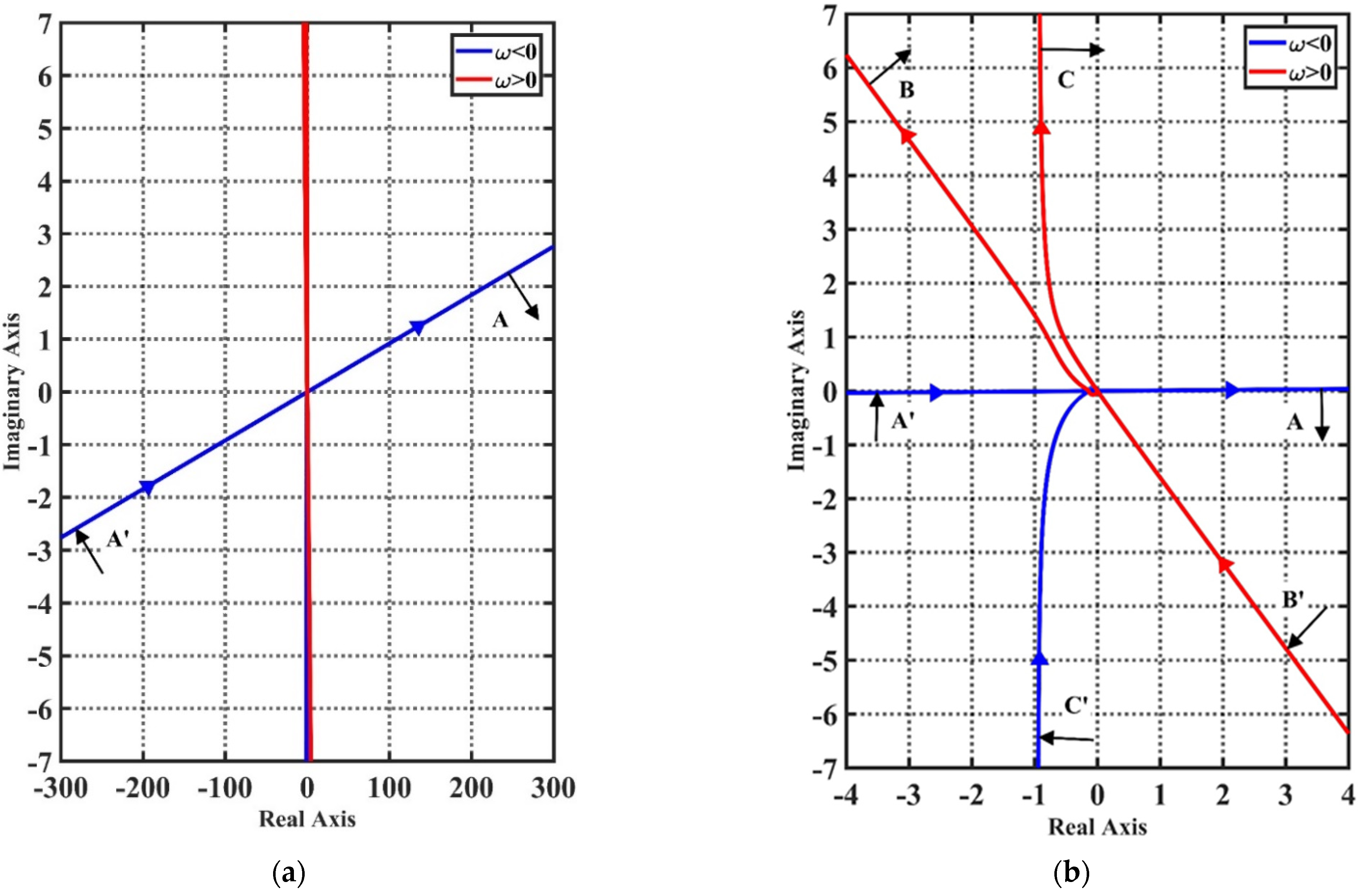
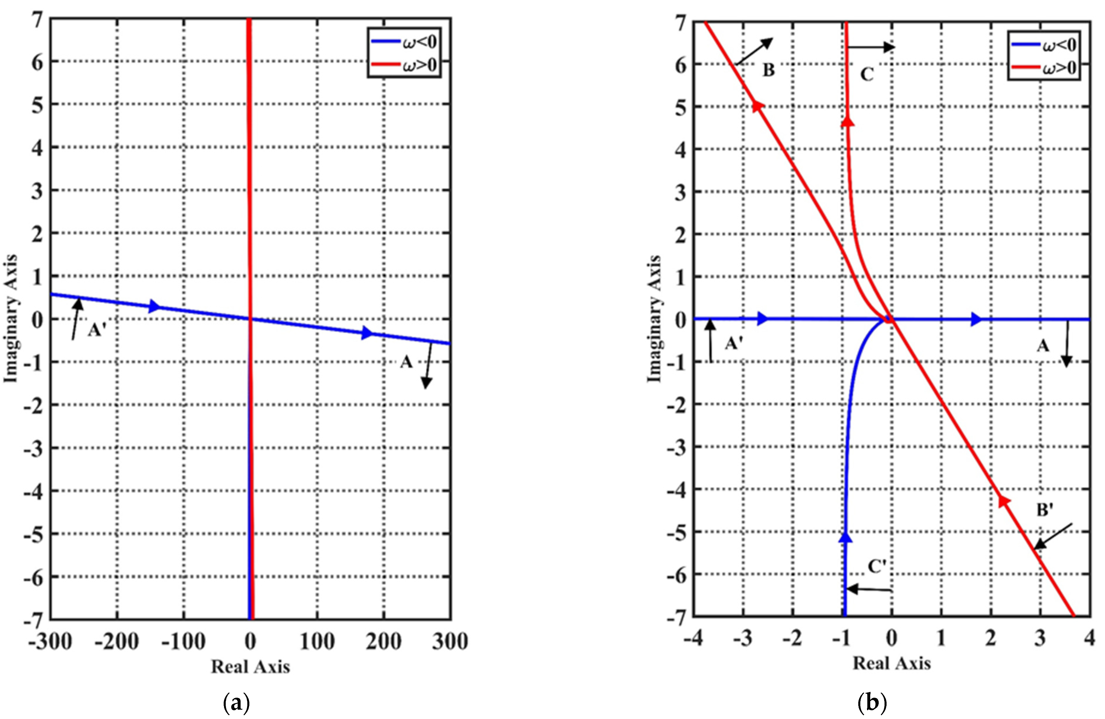
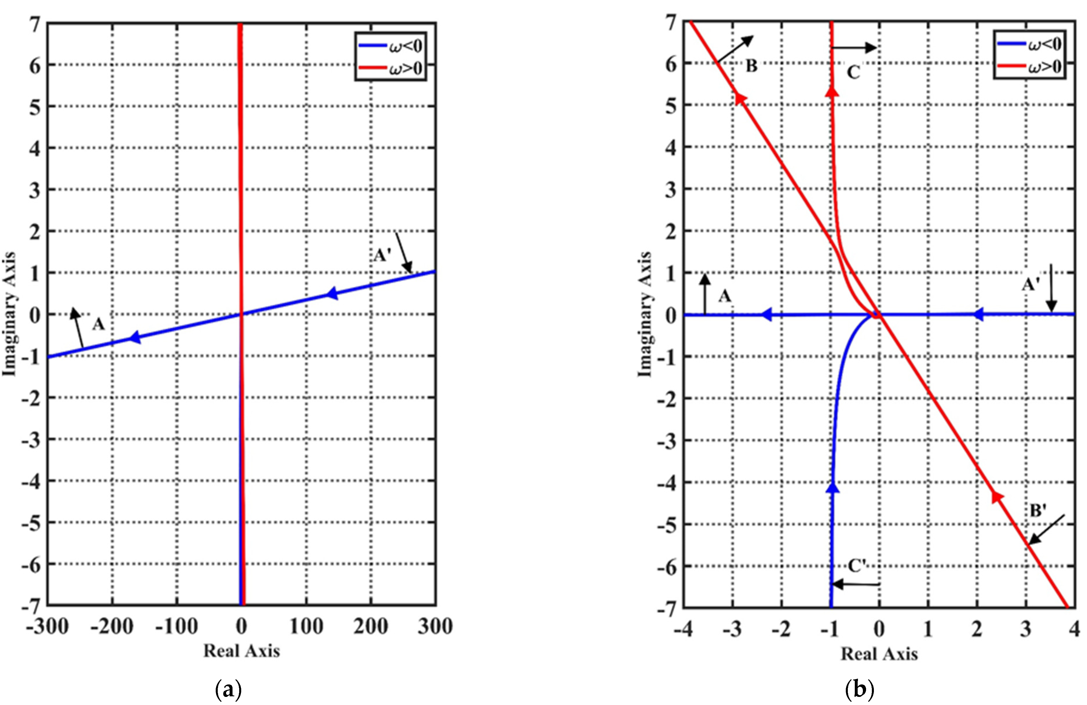
4. Stability Analysis on MLSM with Gyroscopic Effect and Non-Collocated Structure
- (1)
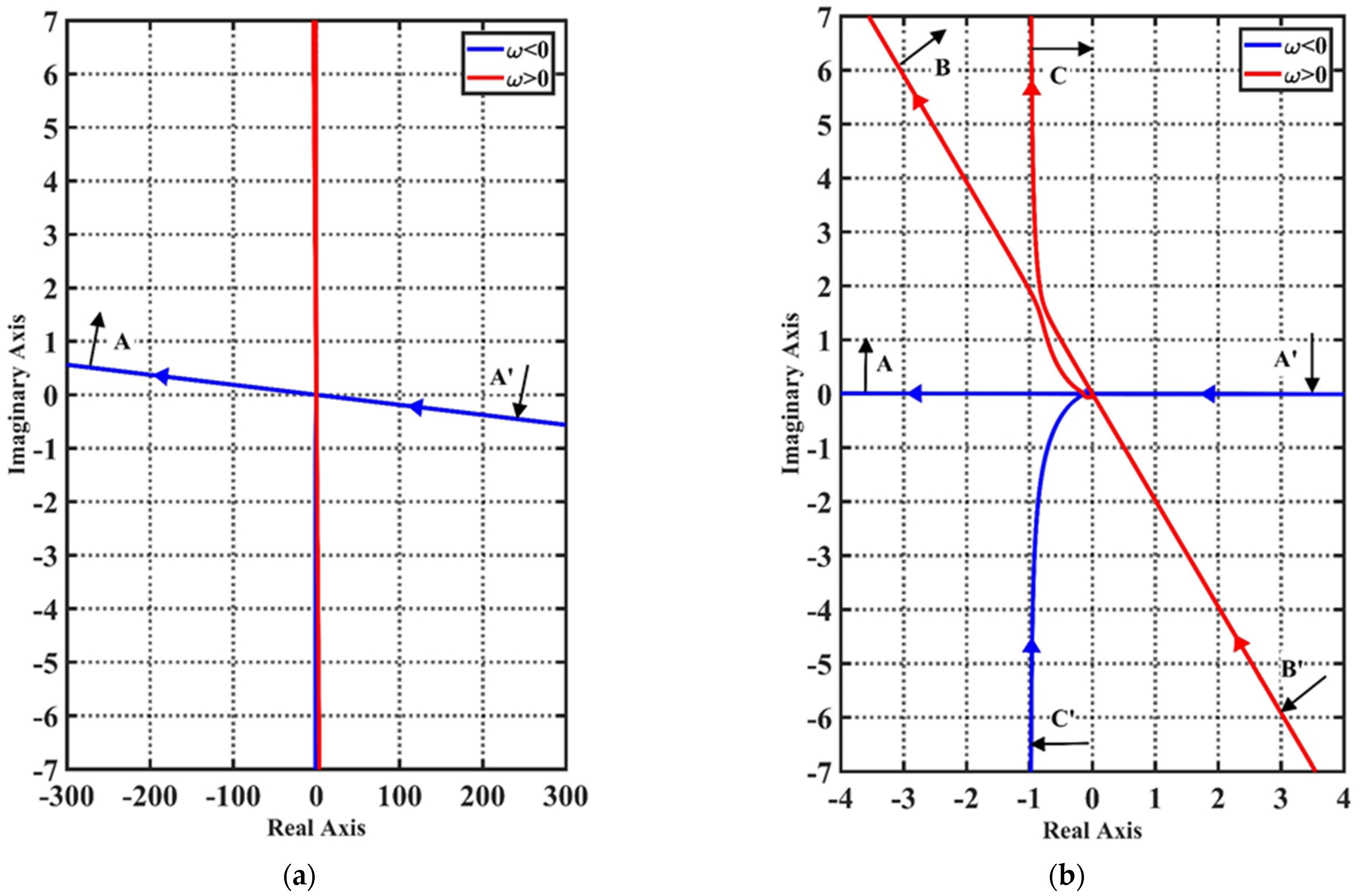
- When , the sufficient and necessary condition for the absolute stability is that the inverse Nyquist curve of the open-loop transfer function encloses counterclockwise once.
- (2)
- When , the sufficient and necessary condition for the absolute stability is that the inverse Nyquist curve of the open-loop transfer function encircles zero times.
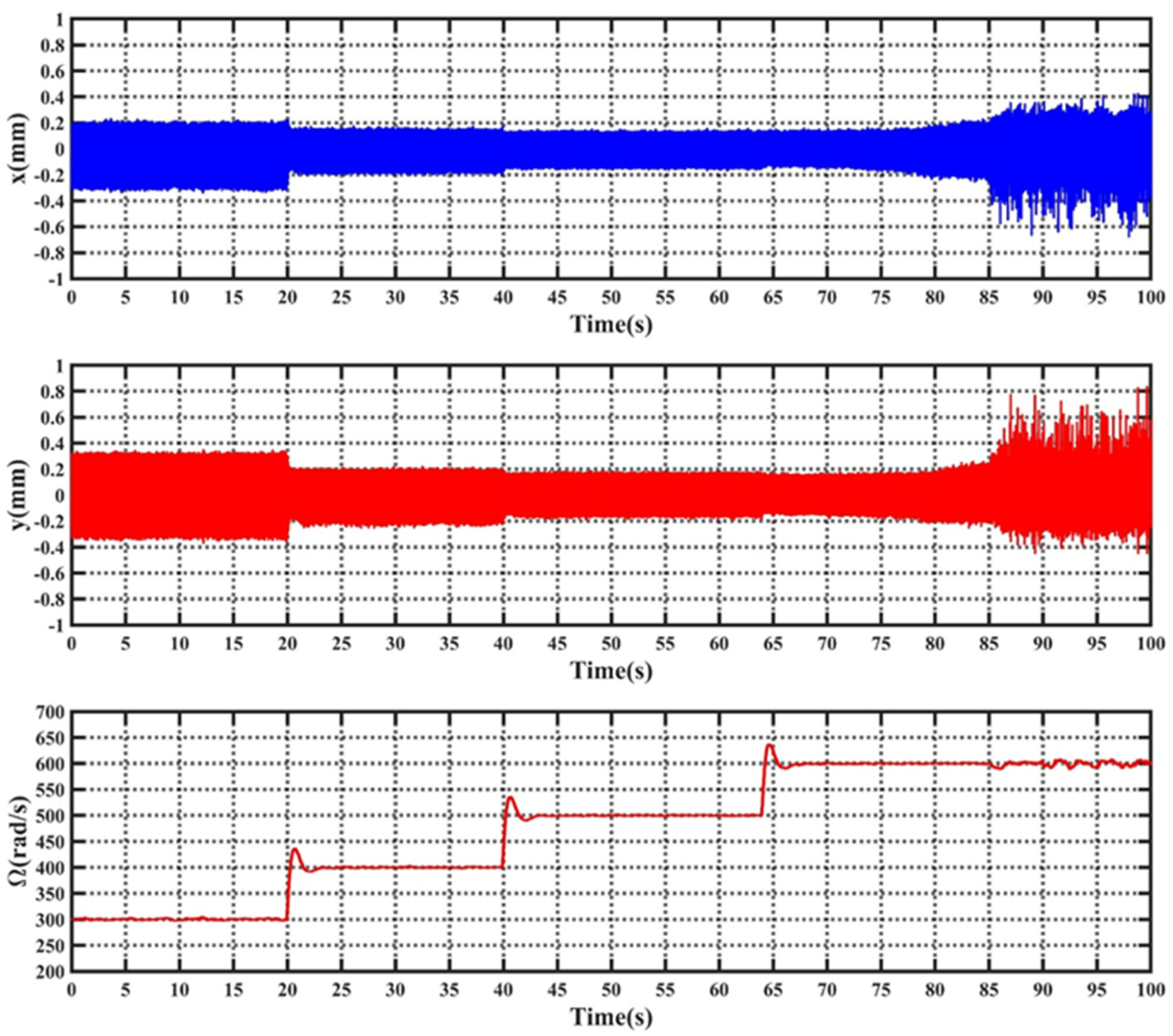
5. Simulation and Experimental Results
6. Conclusions
Author Contributions
Funding
Conflicts of Interest
Nomenclature
| MLSM | Magnetically levitated slice motor. |
| MIMO | Multiple-input and multiple-output. |
| SISO | Single-input and single-out. |
| Suspension coils and driving coils. | |
| Inclinations of rotor about x-, y-, and z-axes. | |
| Spin velocity. | |
| Mass of the rotor. | |
| Moment of inertia of the rotor about Z-axis. | |
| Moment of inertia of the rotor about X- and Y-axes. | |
| Radial stiffness in x-and y-directions. | |
| Tilting stiffness in x-and y-directions. | |
| , | Total disturbance forces in -and -directions. |
| Total disturbance moments in -and -directions. | |
| Axial position of radial displacement sensors. | |
| Equivalent application point of radial suspension force. | |
| Center of gravity of rotor. | |
| Distance of S with respect to N. | |
| Distance of F with respect to N. | |
| Parameters of the radial translational controllers. |
References
- Warberger, B.; Kaelin, R.; Nussbaumer, T.; Kolar, J.W. 50-/2500-W Bearingless Motor for High-Purity Pharmaceutical Mixing. IEEE Trans. Ind. Electron. 2012, 59, 2236–2247. [Google Scholar] [CrossRef]
- Li, Q.N.; Boesch, P.; Haefliger, M.; Kolar, J.W.; Xu, D.H. Basic characteristics of a 4kW permanent-magnet type bearingless slice motor for centrifugal pump system. In Proceedings of the 2008 International Conference on Electrical Machines and Systems, Wuhan, China, 17–20 October 2008; pp. 3037–3042. [Google Scholar]
- Press Release IBM. Chartered, Infineon and Samsung Announce Process and Design Readiness for Silicon Circuits on 45 nm Low-Power Technology. Available online: https://www.design-reuse.com/news/14108/ibm-chartered-infineon-samsung-process-design-readiness-silicon-circuits-45nm-power-technology.html (accessed on 13 September 2021).
- Neff, M.; Barletta, N.; Schöb, R. Bearingless Centrifugal Pump for Highly Pure Chemicals. In Proceedings of the 8th International Symposium on Magnetic Bearing, Mito, Japan, 26–28 August 2002. [Google Scholar]
- Bu, W.S.; Huang, S.H.; Wan, S.M.; Liu, W.S. General Analytical Models of Inductance Matrices of Four-Pole Bearingless Motors with Two-Pole Controlling Windings. IEEE Trans. Magn. 2009, 45, 3316–3321. [Google Scholar] [CrossRef]
- Weinreb, B.S. A novel Magnetically Levitated Interior Permanent Magnet Slice Motor. Master′s Thesis, Massachusetts Institute of Technology, Cambridge, MA, USA, 2020. [Google Scholar]
- Zhang, S.R.; Fang, L.L. Direct Control of Radial Displacement for Bearingless Permanent-Magnet-Type Synchronous Motors. IEEE Trans. Ind. Electron. 2009, 56, 542–552. [Google Scholar] [CrossRef]
- Mitterhofer, H. Towards High-Speed Bearingless Disk Drives. Ph.D. Thesis, Johannes Kepler University Linz, Linz, Austria, 2017. [Google Scholar]
- Ahrens, M.; Kucera, L.; Larsonneur, R. Performance of a magnetically suspended flywheel energy storage device. IEEE Trans. Control Syst. Technol. 1996, 4, 494–502. [Google Scholar] [CrossRef]
- Sun, M.L.; Zheng, S.Q.; Wang, K.; Le, Y. Filter Cross-Feedback Control for Nutation Mode of Asymmetric Rotors with Gyroscopic Effects. IEEE ASME Trans. Mechatron. 2020, 25, 248–258. [Google Scholar] [CrossRef]
- Ahrens, M.; Kucera, L. Cross Feedback Control of a Magnetic Bearing System: Controller Design Considering Gyroscopic Effects. In Proceedings of the 3th International Symposium on Magnetic Suspension Technology, Tallahassee, FL, USA, 13–15 December 1995. [Google Scholar]
- Karutz, P.; Nussbaumer, T.; Gruber, W.; Kolar, J.W. Novel Magnetically Levitated Two-Level Motor. IEEE ASME Trans Mechatron. 2008, 13, 658–668. [Google Scholar] [CrossRef]
- Masuzawa, T.; Kita, T.; Okada, Y. An ultradurable and compact rotary blood pump with a magnetically suspended impeller in the radial direction. Artif. Organs 2015, 25, 395–399. [Google Scholar] [CrossRef] [PubMed]
- Bartholet, M.T.; Nussbaumer, T.; Silber, S.; Kolar, J.W. Comparative Evaluation of Polyphase Bearingless Slice Motors for Fluid-Handling Applications. IEEE Trans. Ind. Appl. 2009, 45, 1821–1830. [Google Scholar] [CrossRef]
- Sugimoto, H.; Chiba, A. Stability Consideration of Magnetic Suspension in Two-Axis Actively Positioned Bearingless Motor with Collocation Problem. IEEE Trans. Ind. Appl. 2014, 50, 338–345. [Google Scholar] [CrossRef]
- Tang, J.Q.; Zhao, S.P.; Wang, Y.; Wang, K. High-speed Rotor’s Mechanical Design and Stable Suspension Based on Inertia-ratio for Gyroscopic Effect Suppression. Int. J. Control Autom. 2018, 16, 1577–1591. [Google Scholar] [CrossRef]
- Schweitze, G.; Maslen, E. Magnetic Bearings-Theory, Design, and Application to Rotating Machinery; Springer: Berlin/Heidelberg, Germany, 2009; pp. 168–179. [Google Scholar]
- Fang, J.C.; Ren, Y.; Fan, Y.H. Nutation and Precession Stability Criterion of Magnetically Suspended Rigid Rotors with Gyroscopic Effects Based on Positive and Negative Frequency Characteristics. IEEE Trans. Ind. Electron. 2013, 61, 2003–2014. [Google Scholar] [CrossRef]
- Wei, J.B.; Liu, K.; Radice, G. Study on stability and rotating speed stable region of magnetically suspended rigid rotors using extended Nyquist criterion and gain-stable region theory. ISA Trans. 2016, 66, 154–163. [Google Scholar] [CrossRef] [PubMed] [Green Version]
- Sugimoto, H.; Shimura, I.; Chiba, A. A novel simplified structure for single-drive bearingless motor. In Proceedings of the 2016 IEEE Energy Conversion Congress and Exposition (ECCE), Milwaukee, WI, USA, 18–22 September 2016; pp. 1–7. [Google Scholar] [CrossRef]
- Sugimoto, H.; Chiba, A. Experimental Results Passing Through Critical Speeds of Radial and Tilting Motions in a One-Axis Actively Positioned Single-Drive Bearingless Motor. In Proceedings of the 2018 IEEE Energy Conversion Congress and Exposition (ECCE), Portland, OR, USA, 23–27 September 2018; pp. 4392–4397. [Google Scholar] [CrossRef]
- Sugimoto, H.; Miyoshi, M.; Chiba, A. Low speed test in two-axis actively positioned bearingless machines with non-collocated structure for wind power applications. In Proceedings of the 2015 IEEE Energy Conversion Congress and Exposition (ECCE), Montreal, QC, Canada, 20–24 September 2015; pp. 799–804. [Google Scholar] [CrossRef]
- Sun, X.D.; Chen, L.; Yang, Z.B. Overview of Bearingless Permanent-Magnet Synchronous Motors. IEEE Trans. Ind. Electron. 2013, 60, 5528–5538. [Google Scholar] [CrossRef]
- Raggl, K.; Kolar, J.W. Comparison of Winding Concepts for Bearingless Pumps. In Proceedings of the 7th International Conference on Power Electronics, Daegu, Korea, 22–26 October 2007; pp. 1013–1020. [Google Scholar] [CrossRef]
- Ooshima, M.; Chiba, A.; Fukao, T. Design and Analysis of Permanent Magnet-Type Bearingless Motors. IEEE Trans. Ind. Electron. 1996, 43, 292–299. [Google Scholar] [CrossRef]
- Mamat, N.; Karim, K.A.; Ibrahim, Z. Bearingless Permanent Magnet Synchronous Motor using Independent Control. Int. J. Power Electron. Drive Syst. 2015, 6, 233–241. [Google Scholar] [CrossRef]
- Zhang, W.; Zhu, H.Q.; Xu, Y.; Wu, M.Y. Direct Control of Bearingless Permanent Magnet Slice Motor Based on Active Disturbance Rejection Control. IEEE Trans. Appl. Supercon. 2020, 30, 1–5. [Google Scholar] [CrossRef]
- Mitterhofer, M.; Amrhein, W. Design aspects and test results of a high speed bearingless drive. In Proceedings of the 2011 IEEE Ninth International Conference on Power Electronics and Drive Systems, Singapore, 5–8 December 2011; pp. 705–710. [Google Scholar] [CrossRef]
- Zhu, H.Q.; Li, F.Y. Optimization Design of Bearingless Permanent-Magnet Slice Motor. IEEE Trans. Appl. Supercon. 2016, 26, 1–4. [Google Scholar] [CrossRef]
- Michioka, C.; Sakamoto, T.; Ichikawa, O.; Chiba, A.; Fukao, T. A decoupling control method of reluctance-type bearingless motors considering magnetic saturation. IEEE Trans. Ind. Appl. 1996, 32, 1204–1210. [Google Scholar] [CrossRef]
- Bouzidi, R.; Van, A.L. Lagrangian Mechanics: An Advanced Analytical Approach; Wiley-ISTE: Hoboken, NJ, USA; London, UK, 2019; pp. 111–129. [Google Scholar]
- Bösch, P.N. Lagerlose Scheibenläufermotoren höherer Leistung. Ph.D. Thesis, ETH Zurich, Zurich, Switzerland, 2004. [Google Scholar]
- Liu, C.; Liu, G. Equivalent Damping Control of Radial Twist Motion for Permanent Magnetic Bearings Based on Radial Position Variation. IEEE Trans. Ind. Electron. 2015, 62, 6417–6427. [Google Scholar] [CrossRef]
- Troeng, O.; Bernhardsson, B.; Rivetta, C. Complex-coefficient systems in control. In Proceedings of the 2017 American Control Conference (ACC), Seattle, WA, USA, 24–26 May 2017; pp. 1721–1727. [Google Scholar] [CrossRef] [Green Version]
- Zhang, S.C.; Xia, Y.S. Solving Nonlinear Optimization Problems of Real Functions in Complex Variables by Complex-Valued Iterative Methods. IEEE Trans. Cybern. 2018, 48, 277–287. [Google Scholar] [CrossRef]
- Ahlfors, L. Complex Analysis; McGraw-Hill: New York, NY, USA, 1979. [Google Scholar]
- Garcia-Sanz, M. The Nyquist stability criterion in the Nichols chart. Int. J. Robust Nonlinear Control 2016, 26, 2643–2651. [Google Scholar] [CrossRef]
- Fang, B. Computation of stabilizing PID gain regions based on the inverse Nyquist plot. J. Process Control 2010, 20, 1183–1187. [Google Scholar] [CrossRef]
- Wen, B.; Boroyevich, D.; Burgos, R. Inverse Nyquist Stability Criterion for Grid-Tied Inverters. IEEE Trans. Power Electron. 2016, 32, 1548–1556. [Google Scholar] [CrossRef]
- Ogata, K. Modern Control Engineering, 5th ed.; Prentice-Hall: Englewood Cliffs, NJ, USA, 2010; pp. 398–462. [Google Scholar]
- Oppenheim, A.V.; Nawab, S.H.; Willsky, A.S. Signals and Systems, 2nd ed.; Prentice-Hall: Englewood Cliffs, NJ, USA, 1997; pp. 461–485. [Google Scholar]


| Condition | Characteristic of the Inverse Nyquist Plot | |
|---|---|---|
| Symmetry about the imaginary axis | Turn clockwise from to with an infinite radius | |
| Double root on the imaginary axis | Turn clockwise from to and clockwise at with an infinite radius, respectively | |
| Two different roots on imaginary axis | Turn clockwise from to and clockwise at with an infinite radius, respectively |
| Quantity | Value | Unit |
|---|---|---|
| Inner diameter of the rotor | 11 | mm |
| Outer diameter of the rotor | 29 | mm |
| Thickness of the rotor | 14 | mm |
| Inner diameter of the stator | 36.5 | mm |
| Outer diameter of the stator | 61.5 | mm |
| Height of the stator | 54.26 | mm |
| Phase of driving windings | 2 | // |
| Poles of driving windings | 2 | // |
| Phase of suspension windings | 2 | // |
| Poles of suspension windings | 4 | // |
| Parameter | Value | Parameter | Value |
|---|---|---|---|
Publisher’s Note: MDPI stays neutral with regard to jurisdictional claims in published maps and institutional affiliations. |
© 2021 by the authors. Licensee MDPI, Basel, Switzerland. This article is an open access article distributed under the terms and conditions of the Creative Commons Attribution (CC BY) license (https://creativecommons.org/licenses/by/4.0/).
Share and Cite
Li, L.; Yu, Y.; Hu, L.; Ruan, X.; Su, R.; Fu, X. Modelling and Stability Analysis for a Magnetically Levitated Slice Motor (MLSM) with Gyroscopic Effect and Non-Collocated Structure Based on the Extended Inverse Nyquist Stability Criterion. Machines 2021, 9, 201. https://doi.org/10.3390/machines9090201
Li L, Yu Y, Hu L, Ruan X, Su R, Fu X. Modelling and Stability Analysis for a Magnetically Levitated Slice Motor (MLSM) with Gyroscopic Effect and Non-Collocated Structure Based on the Extended Inverse Nyquist Stability Criterion. Machines. 2021; 9(9):201. https://doi.org/10.3390/machines9090201
Chicago/Turabian StyleLi, Lingling, Yang Yu, Liang Hu, Xiaodong Ruan, Rui Su, and Xin Fu. 2021. "Modelling and Stability Analysis for a Magnetically Levitated Slice Motor (MLSM) with Gyroscopic Effect and Non-Collocated Structure Based on the Extended Inverse Nyquist Stability Criterion" Machines 9, no. 9: 201. https://doi.org/10.3390/machines9090201
APA StyleLi, L., Yu, Y., Hu, L., Ruan, X., Su, R., & Fu, X. (2021). Modelling and Stability Analysis for a Magnetically Levitated Slice Motor (MLSM) with Gyroscopic Effect and Non-Collocated Structure Based on the Extended Inverse Nyquist Stability Criterion. Machines, 9(9), 201. https://doi.org/10.3390/machines9090201