Abstract
The rapid advancement of machine-learning techniques has played a significant role in the evolution of engine health management technology. In the last decade, deep-learning methods have received a great deal of attention in many application domains, including object recognition and computer vision. Recently, there has been a rapid rise in the use of convolutional neural networks for rotating machinery diagnostics inspired by their powerful feature learning and classification capability. However, the application in the field of gas turbine diagnostics is still limited. This paper presents a gas turbine fault detection and isolation method using modular convolutional neural networks preceded by a physics-driven performance-trend-monitoring system. The trend-monitoring system was employed to capture performance changes due to degradation, establish a new baseline when it is needed, and generatefault signatures. The fault detection and isolation system was trained to step-by-step detect and classify gas path faults to the component level using fault signatures obtained from the physics part. The performance of the method proposed was evaluated based on different fault scenarios for a three-shaft turbofan engine, under significant measurement noise to ensure model robustness. Two comparative assessments were also carried out: with a single convolutional-neural-network-architecture-based fault classification method and with a deep long short-term memory-assisted fault detection and isolation method. The results obtained revealed the performance of the proposed method to detect and isolate multiple gas path faults with over 96% accuracy. Moreover, sharing diagnostic tasks with modular architectures is seen as relevant to significantly enhance diagnostic accuracy.
1. Introduction
Effective maintenance of flight critical components including gas turbine engines plays a significant role in the aircraft industry. Engine failures due to poor maintenance schedules result in huge economic losses and environmental damages. It is therefore crucial to perform regular and effective maintenance through the support of advanced powerplant health management (PHM) technologies. Condition-based maintenance is the key advancement in the field, where maintenance actions are taken based on actual evidence about the existing health status of the engine under operation. Potential damages on the gas path components due to fouling, erosion, corrosion, and an increase in tip clearance can be detected and isolated before they become severe enough. This requires relevant and significantly sufficient measurement information based on sensors installed on the engine gas path for control and monitoring purposes.
Over the past few decades, gas turbine diagnostics has been extensively studied and several techniques have been developed. Depending on the approaches used, the proposed methods can be broadly categorized into three groups as model-based, data-driven, and hybrid [1]. Gas path analysis (GPA) and its derivatives [2,3], the Kalman filter (KF) and its derivatives [4,5], artificial neural networks (ANNs) and their derivatives [6,7,8], genetic algorithms (GAs) [9], fuzzy logic (FL) [10], and Bayesian networks (BNs) [11,12] are some of the most widely applied techniques.
Diagnostic methods are different in their ability to:
- (1)
- Handle the non-linearity of the gas turbine performance;
- (2)
- Provide accurate results with the minimum number of sensors possible;
- (3)
- Cope with measurement uncertainty;
- (4)
- Deal with simultaneous faults;
- (5)
- Perform real-time diagnostics with high computational efficiency;
- (6)
- Discriminate rapid and gradual degradation;
- (7)
- Perform qualitative and quantitative fault diagnostics;
- (8)
- Quickly detect faults with negligible false alarms due to measurement noise;
- (9)
- Provide easily interpretable results.
In this context, though past studies have contributed significant advancements, methods under each category still have their own advantages and limitations. Data-driven methods are advantageous in the absence of an accurate mathematical model or detailed expert knowledge about the engine [13]. In addition, they are more preferable with regard to reduced sensor requirements, robustness against measurement uncertainty effects, and simultaneous fault diagnostic capability [14]. The model-based solutions are best at interpreting the gas turbine behavior since they consider the real physics of the engine. Moreover, when baseline shifts are needed for the fault diagnostics, updating the model can be performed with less cost and effort than retraining the data-driven methods. Model-based methods have some accuracy deficiencies due to measurement uncertainty and model smearing effects. Data-driven methods, on the other hand, lack interpretability of their internal working (they are “black-box” models) and require a large amount of data for training, and the training process can be excessively time consuming [1,14]. Hybrid techniques that apply a collective problem-solving approach have shown promising performance when the methods are integrated on the basis of their complementary strengths [15,16]. In general, the current literature on gas turbine diagnostics, for instance [17,18,19], shows that advanced diagnostic method development is still a subject of considerable research effort.
The rapid advancement of machine-learning (ML) methods opens extended research access to investigate the contribution to the gas turbine application domain. For instance, a deep autoencoder was utilized by Yan and Yu [20] for measurement noise removal and gas turbine combustor anomaly detection. A re-optimized deep-autoencoder-based anomaly detection method was also demonstrated in [21] for fleet gas turbines. In a different study, a long short-term memory-network-based autoencoder (LSTM-AE) framework was developed for gas turbine sensor and actuator fault detection and classification using raw time series data [22]. A combined GPA- and LSTM-based gas turbine fault diagnostics and prognostics method was devised by Zhou et al. [23]. The GPA was dedicated to estimating performance health indices of the target gas path components of the case study engine through a performance adaptation process. The LSTM method was employed to forecast the future degradation profile of the components based on the estimated health indices. In recent years, there has been a rapid rise in the use of convolutional neural networks (CNNs) for rotating machinery diagnostics inspired by their powerful feature learning and classification ability [24]. A considerable number of applications can also be found in gas turbine prognostics, such as [25,26,27]. Nevertheless, there have been only a few attempts in gas turbine diagnostics. Liu et al. [28] proposed a CNN-based technique to monitor the performance of gas turbine engine hot components based on exhaust gas temperature (EGT) profiles. Guo et al. [29] used a 2D-CNN algorithm for gas turbine vibration monitoring using transformed vibration signals as the input. Grouped convolutional denoising autoencoders were used to reduce measurement noise and extract useful features from aircraft communications, addressing, and reporting system (ACARS) data [8]. A 1D CNN was employed for abrupt fault diagnostics based on time series data [30]. Zhong et al. [31] and Yang et al. [32] evaluated the effectiveness of the transfer learning principle with a CNN for engine fault diagnostics with limited fault samples. In both studies, the authors considered single-fault scenarios only. Conversely, the benchmark studies conducted within the Glenn Research Center at NASA [33] recommended considering multiple faults as well for more reliable diagnostic solutions.
This paper proposes a novel modular CNN-based multiple fault detection and isolation (FDI) method integrated with a nonlinear physics-based trend-monitoring system. The physics-based part is used to monitor the gas turbine performance trend and compute useful measurement deviations induced by gas path faults. The FDI part is composed of four hierarchically arranged CNN modules trained to classify rapid faults at the component level using fault signatures provided by the physics-based part. Two different comparative investigations were performed in the end to show the benefits of the proposed method and draw concluding remarks. The main contributions of this work are summarized as follows:
- i.
- A novel physics-assisted CNN framework is proposed for three-shaft turbofan engines’ fault diagnostics. The framework can discriminate between gradual and rapid gas turbine deterioration followed by a successful isolation of gas path faults at the component level. The physics-based scheme can also update itself for baseline changes caused by maintenance events. This avoids the need for retraining the CNN algorithm after every overhaul. However, using the physics-based scheme alone for diagnostics has some accuracy deficiencies due to measurement uncertainty and model smearing effects. Hence, the CNN technique is coupled to offset these limitations and enhance the overall diagnostic accuracy;
- ii.
- As demonstrated by the experimental results, the proposed method can deal with multiple fault scenarios, which will increase the significance of the method in real-life situations [33];
- iii.
- The benefits of applying a modular CNN framework for gas turbine FDI were verified through a comparison with a similar LSTM framework and with a single CNN-based FDI scheme. It was shown that the method proposed outperformed the other methods;
- iv.
- It was also verified that the method proposed is advantageous in handling a considerable disparity between the training and test datasets, which is difficult for most of the traditional data-driven methods [34]. This robustness is important to accommodate engine-to-engine degradation profile differences.
2. Gas Turbine Performance Degradation
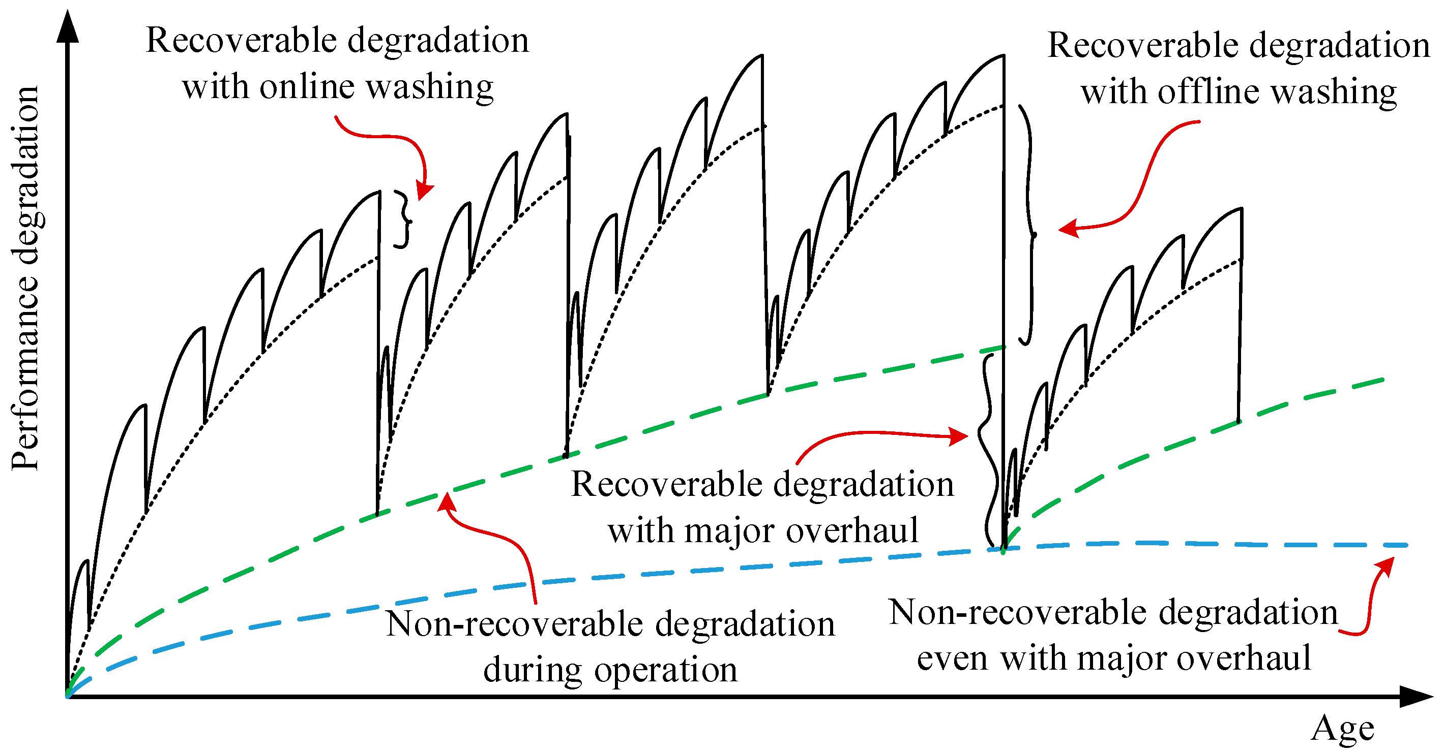
The performance of a gas turbine degrades during operation due to internal and external abnormal conditions. Fouling, erosion, corrosion, and increased tip clearance are among the most common gas path problems. As illustrated in Figure 1, gas turbine degradation can be recoverable and non-recoverable [35]. The former is mostly recoverable through effective online and offline compressor washing with major inspection during engine overhaul. Degradation due to fouling is the most prominent example here. The latter refers to the residual deterioration remaining after a major overhaul, which can be considered as a permanent performance loss. Mechanical wear caused by erosion and corrosion may lead to airfoil distortion and untwisting, thereby resulting in non-recoverable performance loss. Both recoverable and non-recoverable degradation should be monitored continuously for optimal maintenance scheduling.
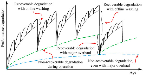
Figure 1.
Recoverable and non-recoverable engine degradation; adapted from [35].
Degradation can also be categorized as short-term and long-term based on the formation and growth rate [36]. Short-term degradation results in fast performance changes and is usually caused by fault events. As shown in Figure 2, they can manifest themselves as “abrupt” or “rapid” degradation modes. Abrupt faults are fault events that appear instantaneously and remain fixed in magnitude with time, for instance sensor bias, actuator fault, foreign object damage/domestic object damage (DOD/FOD), and system failure. Rapid faults refer to fault events that initiate and grow in magnitude with time. Gradual degradation refers to gradual performance losses that develop slowly and simultaneously in all engine components over time due to mechanical wear, mainly triggered by erosion and corrosion [37]. The performance loss due to gradual degradation increases through time and may reach a non-restorable stage. For a detailed description about different degradation mechanisms, their effects, and necessary actions to restore performance losses, the interested reader is referred to [1,38].
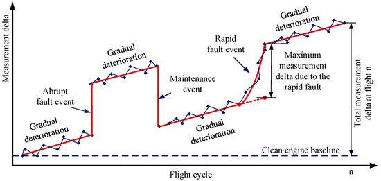
Figure 2.
Long-term vs. short-term deterioration.
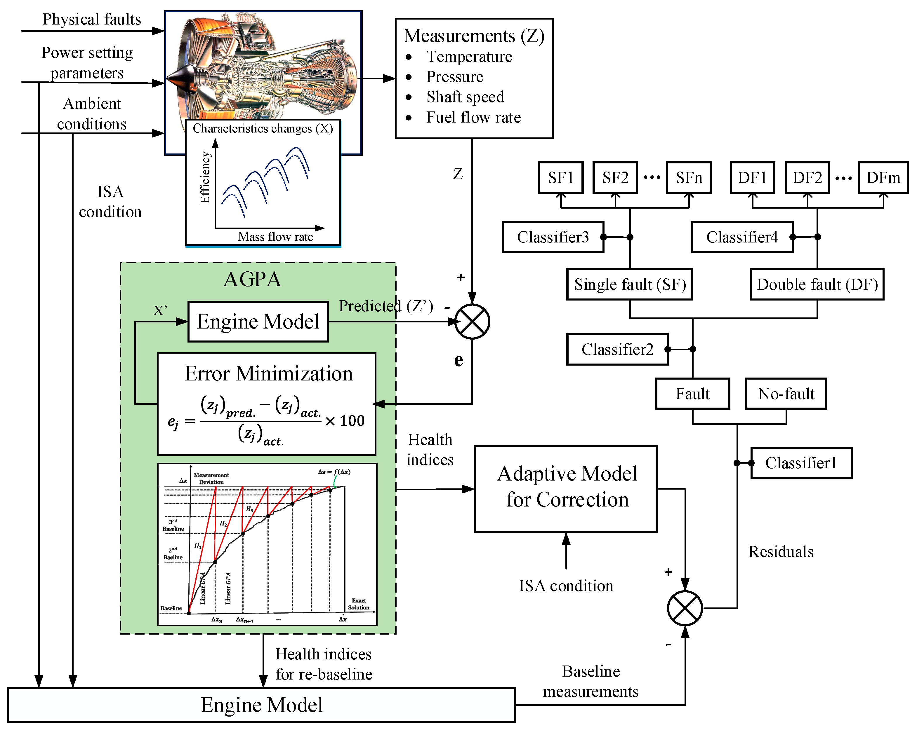
A diagnostic system for life-cycle assessment should be able to distinguish short-term and long-term degradation modes followed by detecting and isolating faults successfully [39]. If the diagnostic algorithm is not adaptive to trend shifts due to engine degradation, its effectiveness will eventually decrease with the engine age. This is more problematic for most of the data-driven techniques, since baseline shifts may cause differences between training and test data patterns, which potentially could affect the diagnostic accuracy. One of the possible solutions to overcome this problem is incorporating AGPA in the diagnostic system. In AGPA, the model adapts performance trend changes with time and updates the baseline when it is convenient. Measurement deviations with respect to the deteriorated engine profile can then be used to assess gas turbine faults based on machine-learning techniques. However, using AGPA alone has some accuracy deficiencies due to measurement uncertainty and model smearing effects [40].
3. Methodology
3.1. Proposed Method
A schematic of the proposed gas path FDI system is illustrated in Figure 3. The system was designed to accommodate both long-term and short-term degradation problems. This procedure involves three main steps: trend monitoring to compute performance parameter deltas due to the two degradation effects, generate measurement deltas, and detect and isolate component faults in the engine gas path based on sets of CNN modules. Each of the steps is described in more detail below.

Figure 3.
Schematic of the proposed FDI system.
3.1.1. Trend Monitoring and Measurement Pattern Generation for the Data-Driven Method
An adaptive scheme described in [40] was applied to monitor the trend of the engine performance in terms of performance parameter deltas (Δη, ΔΓ) and discriminate between gradual degradation and rapid faults. The algorithm adapts to the engine degradation with the purpose of calculating Δη, ΔΓ from the gas path measurement changes through an iterative process. If changes occur due to ambient and flight condition variations, the adaptive scheme can correct the data with respect to these variations. However, the data correction part was not included in the current work since it has been discussed thoroughly by the authors previously [40,41].
For a gradual degradation, all the health parameters are expected to deviate together from the first flight up until the engine overhaul. The increment of the loss between each subsequent flight should not noticeably exceed the expected value. For instance, the isentropic efficiency and flow capacity parameters of a twin spool low-bypass turbofan engine LPC showed a −2.61% and −4% deviation after 6000 flights, respectively [37]. That means ~−0.00044% and ~−0.00067% in the firsts flight and ~−0.0044% and ~−0.0067% in the tenth flight if a linear progress is considered. When a rapid fault occurs in one or more of the gas path components, the corresponding performance parameters show considerable shifts from the gradual trend. To estimate the net measurement changes induced by the underlying fault(s), first, a new baseline should be established at some previous flight α and the performance parameter deltas computed backwards from the current flight k to flight α + 1, as illustrated in Figure 4 and Figure 5. Second, we used the estimated performance parameter deltas to predict corrected measurements through the engine performance model in adaptive mode at the reference conditions (i.e., TRef = 288.15 K and PRef = 1.01325 bar). Then, we set the corrected measurements at flight α as new baseline measurements. For the subsequent flights (from flight α + 1 to flight k), we took the actual measurement at each flight and ran the gas path analysis to estimate the associated performance parameter deltas with respect to the new baseline. We repeated the second step and predicted the associated corrected measurements. Finally, we computed the measurement deltas based on Equation (1).
where is the corrected and normalized value of the jth sensor at the ith flight, is the corrected value of the jth sensor at the ith flight to be normalized, and is the reference value of the jth sensor at the new baseline.
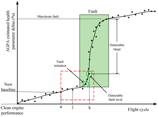
Figure 4.
Schematics of performance tracking and re-baselining.
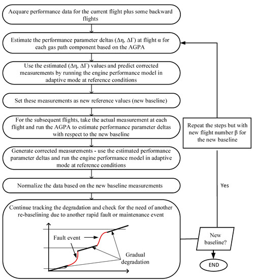
Figure 5.
Re-baselining and measurement pattern generation steps.
If maintenance actions take place after a rapid or abrupt fault event, the level of performance recovered needs to be assessed. The level of the recovery depends on the type and effectiveness of the maintenance action taking place. It could be evaluated by comparing with the performance of the engine when it was brand new or by comparing it with the re-baselined performance just before the fault occurs. If there is a considerable unrecovered performance left after the maintenance, re-baselining will take place after the maintenance event to re-use the model ahead.
One important point to be noticed here is that event faults should not be declared based on a single point trend shift since this might happen due to a statistical outlier. There is a trade-off between detection delay to avoid potential false alarms due to outliers and quick fault detection to avoid potential catastrophic damages in the subsequent flights [42]. An effective measurement noise reduction could minimize the risk. Otherwise, the detection algorithm must be robust enough to handle noise. In this regard, data-driven methods have proven advantages over model-based methods [40,43].
3.1.2. Convolutional Neural Networks
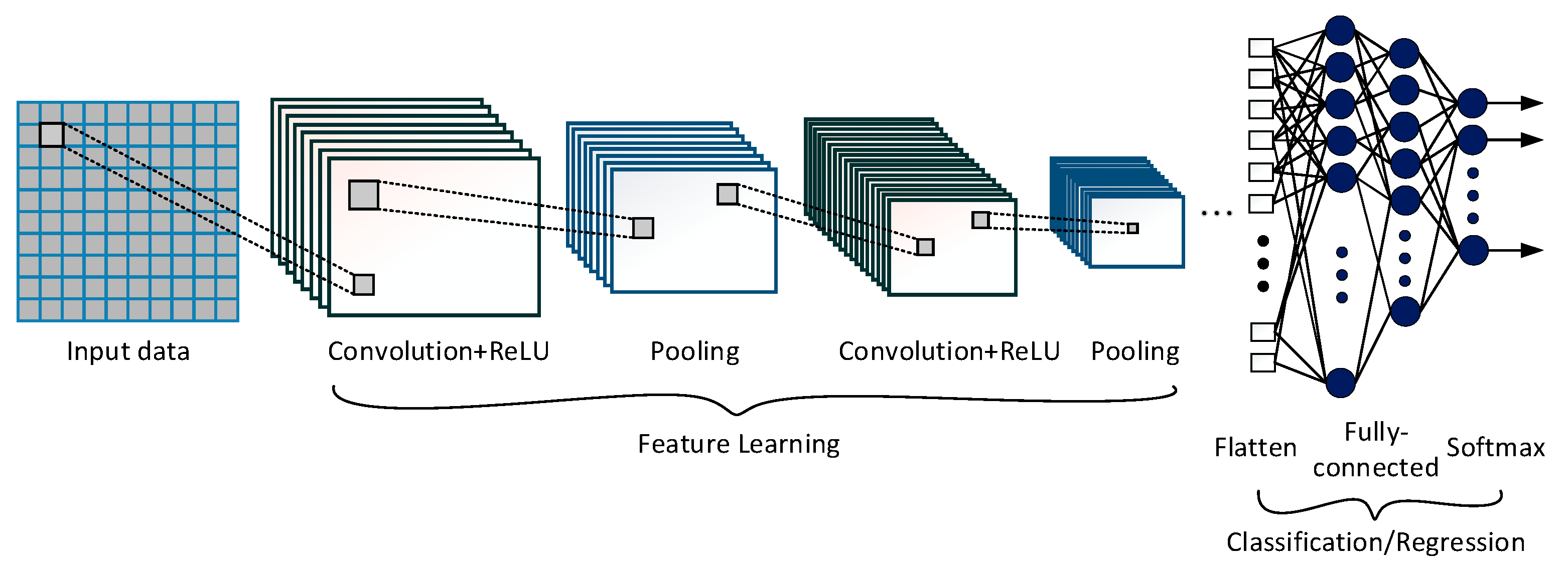
Convolutional neural networks [44] are an important family of deep-learning neural networks that have so far been most commonly used for image classification and computer vision. Recently, considerable attempts have also been made to use CNN for machinery diagnostics and prognostics. There are several emerging variants of CNN architectures with different degrees of complexity. LeNet, AlexNet, VGGNet, and GoogLeNet are among them. A typical CNN architecture may consist of an input layer, convolutional layer, activation layer, pooling layer, fully-connected layer, and output layer, as illustrated in Figure 6. It takes input information via the input layer, which passes through sets of layers with a series of operations and then gives qualitative or quantitative outputs based on its purpose. Feature learning and classification are the two sub-sections of a CNN structure, where the former is used to extract the most useful features from the input data, while the latter maps the extracted features into the final output. A more detailed discussion on its structure and functionality is available in the open literature [44]; however, a brief description of the main layers is provided herein.

Figure 6.
The general structure of the CNN.
Convolutional Layer
Convolutional layers are the basis of a CNN model. They convolve sets of filters (kernels) over the input information and generate single or multiple representative feature maps. Convolution takes place by sliding the filter across the input data. For every slide, the output is the dot product of the filter and the part of the input data to which the convolution operation is applied. This can mathematically be expressed as:
where is the output of the convolution for the filter k in layer l, is the input of that layer, f(᛫) represents the activation function, and w and b refer to the corresponding weight (filter) and bias values, respectively.
Pooling Layer
The pooling layer is also called the downsampling layer or subsampling layer. It is the next layer of the convolutional layer, where the convolved features are dimensionally reduced by pooling. Maximum pooling and average pooling are the two most widely used pooling methods [24]. The former extracts the most useful features within a subset of an input feature map, whereas the latter considers the average value. Max pooling was applied in this research since it extracts the most relevant features within the convolved feature map.
Fully-Connected Layer
The structure and function of the fully connected layer is the same as in a conventional multilayer perceptron. It is in essence a backpropagation-based feed-forward neural network. The typical structure is composed of input and output layers with one or more hidden layers in between. The role of this layer in the CNN operation is mainly to produce a meaningful output from the extracted features. Since the fully-connected layer does not allow multi-dimensional data input, the feature output from the feature-learning section needs to be flattened [30].
Output Layer
The output layer performs the final operation in the CNN model. Softmax (Equation (3)) is one of the most widely used functions in classification [24]. It computes probabilistic values to make the class decision about where the input data belong. The probability values estimated for each class considered in the classification problem sum to one.
where S is the softmax function, is the input feature vector, is the standard exponential function for the input feature vector, c is the number of classes in the classification problem, and is the standard exponential function for the output.
3.1.3. Engine FDI System Using Modular CNN Classifiers
Although different authors including Volponi [45] have argued that there is very little chance for two or more rapid faults to occur simultaneously, public benchmark studies from NASA [33] recommend considering multiple faults for more trustworthy diagnostic solutions. The probability of having simultaneous faults depends on the flight environment (e.g., rainy, sandy, salty, dusty, smoky, etc.) and the level of severity. In the current work, single- and double-component faults were considered in a three-shaft turboshaft engine. A modular CNN-based FDI algorithm was developed for this purpose in order to step-by-step solve the engine problem to the component level. Using hierarchical networks is also a common practice in image classification and has shown considerable advantages, because it allows capturing the feature relationships between groups and subgroups. It also helps to share the classification burden between a bank of classifiers arranged hierarchically. Four different classification modules dedicated to handling specific tasks were used. The first module (Classifier1) was trained to detect the presence of a fault. Classifier2 is activated following a fault detection to distinguish between the single- and double-fault category. The last two classifiers (Classifier3 and Classifier4) were trained to distinguish the affected component(s). Classifier1 and Classifier2 are binary, whereas Classifier3 and Classifier4 can be either binary or multi-class classifiers depending on the number of faults they are assigned to handle.
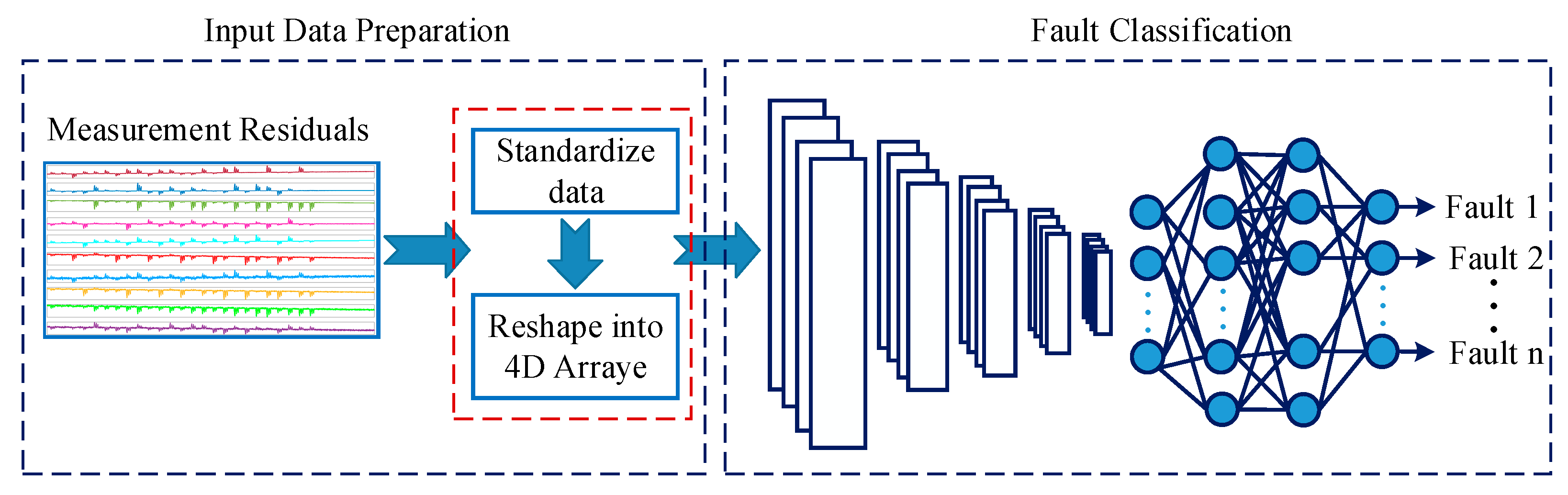
The complete activity of the fault analysis has two steps, as illustrated in Figure 7: input data transformation and fault classification. The first step involves standardizing the input data to enable the unbiased contribution of each measurement and enhance the classification performance. Reshaping follows to convert the input data from a matrix format to a 4D array, which can easily be used by the CNN model in MATLAB. In the next step, the CNN algorithm was trained to extract features from the input data and map those features to the fault classes considered. These steps are discussed further below.
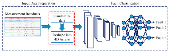
Figure 7.
The general procedure of the fault classification applied: input data standardization/scaling, data reshaping, and fault classification using CNN.
3.1.4. Input Data Preparation
In the field of machine diagnostics, using the CNN for fault classification was inspired by its powerful feature learning and image recognition ability via imitating the image-processing concept. This often requires a 2D data structure (or image), which is different from the typically available 1D time series signals. Various signal transformation techniques have been applied to convert signal data to images, including image transformation, matrix transformation, time/frequency domain transformation, wavelet transformation, and short-time Fourier transformation [24]. In the current experiment, the generated measurement patterns were in a matrix format with a shape of (N × M), where M is the number of measurement parameters with N the number of samples. Min-max normalization (Equation (4)) was implemented to scale the data to the range of −1 and 1. The data were then transformed into a 4D array of shape ((width, height, channel, sample size) as (rows, columns, channels, sample size)). Accordingly, the matrix data were converted into the shape of (1, M, 1, N). While fitting the data to the CNN model, each of them was considered an image with a dimension of width = 1, height = M, and channels = 1.
where is the scaled value of signal , is the original ith signal of the jth sensor, is the minimum value of the jth sensor, is the maximum value of the jth sensor, , and .
3.1.5. CNN Architecture and Training
The architecture of the CNN model used in this paper was determined through a training process. As described in Table 1, it consisted of two consecutive convolutional layers followed by a single pooling layer with a ReLU [46] activation function and a dropout layer in between. ReLU is a piecewise linear function that outputs zero when the input value is negative and outputs the input as it is when the input is ≥0. This activation function is popular in CNNs since it overcomes the vanishing gradient problem and often achieves better performance [24]. The first convolutional layer contains 112 filters of size 1 × 10 with a stride 1 × 1, whereas the second convolutional layer contains 212 filters of size 1 × 2 and stride 1 × 1. In these two convolutional layers, the input information is convolved to capture representative signatures on the associated output feature maps. A maximum pooling layer with filters of 1 × 2 and stride 1 × 1 was used for the downsampling operation. A second dropout layer was added right after the pooling layer, followed by a single fully-connected layer. The final layer of the structure is the output layer, which is used to determine the class type based on probability distributions estimated by the softmax function. The Adam optimization algorithm was the learning algorithm selected, which is an extension of the classical stochastic gradient descent learning scheme [47]. It has the benefits of high computational efficiency along with little memory requirement. Similar hyperparameters are applied for all the CNN models in the proposed hierarchy.

Table 1.
Details of the CNN architecture and learning hyperparameters.
In deep learning, training good models is challenged by the overfitting phenomenon. This phenomenon must be controlled to achieve a more generalized solution. In CNNs, overfitting can be handled either by involving the so-called “dropout” operation or based on cross-validation. The former technique was introduced by Srivastava et al. [48]. It is accomplished through randomly and temporarily dropping some hidden neurons within the CNN structure. The latter applies a training stopping criterion using a dataset other than the one used for training. Here, the network training should stop when the validation error begins to increase while the training error keeps on decreasing. Zhao and Li [30] applied the cross-validation technique in their suggested CNN-based gas turbine diagnostic method. Using deep ensemble methods could also be considered as an alternative approach to overcome overfitting, as well as quantify the uncertainty in the predictions made [49]. In the current paper, the authors applied the dropout concept with 30% dropouts to each dropout layer involved in the structure.
3.2. Method for Comparison
3.2.1. Single CNN Classifier
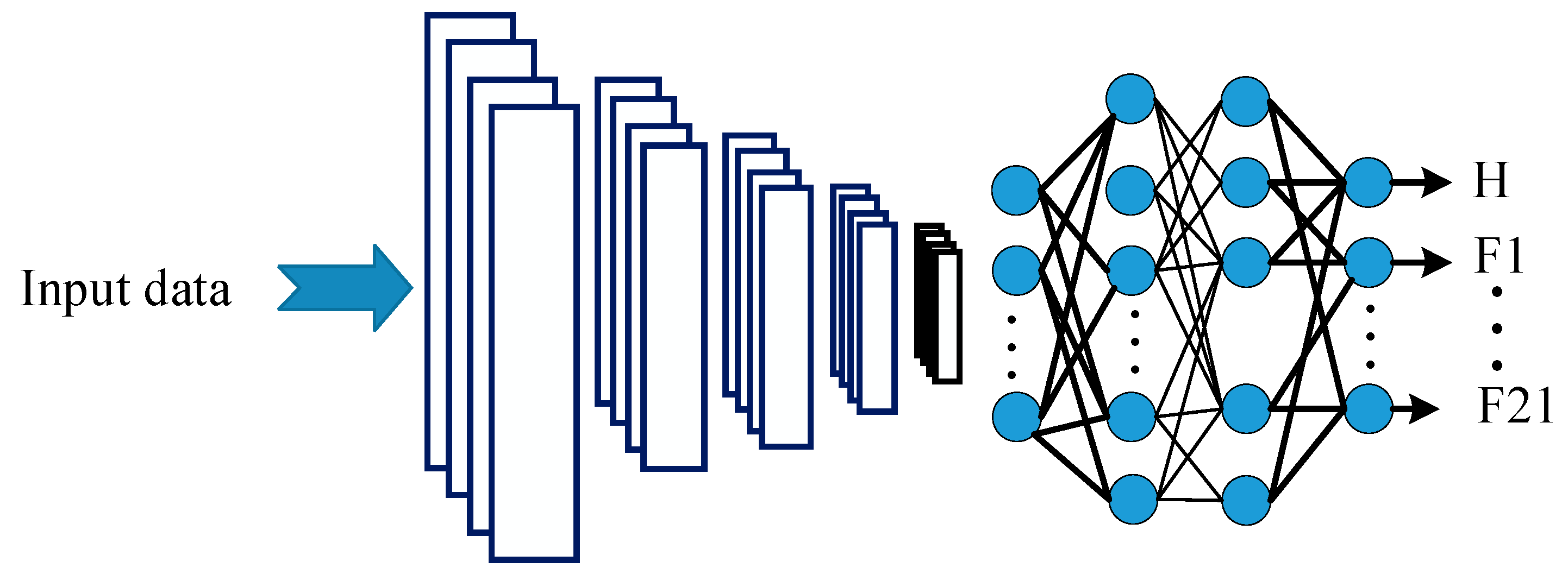
An alternative CNN classifier was applied for comparison purposes. As illustrated in Figure 8, a single CNN structure was trained to classify all the 22 engine conditions considered in this work, instead of multiple hierarchical CNN classifiers. Similar hyperparameters and learning datasets as applied to demonstrate the proposed method were utilized.

Figure 8.
Schematics of the classical single network-based CNN classifier.
3.2.2. Long Short-Term Memory
The performance of the proposed algorithm was further compared with an LSTM-based classification algorithm. LSTM is a special kind of recurrent neural network (RNN) in the deep-learning domain that can learn long-term dependencies from time series data and capture the relations between input variables through backpropagation. It is more popular in time series and sequence classification and prediction problems. Recently, considerable reports have been presented on its application for system and rotating machinery health management [24,50] including gas turbine prognostics [51,52,53]. There were also a few attempts to employ LSTM for gas turbine diagnostics as well [54].
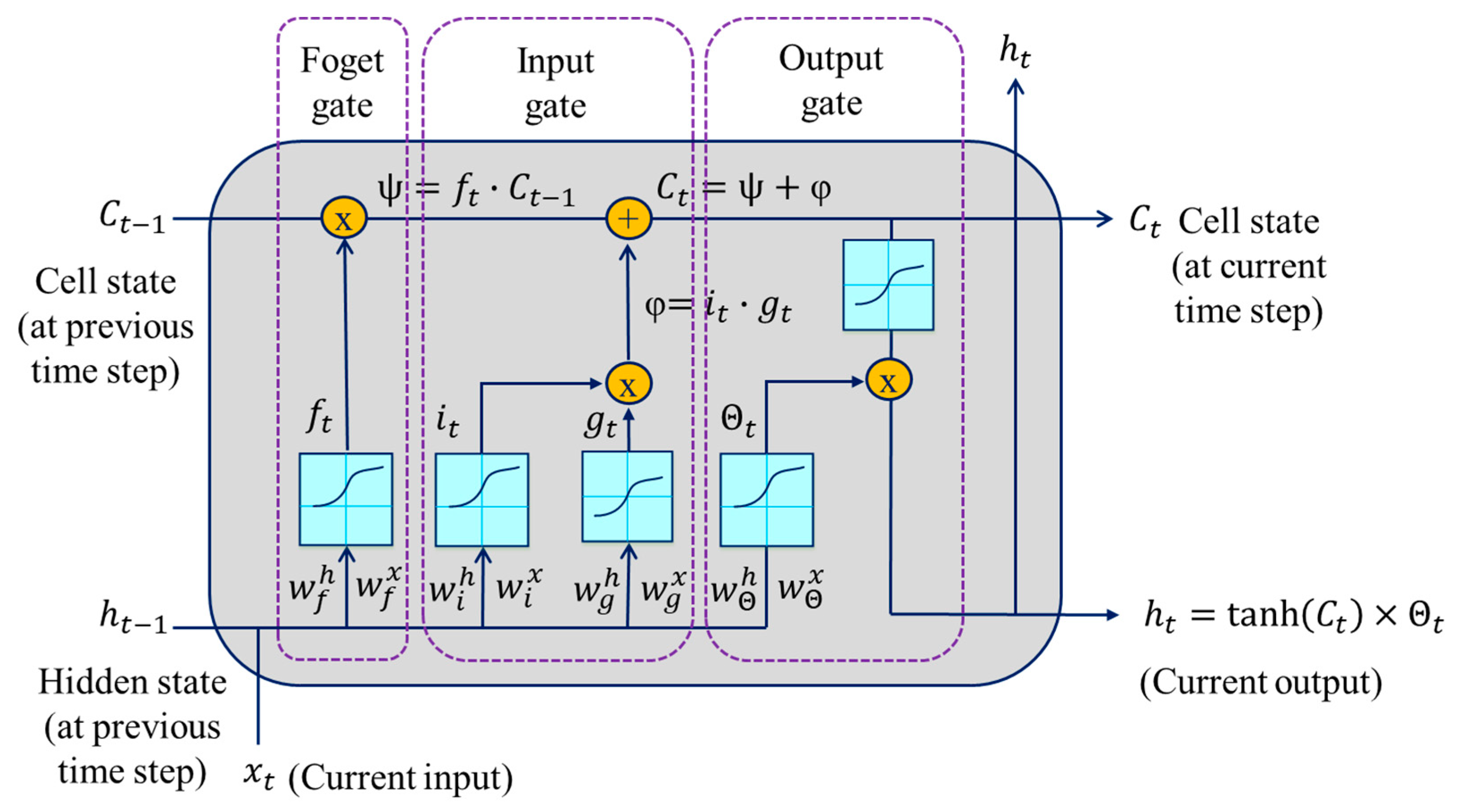
The typical LSTM architecture for classification consists of an input layer, an LSTM layer, followed by a standard feedforward output layer. The LSTM layer encodes the input information in the time series or sequence via its memory unit or cell. Figure 9 shows an LSTM unit with its three information regulators called gates (forget gate, input gate, and output gate). The cell remembers values over arbitrary time intervals, while the input and output gates regulate the information flow into and out of the cell, respectively.
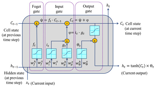
Figure 9.
Schematics of a single LSTM cell with its three gates.
Based on the connections shown in Figure 9, the mathematical expressions used to compute the outputs from the gates and the LSTM cell can be formulated as:
where σ denotes the sigmoid activation function, ht−1 and Ct−1 refer to the previous hidden state and cell state, respectively, and xt is the current input. ft, it, Θt, Ct, and ht are the forget gate, input gate, output gate, cell state, and hidden state at time step t, respectively. and denote the forget gate weights associated with the hidden state and the input, respectively. and refer the input gate weights associated with the hidden state and the input, respectively. and are the output gate weights associated with the hidden state and the input, respectively. is a cell candidate in the input gate used to add information to the cell state. and represent the weights associated with the hidden state and the input, respectively. , , , and denote the forget gate, input gate, cell candidate, and output gate bias, respectively.
LSTM can be modeled as a unidirectional LSTM (ULSTM) or bidirectional LSTM (BiLSTM). In the former case, information flows in one direction, while the latter is an extension of the former in which information flows both forward and backward. Some studies indicated that the BiLSTM model provides better predictions than ULSTM, but with a greater training time [55]. As presented in Table 2, four different LSTM models were considered for this comparison. Each model is composed of seven layers: an input layer, two LSTM layers with a dropout layer right after each LSTM layer to control overfitting, a fully connected layer, and an output layer. Model 1 and Model 2 exploit ULSTM and BiLSTM, respectively, while Model 3 and Model 4 use a combination of the two, but in a different order. Then, as shown in Table 3, each model was employed to perform the step-by-step classification tasks described in Section 3.1.
Table 2.
LSTM-based comparison models.
Table 3.
Compared LSTM models at different stages of the fault classification.
3.3. Performance Evaluation Metrics
The performance of the detection module, Classifier1, was evaluated based on five indicators: true positive rate (TPR), true negative rate (TNR), false positive rate (FPR (or false alarm rate (FAR)), false negative rate (FNR) (or missed detection rate (MDR)), and overall detection accuracy (ODA). Similarly, different classification performance indicators were implemented for Classifier2, Classifier3, and Classifier4 based on classification confusion metrics (Table 4). These indicators were adapted from [39,56] and briefly described below:
Table 4.
Multiclass classification confusion matrix and evaluation.
Overall classification accuracy (OCA): Diagonal cells of the decision matrix contain the number of correctly classified fault cases associated with each fault considered in the classification. The ratio of the sum of these cases and the total number of cases used in the classification gives the OCA of the algorithm. However, since OCA indicators can be misleading, the classification accuracy for each fault class should also be assessed for a complete and meaningful picture. That means there is a possibility to have a high OCA, while individual fault classification results show considerable errors;
Correct classification rate (CCR) (also called recall): This indicates the number of correctly classified fault cases with respect to each fault class. The CCR can be described as the number of correctly classified fault cases divided by the total number of cases in that particular fault (refer to Column 8 of Table 4 for the mathematical expression);
Incorrect classification rate (ICR): Incorrect classification occurs when the classifier wrongly predicts some fault data points as another class that do not belong to it. It is calculated by dividing the sum of wrongly classified cases to the total number of cases used for that fault (ICR = 1 − CCR; Column 9 of Table 4);
Precision (Pr): Precision is another useful classification accuracy index for a fault class. It is the ratio of correctly classified cases of a fault to the total number of cases predicted as belonging to that fault type (refer to Row 8 of Table 4 for the mathematical expression). Precision error (PrE) = 1 − Pr;
Kappa coefficient (KC): This measures the degree of agreement between recall and precision. The value of the KC is always less than or equal to one. If KC ≤ 0, then there is no agreement between the predicted and true value. If KC = 1, then the classification is perfect. Hence, the higher the KC, the more accurate the classification is. Let Ftp represent the cell value of the fault in the confusion matrix (where t refers to the true class and p the predicted class), then the KC can be expressed as:
3.4. Synthetic Data Generation
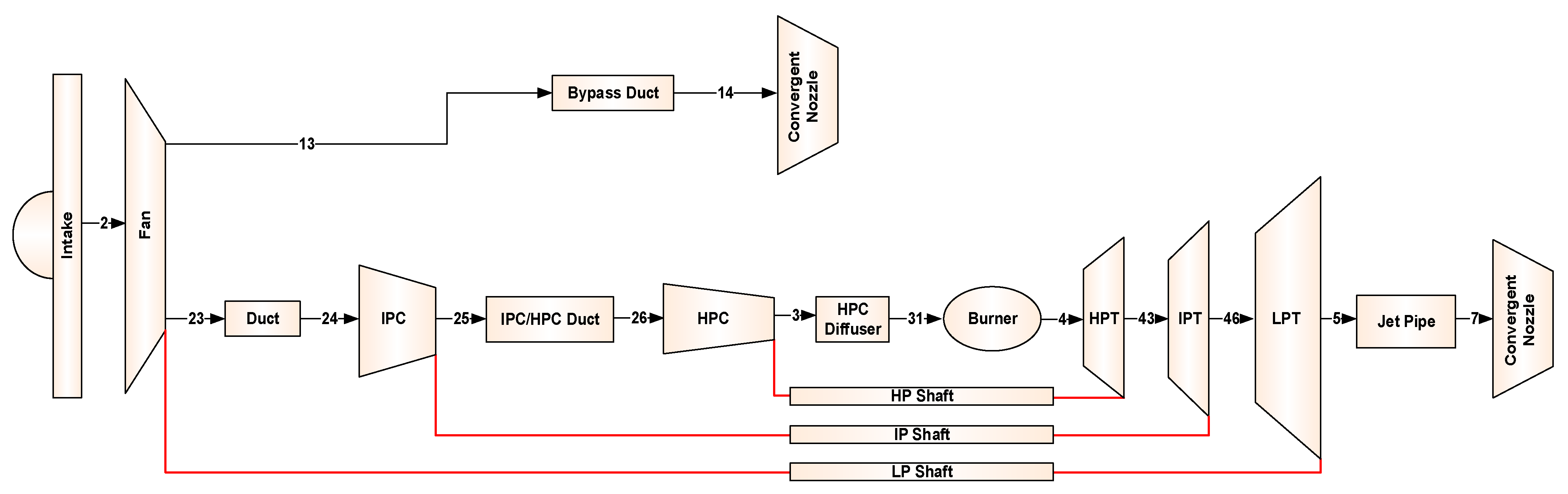
The data required to demonstrate and validate the proposed method were generated from a performance model of a three-shaft turbofan engine. This involved both gradual and rapid degradation scenarios at a steady-state condition. An in-house engine simulation software, called EVA [57,58], was used for this purpose. The tool can perform simulations for any kind of gas turbine engine in any configuration under both steady-state and transient operating conditions. Figure 10 illustrates the schematics of the engine under consideration with the locations of the measurement stations. The description of each measurement used for the engine diagnostics with the associated level of noise considered is provided in Table 5. Gaussian noise was added for each measurement with a standard deviation (σ) in percent of the measured values. The model is thermodynamically similar to a 70,000 lbf-class engine with technology levels consistent with entry into service in 1995. Some specifications at top of climb are provided in Table 6. In the present work, the FAN, intermediate-pressure compressor (IPC), high-pressure compressor (HPC), high-pressure turbine (HPT), intermediate-pressure turbine (IPT), and low-pressure turbine (LPT) were selected as the target gas path components due to their exposure to degradation.
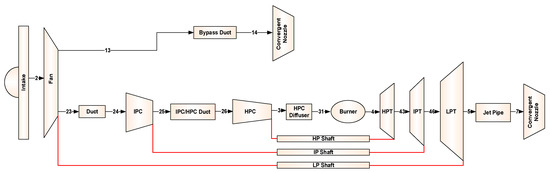
Figure 10.
Schematics of the three-shaft turbofan engine with measurement locations.
Table 5.
Sensors’ list with the considered noise level.
Table 6.
Nominal conditions at top of climb.
3.4.1. Gradual Degradation Simulation
Gradual degradation was simulated by simultaneously adjusting the flow capacity and efficiency deltas (∆η, ∆Γ) of the six gas path components (FAN, IPC, HPC, HPT, IPT, and LPT) based on the values provided in Table 7 [37]. Since the type of gas turbine studied in [37] was a two-shaft turbofan engine (which means it did not have an LPT), a similar level of degradation as that of the IPT was considered for the LPT of the current engine. The modification factors were implanted into the performance model of the engine, starting from zero to the maximum values and assuming linear degradation trends. Initial wear (i.e., at flight cycle = 0) due to manufacturing inefficiencies was not considered. Since the gradual degradation was not considered a fault for a short period, the measurement deltas associated with this degradation were used as a baseline to estimate the measurement residuals due to rapid faults.
Table 7.
Engine performance losses in percent due to gradual degradation in terms of efficiency and flow capacity deltas; adapted from [37].
3.4.2. Rapid Degradation/Fault Simulation
A total of 21 gas path faults (6 single-component faults (SCFs) and 15 double-component faults (DCFs)) were considered, as presented in Table 8. For each fault type, modular faults were simulated by simultaneously adjusting the ∆η and ∆Γ values based on Equation (12). Pattern generation was then performed, as explained in Section 3.1, to find patterns of measurement deviations (residuals) due to measurement noise and actual faults. In this case, measurements from the gradual degradation were taken as references. Significant measurement noise was included in the data based on Table 5, to evaluate the tolerance of the diagnostic system against measurement uncertainty effects.
Table 8.
Description of faults considered.
The listed faults in Table 8 were randomly implanted into the model in the occurrence of gradual degradation. Each fault was assumed to cover 200 flights from initiation to reaching its maximum severity. When the next fault scenario started, we set the previous fault scenario to zero, and so on, until the last fault scenario occurred. Accordingly, 176,940 samples were extracted from this degradation profile for the CNN demonstration under different noise levels. For the 12 sensors (T23, P23, T25, P25, T3, P3, N4, N44, N46, P43, P46, and P5) considered in this work, the data became a matrix of 12-by-176,940. This data were then scaled and converted into a 4D array of shape (1, 12, 1, 176,940) in preparation for the CNN model. We divided it into different groups while conducting the training.
4. Results and Discussion
We performed a modular-CNN-based engine fault detection and isolation for a triple-spool turbofan engine application. In this framework, four CNN modules were trained individually and connected in such a way that they could first detect a fault and then isolate to the component level. A series of experiments was carried out aiming to select the optimal CNN structure associated with each classifier. The impacts of the important hyperparameters in the CNN training including the number of filters and size, number of layers and order of arrangements, type of optimization algorithm, and number of epochs were analyzed. For instance, different numbers of filters in the range of 1–256 were investigated.
Based on the training results, a similar CNN architecture was selected for all modules involved in the framework. The only difference was the training data size used and the number of outputs associated with the classification problem to which they were assigned. For each classification module in the hierarchy, the selected architecture with the best performance consisted of double consecutive convolutional layers followed by a single pooling layer, including ReLU and dropout layers in between. Considering a second convolutional layer, with an increased number of filters and decreased filter size compared to the first convolutional layer, we demonstrated better classification performance. For all modules, 20 epochs (27,640 iterations with 1382 iterations per epoch) were required to reach the maximum accuracy. Adam was the optimization algorithm utilized primarily due to its simplicity and little memory requirement.
4.1. Fault Detection
The best classification results for CNN1 are presented in Figure 11. The results on the main diagonal of the detection decision matrix show the number of correctly detected patterns with respect to the health and fault class, whereas the values to the right and left side of the diagonal represent wrong detections. As presented in Table 9, the detection accuracy of the algorithm was then assessed in terms of the standard fault detection accuracy indicators. Ideally, a fault detection system is required to have negligible false alarm and missed detection rates, but this is practically difficult to achieve due to several factors including measurement noise, feature extraction limitations, and insufficient sampling [59]. When the detection system becomes more sensitive to faults aiming to provide early warnings and avoid unexpected failures, the frequency of false alarms rises. A high false alarm rate is one of the common problems of the traditional threshold-based gas turbine health management technologies [59]. This may be among the reasons why high feature extraction techniques have been receiving more attention in resent studies. As shown in this figure, generally, a 95.9% overall detection accuracy was achieved with a 0.4% FAR and a 13.2% MDR. The TPR was low because low-level faults up to 0.025% (i.e., ∆η = 0.01% and ∆Γ = 0.02% according to Equation (12)) were considered. About 20% of the fault data were generated from fault magnitudes ≤1%. This indicates that increasing the lower detectable fault, say for example to 0.25% will enhance the detection accuracy considerably by increasing the TPR and decreasing the FAR. Hence, considering the measurement noise effects, the obtained FAR and MDR values are encouraging.
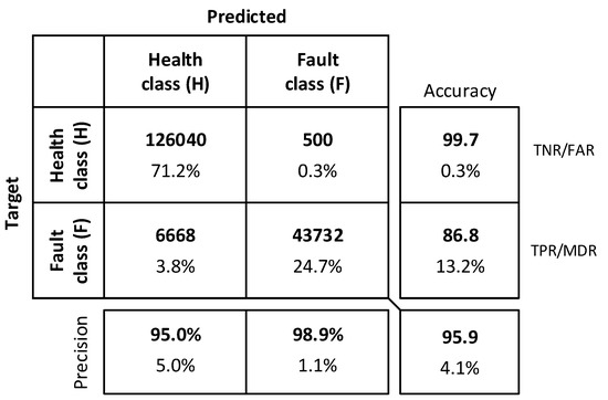
Figure 11.
CNN1 detection accuracy with the Adam optimization algorithm.
Table 9.
Comparison of Adam, sgdm, and RMSprop optimization algorithms.
The effect of the optimization algorithm on the classification performance was also investigated. A comparison was made against two other popular algorithms, namely stochastic gradient descent with momentum (sgdm) and root-mean-squared propagation (RMSProp) [60], under similar circumstances. As shown in Table 9, all three optimizers had similar performances with a maximum overall accuracy difference in the order of 1%. Nevertheless, as Adam is known for its low memory and computational requirements and has some additional advantages in deep-learning applications [60], it was selected for training all CNN models in the proposed framework.
Effect of the Data Distribution
It is known that the accuracy of deep-learning methods often relies on the amount of data available for training, and the degree of dependency differs from case to case [61]. Increasing the training sample until it becomes enough to represent the distribution of the data required to define the nature of the problem under consideration usually improves the prediction accuracy. However, memory and computational burden should be taken into consideration. Using a high-performance computer (HPC) or GPU can overcome this problem. Another important factor to be noted is that the distribution of the datasets representing the two classes should not be skewed. This is because most ML algorithms often experience poor classification performance due to the high chance of biasedness to the majority class. In contrast, imbalanced data availability is a common problem in fault detection, since in real-life operations, most of the samples available are for the healthy state of the asset [31]. In this experiment, six different randomly selected datasets of size 72,000 (≈30%H and 70%F), 92,988 (≈46%H and 54%F), 113,976 (≈56%H and 44%F), 134,964 (≈63%H and 37%F), 155,952 (≈68%H and 32%F), and 176,940 (≈72%H and 28%F) were considered for CNN1. In all these datasets, the same 50,400 fault cases were used. There were 30% random dropouts applied right before the pooling layer and fully-connected layer to control the overfitting problem.
Table 10 summarizes the detection results obtained based on the six data groups. The results revealed that the overall detection accuracy increased with increasing the sample size. For example, increasing the size from Set-1 to Set-2 enhanced the ODA by 1.8% with a 3.2% lower FAR and a 1.5 higher MDR. When Set-6 was applied instead, the ODA rose by 5.2%, while the FAR dropped by 6.1% and the MDR rose by 2.6%. The observed differences in the calculated performance indicators were because of the difference in the healthy-to-faulty data proportion among the six data groups.
Table 10.
Effect of data size on the detection accuracy of CNN1.
4.2. Fault Isolation
The next step in the diagnostic process is root cause determination (or fault classification). Upon fault detection through CNN1, the underlying faults were isolated applying CNN2 followed by CNN3 and CNN4. The classification results obtained from CNN2, CNN3, and CNN4 are presented in Table 11, Table 12 and Table 13, respectively. The classification accuracy indicators described in Section 3.3 were used. For CNN2 and CNN3, an OCA performance better than 99% and for CNN4 an OCA performance better than 98% were achieved. Similarly, KC values higher than 0.98 were obtained for all three models. The ~1% accuracy difference between the CNN3 and CNN4 modules was expected due to: (1) the difference in the number of faults that they were responsible for and (2) the difficulty of simultaneous fault classification. On the other hand, the similar accuracy observed for different fault states within a classifier could be due to the equal data size contribution of each class in the training dataset and their relationship (the slight accuracy differences were expected due to the nature of the training itself). Model complexity and computational requirements were found to reduce from top to bottom. This can be attributed to the difference in the number of classes involved corresponding to each module, as well as the learning data size used. Overall, the obtained results demonstrated the excellent potential of CNNs for engine gas path components’ FDI.
Table 11.
CNN2 classification accuracy assessment results.
Table 12.
CNN3 classification accuracy assessment results.
Table 13.
CNN4 classification accuracy assessment results.
4.3. The Proposed Method vs. a Single Network Classifier
A single CNN model was trained to classify the 22 classes at once, and the results were compared with those of the proposed method. As reported in Table 14, the model achieved a 96% overall accuracy with a 0.9167 KC. Although both the OCA and KC indicators appeared to be high, the accuracy recorded for some of the faults, for instance F3, F6, F12, and F18, showed considerable errors. Using such a single network to assess the health of the entire gas path system has additional disadvantages: (1) the complexity of the model increases with the increasing number of faults; (2) a fault detection should first take place before any further investigation is performed; (3) high computational burden. This may be the reason why recent studies have been paying more attention to multiple model approaches [62].
Table 14.
Engine fault classification accuracy based on the single CNN structure.
4.4. CNN vs. LSTM
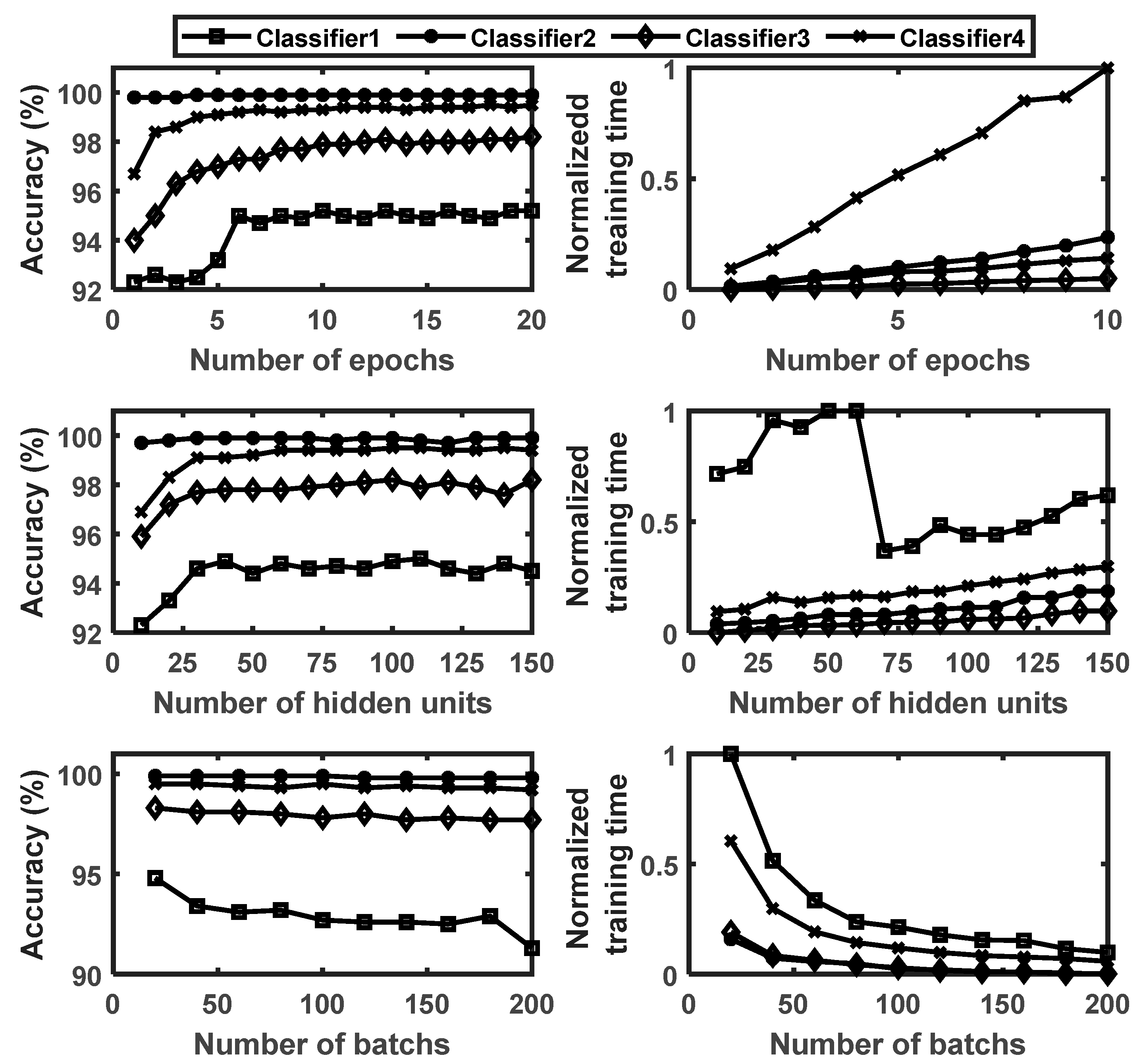
As the CNN, the best architecture for each classification module in the hierarchy was determined through a training experiment. The hyperparameters considered in the investigation include the number of layers, number of hidden units in each LSTM layer, number of dropout layers and their corresponding percentage dropout values to avoid overfitting, the batch size, and number of epochs required to complete the training. The efficient Adam optimization algorithm was used for all models. Figure 12 shows the influence of the number of epochs, hidden units, and batches on the classification accuracy and training time of the four ULSTM modules. For an arbitrary batch size and number of hidden units, the classification accuracy increased with increasing epochs up to 10. Thenceforth, the accuracy did not change significantly. Similarly, for a given random number of epochs and batch size, the accuracy increased with the increasing number of hidden units up to 40 and showed negligible changes from there on. On the other hand, it was observed that both too small and too high batch size values reduced the accuracy. In all the cases, the highest training time recorded was for Classifier1 due to the data size used for training. However, training time could not be an issue if high-performance computers/hardware, such as GPU, or parallel computing are used.
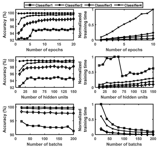
Figure 12.
Number of epochs, number of hidden units, and batch size vs. classification accuracy and training time for the ULSTM classifiers.
Based on the training performances, the number of epochs, hidden units, and batches were fixed as 10, 70, and 100, respectively, for all classifiers. The comparison results presented hereafter were based on these hyperparameters. Table 15 and Table 16 present the fault detection and fault classification comparison results obtained, respectively. The detection results revealed that both the CNN and LSTM methods considered in this comparison showed similar accuracy. ULSTM-BiLSTM1 should some advantages in terms of the FAR (0.2% lower than CNN1, 0.3% lower than ULSTM1 and BiLSTM-ULSTM1, and 0.4% lower than BiLSTM1), but on the other hand, it showed the lowest TPR (87%) and ODA (96%). CNN1 had the highest ODA (96.5%) and true positive rate (89.2%) and the second lowest FAR (0.6%).
Table 15.
Fault detection comparison results.
Table 16.
Fault isolation comparison results.
4.5. Evaluation Based on Extrapolation Data
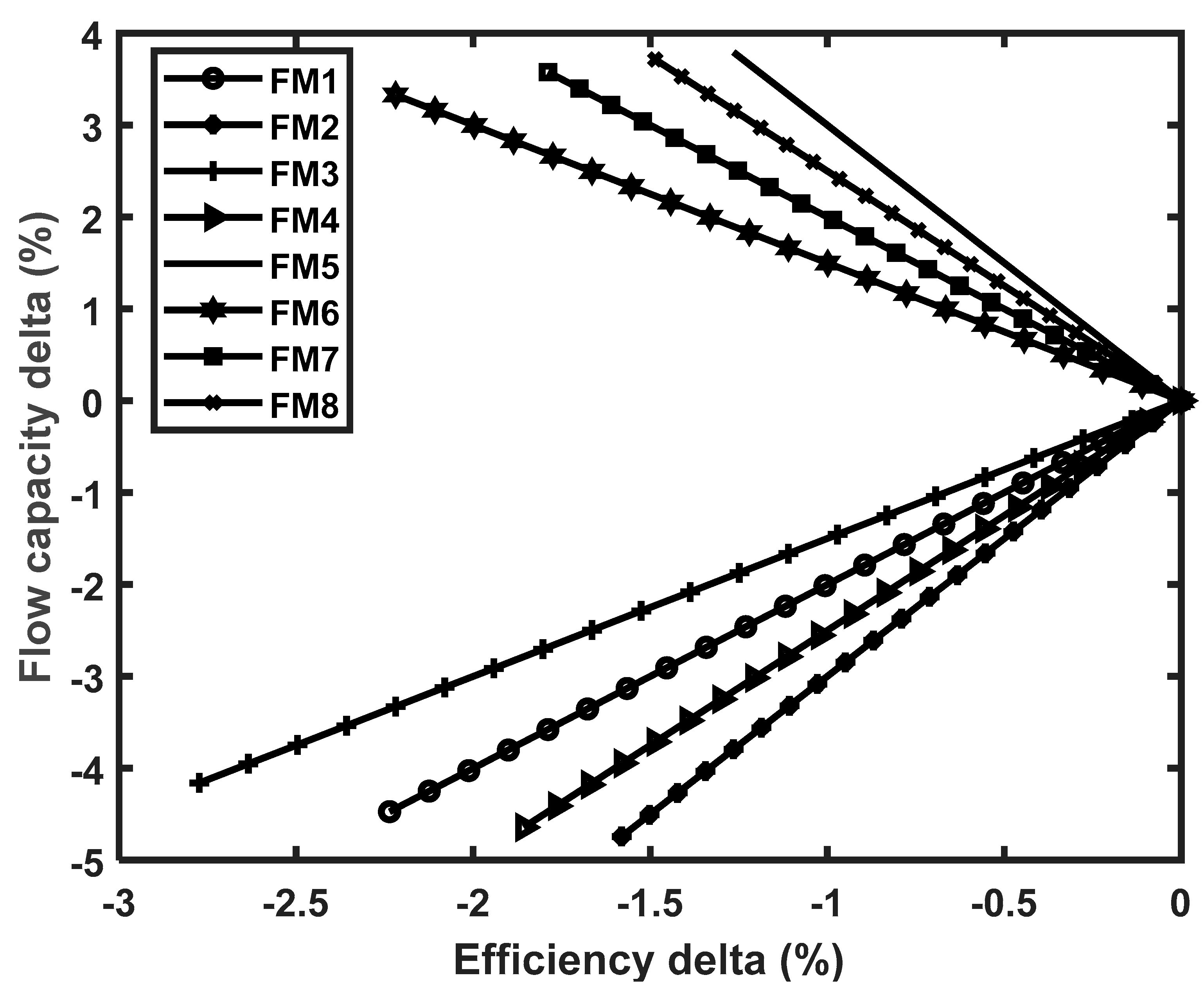
The generalization performance of the CNN and LSTM algorithms was also assessed and compared based on extrapolation data to ensure the stability of the models. The extrapolation data in this case represent performance data of the engine that are not part of the 176,940 datasets. Figure 13 illustrates the fault patterns used to generate the 176,940 data (FM1 and FM2) and the extrapolation data (FM3 to FM8). FM1 refers to the fault magnitude used for the FAN, IPC, and HPC and FM2 for the HPT, IPT, and LPT based on a 2:1 ratio between flow capacity and efficiency changes. Although the 2:1 ratio is the common practice in gas turbine diagnostics [39], this does not seem to be the only possible scenario occurring, according to the reports on gas turbine degradation [1]. Hence, in order to evaluate the influence of the ratio change on the diagnostic accuracy, 3:1, 2.25:1, and 3:2 ratios were considered to generate the extrapolation data.
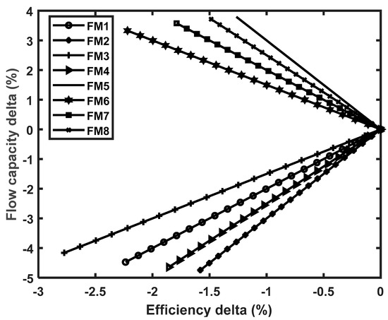
Figure 13.
Flow capacity to efficiency health parameter adjustment.
For the FAN, IPC, and HPC faults, both flow capacity and efficiency values reduced, as seen in the patterns below the zero axis. For the HPT, IPT, and LPT faults, flow capacity increased while efficiency decreased (i.e., the patterns above the zero axis). Module faults are represented in terms of the root sum square of the two performance parameters.
Since the four LSTM models used in the comparative analysis showed similar accuracy, only the results obtained from the ULSTM algorithm are included in Table 17, due to the space limitation. It is seen that the CNN classifiers had better generalization performance than the LSTM classifiers. When the extrapolation data were used, the single-fault classification accuracy and double-fault classification accuracy of the CNN algorithm reduced by 1.8% and 2.8%, respectively. However, the higher than 96% accuracy achieved for both single- and double-component fault classification was in the acceptable performance range to determine the type of the fault that the gas turbine engine had encountered.
Table 17.
Comparison results based on the extrapolation data.
5. Conclusions and Future Work
An adaptive performance-model-assisted deep-convolutional-neural-network method was presented for three-shaft turbofan engine fault diagnostics. The adaptive scheme was applied to track the performance parameter deterioration profiles of the engine gas path and generate fault signatures. A group of deep convolutional neural network modules was integrated to hierarchically detect rapid and persistent faults and isolate the underlying faults, using the fault signatures generated by the adaptive scheme. The performance of the method proposed was evaluated based on a variety of single- and multiple-fault scenarios, and over 96% detection and isolation accuracies were achieved. This reveals the potential of convolutional neural networks to effectively detect and isolate both single and multiple gas path faults. Moreover, the method proposed was compared with two alternative methods, clearly showing that it outperformed both methods. In the future, the authors would like to extend the application of this method for sensor fault/failure detection and isolation and missing sensor replacement purposes. Additionally, the effects of flight-to-flight operating condition variations and engine-to-engine manufacturing tolerances will be analyzed.
Author Contributions
Conceptualization, A.D.F., V.Z., and K.K.; methodology, A.D.F., V.Z., and K.K.; formal analysis, A.D.F.; writing—original draft preparation, A.D.F.; writing—review and editing, A.D.F., V.Z. and K.K.; project administration, K.K. All authors have read and agreed to the published version of the manuscript.
Funding
This research was funded by the Swedish Knowledge Foundation (KKS) under the project PROGNOSIS, Grant Number 20190994.
Institutional Review Board Statement
Not applicable.
Informed Consent Statement
Not applicable.
Data Availability Statement
Not applicable.
Conflicts of Interest
The authors declare no conflict of interest.
References
- Fentaye, A.D.; Baheta, A.T.; Gilani, S.I.; Kyprianidis, K.G. A Review on Gas Turbine Gas-Path Diagnostics: State-of-the-Art Methods, Challenges and Opportunities. Aerospace 2019, 6, 83. [Google Scholar] [CrossRef] [Green Version]
- Li, Y.G. Gas Turbine Performance and Health Status Estimation Using Adaptive Gas Path Analysis. J. Eng. Gas Turbines Power 2010, 132, 041701. [Google Scholar] [CrossRef]
- Mathioudakis, K.; Kamboukos, P. Assessment of the Effectiveness of Gas Path Diagnostic Schemes. J. Eng. Gas Turbines Power 2006, 128, 57–63. [Google Scholar] [CrossRef]
- Lu, F.; Gao, T.; Huang, J.; Qiu, X. A novel distributed extended Kalman filter for aircraft engine gas-path health estimation with sensor fusion uncertainty. Aerosp. Sci. Technol. 2019, 84, 90–106. [Google Scholar] [CrossRef]
- Pourbabaee, B.; Meskin, N.; Khorasani, K. Sensor Fault Detection, Isolation, and Identification Using Multiple-Model-Based Hybrid Kalman Filter for Gas Turbine Engines. IEEE Trans. Control. Syst. Technol. 2016, 24, 1184–1200. [Google Scholar] [CrossRef] [Green Version]
- Loboda, I.; Robles, M.A.O. Gas Turbine Fault Diagnosis Using Probabilistic Neural Networks. Int. J. Turbo Jet-Engines 2015, 32, 175–191. [Google Scholar] [CrossRef]
- Ogaji, S.O.; Singh, R. Advanced engine diagnostics using artificial neural networks. Appl. Soft Comput. 2003, 3, 259–271. [Google Scholar] [CrossRef]
- Fu, X.; Luo, H.; Zhong, S.; Lin, L. Aircraft engine fault detection based on grouped convolutional denoising autoencoders. Chin. J. Aeronaut. 2019, 32, 296–307. [Google Scholar] [CrossRef]
- Li, Y.-G. Diagnostics of power setting sensor fault of gas turbine engines using genetic algorithm. Aeronaut. J. 2017, 121, 1109–1130. [Google Scholar] [CrossRef] [Green Version]
- Mohammadi, E.; Montazeri-Gh, M. A fuzzy-based gas turbine fault detection and identification system for full and part-load performance deterioration. Aerosp. Sci. Technol. 2015, 46, 82–93. [Google Scholar] [CrossRef]
- Romessis, C.; Mathioudakis, K. Bayesian Network Approach for Gas Path Fault Diagnosis. ASME. J. Eng. Gas Turbines Power 2006, 128, 64–72. [Google Scholar] [CrossRef]
- Lee, Y.K.; Mavris, D.N.; Volovoi, V.V.; Yuan, M.; Fisher, T. A Fault Diagnosis Method for Industrial Gas Turbines Using Bayesian Data Analysis. J. Eng. Gas Turbines Power 2010, 132, 041602. [Google Scholar] [CrossRef]
- Chen, H.; Jiang, B.; Ding, S.X.; Huang, B. Data-Driven Fault Diagnosis for Traction Systems in High-Speed Trains: A Survey, Challenges, and Perspectives. IEEE Trans. Intell. Transp. Syst. 2020, 1–17. [Google Scholar] [CrossRef]
- Marinai, L.; Probert, D.; Singh, R. Prospects for aero gas-turbine diagnostics: A review. Appl. Energy 2004, 79, 109–126. [Google Scholar] [CrossRef]
- Pang, S.; Li, Q.; Feng, H. A hybrid onboard adaptive model for aero-engine parameter prediction. Aerosp. Sci. Technol. 2020, 105, 105951. [Google Scholar] [CrossRef]
- Xu, M.; Wang, J.; Liu, J.; Li, M.; Geng, J.; Wu, Y.; Song, Z. An improved hybrid modeling method based on extreme learning machine for gas turbine engine. Aerosp. Sci. Technol. 2020, 107, 106333. [Google Scholar] [CrossRef]
- Zagorowska, M.; Spüntrup, F.S.; Ditlefsen, A.-M.; Imsland, L.; Lunde, E.; Thornhill, N.F. Adaptive detection and prediction of performance degradation in off-shore turbomachinery. Appl. Energy 2020, 268, 114934. [Google Scholar] [CrossRef]
- Losi, E.; Venturini, M.; Manservigi, L.; Ceschini, G.F.; Bechini, G. Anomaly Detection in Gas Turbine Time Series by Means of Bayesian Hierarchical Models. J. Eng. Gas Turbines Power 2019, 141, 111019. [Google Scholar] [CrossRef]
- Tsoutsanis, E.; Hamadache, M.; Dixon, R. Real Time Diagnostic Method of Gas Turbines Operating Under Transient Conditions in Hybrid Power Plants. J. Eng. Gas Turbines Power 2020, 142, 101002. [Google Scholar] [CrossRef]
- Yan, W.; Yu, L. On accurate and reliable anomaly detection for gas turbine combustors: A deep learning approach. arXiv 2019, arXiv:1908.09238. [Google Scholar]
- Fu, S.; Zhong, S.; Lin, L.; Zhao, M. A re-optimized deep auto-encoder for gas turbine unsupervised anomaly detection. Eng. Appl. Artif. Intell. 2021, 101, 104199. [Google Scholar] [CrossRef]
- Ning, S.; Sun, J.; Liu, C.; Yi, Y. Applications of deep learning in big data analytics for aircraft complex system anomaly detection. Proc. Inst. Mech. Eng. Part O J. Risk Reliab. 2021, 235, 923–940. [Google Scholar] [CrossRef]
- Zhou, H.; Ying, Y.; Li, J.; Jin, Y. Long-short term memory and gas path analysis based gas turbine fault diagnosis and prognosis. Adv. Mech. Eng. 2021, 13, 168781402110377. [Google Scholar] [CrossRef]
- Jiao, J.; Zhao, M.; Lin, J.; Liang, K. A comprehensive review on convolutional neural network in machine fault diagnosis. Neurocomputing 2020, 417, 36–63. [Google Scholar] [CrossRef]
- Palazuelos, A.R.-T.; Droguett, E.L.; Pascual, R. A novel deep capsule neural network for remaining useful life estimation. Proc. Inst. Mech. Eng. Part O J. Risk Reliab. 2020, 234, 151–167. [Google Scholar] [CrossRef]
- Li, X.; Ding, Q.; Sun, J.-Q. Remaining useful life estimation in prognostics using deep convolution neural networks. Reliab. Eng. Syst. Saf. 2018, 172, 1–11. [Google Scholar] [CrossRef] [Green Version]
- Wen, L.; Dong, Y.; Gao, L. A new ensemble residual convolutional neural network for remaining useful life estimation. Math. Biosci. Eng. 2019, 16, 862–880. [Google Scholar] [CrossRef] [PubMed]
- Liu, J.; Liu, J.; Yu, D.; Kang, M.; Yan, W.; Wang, Z.; Pecht, M.G. Fault Detection for Gas Turbine Hot Components Based on a Convolutional Neural Network. Energies 2018, 11, 2149. [Google Scholar] [CrossRef] [Green Version]
- Guo, S.; Yang, T.; Gao, W.; Zhang, C. A Novel Fault Diagnosis Method for Rotating Machinery Based on a Convolutional Neural Network. Sensors 2018, 18, 1429. [Google Scholar] [CrossRef] [PubMed] [Green Version]
- Zhao, J.; Li, Y.G. Abrupt Fault Detection and Isolation for Gas Turbine Components Based on a 1D Convolutional Neural Network Using Time Series Data. In Proceedings of the AIAA Propulsion and Energy 2020 Forum, Anaheim, CA, USA, 24–28 August 2020; p. 3675. [Google Scholar] [CrossRef]
- Zhong, S.-S.; Fu, S.; Lin, L. A novel gas turbine fault diagnosis method based on transfer learning with CNN. Measurement 2019, 137, 435–453. [Google Scholar] [CrossRef]
- Yang, X.; Bai, M.; Liu, J.; Liu, J.; Yu, D. Gas path fault diagnosis for gas turbine group based on deep transfer learning. Measurement 2021, 181, 109631. [Google Scholar] [CrossRef]
- Simon, D.L.; Borguet, S.; Léonard, O.; Zhang, X. (Frank) Aircraft Engine Gas Path Diagnostic Methods: Public Benchmarking Results. J. Eng. Gas Turbines Power 2014, 136, 041201. [Google Scholar] [CrossRef] [Green Version]
- Tang, S.; Tang, H.; Chen, M. Transfer-learning based gas path analysis method for gas turbines. Appl. Therm. Eng. 2019, 155, 1–13. [Google Scholar] [CrossRef]
- Hepperle, N.; Therkorn, D.; Schneider, E.; Staudacher, S. Assessment of Gas Turbine and Combined Cycle Power Plant Performance Degradation. In Proceedings of the ASME 2011 Turbo Expo: Turbine Technical Conference and Exposition, Vancouver, BC, Canada, 6–10 June 2011; Volume 54648, pp. 569–577. [Google Scholar] [CrossRef]
- Marinai, L.; Singh, R.; Curnock, B.; Probert, D. Detection and prediction of the performance deterioration of a turbo-fan engine. In Proceedings of the International Gas Turbine Congress, Tokyo, Japan, 2–3 November 2003; pp. 2–7. [Google Scholar] [CrossRef]
- Litt, J.S.; Parker, K.I.; Chatterjee, S. Adaptive gas turbine engine control for deterioration compensation due to aging. In Proceedings of the 16th International Symposium on Air Breathing Engines, Cleveland, OH, USA, 31 August–5 September 2003. ISABE-2003–1056, NASA/TM-2003–212607. [Google Scholar]
- Meher-Homji, C.B.; Bromley, A. Gas Turbine Axial Compressor Fouling and Washing. In Proceedings of the 33rd Tur-Bomachinery Symposium, A&M University, Turbomachinery Laboratories, College Station, TX USA, 21–23 September 2004; pp. 251–252. [Google Scholar]
- Simon, D.L. Propulsion Diagnostic Method Evaluation Strategy (ProDiMES) User’s Guide; NASA/TM-2010-215840; National Aeronautics and Space Administration: Washington, DC, USA, 2010.
- Zaccaria, V.; Fentaye, A.D.; Stenfelt, M.; Kyprianidis, K.G. Probabilistic Model for Aero-Engines Fleet Condition Monitoring. Aerospace 2020, 7, 66. [Google Scholar] [CrossRef]
- Zaccaria, V.; Stenfelt, M.; Sjunnesson, A.; Hansson, A.; Kyprianidis, K.G. A Model-Based Solution for Gas Turbine Diagnostics: Simulations and Experimental Verification. In Proceedings of the ASME Turbo Expo 2019: Power for Land, Sea and Air, Phoenix, AZ, USA, 11–15 June 2019. GT2019-90858. [Google Scholar] [CrossRef]
- Volponi, A.J.; Tang, L. Improved Engine Health Monitoring Using Full Flight Data and Companion Engine Information. SAE Int. J. Aerosp. 2016, 9, 91–102. [Google Scholar] [CrossRef]
- Fentaye, A.; Zaccaria, V.; Kyprianidis, K. Discrimination of Rapid and Gradual Deterioration for an Enhanced Gas Turbine Life-cycle Monitoring and Diagnostics. Int. J. Progn. Health Manag. 2021, 12, 3. [Google Scholar] [CrossRef]
- O’Shea, K.; Nash, R. An introduction to convolutional neural networks. arXiv 2015, arXiv:1511.08458. [Google Scholar]
- Volponi, A.J. Gas Turbine Engine Health Management: Past, Present, and Future Trends. J. Eng. Gas Turbines Power 2014, 136, 051201. [Google Scholar] [CrossRef]
- Nair, V.; Hinton, G.E. Rectified linear units improve restricted boltzmann machines. In Proceedings of the 27th International Conference on Machine Learning, Haifa, Israel, 21–24 June 2010; pp. 807–814. [Google Scholar]
- Kingma, D.P.; Ba, J. Adam: A method for stochastic optimization. arXiv 2014, arXiv:1412.6980. [Google Scholar]
- Srivastava, N.; Hinton, G.; Krizhevsky, A.; Sutskever, I.; Salakhutdinov, R. Dropout: A simple way to prevent neural networks from overfitting. J. Mach. Learn. Res. 2014, 15, 1929–1958. [Google Scholar]
- Soibam, J.; Rabhi, A.; Aslanidou, I.; Kyprianidis, K.; Bel Fdhila, R. Derivation and Uncertainty Quantification of a Da-ta-Driven Subcooled Boiling Model. Energies 2020, 13, 5987. [Google Scholar] [CrossRef]
- Khan, S.; Yairi, T. A review on the application of deep learning in system health management. Mech. Syst. Signal Process. 2018, 107, 241–265. [Google Scholar] [CrossRef]
- Kakati, P.; Dandotiya, D.; Pal, B. Remaining Useful Life Predictions for Turbofan Engine Degradation Using Online Long Short-Term Memory Network. In Proceedings of the ASME 2019 Gas Turbine India Conference, Chennai, India, 5–6 December 2019; pp. 2019–2368. [Google Scholar] [CrossRef]
- Lin, L.; Liu, J.; Guo, H.; Lv, Y.; Tong, C. Sample adaptive aero-engine gas-path performance prognostic model modeling method. Knowl. Based Syst. 2021, 224, 107072. [Google Scholar] [CrossRef]
- da Costa, P.R.d.O.; Akcay, A.; Zhang, Y.; Kaymak, U. Attention and long short-term memory network for remaining useful lifetime predictions of turbofan engine degradation. Int. J. Progn. Health Manag. 2019, 10, 034. [Google Scholar] [CrossRef]
- Bai, M.; Liu, J.; Ma, Y.; Zhao, X.; Long, Z.; Yu, D. Long Short-Term Memory Network-Based Normal Pattern Group for Fault Detection of Three-Shaft Marine Gas Turbine. Energies 2020, 14, 13. [Google Scholar] [CrossRef]
- Siami-Namini, S.; Tavakoli, N.; Namin, A.S. The Performance of LSTM and BiLSTM in Forecasting Time Series. In Proceedings of the 2019 IEEE International Conference on Big Data (Big Data), Los Angeles, CA, USA, 9–12 December 2019; pp. 3285–3292. [Google Scholar]
- Anand, A. Unit-14 Accuracy Assessment; IGNOU: New Delhi, India, 2017. [Google Scholar]
- Kyprianidis, K. On Gas Turbine Conceptual Design. Ph.D. Thesis, Cranfield University, Cranfield, UK, 2019. [Google Scholar]
- Kyprianidis, K. An Approach to Multi-Disciplinary Aero Engine Conceptual Design. In Proceedings of the International Symposium on Air Breathing Engines, ISABE 2017, Manchester, UK, 3–8 September 2017. Paper No. ISABE-2017-22661. [Google Scholar]
- Tumer, I.; Bajwa, A. A survey of aircraft engine health monitoring systems. In Proceedings of the 35th Joint Propulsion Conference and Exhibit, Los Angeles, CA, USA, 20–24 June 1999; p. 2528. [Google Scholar]
- Ruder, S. An overview of gradient descent optimization algorithms. arXiv 2016, arXiv:1609.04747. [Google Scholar]
- Lei, S.; Zhang, H.; Wang, K.; Su, Z. How training data affect the accuracy and robustness of neural networks for image classification. In Proceedings of the 2019 International Conference on Learning Representations (ICLR-2019), New Orleans, LA, USA, 6–9 May 2019; pp. 1–14. [Google Scholar]
- Losi, E.; Venturini, M.; Manservigi, L. Gas Turbine Health State Prognostics by Means of Bayesian Hierarchical Models. J. Eng. Gas Turbines Power 2019, 141, 111018. [Google Scholar] [CrossRef]


Publisher’s Note: MDPI stays neutral with regard to jurisdictional claims in published maps and institutional affiliations. |
© 2021 by the authors. Licensee MDPI, Basel, Switzerland. This article is an open access article distributed under the terms and conditions of the Creative Commons Attribution (CC BY) license (https://creativecommons.org/licenses/by/4.0/).