Multi-Domain Informative Coverage Path Planning for a Hybrid Aerial Underwater Vehicle in Dynamic Environments

Abstract

Hybrid aerial underwater vehicles (HAUV) are a new frontier for vehicles. They can operate both underwater and aerially, providing enormous potential for a wide range of scientific explorations. Informative path planning is essential to vehicle autonomy. However, covering an entire mission region is a challenge to HAUVs because of the possibility of a multidomain environment. This paper presents an informative trajectory planning framework for planning paths and generating trajectories for HAUVs performing multidomain missions in dynamic environments. We introduce the novel heuristic generalized extensive neighborhood search GLNS–k-means algorithm that uses k-means to cluster information into several sets; then through the heuristic GLNS algorithm, it searches the best path for visiting these points, subject to various constraints regarding path budgets and the motion capabilities of the HAUV. With this approach, the HAUV is capable of sampling and focusing on regions of interest. Our method provides a significantly more optimal trajectory (enabling collection of more information) than ant colony optimization (ACO) solutions. Moreover, we introduce an efficient online replanning scheme to adapt the trajectory according to the dynamic obstacles during the mission. The proposed replanning scheme based on KD tree enables significantly shorter computational times than the scapegoat tree methods.

1. Introduction

Both unmanned aerial vehicles (UAVs) and unmanned underwater vehicles (UUVs) are widely applied in civil and military fields. However, a single UAV or UUV cannot go on multidomain missions, such as mapping of isolated water regions, multidomain oceanic monitoring, and inspections of submersed structures and ship hulls [1]. As a result, a hybrid aerial underwater vehicle (HAUV) that can operate both underwater and aerially would be helpful to accomplish such tasks. Thus, interest has risen in HAUVs.

In recent years, HAUV research has focused more on two subsets of HAUV: HAUVs based on fixed-wing or rotary-wing UAVs combined with UUVs’ underwater functionality. Weisler et al. first achieved aerial flight, underwater cruising, and cross-domain transition with one vehicle [2]. Later, Stewart et al.’s work added an aft water rotor to optimize underwater motion on multi-domain missions [3]. As for rotary-wing HAUVs, which have shown good control potential for multidomain emissions, they were first put forward by Drews et al. in 2014 [4]. Later, some works combined rotary-wing UAVs with underwater rotors to allow underwater operation [5,6,7]. These HAUVs showed controllable and smooth operation; nevertheless, they are limited by their UAV-based structures. Our previous work was inspired by gliders, which have proven to be the most efficient UUVs [8]. Our HAUV was a combination of underwater gliders (UGs) and UAVs. We showed the functionality of underwater gliders in both vertical and level flight.

Many works on HAUV have been performed recently. However, most of them focus on the control system and structural design. Few studies on path planning for HAUVs in multidomain environments have been proposed. These vehicles have different work modes in various domains, and are supposed to conform to various constraints in different environments. Therefore, they require copmlex path planning and trajectory generation strategies compared to other vehicles, such as UAVs and USVs. Indeed, the trajectory planning for HAUV is of great significance. Therefore, we propose a way to grasp and cluster the information from the environment and find an energy-saving mission trajectory for an HAUV.

1.1. Informative Path Planning

The developing requirements of robot monitoring have given rise to the challenge that the equipped devices are subject to limited resources, such as mission time and energy. Therefore path planning for vehicles to maximize the information gathered is of significance. In the aerial environment, many works have been done to maximize information gathering. 2D spaces were divided into several cells to find solutions for coverage paths in [9,10]. The cells can be trapezoidal or boustrophedon [11,12,13]. Finding the shortest and most efficient sequence of cell visiting, and generalizing the path, was proven to be NP-hard and was formulated as a TSP problem by Lewis et al. [14]. Vandermeulen et al.’s work [15] decomposed the environment into ranks. They solved multiple TSP problems on the ranks to minimize the number of turns taken by robots, which relates to the mission time. Tokekar and Yu reduced the problem to a generalized traveling salesman problem (GTSP). They could obtain optimal solutions in reasonable durations. They also proposed a strategy with which to recharge UAVs by UGVs during flight [16]. Their former work proved the GTSP solver GLNS performs better in terms of speed and path generation than other TSP solvers [17]. Our former studies [18,19,20,21,22,23,24] involved a lot of research on path planning in underwater and sea surface cases. Concerning the sea surface, Yuanchang Liu et al.’s work [25,26,27] presents several algorithms for single and multiple unmanned surface vehicles. Ref. [28] proposed a dive planning method to monitor underwater environments. Hollinger et al. [29] proposed a method to efficiently inspect underwater structures using AUV, based on Bayesian active learning. Cao et al. [30] presented a method to decompose the environment into several subspaces and solve the problem in two levels: sequence of subspace visiting and detailed coverage in subspaces. To efficiently grasp information from the environment, Jing. et al. [31] directly planned and optimized paths via a video stream gathered by a UAV. Vidal E. et al. proposed a novel algorithm based on Octree to achieve full coverage of unknown environments [32]. In [33], Zacchin L. et al. proposed a sensor-driven, two-level seabed path planning solution for AUV, which is available for any acoustic or optical sensor. In [34], Paull L. et al. presented a method that was combined with a new concept coined branch entropy based on hexagonal cell decomposition to achieve efficient multi-objective optimization.

However, the operating environment for an HAUV is simple neither underwater nor aerially. We consider the surroundings of the HAUV to be simple in 3D when few obstacles exist in the environment, and safety constraints mainly come from the terrain. Considering a multidomain mission for an HAUV, simple path planning is not sufficient. In addition, some constraints should be set according to the HAUV’s motion capabilities. Considering the motion capabilities of a UAV, Kumar and Mellinger developed an algorithm to minimize the fourth derivation of a position function (snap). They reduced the cost of a flight and could satisfy constraints on safety, velocity, and acceleration as well [35]. Based on the snap minimizing methods, Chen set collision-free flight corridors and generated trajectories in corridors to ensure flight safety [36]. Similarly, Gao et al.’s work set corridors for UAVs, but with a fast marching-based method. They also used a Bernstein polynomial to represent trajectories piecewise [37]. Gregory Hitz et al. [38] proposed a CIPP algorithm that optimizes a parametrized path in continuous space.

All the previous works we mentioned focused on UUVs and UAVs operating with simple domain path planning. However, multidomain missions such as mapping isolated water regions and inspecting submersed structures bring challenges to such vehicles. A heterogeneous vehicle team of a UAV and a UUV is currently used to accomplish the multidomain tasks according to [39]. However, this kind of strategy is expensive and inefficient [40]. Therefore, a framework of information clustering, path planning, and trajectory generation for HAUVs, which are capable of operating well both in the air and underwater, will be helpful for multidomain missions.

1.2. Path Planning with Unknown Obstacles

Aside from the planned path for a HAUV, some unknown obstacles, such as animals, floating trash, and branches, could appear in real-time missions. As a consequence, a path replanning method is a requirement for an HAUV path planning framework. To replan a path, searching for a new collision-free spot near the obstacle in question and inserting it into the original path would be helpful. Finding nearby collision-free spots can be generalized as a k-nearest neighbors (KNN) problem. Our method solves the problem by reducing the KNN to a nearest neighbor search (NNS). The concept of KNN was firstly presented by Fix and Hodges in 1951 [41]. Later, KNN was widely used in data mining, computer version, agriculture, etc. Many studies have been performed to prove the efficiency of the results of KNN algorithms [42,43,44]. When reduced to NNS, solutions are mainly based on three methods: space segmentation, hash algorithm, and graph theory. Space segmentation by trees and cluster algorithms perform well. A KD tree can be quickly constructed and used to search for a target ($O\left(logN\right)$) [45,46], but inserting new elements into a KD tree may lead to unbalance. Cluster algorithms, k-means, GNAT, the anchor hierarchy, the cover tree, and spill-tree have been used to solve that problem, but these algorithms did not show decisive advantages over search trees [47]. In 1998, Indyk and Motwani presented LSH (locality sensitive hashing) [48], which can be used to cope with tremendous data. In recent years, many studies based on graph theory have been performed. Jing et al. [49] built a neighborhood graph for data subsets to achieve efficient and accurate KNN graph construction.

1.3. Contributions

This paper proposes a method to gather information from a given environment and find an energy-saving mission trajectory for the HAUV to cover this target space. The core contributions of this work are:

• Presenting a framework of multidomain path planning for HAUVs, including information clustering, path planning trajectory generation, and unknown obstacle avoidance in static environments and environments with current fields.
• Addressing a heuristic algorithm with a weighted edge for multidomain path planning based on general large neighborhood searching and k-means.
• Presenting a trajectory generation method combining B-spline with KD tree. The output trajectory is ensured to be smooth and safe, and conform to different constraints, underwater or aerial.
• Presenting a method to avoid random unknown obstacles based on the scapegoat tree and KD tree.

The remainder of this paper is organized as follows: Section 2 formulates the mathematical models and presents the theory of path planning, replanning, and trajectory generation methods. Section 3 gives a detailed description of the path planning and replanning algorithm. In Section 4, the trajectory generation scheme is outlined. The experimental results and discussion is proposed in Section 5. Finally, in Section 6 our findings are concluded, and avenues of future work are presented. The mathematical symbols denoted in this paper are as summarized in Table 1.

Table 1. Nomenclature.

Variable	Description	Variable	Description
P	The whole path.	$\mathsf{\Phi }\left\{p_1,p_2,\dots p_i,\dots ,p_n\right\}$	$\mathsf{\Phi }$ is denoted as the set of target spots the while $p_i$ is coordinate of the $i_{th}$ target spot in path.
$sub{P}_i$	The $i_{th}$ sub path in P, each sub path contains 5–10 path segment, which denote the length of path the HAUV can detect when path re-planning.	${\mathsf{\Gamma }}_i$	The path segment between $p_i$ and $p_{i+1}$.
$D_i$	The length of ${\mathsf{\Gamma }}_i$.	${\xi }_i$	The overall weighted edge of $i_{th}$ path segment.
${\xi }_{surf/air/sea/c}$	The overall weighted edge of surface/air/water/current fields.	$v_i$	The velocity with which HAUV move from $p_i$ to $p_{i+1}$.
$a_i$	The acceleration with which HAUV move from $p_i$ to $p_{i+1}$.	$v_{max}^i$	The maximum velocity with which HAUV move from $p_i$ to $p_{i+1}$.
$a_{max}^i$	The maximum acceleration with which HAUV move from $p_i$ to $p_{i+1}$.	$OBS\left\{ob{s}_1,ob{s}_2,\dots ,ob{s}_k\right\}$	$OBS$ is the set of randomly appeared unknown obstacles, and $ob{s}_j$ is the set of all spots’ coordinate of the $j_{th}$ obstacle.
$ob{s}_j\left\{ob{s}_j^1,ob{s}_j^2,\dots ,ob{s}_j^q\right\}$	Coordinate of all the spots in the $j_{th}$ obstacle.	$CI{R}_s^1/SP{H}_s^1$	The minimum circumscribed circle/sphere of $ob{s}_s$.
$CI{R}_s^2/SP{H}_s^2$	The collision free circle/sphere out of $ob{s}_s$, which is an extension of $CI{R}_s^1/SP{H}_s^1$	$D_{obs}^j$	The shortest distance between the obstacle ${obs}_s$ and ${SPH}_s^2$.
$D_{mi}$	The minimum distance between $P_{m+i}$ and $ob{s}_s$.	$tertree$	KD-tree constructed by terrain map.
$obtree$	KD-tree constructed by obstacles.	$F_t^{x,y,z}$	The function of trajectory.
$\alpha$	The control parameter of scapegoat tree.	$TE$	The spots set of terrain map. (The barriers.)
$\mathsf{\Omega }\left\{s_1,s_2,\dots ,s_m\right\}$	$\mathsf{\Omega }$ is denoted as map of informative spots while $\left\{s_1,s_2,\dots ,s_m\right\}$ are the coordinates of those spots.	$Y_{air/sea}$	The force HAUV need to overcome without current fields.
$Y_{airc/seac}$	The force HAUV need to overcome with current fields.	$v_c$	The velocity of currents.
$S_{air}$	wing area of the HAUV.	${\rho }_{air/sea}$	Density of air/sea water.
$C_{air/sea}$	Coefficient of lift/fraction in air/sea water.	$ve{h}_L$	The length of HAUV.
$CO{V}_i$	The covariance of the $i_{th}$ informative spots group.	$e_{x,y,z}$	The expectation of the $i_{th}$ informative spots group.
$x_{max}/y_{max}/h_{max}$	The size of terrain map in simulation.	$\eta$	The control parameter of current fields checking.

2. Problem Formulation

In this paper, we address the problem of multidomain path planning and trajectory generation. We consider the cases of an HAUV moving underwater, aerially, and between the two media (water and air). The vehicle is required to follow a low-cost, safe, and smooth trajectory within its motion capabilities when random obstacles and disruptions exist.

For n clusters of information spots, our goal is to pick one target spot from each group, and minimize the energy cost for all spots traversed. The whole mission is required to conform to all constraints in static and dynamic environments, and the HAUV’s motion capabilities. We divide the operation modes of each path segment ${\mathsf{\Gamma }}_i$ between $p_i$ and $p_{i+1}$ into three modes according to the specific environment the trip involves.

In each mode, we set weighted edge ${\xi }_i$, to describe the energy cost per meter during the mission. Our goal is to minimize the cost of the whole path and then generate a smooth, safe trajectory that conforms to velocity and acceleration constraints in both static and dynamic environments. Let the obstacles in the environment be $OBS$; let $F_t^{x,y,z}$ be the output trajectory. Let $D_i$ be the distance of the path segment between target spot $p_i$ and $p_{i+1}$. The problem can be generalized as in Equation (1):

$$\begin{array}{ccc}\hfill & \mathbf{minimize}:\hfill & \hfill \sum _{i=1}^{n-1}{\xi }_i{D}_i\\ \hfill & \mathbf{s}.\mathbf{t}.:\hfill & \hfill v_i\le v_{max}^i\\ \hfill & \hfill & \hfill a_i\le a_{max}^i\\ \hfill & \hfill & \hfill F_j^{x,y,z}\cap OBS=⌀\\ \hfill & \hfill & \hfill F_j^{x,y,z}\cap TE=⌀\end{array}$$

(1)

Figure 1 gives an example of a path segment within a whole path:

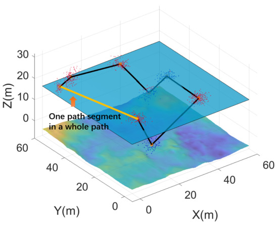
Figure 1. The path segment will be weighted according to the environment.

Along each path segment ${\mathsf{\Gamma }}_i$, the HAUV should move with the corresponding maximum velocity and acceleration. Additionally, the final output trajectory $F_t^{x,y,z}$ should be free from obstacle spots, which contain the unknown obstacles $OBS$ and terrain barriers $TE$.

2.1. Motion and Structural Parameters of the HAUV

The HAUV discussed in our work is an integration of fixed-wing UAVs, rotary-wing UAVs, and UGs [8]. Details are illustrated in Figure Figure 2. The mass of the HAUV is 15 kg, each wing is 750 mm * 300 mm, and the length of the glider is 1000 mm. The main structures of the HAUV are fixed wings, rotary wings, and a waterproof container.

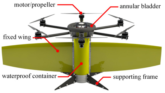
Figure 2. A 3D rendering of the proposed HAUV integrating the features of fixed-wing UAVs, rotary-wing UAVs, and UGs [8].

Since the HAUV can move both underwater and aerially, the motion modes of the HAUV can be divided into three categories: underwater, aerial, and transitioning (between water and air). Figure 3 illustrates the motion of the HAUV.

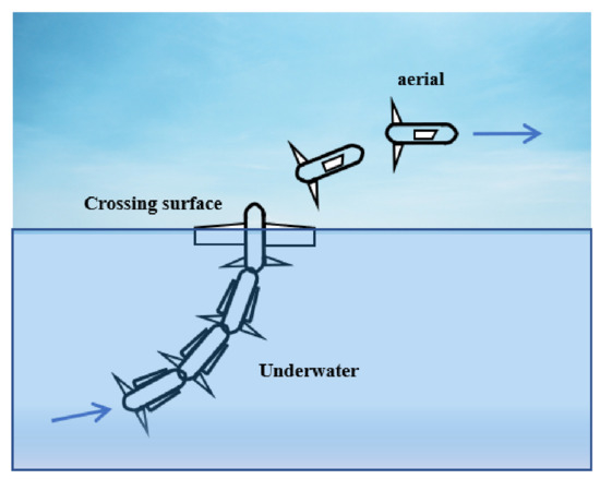
Figure 3. The three mission modes of the HAUV. The edge weight is different per unit of distance for each situation: the fulfill per meter underwater is 5 times of that of flying. The motion constraints also vary: the maximum velocities are: 3 m/s underwater, 10 m/s aerially, and 1 m/s while transitioning (between water and air). The accelerations are: $2{\mathrm{m}}^2/\mathrm{s}$ underwater, $3{\mathrm{m}}^2/\mathrm{s}$ aerially, and $1{\mathrm{m}}^2/\mathrm{s}$ while transitioning.

Consider the specific environment of the path between each two spot. The path that the HAUV visits between target spots $p_i$ and $p_{i+1}$ can be divided into four types. The four types of path in Figure 4 are as follows.

1.

Both $p_i$ and $p_{i+1}$ are underwater;

2.

Both $p_i$ and $p_{i+1}$ are aerial;

3.

$p_i$ is underwater but $p_{i+1}$ is aerial;

4.

$p_i$ is aerial but $p_{i+1}$ is underwater.

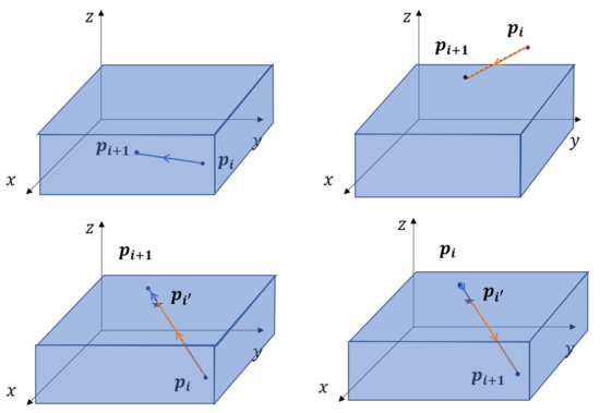
Figure 4. Four types of trip according to the HAUV’s mission mode. A blue arrow illustrates an underwater path, and an orange one means an aerial one. Regarding when the trip crosses domains, the intersection point on surface will be inserted into the target spots set.

As the HAUV has different motion capabilities in diverse mission environments, different dynamic constraints should be set. Considering the experimental data of our former work, NEZHA, in this paper, we roughly define the motion capabilities of the HAUV as follows: The aerial velocity of the HAUV can range from 0 to 10 m/s, and it can range from 0 to 3 m/s under the water. The acceleration can vary from 0 to $3{\mathrm{m}}^2/\mathrm{s}$ aerially, and from 0 to $2{\mathrm{m}}^2/\mathrm{s}$ underwater. In addition, the HUAV can leave the water with a velocity no higher than 1 m/s and acceleration no greater than $1{\mathrm{m}}^2/\mathrm{s}$. Within a fixed period, the HAUV will move from $p_i$ to $p_{i+1}$. The trajectory should conform to motion and space constraints.

2.2. Environmental Settings

2.2.1. Information Spots Cluster

In the real world, most of the informative areas can be detected before the mission, such as those that will be interesting because of chlorophyll and oxygen content. Therefore, in this work, we assume that the informative spots are known, and a randomly set terrain map based on a real-world map denotes the seabed. Let n groups of random spots represent information spots that need to be visited by the HAUV. The HAUV is required to visit one spot that each spots group must visit. An informative spots map $\mathsf{\Omega }$$\left\{s_1,s_2,\dots s_m\right\}$ can be divided into n groups. The process of picking the target spot in each group can be generalized to a GTSP problem. $\mathsf{\Phi }$$\left\{p_1,p_2,\dots ,p_i,\dots p_n\right\}$ of the group $1,2,\dots i,\dots n$. However, the energy cost for each path segment, for every unit of distance, varies with the type of environment and the HAUV’s mission mode. To solve this problem, we determine weights for different path segments, which are set as heuristics.

2.2.2. Unknown Obstacle Avoidance

In practical operations, the HAUV is always subject to finite sensing resources; it cannot monitor the whole path at one time. Therefore, in this work whole path is divided into several subpaths. In the path P$\left\{sub{P}_1,sub{P}_2,\dots ,sub{P}_n\right\}$, each subpath contains more than 5 and less than 10 spots. Within the duration of $sub{P}_i$$\left\{p_m,p_{m+1}\dots ,p_{m+n}\right\}$, randomly shaped obstacles can appear with a certain probability in path segment [$p_{m+i},p_{m+i+1}$]. We regard each obstacle as scattered points, and use k-means to find the center of each obstacle. For obstacles $ob{s}_j$ whose distances to the $sub{P}_i$ are less than the length of the HAUV, collisions happen. All the obstacles can be written as $OBS$$\left\{ob{s}_1,ob{s}_2,\dots ,ob{s}_k\right\}$. For the $j_{th}$ obstacle $ob{s}_j$ in $sub{P}_i$, all points on $ob{s}_j$ are $[ob{s}_j^1,ob{s}_j^2,\dots ob{s}_j^q]$. During the path segment from $p_{m+i}$ to $p_{m+i+1}$, if obstacle $ob{s}_s$ exists, let the farthest distance $r_s^1$ from $[ob{s}_s^1,ob{s}_s^2,\dots ob{s}_s^{k_s}]$ be the radius. Then draw a circle $CI{R}_s^1$, such that $CI{R}_s^1$ is free of obstacles. Then, extend $CI{R}_s^1$ to $CI{R}_s^2$, whose radius is denoted as $r_s^2=ve{h}_L+r_s^1$. Therefore, the space in $CI{R}_s^2$ will be collision-free for the HAUV. The method in a two dimensional environment is as shown in Figure 5. Extended to three dimensions, the strategy also works.

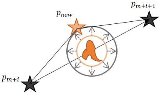
Figure 5. Obstacle avoidance strategy: extend the outer circle of obstacles to $CI{R}_s^2$ and find a free point set on the circle. If there is no solution found, $CI{R}_s^2$ must be extended again.

Finding the free point set on $CI{R}_s^2$ and picking out one to insert into the path can be generalized to a KNN problem—a fixed-radius near neighbors problem: picking one lowest-cost spot from the set and inserting it into the original succession of path spots. If there is no solution on $CI{R}_s^2$, the circle $CI{R}_s^2$ must be extended again such that $r_s^2=ve{h}_L+r_s^2$. In Section 3.2, we present our method to finding a solution.

2.2.3. Dynamic Environment with Current Fields

During operations both aerial and underwater, the HAUV will always face current fields. When in the air, the air drag is normally much weaker than the vehicle’s gravity, so we only consider the lift caused by currents. When there are currents, the lift force is as in the following Equation (2):

$$\begin{array}{c}\hfill Y_{airc}=1/2\ast {\rho }_{air}\ast C_{air}\ast S_{air}\ast {(v_i+v_c)}^2\end{array}$$

(2)

When the HAUV moves in a static environment, the lift force is as in Equation (3):

$$\begin{array}{c}\hfill Y_{air}=1/2\ast {\rho }_{air}\ast C_{air}\ast S_{air}\ast v_i^2\end{array}$$

(3)

where $Y_{air/airc}$ denotes the lift force when the HAUV is in the static environment or current field, and $v_i$ defines the velocity of the HAUV in ${\mathsf{\Gamma }}_i$, which is expressed in m/s. ${\rho }_{air}$ is the air density, affected by altitude. $S_{air}$ is the reference area or the wing area of an aircraft measured in square meters, and $C_{air}$ is the coefficient of lift, depending on the angle of attack and the type of airfoil. We roughly set $C_{air}$ as 1 and ${\rho }_{air}$ as $1.2{\mathrm{kg}/\mathrm{m}}^3$. When there are no current fields, $v_i$ is the average velocity during the HAUV mission. When currents exists, $v=v_i+v_c$, where $v_c$ refers to the currents velocity. The size of our HAUV’s wing area on each side is 750 mm * 300 mm; therefore, the $S_{air}$ can be roughly set to 0.1–0.225 according to the direction of currents.

Likely, in an underwater environment, the power generated by the propeller needs to overcome the lift and frictional resistance. From our experimental data, for most scenarios, the lift is much more than resistance, so we only consider the lift and roughly regard the influence of current in as Equation (4):

$$\begin{array}{c}\hfill Y_{seac}=1/2\ast {\rho }_{sea}\ast C_{sea}\ast S_{sea}\ast {(v_i+v_c)}^2\\ \hfill Y_{sea}=1/2\ast {\rho }_{sea}\ast C_{sea}\ast S_{sea}\ast v_i^2\end{array}$$

(4)

where the ${\rho }_{sea}$ is $1205{\mathrm{kg}/\mathrm{m}}^3$, $S_{sea}$ is $0.33{\mathrm{m}}^2$, and $C_{sea}$ depends on the current fields and the HAUV’s velocity, we calculate it bt ITTC recommend formula (5), where $Re$ is the Reynolds number. In Section 3.1 and Section 3.2 we will discuss the method to measure the influences of currents and the solution to avoid them.

$$\begin{array}{c}\hfill C_{sea}=\frac{0.075}{{(lgRe-2)}^2}\end{array}$$

(5)

3. Multi-Domain Informative Path Planning

The framework of the whole algorithm is shown in Figure 6. The input the presented framework is scattered informative spots. Through the heuristic GLNS and k-means solver, the spots are clustered, and the path planning is described in Section 3.1. Then in Section 3.2, whether unknown obstacles exist is solved, and replanning is explained for path segments that pass obstacles. The trajectory regeneration based on that path found in the former section is explained as well.

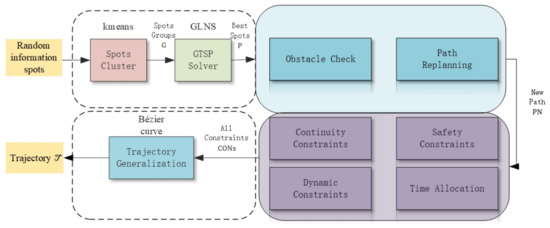
Figure 6. The framework of the whole algorithm. The inputs of this system are randomly created information spots, obstacle sets, and current fields. The output is a smooth, safe, low-cost trajectory conforming to all constraints.

To simulate the target motion space, we can randomly create m spots. Both the number of spots and the positions must conform to a Gaussian distribution. When passing through the target space, the HAUV has to sample or move to some spot of scientific relevance. Therefore, a target spot should be selected from all the information spots. Since all the terrain map is fixed, KD tree $treTree$ stores the environmental information to enable quick reactions to the NNS problem. An example of this information mapping is in Figure 7.

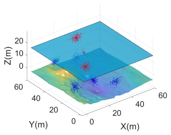
Figure 7. Randomly generated information spots. Through KMEANS (MATLAB) the spots were clustered into several sets. The input for ACO is the center of each set, and the input for GLNS is all the clustered spots.

To solve this problem, informative spots are divided into K clusters. K is the number of groups that the HAUV is supposed to visit. We found the solution to our example by using the KMEANS solver in MATLAB. The result returned contains the group number of each spot and the geometric center spots $c_1,c_2,\dots ,c_n$ of each group. Therefore, the problem can be formulated by finding a target spot in each cluster, a GTSP problem.

The GLNS algorithm was presented by Stephen L. Smith and Frank Imeson, based on adaptive large neighborhood searching [50]. They proved that this algorithm is an efficient solver for the GTSP problem [51]. It was confirmed to be efficient at finding solutions to GTSP problems in [16].

In this work, we present a method to calculate the energy costs that the HAUV incurs in different environments based on the 3D Euclidean distance between each pair of target spots, and set a weighted edge for each distance according to the environment via heuristics. Based on the KD tree, we regard the replanning of the path segment as a fixed-radius near neighbors problem. The inputs for our solver are informative spots clusters, and output is the optimal path.

3.1. Path Planning Based on Heuristic GLNS

A brief description of the GLNS algorithm is as follows: The input for GLNS is a weighted graph: $G(V,E,$$\omega$). The graph contains the information of vertices of clusters and edges. Each round of a GLNS search starts with an initial tour which is randomly selected; then a vertex will be inserted according to heuristics. After each iteration, the new tour is accepted or declined based on an annealing criterion, for which either a fixed number of non-improving iterations is run or warm restarts.

In this study, we set heuristics according to the domain such that the HAUV would have minimal energy consumption in the various mission modes. The heuristic GLNS solver was used to find the solution for the optimization problem of the coverage path. Each information spot in the target space corresponded to a vertex. KMEANS cluster solver defined the informative spots. Edges were defined as the Euclidean weighted distances between pairs of spots. The weight of each edge was related to the specific environment. For comparison, a common TSP solver, the ant colony algorithm (ACO), was also used to find target spots with the input of center spots $c_1{,}_2,\dots c_n$.

Recall that for each path segment between $p_i$ and $p_{i+1}$, there are four possible types of mission environment. The energy cost differs when the HAUV is moving underwater, aerially, and transitioning between the two. According to the experimental data, we can assume the energy cost of the HAUV moving underwater is five times that of flying per meter. Let ${\xi }_{sea}$ be the energy weight of the HAUV moving one meter underwater, and ${\xi }_{sea}$ equals 5${\xi }_{air}$. Under such situations, the HAUV can be regarded as a particle, whereas its length $ve{h}_L$ must be considered when it switches medium. Figure 8a,b gives a comparison between an output path with a weighted edge and a path without a weighted edge. In the latter situation, the HAUV may choose a shorter path but with a higher energy cost.

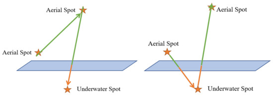
Figure 8. This figure illustrates a comparison between weighted edge and non-weighted edge path generation with the same spots set. The underwater part of the path is orange, and the aerial part is green. Without weighted edges, the HAUV will choose a shorter path that is more energy consuming.

While the HAUV switches transport media, the HAUV will be half underwater and half aerial at a certain point. Therefore, the energy cost weight function can be generalized as Equation (6):

$$\begin{array}{cc}\hfill {\xi }_{surf}& =\frac{\left(\xi \ast \frac{L}{2}+5\xi \ast \frac{L}{2}\right)}{L}\hfill \\ \hfill & =3\xi \hfill \end{array}$$

(6)

For example, to calculate the cost $C_i$ of the trip between $p_i$ and $p_{i+1}$, the first thing is to find the cross point $p_i^{\prime }$. Let $D_i^{air}$ be the distance between $p_i$ and $p_i^{\prime }$, and $D_i^{sea}$ be that of $p_{i+1}$ and $p_i^{\prime }$. The cost in a static environment is calculated as Equation (7):

$$\begin{array}{cc}\hfill C_i& =\left(D_i^{air}-\frac{L}{2}\right)\ast {\xi }_{air}+\frac{L}{2}\ast {\xi }_{surf}+\left(D_i^{sea}-\frac{L}{2}\right)\ast {\xi }_{sea}\hfill \\ \hfill & =D_i^{air}\ast {\xi }_{air}+D_i^{sea}\ast {\xi }_{sea}\hfill \end{array}$$

(7)

Then the cost $C_i$ in a static environment for each spot is put into an iteration cycle of removal and insertion functions in the GLNS solver as a parameter.

As we mentioned in Section 2.2.3, we consider the lift for flight and resistance and lift underwater, based on Equation (2), Equation (3), and Equation (4). We can roughly calculate the weighted edge parameter caused by currents by Equation (8):

$$\begin{array}{c}\hfill \frac{{\xi }_i^{air/water}}{{\xi }_i^c}=\frac{Y_{airc/seac}-Y_{air/sea}}{Y_{air/sea}}\end{array}$$

(8)

We roughly regard both sides of Equation (8) as equal. Therefore, the overall cost function can be written as Equation (9):

$$\begin{array}{cc}\hfill C_i& =D_i^{air}\ast {\xi }_{air}+D_i^{sea}\ast {\xi }_{sea}+D_i\ast {\xi }_c\hfill \end{array}$$

(9)

Given the best path $\mathsf{\Phi }$, if the HAUV is required to stop at a specific location and perform some function, such as sampling, there is no need to generate a smooth trajectory. For each trip, the HAUV only needs to accelerate from 0 m/s with an acceleration equal to $0{\mathrm{m}}^2/\mathrm{s}$. Then, it must slow down to 0 m/s. At each spot, the HAUV can start with an arbitrary angle. Additionally, it should obey the trapezoidal velocity planning strategy to achieve the shortest mission time and lowest energy expenditure.

3.2. Obstacle Avoidance Path Re-Planning

When moving in open areas, the HAUV may encounter some obstacles which cannot be detected beforehand. For example, the trash and creatures in the sea, and birds in air. To take such scenarios into consideration, paths will need to be re-planed. Furthermore, the HAUV should also avoid strong currents. Therefore, we discuss a path replanning method in this section to solve such problems.

3.2.1. Path Replanning in Current Fields

As currents have different directions, their effects on the HAUV’s path can be positive and negative. We firstly calculate the absolute value of current fields per meter of movement. Then its influence (positive or negative) is calculated in regard to the intersection angle ${\beta }_i$ between the current vector and subpath vector. Each subpath between $p_i$ and $p_i+1$ will be traversed by step $j_{x,y,z}$: $\left\{p_i(x_i,y_i,z_i),p_{i+j}(x_i+j_x,y_i+j_y,z_i+j_z),\dots ,p_{i+1}(x_{i+1},y_{i+1},z_{i+1})\right\}$. We use indicator $\eta$ to evaluate the current field. Once ${\xi }_c^{ji}$ is greater than $\eta {\xi }_i$, the weighted edge ${\xi }_c^{ji}$ and coordinate $p_{i+j}$ are recorded as obstacles. The whole framework can be generalized as shown in Figure 9:

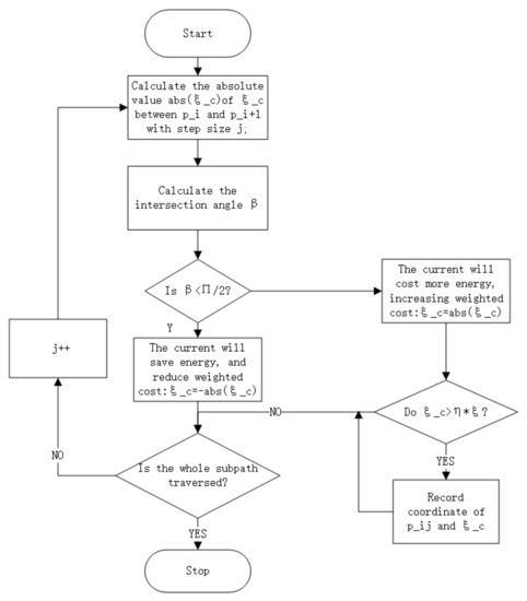
Figure 9. The input of the algorithm is a subpath of the overall path, and the output is the recorded area having strong currents. In the next Section 3.2.2, we discuss the replanning method to avoid the strong currents and obstacles.

3.2.2. Obstacle Avoidance

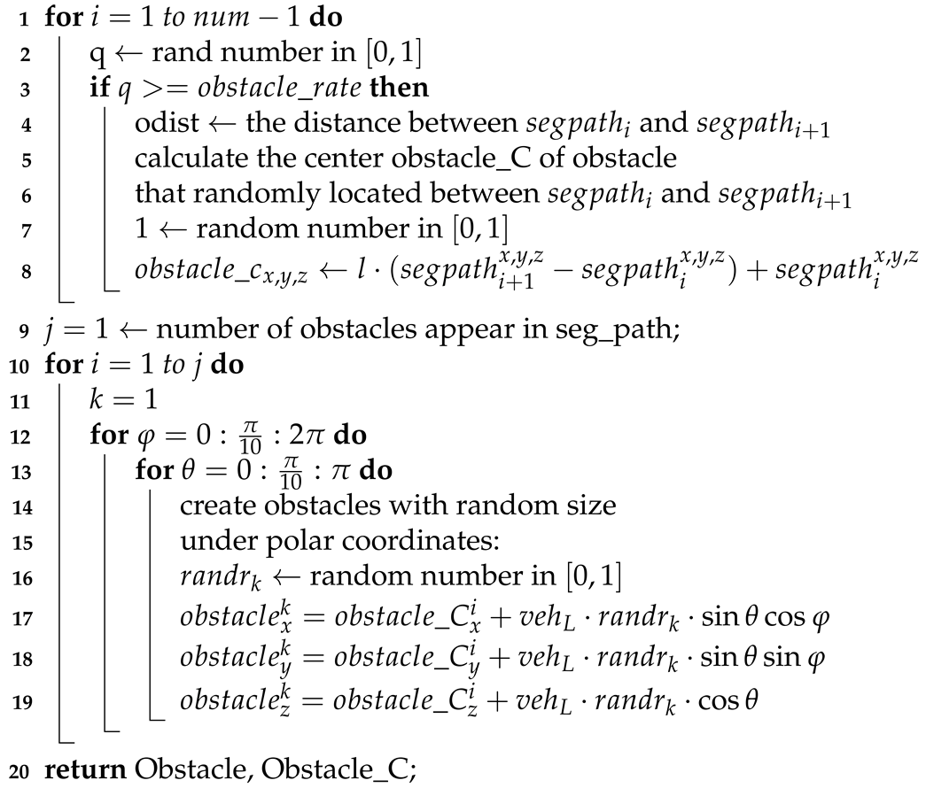
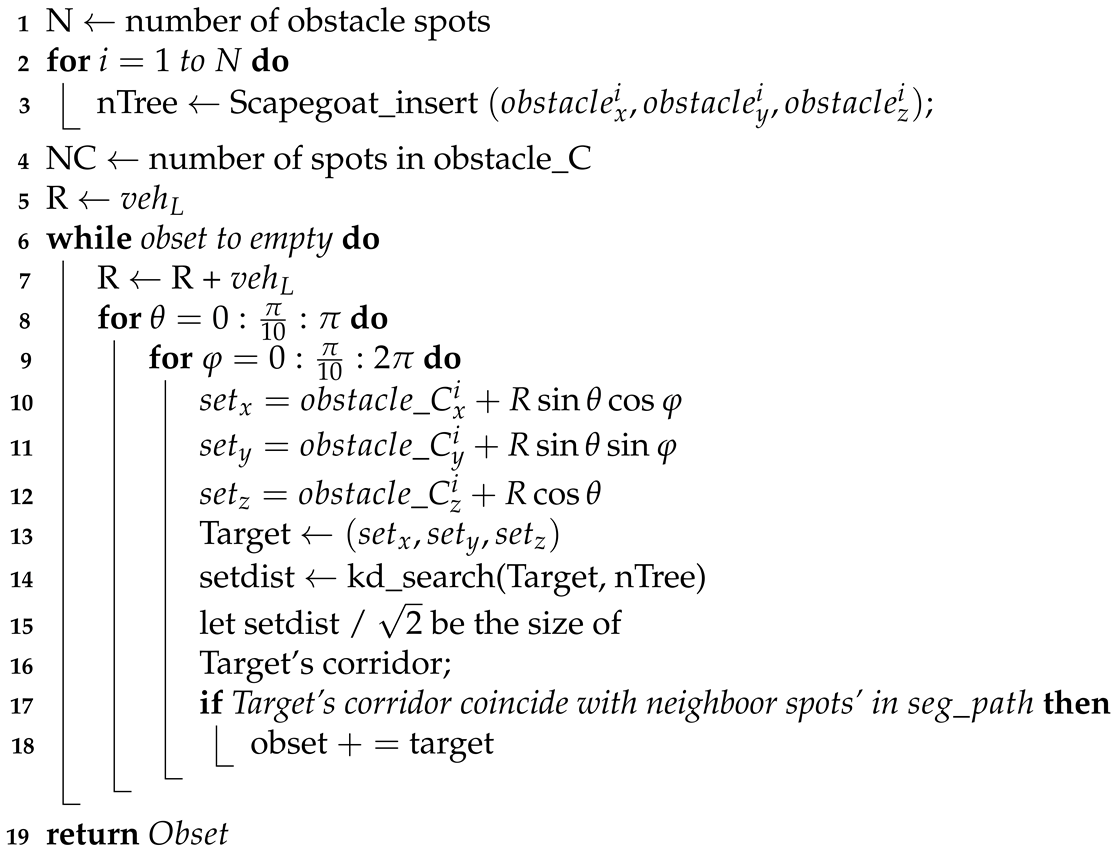
Recall our former assumption of unknown obstacles: we created irregularly shaped obstacles in random locations. The detailed strategy is shown in Algorithm 1.

To prevent collisions, we need to search for free spaces surrounding the obstacle. To replan the whole path to be as short as possible, the replanned path segment should be as close to the former path as possible. In other words, the newfound points should be as near as possible to obstacles but ensure no collisions at the same time. To store the information of obstacles, we use a scapegoat tree to insert them into $terTree$. We update the $treTree$ with the scapegoat tree, or simply reconstruct another KD tree $obTree$ with points on the obstacle’s surface.

Based on space-partitioning, the KD tree is a data structure that is able to organize points in k-dimensional space. Since the KD tree is balanced, inserting points into it may lead to very deep sorting. However, reconstruction is unnecessary and increases the time cost for the whole algorithm. We solve this problem using the scapegoat tree. The scapegoat tree uses reconstruction criterion $\alpha$ to ensure the balance of a tree. When a new point is inserted into a tree, trials are conducted to check if any sub-tree contains too many nodes in one side. Our approach to record unknown obstacles is demonstrated in Algorithm 2. We get a flat node from the sub-tree by orderly traversal.

Algorithm 1: Generate the randomly unknown obstacles.

Input: Origin Tree of terrain treTree

segment path:segpath;

number of spots in segpath: num;

length if vehcle:$ve{h}_L$

size of corridor for spots in segpath

Ouput: obstacles spots: obstacles;

center of obstacles: obstacle_C;

For obstacle $ob{s}_s$ in the path segment between $p_{m+i}$ and $p_{m+i+1}$, a circumscribed sphere $SP{H}_s^1$ with the farthest distance $r_s^1$ from $[ob{s}_s^1,ob{s}_s^2,...ob{s}_s^k]$ as the radius can be drawn out of $SP{H}_s^1$, which is free of obstacles. Let $SP{H}_s^2$ be the extension of $SP{H}_s^1$, whose radius is denoted as $r_s^2=ve{h}_L+r_s^1$. Spots on $SP{H}_s^2$ are the nearest spots to obstacles that can ensure safe flight for the HAUV. With the purpose of generating a smooth, safety trajectory, we tend to form corridors to record free space, which are used as space constraints (as shown in the next section). Here we focus on the approach to calculate specific size parameters of corridors. A trajectory can be generated only if all corridors coincide. With unknown environmental information recorded, let $D_{obs}^j$ be the shortest distance between obstacle $ob{s}_s$ and $SP{H}_s^2$. $D_{mi}$ is denoted as the minimum distance between $p_{m+i}(x_{m+i},y_{m+i},z_{m+i})$ and $ob{s}_s$. The side length $L_{mi}$ of each cube corridor is defined as follows:

$$L_{mi}=\sqrt{2}\ast D_{mi}$$

(10)

As illustrated in Figure 10, a sphere with a radius equal to $D_{mi}$ is circumscribed to mark free space.

Algorithm 2: Scapegoat_insert.

Input: spots to be inserted: obstacle;

The orgin tree: treTree;

control parameter: α

Ouput: newly constructed tree: treTree

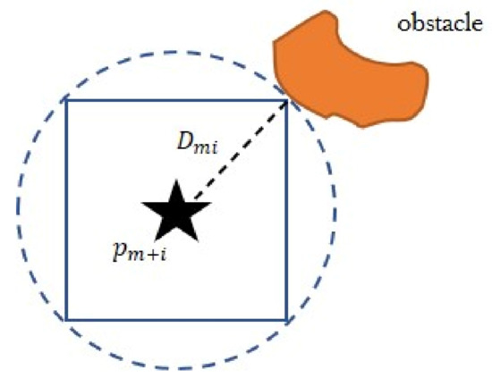
Figure 10. Generating the corridor size for target spots found on $SP{H}_s^2$. If the corridor intersects with the $p_{m+i}^{\prime }s$ and $p_{m+i+1}^{\prime }s$ corridor, then the spots will be recorded in the target spots set.

We use a square instead of a circle to record the free space, because it can easily set constraints at each axis out of $x,y,z$ in Cartesian coordinates, as is shown in Figure 11.

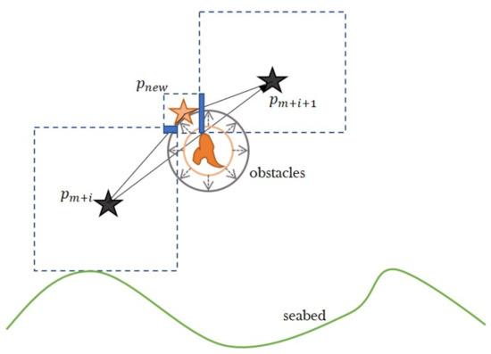
Figure 11. Two-dimensional corridors of $p_{new}$ and $p_{m+i}^{\prime }s$ and $p_{m+i+1}^{\prime }s$. In this condition, if the corridor of $p_{new}$ intersects with the $p_{m+i}^{\prime }s$ and $p_{m+i+1}^{\prime }s$ corridor, then the spots will be recorded as part of the target spots set.

Therefore, the trajectory between $p_{m+i}$ and $p_{m+i+1}$ exists only when:

$$\begin{array}{cc}\hfill & \frac{D_{obs}^j}{\sqrt{2}}+\frac{D_{mi}}{\sqrt{2}}\ge \left|x_{ob}-x_{m+i}\right|\hfill \\ \hfill & \frac{D_{obs}^j}{\sqrt{2}}+\frac{D_{mi}}{\sqrt{2}}\ge \left|y_{ob}-y_{m+i}\right|\hfill \\ \hfill & \frac{D_{obs}^j}{\sqrt{2}}+\frac{D_{mi}}{\sqrt{2}}\ge \left|z_{ob}-z_{m+i}\right|\hfill \\ \hfill & \frac{D_{obs}^j}{\sqrt{2}}+\frac{D_{mi+1}}{\sqrt{2}}\ge \left|x_{ob}-x_{m+i+1}\right|\hfill \\ \hfill & \frac{D_{obs}^j}{\sqrt{2}}+\frac{D_{mi+1}}{\sqrt{2}}\ge \left|y_{ob}-y_{m+i+1}\right|\hfill \\ \hfill & \frac{D_{obs}^j}{\sqrt{2}}+\frac{D_{mi+1}}{\sqrt{2}}\ge \left|z_{ob}-z_{m+i+1}\right|\hfill \end{array}$$

(11)

The points that satisfy the geometric constraints are recorded in expected points set $obset$. Given a large enough graph map, each obstacle $ob{s}_s$ should have at least one such set of points $obse{t}_s$. The method of searching available points on a collision-free sphere is demonstrated in Figure 12.

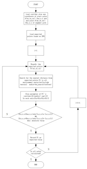
Figure 12. Algorithmic framework of obset (the set of collision-free spots on $SP{H}_s^{2,3,..}$) searching. With the coordinates and corridor sizes of spots in the original path segment, the program will run until spots expected on $SP{H}_s^{2,3..}$ are found. Let the expected spots be an obset.

If no expected points on $SP{H}_s^2$ are found, the radius R will be extended by step size r, and searching will keep going until at least one expected point is recorded. The flow chart of the whole obstacle avoidance method is shown in Figure 13a (sacpegoat tree) and Figure 13b (reconstructing trees).

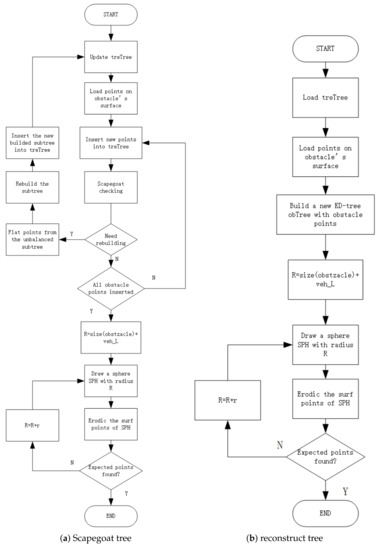
Figure 13. Flow Chart For obstacle avoidance, both the scapegoat tree and KD tree reconstruction methods are illustrated. In the scapegoat tree method, the obstacle spots are inserted into the original $treTree$, whereas the replanning method constructs a new KD tree from obstacle spots.

The inputs of the scapegoat tree are the coordinates of obstacle spots, the centers of the obstacles, the path segment, and the original $treTree$. After all obstacle spots are inserted into $treTree$, the radius of the collision-free sphere will be updated until expected spots are found. Obstet contains all the expected spots and is the output of this part of the program. Details are shown in Algorithm 3. On the other hand, the replanning method constructs a new KD tree from obstacle spots, as shown in Algorithm 4.

Algorithm 3: Use scapegoat tree to get collision-free spots around obstacles.

Input: Obstacle, Obstacle_C,

segpath; treTree;

Ouput: Clusters of collision free sets around obstacles: obset;

Algorithm 4: Reconstructing a KD tree for each obstacle.

Input: obstacle; obstacle_C

Ouput: obsets, KD tree constructed by obstacles: OBTree, treTree

With $obset$ determined, our best path is then updated as $\mathsf{\Phi }$$\left\{p_1,p_2,\dots obsets,\dots p_{n+1}\right\}$. The problem is then extended to a GTSP problem again: picking a sequence of spots within the $n+1$ group. All these groups of spots except $obset$ contain only one spot, while $obset$ contains all the available spots on the free sphere. After that, an updated best path $\mathsf{\Phi }$ becomes the input for the trajectory generation algorithm.

4. Trajectory Generation

With a sequence of target spots, our goal is to find a trajectory that holds the following properties: For each trip ${\mathsf{\Gamma }}_i$ between $p_i$ and $p_{i+1}$, the HAUV should work within its motion capabilities. The whole trajectory must be collision-free; the position, velocity, and acceleration at each spot $p_i$ are continuous.

Therefore, the function polynomial $f_t$ that denotes the position of the HAUV should be subject to such constraints. Furthermore, we use methods to minimize the snap of $f_t$ and minimize differential thrust to make the whole trip maximally efficient. Therefore, the problem is converted to a convex problem. using a Bernstein basis that conforms to the former constraints to represent piecewise trajectory, the output will be guaranteed to satisfy motion, safety, boundary, and continuity requirements.

4.1. Bézier Curve

We use a Bernstein polynomial basis to represent each trip between two target spots. The position of HUAV for each trip in each dimension out of $\left[x,y,z\right]$ can be written as:

$$f_j^{x,y,z}\left(t\right)=\sum _{i=0}^u{c}_i\left(\genfrac{}{}{0pt}{}{u}{i}\right)\ast t^i\ast {\left(1-t\right)}^{u-i}$$

(12)

Since variable t of Bernstein polynomials is defined on a fixed interval $\left[0,1\right]$, as in [37], we use scale s to scale the parameter time t to an arbitrarily allocated time for each segment. Then the whole trajectory that contains n piecewise trajectory with the degree of u can be generalized to Equation (13). In the following part of this section, we will briefly use F to represent the whole trajectory, and $f_j$ to describe the $j_{th}$ piecewise trajectory as well.

$$F^{x,y,z}\left(t\right)=\left\{\begin{array}{c}{s}_1{f}_0^{x,y,z}\left(\frac{t-T_0}{s_1}\right),t\in \left[T_0,T_1\right]\hfill \\ s_2{f}_1^{x,y,z}\left(\frac{t-T_1}{s_2}\right),t\in \left[T_1,T_2\right]\hfill \\ ⋮\hfill \\ s_n{f}_{x,y,z}^n\left(\frac{t-T_{n-1}}{s_n}\right),t\in \left[T_{n-1},T_n\right]\hfill \end{array}\right.$$

(13)

We set the time $T_j$ to demonstrate the time in which the HAUV is supposed to achieve the path segment, by assuming the HAUV travels with trapezoidal velocity, which will be introduced in the following section.

4.2. Constraint Settings

4.2.1. Motion Constraints

As we mentioned before, the trip ${\mathsf{\Gamma }}_i$ between $p_i$ and $p_{i+1}$ may not be in a single domain. Considering the specific environment between each pair of spots, the mode of travel for the HAUV between $p_i$ and $p_{i+1}$ can be divided into four types. Furthermore, the velocity and acceleration should be set pre-mission according to the modes: $underwater,aerial,transitioning\left(betweenwaterandair\right)$. Given the hodograph property of the Bézier curve—that the derivative $F^{\prime }$ of the trajectory function F still satisfies the constraints—the motion capabilities of the HAUV involving consideration of the control points $\left\{c_1^{\prime },c_2^{\prime },\dots ,c_n^{\prime }\right\}$ of $F_t^{\prime }$ are denoted as:

$$\begin{array}{c}\hfill c_i^{\left(n\right)}=n\ast (c_{i+1}^{(n-1)}-c_i^{(n-1)})\end{array}$$

(14)

As F illustrates the trajectory, velocity can be determined by $F_j^{\prime }$, and acceleration can be determined by $F_j^{″}$. Therefore, for each piece of trip the motion, constraints can be generalized to:

$$\begin{array}{cc}\hfill & |v_{max}^k|\ge n·(c_{k+1}-c_k)\hfill \\ \hfill & |a_{max}^k|\ge n·(n-1)·(c_{k+2}-2·c_{k+1}+p_k)\hfill \end{array}$$

(15)

The constraints of velocity and acceleration are taken into consideration in this way.

4.2.2. Safety Constraints

To guarantee the safety constraints, we use flight corridors to illustrate safe zones for the HAUV; in these corridors, it can move safely without collision. Since most of the obstructions in the underwater environment come from the terrain of the sea bed, by constructing a KD tree $treTree$ for all known terrain information $TE$, we can quickly figure out the shortest distances $dis{t}_i$ between the $p_i$ and the obstacles’ spots $m_i$∈$TE$. By setting a corridor whose width equals $dis{t}_i$, the safety of the trajectory is ensured. However, for some spots far away from obstacles or terrain barriers, such constraints may be too loose. In this case, let $d_i$ be the shortest distance between pi and its neighboring spot/spots. We define the smaller one as $dis{t}_i$ and $d_i$ as the width $W_i$ of the $i_{th}$ corridor.

4.2.3. Time Allocation

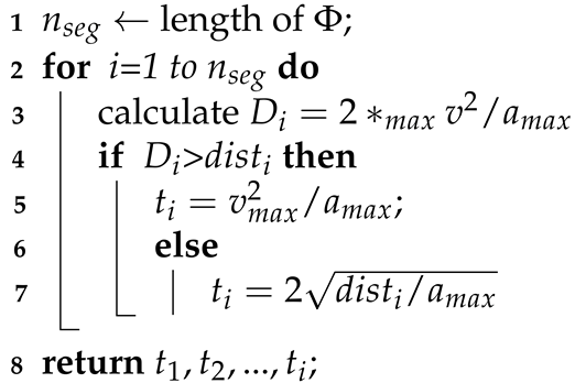
To allocate time, we assume HAUVs travel with trapezoidal velocity: HAUVs always move at maximal acceleration. To enable an HAUV to cover all the target spots, we allow the duration to be as flexible as possible, assuming the HAUV accelerates from 0 m/s at each spot. For each target spot $p_i$, we quickly search the widths of corridors by the former methods. Let $D_i=\frac{2v_{max}^2}{a_{max}}$ be a criterion that demonstrates the distance the HAUV covers when it moves at maximum velocity and acceleration. If $dis{t}_i\ge D_i$, the HAUV accelerates until maximum velocity and then slows down to 0 m/s at the destination. It cannot cover the whole lengths of most trips that way, so we assume that the HAUV moves at maximum velocity for a while and then slows down. Otherwise, the HAUV will not have enough time to accelerate to full velocity, so we assume it keeps moving at maximum acceleration. Therefore, reasonable corridors and time duration have been set for trajectory generation. Details are in Algorithm 5.

Algorithm 5: Arbitrary time duration t1, t2, ..., tn for HUAV to travel through spots.

Input: The sequence of spots Φ;

The maximum velocity, $v_{max}$, accelerate $a_{max}$;

The nearest distances between each spots and obstacles dist1, dist2, ..., distn;

Ouput: Time duration T1, T2, ..., Tn for each trip;

4.2.4. Continuous Constraint

During a real-time operation, the position, velocity, and acceleration at the spot $p_i$ must be continuous to make the curve consecutive:

$$\begin{array}{cc}\hfill & f_j\left(T_j\right)=f_{j+1}\left(T_j\right)\hfill \\ \hfill & f_j^{\left(1\right)}\left(T_j\right)=f_{j+1}^{\left(1\right)}\left(T_j\right)\hfill \\ \hfill & F_j^{\left(2\right)}\left(T_j\right)=F_{j+1}^{\left(2\right)}\left(T_j\right)\hfill \end{array}$$

(16)

With all the constraints mentioned above, we used the QP-solver in MATLAB to seek control points in each piece of the trajectory that minimized the snap of the trajectory function:

$$\begin{array}{c}\hfill \mathbf{minimize}:F_t^{\left(4\right)}\left(t\right)\end{array}$$

(17)

The output trajectory function is discussed in Section 5.1.2 and Section 5.2.2. The velocity and acceleration data are illustrated in Section 5.1.3.

5. Simulation Results

Through simulations, we evaluated the efficiency of the proposed algorithm and drew conclusions about motion control parameters: velocity and acceleration of the whole trip. All experiments were performed in MATLAB 2018a in Windows 10 on a computer with Intel i7-750U, 3.5 GHZ, and 8GB RAM. Based on fractional Brownian motion, we drew several 3-dimensional maps via a simple algorithm with a strictly geometrical interpretation.

The inputs for our algorithm were k groups of information spots in a map of size $x_{max}\ast y_{max}\ast h_{max}$. Spots in each group obey a Gaussian distribution. For each dimension out of x,y,z, the covariance $CO{V}_i$ for the $i_{th}$ group is denoted as $CO{V}_i=h_{max}/2\ast r$, where r means a random real number varies from 0 tp 1. The expectations $e_{x,y,z}^i$ are explained in Equation (18):

$$\begin{array}{cc}\hfill & e_x^i=x_{max}\ast rand(K,1)\hfill \\ \hfill & e_y^i=y_{max}\ast rand(K,1)\hfill \\ \hfill & e_z^i=h_{max}\ast rand(K,1)\hfill \end{array}$$

(18)

The number $num$ that describes the amount of spots that each group contains is also randomly defined as an integral number at given ranges: $num\in$$\left[1,2x_{max}\right]$.

Furthermore, we set a case that take the current fields into consideration. The current fields are created based on real-world data and have velocity in 3 dimensions. They may cost more or less energy cost of the HAUV mission, which refers to the direction and value of the currents surrounding the HAUV. An example of the current fields in our work is as Figure 14.

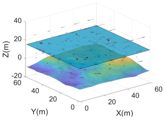
Figure 14. An example of current fields. The field are for underwater and aerial environments. We made the assumption that the surface of the water will remain flat during transitions of the vehicle from air to water, and vice versa.

5.1. Multi-Domain Coverage Planning in Static Environments

5.1.1. Path Searching

Firstly we clustered the random spots into groups via KMEANS solver. Then, the coordinate and set number of each spot were put into the GLNS algorithm. The coordinates of the center of each spot were the input of ACO.In our work, the parameters selected for ACO were as in Table 2.

Table 2. The parameters chosen for the ACO in this work.

$\mathit{The}\mathit{Parameters}$	$\mathit{Value}$
Number of ants	75
Volatilization of pheromone trail	0.2
Influence of pheromone	1
Influence of heuristic values	4
The constant Q	10
The max times of iterations	100
Heuristic function	1/D; where D is the weighted distance between two spots.

A comparison is illustrated in Figure 15. The output of GLNS is shorter than that of ACO.

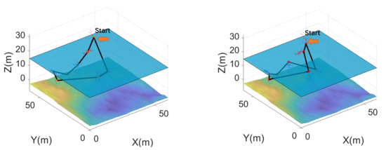
Figure 15. A comparison of the paths generated by ACO and GLNS. In this scenario, 189 spots were divided into eight groups. The HAUV began at one spot and went back to the starting spot when the mission was finished. With the conditions in the table above, the total length of the path found by ACO was 719.0682 within 1.037 s, whereas GLNS’s path was 528.578, found in 3.0140 s.

The total weighted distance of the path output by GLNS is much shorter than that of ACO, whereas ACO was faster. Furthermore, we present the weighted lengths of paths under five scenarios. The numbers of sets and information spots and lengths of GLNS and ACO outputs are in Table 3.

Table 3. The distances of GLNS and ACO paths. On average, the paths of ACO were $1.6587$ times the weighted lengths of those of GLNS.

$\mathit{Sets}$	$\mathit{Information}\mathit{Spots}$	$\mathit{GLNS}$	$\mathit{ACO}$
5	25	209.48	390.795
10	205	564.75966	909.442
15	426	640.2459	1076.1183
20	421	197.42732	199.3851
25	525	769.062302	1373.5974

5.1.2. Trajectory Generation

The output paths of GLNS and ACO were put into the trajectory generator. Through searching in KD tree $treTree$ built of terrain map $Map$, the length of the corridor was set. Then, trajectories were generated for the GLNS and ACO paths. Output examples are illustrated in Figure 16.

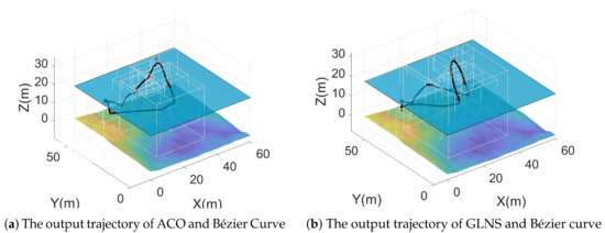
Figure 16. A comparison of the trajectories generated with the GLNS path and the ACO path using a Bézier curve. KD trees, corridors, and whole trajectories are illustrated. In this scenario, the weighted length of the ACO trajectory was 924.6468, and GLNS’s was 645.4758.

5.1.3. Velocity and Acceleration

The HUAV is commanded to follow the waypoints provided by its path planning system. The dynamic states of the vehicle achieving this trajectory are shown in FigureFigure 17. In this case, the HAUV performed differently in multiple environments. The maximum velocity in the air was 9.5 m/s, and it was 2.74 m/s underwater; and the maximum acceleration in the air was $3{\mathrm{m}}^2/\mathrm{s}$, and it was $0.78{\mathrm{m}}^2/\mathrm{s}$ underwater. All the outputs of the motion parameters conform to the HAUV’s motion capability. The trajectory passed through all the target spots given by the GLNS solver safely. Figure 17shows the corresponding resultant velocity and acceleration of the HAUV as it tracked through the trajectory. It can be clearly seen that the HAUV was in a different mode when operating in dynamic environments: moving in the air or moving underwater. Therefore, the values of velocity and acceleration would be helpful for HAUV control.

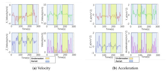
Figure 17. The velocity and acceleration of one HAUV on a typical mission. The underwater and aerial modes can be distinguished from this figure: aerial velocity and acceleration constraints are looser than underwater condition ones.

5.2. Multi-Domain Informative Path Planning for Unknown Obstacles and Current Fields

The inputs of the path replanning solver are subpaths of the original path and unknown obstacles. Within the succession of spots, obstacles may appear in arbitrary locations between pairs of neighboring spots with certain probabilities.

We present two methods to replan the path: reconstructing a KD tree for unknown obstacles or insert unknown obstacles into the $treTree$ through the scapegoat tree. The outputs of these two methods are all the same, but the duration can vary. A detailed comparison is shown in Table 4.

Table 4. This table shows a comparison between the scapegoat tree and KD tree reconstruction replanning methods. $Map$ refers to the size of the original terrain map; R refers to the radius in which expected points are located; $obs$ refers to the number of points this obstacle contains; $sets$ refers to the number of potential expected points; $T_{sp}$ refers to the time cost of scapegoat; $T_{re}$ refers to the time cost of reconstruction $treTree$.

$\mathit{Map}$	$\mathit{R}(/{\mathit{veh}}_{\mathit{L}})$	$\mathit{obs}$	$\mathit{Sets}$	${\mathit{T}}_{\mathit{sp}}(/\mathit{s})$	${\mathit{T}}_{\mathit{re}}(/\mathit{s})$
100*100	100	121	121	0.6950	0.6240
20*20	100	441	121	0.2030	0.2710
20*20	10	441	121	0.4490	0.2840
20*20	10	121	411	0.2070	0.1900
20*20	100	36	121	0.940	0.1080

5.2.1. Replan Methods

The time complexity of KD tree construction is $O\left(lo{g}^{2}n\right)$—the insert has $O\left(lo{g}^{2}n\right)$ complexity; searching in k-dimensions is $O(n^{1-\frac{1}{k}}+1)$-complex, and using a scapegoat tree to insert can be generalized to $O\left(logn\right)$. Paths replanned by the scapegoat tree and the reconstructed tree were the same most of the time. For each round of $obset$ searching, the performances of the two methods were different: when inserting/reconstructing many discrete target points, the scapegoat method performed better; when coping with dense, small numbers of points, the reconstructed tree method performed better. A possible reason is: consider the additional time taken to reconstruct a whole tree compared to a few insertions; but traversal through and insertion into a sub-tree is time consuming, so many points could reverse the situation. The geometric density of obstacle points can lead to unbalancing of the KD tree. When inserted into a tree, they are high-probability in the same sub-tree. Similarly, when there are a small number of discrete obstacles on a relatively large-scale map, few reconstruction processes for sub-tree are required. Another probable reason for our observations is that, since a map is much larger than any obstacle, the time taken to insert an obstacle into the map is longer than that taken to reconstruct a new tree for obstacle information.

In conclusion, the scapegoat tree should be used for small areas with discretely located obstacles having simple geometrical features. In large maps with dense obstacles, reconstructing a KD tree would improve performance.

5.2.2. An Example of a Replanned Path and Its Trajectory

Compared to the former path, the new path should avoid obstacles. Trajectory generation methods also provide smooth, safe outputs. Figure 18 gives an example of a replanning path. The replanned path segment is marked in red:

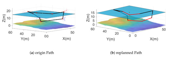
Figure 18. A comparison of an entire original path and a replanned path. Two obstacles appeared within the duration. The weighted length of the original path was 505.301308. The partly replanned path is red.

The regenerated whole trajectory is shown in Figure 19. The number of spots for the obstacle set was 49; each iteration of R 100 spots on the collision-free sphere was traversed:

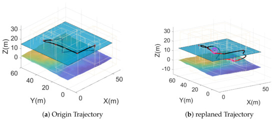
Figure 19. A comparison of a whole original path and a replanned path. Two obstacles appeared within the duration. The weighted length of the trajectory was 863.7285. The partly replanned path is marked in red. Collision-free spots on the free sphere around obstacles are illustrated as free obsets. The number of spots in the obstacle set was 49. Each iteration of R 100 spots on the collision-free sphere was traversed.

A detailed look at the replanned path and the trajectory of a path segment are shown in Figure 20. The number of spots in the obstacle set was 49. Each iteration of R 100 spots on the collision-free sphere was traversed.

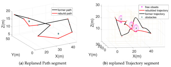
Figure 20. Details of the replanned trajectory and path. Collision-free spots on the free sphere around obstacles are illustrated as free obsets. The number of spots in the obstacle set was 49. Each iteration of R 100 spots on the collision-free sphere was traversed.

5.2.3. Path Replanning and Trajectory Generation in Current Fields

As in the previous cases, we reconstructed a path, only, one that passed through current fields, which can have a significant influence on an HAUV. In this case we set the influence indicator $\eta =0.3$. In Figure 21, the replanned path is marked in red. A comparison between paths in environments with and without current is demonstrated in Table 5. The overall costs of the original path and the path with current have no big gaps. That may be because currents can have both positive and negative influences on the energy costs in a trip, depending on their directions. These two kinds of influence may offset each other.

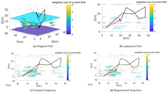
Figure 21. The replanned path and trajectory in current fields. The weighted costs of recorded strong currents fields are illustrated. The original path and trajectory passed through or quite near to (distance < vehicle length) strong current fields, which would be unsafe and involves a high energy cost. The replanned path and trajectory avoided such areas. The weighted cost of avoiding the current was 770.2315, and to not avoid it was 810.1669 in this case.

Table 5. The weighted distance costs of planned paths with and without current fields. There are small differences between the outputs of these two scenarios. A possible reason is the positive and negative influences of current fields offsetting each other.

$\mathit{Sets}$	$\mathit{Information}\mathit{Spots}$	$\mathit{Origin}\mathit{Path}$	$\mathit{Path}\mathit{with}\mathit{Currents}$
5	25	209.48	212.3
10	205	564.75966	541.3
15	426	640.2459	650.2432
20	421	197.42732	205.4523
25	525	769.062302	777.8012

5.3. Monte Carlo Simulations

Under static conditions, we performed Monte Carlo experiments with 100 runs in five scenarios. The solutions drawn by GLNS are much better than those drawn by ACO. The number of sets varied from 5 to 25, average 15; the number of information spots varied from 20 to 587, average 336.

With the unknown obstacles, we performed Monte Carlo experiments with 100 runs in five scenarios. The number of sets varied from 5 to 25, average 14.7100; the number of obstacle sets on each path averaged 5.8. The average radius of the collision-free spheres around obstacles when free spots were found was $R=2.3ve{h}_L$. Over 90% percent of runs could figure out the free spots within the first iteration of the collision-free sphere. Each iteration of R 100 spots on the collision-free sphere was traversed. The number of obstacle spots in each set varied from 49 to 100. The results of static and unknown obstacle simulations are both illustrated in Figure 22. One-hundred runs with a current field are illustrated in Figure 23. We considered a scenario in which the currents were weak. The average velocity of currents in the air was 0.97 m/s, and underwater, 0.26 m/s.

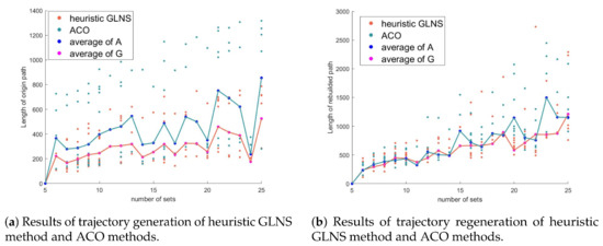
Figure 22. Outputs of 100 runs are scattered, and the average values are illustrated as lines. Generally speaking, heuristic $GLNS+KMEANS+KDtree$ performed better than a common TSP solver.

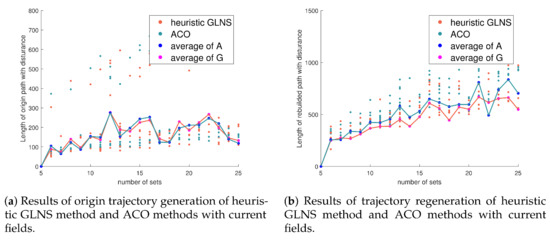
Figure 23. Outputs of 100 runs are scattered, and the average values are illustrated as lines. Generally speaking, with current fields, heuristic $GLNS+KMEANS+KDtree$ performed better than a common TSP solver. The total weighted cost changeed slightly with currents. The average velocity of current was 0.26 m/s underwater, and it was 0.97 m/s in the air.

The original trajectory drawn by heuristic $GLNS+KMEANS+KDtree$ was better than ACO 88 times out of 100 runs. The average weighted cost of the former was 279.4952, and that of the latter was 432.5474. However, when it comes to the regeneration, heuristic $GLNS+KMEANS+KDtree$ performed better 72 times out of 100 runs, especially when the number of sets was enormous. The average weighted cost of the heuristic GLNS’s regenerated trajectory was 585.8950, and that of ACO’s trajectory was 674.8518.

6. Conclusions

This paper proposed a general framework for multidomain environmental monitoring, which is especially beneficial for the novel multidomain vehicles. The presented heuristic GLNS with KMEANS methods can plan an efficient path that satisfies the information selecting requirements. The approach combines the Bézier curve and the KD-tree to generate an optimal trajectory in a multidomain environment while conforming to the vehicle’s motion capabilities. We also considered scenarios that contain random obstacles and current fields. The problem is generalized to a fixed-radius near neighbors problem, and the path is rebuilt based on a KD-tree or scapegoat tree.

Our approach was evaluated through numerical MATLAB simulations using real-world terrains and current data. Our method adopts the k-means clustering process to discrete informative spots. The path planning method performed better than common TSP solvers, such as the ACO algorithm. Two path replanning approaches were presented, and a comparison of their appropriate usage conditions was listed. Furthermore, field experiments will be performed once our HAUV is equipped with visual devices.

In the future, the theoretical work will focus on more complex dynamic environments. We also intend to challenge our HAUV with multi-robot missions. Cooperation tasks with other vehicles, such as UAVs, UUVs, and UGVs, will be the focus.

References

- Lu, D.; Xiong, C.; Zeng, Z.; Lian, L. Adaptive dynamic surface control for a hybrid aerial underwater vehicle with parametric dynamics and uncertainties. IEEE J. Ocean. Eng. 2019, 45, 740–758. [Google Scholar] [CrossRef]
- Weisler, W.; Stewart, W.; Anderson, M.B.; Peters, K.J.; Gopalarathnam, A.; Bryant, M. Testing and characterization of a fixed wing cross-domain unmanned vehicle operating in aerial and underwater environments. IEEE J. Ocean. Eng. 2017, 43, 969–982. [Google Scholar] [CrossRef]
- Stewart, W.; Weisler, W.; MacLeod, M.; Powers, T.; Defreitas, A.; Gritter, R.; Anderson, M.; Peters, K.; Gopalarathnam, A.; Bryant, M. Design and demonstration of a seabird-inspired fixed-wing hybrid UAV-UUV system. Bioinspir. Biomim. 2018, 13, 56013. [Google Scholar] [CrossRef] [PubMed]
- Drews, P.L.; Neto, A.A.; Campos, M.F. Hybrid unmanned aerial underwater vehicle: Modeling and simulation. In Proceedings of the 2014 IEEE/RSJ International Conference on Intelligent Robots and Systems, Chicago, IL, USA, 14–18 September 2014; pp. 4637–4642. [Google Scholar]
- da Rosa, R.T.; Evald, P.J.; Drews, P.L.; Neto, A.A.; Horn, A.C.; Azzolin, R.Z.; Botelho, S.S. A comparative study on sigma-point kalman filters for trajectory estimation of hybrid aerial-aquatic vehicles. In Proceedings of the 2018 IEEE/RSJ International Conference on Intelligent Robots and Systems (IROS), Madrid, Spain, 1–5 October 2018; pp. 7460–7465. [Google Scholar]
- Maia, M.M.; Soni, P.; Diez, F.J. Demonstration of an aerial and submersible vehicle capable of flight and underwater navigation with seamless air-water transition. arXiv 2015, arXiv:1507.01932. [Google Scholar]
- Alzu’bi, H.; Mansour, I.; Rawashdeh, O. Loon copter: Implementation of a hybrid unmanned aquatic–aerial quadcopter with active buoyancy control. J. Field Robot. 2018, 35, 764–778. [Google Scholar] [CrossRef]
- Lu, D.; Xiong, C.; Zhou, H.; Lyu, C.; Hu, R.; Yu, C.; Zeng, Z.; Lian, L. Design, fabrication, and characterization of a multimodal hybrid aerial underwater vehicle. Ocean Eng. 2021, 219, 108324. [Google Scholar] [CrossRef]
- Choset, H. Coverage for robotics—A survey of recent results. Ann. Math. Artif. intell. 2001, 31, 113–126. [Google Scholar] [CrossRef]
- Galceran, E.; Carreras, M. A survey on coverage path planning for robotics. Rob. Auton. Syst. 2013, 61, 1258–1276. [Google Scholar] [CrossRef] [Green Version]
- Choset, H.; Pignon, P. Coverage path planning: The boustrophedon cellular decomposition. In Field and Service Robotics; Springer: Berlin/Heidelberg, Germany, 1998; pp. 203–209. [Google Scholar]
- Choset, H.; Acar, E.; Rizzi, A.A.; Luntz, J. Exact cellular decompositions in terms of critical points of morse functions. In Proceedings of the 2000 ICRA. Millennium Conference. IEEE International Conference on Robotics and Automation, Symposia Proceedings (Cat. No.00CH37065). San Francisco, CA, USA, 24–28 April 2000; Volume 3, pp. 2270–2277. [Google Scholar]
- Choset, H.M.; Lynch, K.M.; Hutchinson, S.; Kantor, G.; Burgard, W.; Kavraki, L.; Thrun, S.; Arkin, R.C. Principles of Robot Motion: Theory, Algorithms, and Implementation; MIT Press: Cambridge, MA, USA, 2005. [Google Scholar]
- Lewis, J.S.; Edwards, W.; Benson, K.; Rekleitis, I.; O’Kane, J.M. Semi-boustrophedon coverage with a dubins vehicle. In Proceedings of the 2017 IEEE/RSJ International Conference on Intelligent Robots and Systems (IROS), Vancouver, BC, Canada, 24–28 September 2017; pp. 5630–5637. [Google Scholar]
- Vandermeulen, I.; Groß, R.; Kolling, A. Turn-minimizing multirobot coverage. In Proceedings of the 2019 International Conference on Robotics and Automation (ICRA), Montreal, BC, Canada, 20–24 May 2019; pp. 1014–1020. [Google Scholar]
- Yu, K.; O’Kane, J.M.; Tokekar, P. Coverage of an environment using energy-constrained unmanned aerial vehicles. In Proceedings of the 2019 International Conference on Robotics and Automation (ICRA), Montreal, BC, Canada, 20–24 May 2019; pp. 3259–3265. [Google Scholar]
- Yu, K.; Budhiraja, A.K.; Buebel, S.; Tokekar, P. Algorithms and experiments on routing of unmanned aerial vehicles with mobile recharging stations. J. Field Robot. 2019, 36, 602–616. [Google Scholar] [CrossRef]
- Xiong, C.; Chen, D.; Lu, D.; Zeng, Z.; Lian, L. Path planning of multiple autonomous marine vehicles for adaptive sampling using Voronoi-based ant colony optimization. Rob. Auton. Syst. 2019, 115, 90–103. [Google Scholar] [CrossRef]
- Xiong, C.; Lu, D.; Zeng, Z.; Lian, L.; Yu, C. Path planning of multiple unmanned marine vehicles for adaptive ocean sampling using elite group-based evolutionary algorithms. J. Intell. Robot. Syst. 2020, 99, 875–889. [Google Scholar] [CrossRef]
- Xiong, C.; Zhou, H.; Lu, D.; Zeng, Z.; Lian, L.; Yu, C. Rapidly-Exploring Adaptive Sampling Tree*: A Sample-Based Path-Planning Algorithm for Unmanned Marine Vehicles Information Gathering in Variable Ocean Environments. Sensors 2020, 20, 2515. [Google Scholar] [CrossRef]
- Zeng, Z.; Lian, L.; Sammut, K.; He, F.; Tang, Y.; Lammas, A. A survey on path planning for persistent autonomy of autonomous underwater vehicles. Ocean Eng. 2015, 110, 303–313. [Google Scholar] [CrossRef]
- Zeng, Z.; Sammut, K.; Lian, L.; He, F.; Lammas, A.; Tang, Y. A comparison of optimization techniques for AUV path planning in environments with ocean currents. Rob. Auton. Syst. 2016, 82, 61–72. [Google Scholar] [CrossRef]
- Cao, J.; Cao, J.; Zeng, Z.; Yao, B.; Lian, L. Toward optimal rendezvous of multiple underwater gliders: 3D path planning with combined sawtooth and spiral motion. J. Intell. Robot. Syst. 2017, 85, 189–206. [Google Scholar] [CrossRef]
- Zeng, Z.; Sammut, K.; Lian, L.; Lammas, A.; He, F.; Tang, Y. Rendezvous path planning for multiple autonomous marine vehicles. IEEE J. Ocean. Eng. 2017, 43, 640–664. [Google Scholar] [CrossRef]
- Song, R.; Liu, Y.; Bucknall, R. A multi-layered fast marching method for unmanned surface vehicle path planning in a time-variant maritime environment. Ocean Eng. 2017, 129, 301–317. [Google Scholar] [CrossRef]
- Liu, Y.; Liu, W.; Song, R.; Bucknall, R. Predictive navigation of unmanned surface vehicles in a dynamic maritime environment when using the fast marching method. Int. J. Adapt. Control Signal Process. 2017, 31, 464–488. [Google Scholar] [CrossRef]
- Liu, Y.; Bucknall, R. Path planning algorithm for unmanned surface vehicle formations in a practical maritime environment. Ocean Eng. 2015, 97, 126–144. [Google Scholar] [CrossRef]
- Hollinger, G.A.; Mitra, U.; Sukhatme, G.S. Active and adaptive dive planning for dense bathymetric mapping. In Experimental Robotics; Springer: Berlin/Heidelberg, Germany, 2013; pp. 803–817. [Google Scholar]
- Hollinger, G.A.; Englot, B.; Hover, F.S.; Mitra, U.; Sukhatme, G.S. Active planning for underwater inspection and the benefit of adaptivity. Int. J. Rob. Res. 2013, 32, 3–18. [Google Scholar] [CrossRef]
- Cao, C.; Zhang, J.; Travers, M.; Choset, H. Hierarchical coverage path planning in complex 3d environments. In Proceedings of the 2020 IEEE International Conference on Robotics and Automation (ICRA), Paris, France, 31 May–31 August 2020; pp. 3206–3212. [Google Scholar]
- Jing, W.; Deng, D.; Xiao, Z.; Liu, Y.; Shimada, K. Coverage path planning using path primitive sampling and primitive coverage graph for visual inspection. In Proceedings of the 2019 IEEE/RSJ International Conference on Intelligent Robots and Systems (IROS), Macau, China, 3–8 November 2019; pp. 1472–1479. [Google Scholar]
- Vidal, E.; Palomeras, N.; Istenič, K.; Gracias, N.; Carreras, M. Multisensor online 3D view planning for autonomous underwater exploration. J. Field Robot 2020, 37, 1123–1147. [Google Scholar] [CrossRef]
- Zacchini, L.; Ridolfi, A.; Allotta, B. Receding-horizon sampling-based sensor-driven coverage planning strategy for AUV seabed inspections. In Proceedings of the 2020 IEEE/OES Autonomous Underwater Vehicles Symposium (AUV), St. Johns, NL, Canada, 30 September–2 October 2020; pp. 1–6. [Google Scholar]
- Paull, L.; Saeedi, S.; Seto, M.; Li, H. Sensor-driven online coverage planning for autonomous underwater vehicles. IEEE ASME Trans. Mechatron. 2012, 18, 1827–1838. [Google Scholar] [CrossRef]
- Mellinger, D.; Kumar, V. Minimum snap trajectory generation and control for quadrotors. In Proceedings of the 2011 IEEE International Conference on Robotics and Automation, Shanghai, China, 9–13 May 2011; pp. 2520–2525. [Google Scholar]
- Chen, J.; Liu, T.; Shen, S. Online generation of collision-free trajectories for quadrotor flight in unknown cluttered environments. In Proceedings of the 2016 IEEE International Conference on Robotics and Automation (ICRA), Stockholm, Sweden, 16–21 May 2016; pp. 1476–1483. [Google Scholar]
- Gao, F.; Wu, W.; Lin, Y.; Shen, S. Online safe trajectory generation for quadrotors using fast marching method and bernstein basis polynomial. In Proceedings of the 2018 IEEE International Conference on Robotics and Automation (ICRA), Brisbane, Australia, 21–25 May 2018; pp. 344–351. [Google Scholar]
- Hitz, G.; Galceran, E.; Garneau, M.È.; Pomerleau, F.; Siegwart, R. Adaptive continuous-space informative path planning for online environmental monitoring. J. Field Robot 2017, 34, 1427–1449. [Google Scholar] [CrossRef]
- Shkurti, F.; Xu, A.; Meghjani, M.; Higuera, J.C.G.; Girdhar, Y.; Giguere, P.; Dey, B.B.; Li, J.; Kalmbach, A.; Prahacs, C.; et al. Multi-domain monitoring of marine environments using a heterogeneous robot team. In Proceedings of the 2012 IEEE/RSJ International Conference on Intelligent Robots and Systems, Vilamoura-Algarve, Portugal, 7–12 October 2012; pp. 1747–1753. [Google Scholar]
- Drews, P.L.; Neto, A.A.; Campos, M.F. A survey on aerial submersible vehicles. IEEE Oceans 2009, 9, 4244-2523. [Google Scholar]
- Fix, E.; Hodges, J.L. Discriminatory analysis. Nonparametric discrimination: Consistency properties. Int. Stat. Rev. 1989, 57, 238–247. [Google Scholar] [CrossRef]
- Zhang, H.; Berg, A.C.; Maire, M.; Malik, J. SVM-KNN: Discriminative nearest neighbor classification for visual category recognition. In Proceedings of the 2006 IEEE Computer Society Conference on Computer Vision and Pattern Recognition (CVPR’06), New York, NY, USA, 17–22 June 2006; pp. 2126–2136. [Google Scholar]
- Han, E.H.S.; Karypis, G.; Kumar, V. Text categorization using weight adjusted k-nearest neighbor classification. In Pacific-asia Conference on Knowledge Discovery and Data Mining; Springer: Berlin/Heidelberg, Germany, 2001; pp. 53–65. [Google Scholar]
- Stanfill, C.; Waltz, D. Toward memory-based reasoning. Commun. ACM 1986, 29, 1213–1228. [Google Scholar] [CrossRef]
- Friedman, J.H.; Bentley, J.L.; Finkel, R.A. An algorithm for finding best matches in logarithmic expected time. ACM Trans. Math. Softw. (TOMS) 1977, 3, 209–226. [Google Scholar] [CrossRef]
- Silpa-Anan, C.; Hartley, R. Optimised KD-trees for fast image descriptor matching. In Proceedings of the 2008 IEEE Conference on Computer Vision and Pattern Recognition, Anchorage, AK, USA, 23–28 June 2008; pp. 1–8. [Google Scholar]
- Muja, M.; Lowe, D.G. Fast approximate nearest neighbors with automatic algorithm configuration. VISAPP 2009, 2, 331–340. [Google Scholar]
- Indyk, P.; Motwani, R. Approximate nearest neighbors: Towards removing the curse of dimensionality. In Proceedings of the Thirtieth Annual ACM Symposium on Theory of Computing, Dallas, TX, USA, 24–26 May 1998; pp. 604–613. [Google Scholar]
- Wang, J.; Wang, J.; Zeng, G.; Tu, Z.; Gan, R.; Li, S. Scalable k-nn graph construction for visual descriptors. In Proceedings of the 2012 IEEE Conference on Computer Vision and Pattern Recognition, Providence, RI, USA, 16–21 June 2012; pp. 1106–1113. [Google Scholar]
- Demir, E.; Bektaş, T.; Laporte, G. An adaptive large neighborhood search heuristic for the pollution-routing problem. Eur. J. Oper. Res. 2012, 223, 346–359. [Google Scholar] [CrossRef]
- Smith, S.L.; Imeson, F. GLNS: An effective large neighborhood search heuristic for the generalized traveling salesman problem. Comput. Oper. Res. 2017, 87, 1–19. [Google Scholar] [CrossRef]
Publisher’s Note: MDPI stays neutral with regard to jurisdictional claims in published maps and institutional affiliations. |
© 2021 by the authors. Licensee MDPI, Basel, Switzerland. This article is an open access article distributed under the terms and conditions of the Creative Commons Attribution (CC BY) license (https://creativecommons.org/licenses/by/4.0/).