Target Search Algorithm for AUV Based on Real-Time Perception Maps in Unknown Environment

Abstract

For the problem of AUV target searches in unknown underwater environments, a target search algorithm for AUVs based on a real-time perception map is proposed. Real-time perception maps, including target existence probability maps, uncertainty maps, and pheromone maps and their updating rules, are established. Attraction source maps and search status maps based on the environmental information detected by the AUV are established. The maps are used for the AUV to search for corner areas that are unknown to a high degree and areas with low coverage around the current location. At the same time, a release mechanism for attraction and revisiting pheromones is established by combining a neural excitation network algorithm to make the gradient spread in the pheromone grid map. By setting up a search revenue function based on real-time perception maps, an AUV search decision-making method is established. When the AUV finds a suspected target, the AUV approaches the suspected target. The path planning of the AUV is carried out through an improved artificial potential field method. The short-distance confirmation of the target and obstacle avoidance in the search process are realized. The simulation results show that the algorithm has high search efficiency. Additionally, when the target exists in a corner area, the probability of the AUV to quickly search for the target is fast and feasible.

1. Introduction

With the development of modern technology, human beings are increasingly dependent on marine resources. In recent years, due to the fact that autonomous underwater vehicles (AUVs) have good concealment, flexibility in underwater movement, economic applicability, and other technical characteristics of high-tech means, they have received extensive attention both in the military and civilian fields. Regarding the structure of the AUV system, due to the high communication requirements and low fault tolerance of the centralized multi-AUV coordination strategy, it has been gradually replaced by the distributed multi-AUV autonomous coordination strategy [1,2,3]. At present, the more commonly used research ideas are mainly divided into two types: top to bottom and bottom to top [4].

For the problem of target searches in an unknown environment, more extensive research has been carried out on land and in the sea and air [5]. Based on the theory of search, the traditional method designs the search route of the task area in advance from the perspective of maximizing the probability of target discovery. However, since the search environment of the actual task is unknown and cannot be planned offline in advance, the real-time target search algorithm has been studied in depth.

The authors of [6] proposed a full coverage search algorithm. The algorithm carries out a detailed search for obstacles or the vicinity of the searched area as far as possible without violating the full coverage search to prevent missing targets. However, when the width of the robot’s coverage area is greater than one-half of the path between obstacles, multiple repeated searches will occur. This increases the search time and reduces the efficiency of the search. The authors of [7] aimed at searching for underwater moving targets in Markov process, and proposed a heuristic search algorithm for underwater moving targets based on Markov process. However, this algorithm cannot solve the search problem of unknown target location and state. The authors of [8] introduced a flag bit, and established an environmental probability model based on a double probability matrix. Additionally, combined with the improved coevolutionary genetic algorithm, the optimal collaborative path is continuously generated online. This improves the accuracy of the UAV system’s perception of the environment and improves the target search efficiency of the entire mission. However, this algorithm requires certain initial environmental information and cannot be used in completely unknown underwater area search tasks. The authors of [9] considered the detection efficiency of sensors and the probability of false alarms, and proposed a collaborative search method driven by a revisit mechanism. It can reduce the probability of target omission and misjudgment. The authors of [10] proposed a multi-UAV collaborative target search method with a pheromone return visit mechanism. The algorithm can improve the UAV’s ability to search and capture targets, the ability to make return visits to areas with high uncertainty, and the efficiency of multi-UAV collaborative searches. However, this method does not consider searches of corner areas. Moreover, the update mechanism of the target existence probability and the release mechanism of pheromones are not fully applicable to the AUV target search problem. In addition, the distance between the surrounding grid of the pheromone release grid and the current grid is not considered when the pheromone gradient diffusion is considered. The authors of [11] proposed a behavior-based robot cluster model for effective search and rescue operations in unknown environments. The authors of [12] proposed a multi-robot search strategy based on a segmentation strategy. In order to improve the search efficiency of this algorithm, each robot needs to go to different areas of uniform size. First, the algorithm of the segmentation strategy is adopted, and then the boundary-based algorithm is used to detect the segmented area. The authors of [13] gave the model and approximate mathematical representation of the multi-object search problem in swarm robots, and drew the lower bound of the expected number of iterations on this basis. A new search strategy based on a probability finite state set was also proposed. The authors of [14] applied UAV swarm coordination technology to target searches. Based on the swarm and swarm energy, it provides robust formation control and dynamic environment information sharing, and uses a differential evolution algorithm to adapt its coordination logic to tasks. The authors of [15] aimed at the dynamic search process in unknown maps without any prior information. Raster map methods such as probability maps and pheromone maps constructed based on Bayes theory have been proposed and widely used. The authors of [16] propose an evolutionary algorithm that uses biogeography-inspired operators to efficiently evolve a population of candidate solutions to the optimal or near-optimal solution within an acceptable time. The authors of [17] proposed an algorithm based on target clustering and path optimization was proposed to reduce reactive consumption and obtain more revenue, which is conducive to a more thorough search of the target areas.

Combining the established real-time perception maps, including target existence probability maps, uncertainty maps, pheromone maps, and their update rules, an attraction source map is set up to make it easier for AUVs to search for corner targets. An AUV is guided to search the unsearched area based on the searched area map under the condition of low search coverage, so as to reduce the uncertainty of the search area more efficiently. Especially when the target exists in the corner of the area, the traditional search method may not find the target for a long time or at all. This study increases the feasibility and speed of searching corner areas by introducing the attraction source, which is more conducive to the search for the target in corner areas. Taking the characteristics of underwater AUV searches into consideration, a pheromone release mechanism and update formula that conform to the actual situation of underwater searches are designed. The AUV can revisit specific areas in the later stages of the search mission to prevent missing targets due to sonar sensing efficiency issues. The search revenue function is set based on the real-time perception map to make the optimal search decision. Since the AUV uses its own optical camera to determine the target at a short distance, the kinematics model of the AUV is considered. Combined with the corner constraint of the AUV, the artificial potential field method is improved to plan the path of the AUV. This method makes the AUV reach the search decision point or the suspected target point with a shorter path, which can reduce the fuel consumption during the search process and avoid the possibility of AUV collision.

2. Problem Description

In an unknown underwater search environment, an AUV equipped with sensors is used to search for N stationary targets in the target area $\Omega$. Since the AUV is not aware of the target location distribution and the obstacle distribution in the target area, the AUV needs to acquire and analyze the surrounding area’s information according to the mounted sensors. Combining the acquired information, the optimal search decision is made in real time according to the search algorithm. If a target is found within the detection range of the AUV’s sensor, it will determine the location of the suspected target based on the detection information. When the AUV approaches the suspected target at close range, it can confirm the target at close range through the mounted sensor.

2.1. AUV Movement Model

The kinematic model of the AUV is introduced in [18], so the search path planned by the algorithm proposed in this paper is more consistent with the actual situation in the AUV search process.

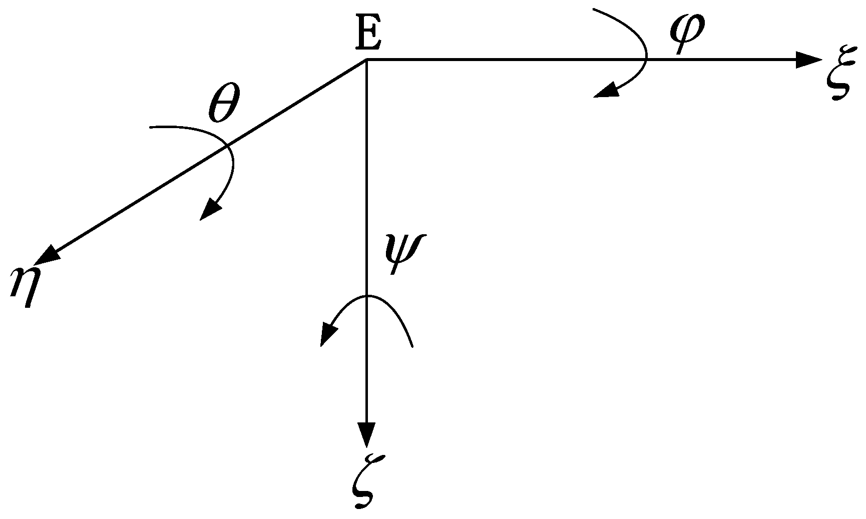
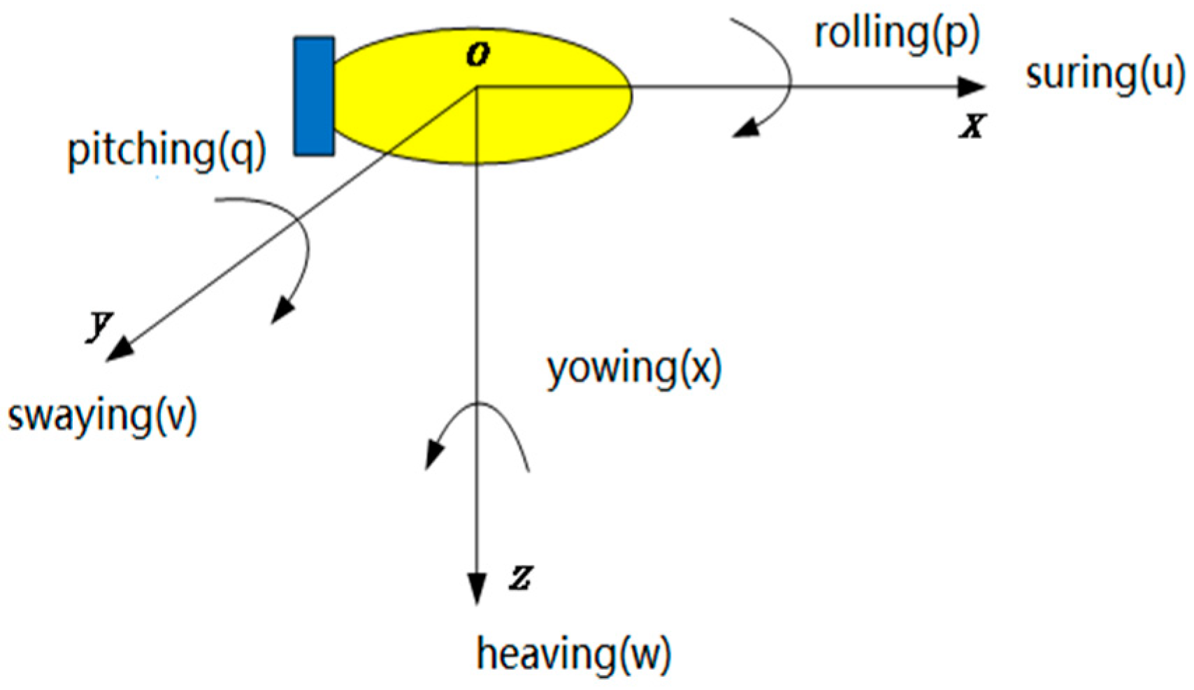
The inertial coordinate system and the boat coordinate system are used to establish the kinematic mathematical model of the AUV, and the motion of the AUV is analyzed synthetically by using these two coordinate systems. The position variable of the AUV can be expressed in the inertial coordinate system, as shown in Figure 1. The velocity variable of the AUV can be expressed in the ship body coordinate system, as shown in Figure 2.

The AUV position vector is denoted as $\mathit{\eta }={[\xi ,\eta ,\zeta ,\phi ,\theta ,\psi ]}^{{\rm T}}$, and the velocity vector as $\mathit{v}={[u,v,w,p,q,r]}^{{\rm T}}$. Therefore, the AUV kinematics model can be obtained as shown in Equation (1).

$$\{\begin{array}{l}\stackrel{\cdot }{\xi }=u cos \psi cos \theta +v\left(cos \psi cos \theta sin \phi -sin \psi cos \phi \right)+w\left(cos \psi cos \theta cos \phi +sin \psi sin \phi \right)\\ \stackrel{\cdot }{\eta }=u sin \psi cos \theta +v\left(sin \psi sin \theta sin \phi +cos \psi cos \phi \right)+w\left(sin \psi sin \theta cos \phi -cos \psi sin \phi \right)\\ \stackrel{\cdot }{\zeta }=-u sin \theta +v cos \theta sin \phi +w cos \theta cos \phi \\ \stackrel{\cdot }{\phi }=p+q sin \phi tan \theta +r cos \phi tan \theta \\ \stackrel{\cdot }{\theta }=q cos \phi -r sin \phi \\ \stackrel{\cdot }{\psi }=q sin \phi /cos \theta +r cos \phi /cos \theta \end{array}.$$

(1)

The purpose of this research is to study an efficient AUV collaborative target search algorithm. The influence of roll $q$ and pitch $p$ is ignored to simplify the AUV kinematics model, as shown in Equation (2).

$$\{\begin{array}{l}\stackrel{\cdot }{\xi }=u cos \psi -v sin \psi \\ \stackrel{\cdot }{\eta }=u sin \psi +v cos \psi \\ \stackrel{\cdot }{\zeta }=w\\ \stackrel{\cdot }{\psi }=r\end{array}.$$

(2)

2.2. Sonar Model

Based on the sonar model in [19], this study uses a TritechMK2 sonar for map construction and information detection. It can scan the surrounding environment by continuously rotating the transducer and sending a narrow fan-shaped sound beam. The working frequency of this sonar is 700 kHz. The vertical and horizontal beam widths of the sonar are 30 degrees and 3 degrees, respectively, which can realize a complete 360-degree sector scan with a maximum range of 100 m.

According to [19], the sonar is simplified in this study. The maximum scanning range of the simplified sonar is 100 m. In the theoretical case, it is assumed that the coordinate of the AUV is $(x_0,y_0,z_0$) and the coordinate of the target is $\left(x_1,y_1,z_1\right)$. Targets whose coordinates meet the following criteria can be detected by AUV sonar.

$${(x_1-x_0)}^2+{(y_1-y_0)}^2+{(z_1-z_0)}^2\le r^2.$$

(3)

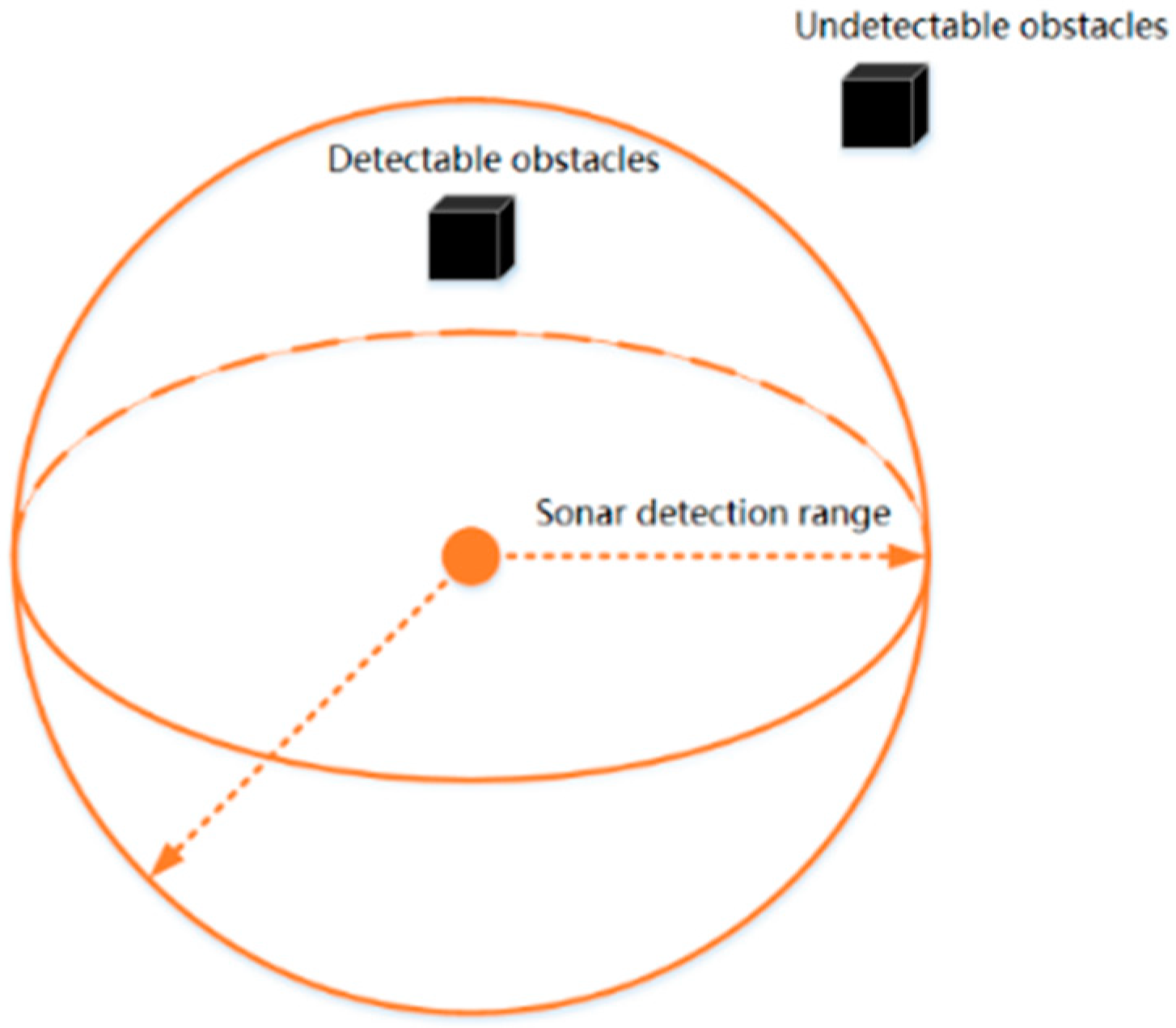
In the above criteria, R is the maximum detection radius of the sonar. In theory, all targets within the AUV’s field of view can be detected. The specific judgment is shown in Figure 3. The sonar can detect environmental information within a spherical range with the AUV as the center and a radius of 100 m. The search for unknown targets is mainly aimed at underwater targets. Therefore, the electronic chart is not suitable for application in this study. The onboard sensor is mainly used in the search for underwater targets. Due to blurred vision in underwater environments, it is more suitable to search with sheet sensors.

2.3. The Environment Model

In this section, the three-dimensional target search area is expanded into a cuboid $\Omega$ of $L_x\times L_y\times L_z$. The target area $\Omega$ is rasterized and divided into $M\times N\times K$ three-dimensional actual grids of size $100 \mathrm{m}\times 100 \mathrm{m}\times 100 \mathrm{m}$. In this section, a set (4) is used to express the target area.

$$TA=\left\{\left(m,n,k\right)|m=1,2\dots M,n=1,2\dots N,k=1,2\dots K\right\}.$$

(4)

In the above set, grid $\left(m,n,k\right)$ represents the $k+\left(n-1\right)\times N+\left(m-1\right)\times M$ grid starting from the origin. In this study, there are only two kinds of grid states: target exists in the grid and target does not exist in the grid, and there is at most one target in each grid. The grid state is represented by ${\delta }_a$, and its state is represented by Equation (5).

$${\delta }_a=\{\begin{array}{l}0, \mathrm{When} \mathrm{there} \mathrm{is} \mathrm{a} \mathrm{target} \mathrm{in} \mathrm{grid} a\\ 1, \mathrm{When} \mathrm{there} \mathrm{is} \mathrm{no} \mathrm{target} \mathrm{in} \mathrm{grid} a\end{array},$$

(5)

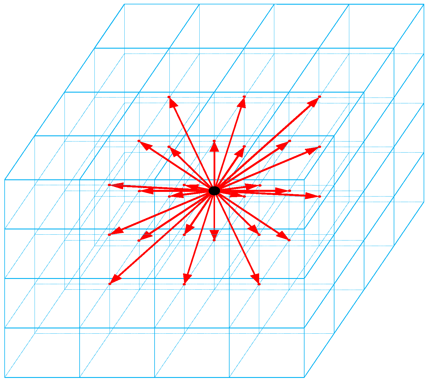
2.4. AUV Movement Direction

In a grid diagram, the AUV can move to the grid adjacent to the current grid, but cannot move back to the grid of the previous moment. The discretization diagram of its motion direction is shown in Figure 4.

3. Modeling and Updating of Real-Time Perception Map

The real-time perception map represents the AUV’s awareness of the target search environment. As the AUV explores the search environment, the AUV obtains real-time detection information of the surrounding environment through its own sensors, and updates the real-time perception map. Then, search performance gains are formulated based on real-time perception maps. According to the improvement of the search performance, the best search position is determined at the next moment, and the above steps are continuously executed in a loop until all targets are found or the estimated search time is over. In this section, real-time perception maps include models such as target existence probability maps, uncertainty maps, revisited pheromone maps, attraction source maps, and search status maps.

3.1. Target Existence Probability Map

The target existence probability map represents the probability of the target’s existence in the actual grid. Each grid has its target existence probability at different moments [18]. For example, the probability of the actual target in grid $a$ at time K can be expressed by $p_a\left(k\right)$, $p_a\left(k\right)ϵ\left[0,1\right].$ $p_a\left(k\right)$ = 1 represents that the AUV believes that there is a target in grid a at the moment k. Similarly, $p_a\left(k\right)=0$ represents that the AUV believes that there is no target in grid $a$ at the moment k. Since the AUV searches in an unknown underwater environment, the AUV knows nothing about the target position, obstacle position, and other information in the entire mission area before searching, namely, $p_a\left(0\right)=0.5$. $p_a\left(0\right)$ represents the probability of the existence of the target in grid $a$ before the mission begins. At that time, the AUV considers the “possibility of the target’s existence” and the “possibility of the target’s nonexistence” in grid $a$ to be exactly the same.

The target existence probability map of the AUV can be defined as:

$$M_{TPM}\left(k\right)=\left\{p_a\left(k\right)|a\in \Omega \right\}.$$

(6)

In the process of underwater target searches, the AUV will update the target existence probability graph in real time according to the surrounding environment information detected by the sensor. Due to the limited detection range of the sensor, only the target existence probability of the grid within the detection range of the AUV sensor needs to be updated, and the target existence probability of other grids remains unchanged.

Due to the influence of noise and other factors, the sensor mounted on the AUV may miss the target or identify a target in a grid that does not exist. Detection probability $p_d$ is the probability that the sensor finds a target in the grid where the real target exists. False alarm probability $p_f$ is the probability that the sensor detects a target in a grid where there is no real target. Detection probability $p_d$ and false alarm $p_f$ reflect the performance of the sensor. $det(a,k)$ is used to represent the event that the sensor equipped on AUV detects the presence of a target in grid $a$ at the time of k; $real\left(a\right)$ is used to represent the event that the target really exists in grid $a$; then $p_d$ and $p_f$ can be represented by Equations (7) and (8).

$$p_d=p\left(det(a,k\right)|real\left(a\right)),$$

(7)

$$p_f=p\left(det(a,k\right)|\overline{real\left(a\right)}),$$

(8)

$$\overline{p_d}=p(\overline{det(a,k)}|real\left(a\right)),$$

(9)

$$\overline{p_f}=p\left(\overline{det(a,k)}|\overline{real\left(a\right)}\right).$$

(10)

In the above formula, $p_d$ represents the detection probability, $p_f$ represents the false alarm probability, $\overline{p_d}$ represents the probability of the event “sensor fails to detect $a$ target in the grid where there is a real target”, and $\overline{p_f}$ represents the probability of the event “sensor fails to detect a target in the grid where there is no real target”.

The target existence probability map is actually updated according to the posterior probability determined by the detection results of the grid at the previous moment and the current moment by the AUV. In Equation (11), the target existence probability update formula of grid $a$ at time $k$ + 1 when assuming that the AUV detects the existence of a target in grid $a$ at time $k$ + 1 is shown.

$$p_{a,k+1}=\frac{p_d·p_{a,k}}{p_d·p_{a,k}+p_f·\left(1-p_{a,k}\right)}.$$

(11)

In Equation (12), the target existence probability update formula of grid $a$ at time $k$ + 1 when assuming that the AUV detects no target in grid $a$ at time $k$ + 1 is shown.

$$p_{a,k+1}=\frac{\left(1-p_d\right)·p_{a,k}}{\left(1-p_d\right)·p_{a,k}+\left(1-p_f\right)·\left(1-p_{a,k}\right)}.$$

(12)

The target existence probability of the grid outside the sonar detection range at time $k$ + 1 is the same as that at time K, which means $p_{a,k+1}=p_{a,k}$.

It is known from the literature [10] that when $0<p_f<0.5<p_d<1$, and the more AUV probes in grid $a$, the more accurate the AUV’s judgment on whether there is an actual target in grid $a$ will be, which proves the rationality of the existence probability of the target.

When a suspected target is detected in grid $a$, the AUV can quickly determine whether the target exists by approaching the suspected target. Therefore, it is assumed that the AUV approaches the suspected target in grid $a$ at time $k$. If it is determined that the suspected target is a real target in grid $a$, the target existence probability of grid a is $p_{a,k+i}\left(i=1,2,3,\dots \right)=1$. If the suspected target is not a real target, the target existence probability of grid $a$ at time k is recalculated according to the situation that the AUV detects that there is no target in grid $a$ at time $k$ − 1. The calculation formula is shown in Formula (13):

$$p_{a,k}=\frac{\left(1-p_d\right)·p_{a,k-1}}{\left(1-p_d\right)·p_{a,k-1}+\left(1-p_f\right)·\left(1-p_{a,k-1}\right)}.$$

(13)

The convergence speed of the target existence probability in the grid is proportional to the increased speed of the AUV in the detection times of the grid, and the proportional relation between the two is related to the performance of the sensor. The greater the ratio of detection probability $p_d$ to false alarm probability $p_f$, the faster the target existence probability converges with the detection times of the grid. Considering the time of search and rescue missions and the fuel energy of the AUV, this study considers the lower limit $p_{min}$ of the target existence probability. When the probability of the existence of the target in grid a $p_{a,k}<p_{min}$, it is considered that there is no target in task grid $a$. The selection of $p_{min}$ depends on the specific requirements of the search task. Consider that the detection range of sonar is 100 m and the grid side length in this study is 100 m. Since the AUV can determine whether it is a real target by approaching the suspected target, the AUV can reach the suspected target and confirm the target by updating the target existence probability of grid $a$ at most once after finding the suspected target. Therefore, there is an upper limit $p_{max}$ for the target existence probability of $a$:

$$p_{max}=0.5\times {\frac{p_d}{0.5\times p_d+0.5\times p_f}}_{max}.$$

(14)

Therefore, the probability of the existence of the target is either $p_{a,k}\le p_{max}$ or $p_{a,k}=1$.

In order to facilitate the operation, this section shows the transformation of the target existence probability updating formula into linear form by nonlinear transformation. The nonlinear transformation formula is shown in Equation (15).

$$Q_{a,k}\stackrel{\Delta }{=}ln(\frac{1}{p_{a,k}}-1).$$

(15)

In Equation (16), the updating formula of the existence probability of a linear target in grid $a$ at time $k$ + 1 after the nonlinear transformation, if the AUV detected the existence of a target in grid a at time $k$ + 1, is shown.

$$Q_{a,k+1}=Q_{a,k}+ln\frac{p_f}{p_d}.$$

(16)

In Equation (17), the updating formula when assuming that the AUV detects that there is no target in grid $a$ at the time of $k$ + 1 is shown.

$$Q_{a,k+1}=Q_{a,k}+ln\frac{1-p_f}{1-p_d}.$$

(17)

The probability of the existence of the target outside the sonar detection range is constant. According to the above formula after linear change, if there is no target in grid a, when the number of AUV probes in grid $a$ approaches infinity, $Q_{a,k}\to +\infty ,p_{a,k}\to 0$.

3.2. Uncertainty Map

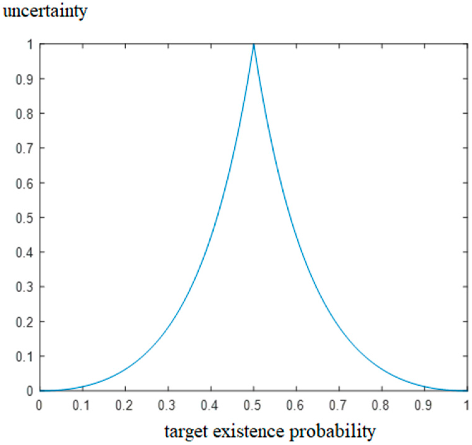
When $p_{min}<p_{a,k}<p_{max}$, whether there is a target in grid a cannot be accurately judged, so an uncertainty map is created to reflect the AUV’s understanding of the grid in the target search area. The uncertainty of the grid is calculated according to the target existence probability. The specific calculation formula is shown in Equation (18).

$${\mu }_{a,k}=e^{-k·\left|Q_{a,k}\right|}.$$

(18)

In the equation above, k is a constant. Combining Equation (15), the relationship between uncertainty and target existence probability is shown in Equation (19).

$${\mu }_{a,k}={(e^{\left|Q_{a,k}\right|})}^{-k}.$$

(19)

As shown in Figure 5, when the target existence probability of grid $a$ is 0.5, the uncertainty of grid $a$ is 1. That means the AUV has no knowledge of the target existence in grid $a$ at all. The greater the difference between the existence probability of the target of grid $a$ and 0.5, the lower the uncertainty of grid $a$. As the AUV visits the grid, the target existence probability of the grid will increase or decrease. The judgment of whether there is a target in the grid will also become more and more accurate as the number of visits increases. When the target existence probability is 0 or 1, the AUV has completely determined the existence of the target in grid a, so the uncertainty of grid a is 0. The purpose of this algorithm is to reduce the uncertainty of the entire search area, so as to ensure the efficiency of the search.

3.3. Attraction Source Map

This section shows an attraction source map used in order to make it easier for the AUV to search for targets that may exist in the corners. In the middle and late stages of the search task, AUVs are attracted to explore the corner areas with low search coverage, thereby improving the efficiency of target exploration.

The mechanism of the attraction source is to set eight attraction sources to be activated with a certain distance from the boundary of the search area at the eight diagonal corners of the search area. The influence range is a spherical area with the attraction source to be activated as the center of the sphere and a radius of 200 m. After calculating the searched coverage rate within the influence range of each attraction source to be activated, the active attraction source can be selected according to the searched coverage rate. The position of the attraction source to be activated in the grid map is shown in Equation (20).

$$ATT=\left\{\left(m,n,k\right)|m=2,M-2;n=2,N-2;k=2,K-2;\right\}.$$

(20)

In the equation above, M, N, K represent the length, width, and height ranges of the grid map of the search area.

The activation conditions of the attraction source are as follows: First, the number of unsearched grids in the range centered on each attraction source in the grid graph is compared. If the number of unsearched grids is greater than or equal to 13, the attraction source can be activated. Then, from the activatable attraction sources, the attraction source with the largest number of unsearched grids around (the lowest search coverage) is selected as the activated attraction source. If there are attraction sources with the same search coverage, the attraction source closer to the current position of the AUV is selected as the activated attraction source.

When the attraction source is activated, only when the number of unsearched grids around the attraction source does not meet the condition will other attraction sources be reactivated. Only one of the attraction sources can be activated at a time. When the eligible attraction source is activated, the attraction source will diffuse the attraction element to the surroundings. Additionally, the attraction element in the grid will only be updated when a new attraction source is activated or the activated attraction source does not meet the activation conditions.

Considering the above conditions, this section introduces the shunt formula of the neural excitation network algorithm as the diffusion formula of the attraction element. It not only achieves the purpose of spreading the attraction element to the surrounding grid of the attraction source in the direction of the gradient, but also takes the distance between grids into consideration when the attraction element is spreading.

Before the search task starts, since the AUV is not aware of all the grids in the search area, the attraction elements of all the grids are initialized as 0. When a new attraction source is activated, the attraction elements of all grids are first reset to 0, and then the attraction element of the grid where the activated attraction element is located is initialized to an initial value. The attraction pheromone diffuses to the surrounding grid where the attraction source is located in the direction of the gradient. The AUV will have a tendency to move to the surrounding grid with more attraction elements, and will be guided to the corner area where the activated attraction source with low search coverage is located. The change rule of the attraction element in the grid map of the search area is shown in Equation (21).

$$\frac{d{u}_k}{dt}=-A{u}_k+\left(B-u_k\right)([I_k{]}^{+}+{\displaystyle \sum }_{0<\left|kl\right|<\sqrt{3}}{w}_{kl}{[u_l]}^{+}).$$

(21)

In the equation above, $u_k$ represents the attraction element of grid $k$. A and B are constants, A reflects the attenuation rate of attraction elements of grid $k$, and B is the upper limit of attraction elements of grid $k$. $I_k$ is short for input, meaning that the kth neuron receives external input influenced by the activity values of other neurons. ${[I_k]}^{+}$ represents the positive input, or incentive input, received by the KTH neuron. $\left|kl\right|$ represents the distance between neuron k and neuron $l$. $w_{kl}$ represents the neuron connecting weight coefficient between neuron k and neuron $l$. When there is a connection between neuron k and neuron $l$, $w_{kl}=\mu /\left|kl\right|$. $\mu$ is a constant coefficient, usually between 0 and 1. When there is no connection between neuron $k$ and neuron $l$, $w_{kl}=0$. ${[u_l]}^{+}$ represents the positive input of neurons around neuron $k$ to neuron $k$, namely, the sum of the positive neuron activity of all neurons around neuron $k$. $\sum _{0<\left|kl\right|<r_o}{w}_{kl}{[u_l]}^{+}$ represents the sum of the positive excitation of the peripheral neurons whose distance from the neuron $k$ position is not greater than $r_o$. $r_o$ is a constant, generally set as the furthest Euclidean distance between the AUV and the surrounding grid.

Considering the magnitude of the uncertainty in this section, when the attraction source is activated, the attraction element of the grid where the attraction source is activated to 3, and the attenuation rate of the attraction element is set to a small value. Since there are many surrounding grids of a grid in a three-dimensional environment and the upper limit set of the attraction element is large, the sum of the positive excitations given by the surrounding grids is large, so the value of $\mu$ needs to be small, thereby ensuring that the attraction element descends according to the gradient. In the diffusion formula of the attraction element, the parameters are set as $A=0.01,B=3,\mu =0.15$.

3.4. Revisit Pheromone Map

The main task of the AUV in the early stage of the search task is to reduce the uncertainty of the entire search environment. However, when most areas in the search environment have been searched, there may be targets in the searched grid area that have not been detected due to the performance of the sonar carried by the AUV. Therefore, we designed a revisit pheromone map. In the later stage of the search, the AUV is guided to revisit the area in the search environment that meets the specific rules. The purpose is to prevent the target in the searched grid from not being detected due to the detection performance of the sonar, thereby improving the search efficiency.

The following conditions must be met for the grid to release the revisited pheromone:

1. Set a revisit time $T_v$. If grid a is revisited at time k, then from time k to time $k+T_v$, grid a will not be revisited, and no revisited pheromone will be released.

2. The target existence probability of grid a at time k can only be released if Equation (22) is satisfied.

$$\frac{\left(1-p_d\right)·\frac{\left(1-p_d\right)}{\left(1-p_d\right)+\left(1-p_f\right)}}{\left(1-p_d\right)·\frac{\left(1-p_d\right)}{\left(1-p_d\right)+\left(1-p_f\right)}+\left(1-p_f\right)·\left(1-\frac{\left(1-p_d\right)}{\left(1-p_d\right)+\left(1-p_f\right)}\right)}\le p_{a,k}<0.5.$$

(22)

Compared with other grids, the number of instances of detection by the AUV is less than or equal to twice. In addition, due to the detection efficiency of the sensor, the grid that results in no target will be missed every time. Therefore, the AUV needs to revisit the grid that meets these conditions, so as to solve the problem that the target may exist but has not been detected more quickly in the later stage of the search and improve the efficiency of search.

Since the release mechanism of revisited pheromone is similar to that of the attraction element, the updating formula of revisited pheromone is the same as shown in Equation (21). A certain revisited pheromone is initialized in a grid meeting the revisited pheromone release conditions, and the revisited element is diffused to the surrounding grid in the direction of the gradient. Revisited pheromone only works when map coverage is high. In this section, the parameters of the revisited pheromone diffusion formula are set as: $A=0.2,B=1,\mu =0.1$.

3.5. Search Status Map

In order to distinguish the areas that the AUV has searched, and guide the AUV to search the unexplored areas, a search status map was designed. The search status map can be expressed by Equation (23).

$$Searched=\left\{\left(a,b,c\right)|a=1,2\dots M,b=1,2\dots N,c=1,2\dots K\right\}.$$

(23)

There are only two states of the search grid in this article: the grid has been searched and the grid has not been searched. Before the search task starts, the states of all grids in the search status map are unsearched. The grid within the detection range of the AUV sonar is regarded as a searched grid. The search state of grid a can be represented by $S_a$, and its state is shown in Equation (24).

$$S_a=\{\begin{array}{l}0, \mathrm{Grid} a \mathrm{is} \mathrm{not} \mathrm{searched} \\ 1, \mathrm{Grid} a \mathrm{has} \mathrm{been} \mathrm{searched} \end{array}.$$

(24)

4. Search Decision

4.1. Search Performance Gain Function

This study considers the following aspects in search decisions:

• Search the area that can reduce the uncertainty quickly;
• Search the unsearched grids as far as possible;
• Search corner areas with low search coverage in the middle stage of the search;
• Try to revisit the area with a high element level in the later stage of the search, so as to avoid the situation that the target is not detected due to the performance of the sensor;
• Minimize the large steering of the AUV.

This section describes the five aspects of uncertainty gains, attract prime gains, steering costs, exploration gains and revisit pheromone gains, and design of the search performance gain function. The AUV can use the target search performance gain function to evaluate the position of the AUV at the next moment through the target search revenue function, and select the grid with the largest target search performance gain as the next search mobile decision point. Assuming that the AUV is in the grid pre at time $k$ − 1, the AUV can move to the grid adjacent to grid pre at time $k$. In Equation (25), the specific formula of the search performance gain function, assuming that the AUV plans to go from grid pre to grid a at time k (grid a is the grid adjacent to grid pre where the AUV is currently located), is shown.

$$\begin{array}{l}INC\left(a,k\right)\\ =\{\begin{array}{l}0.6·I_A\left(a,k\right)+0.1·I_B\left(a,k\right)-0.2·I_C\left(a,k\right)+0.1·I_D\left(a,k\right),cov(k)<50\%\\ 0.4·I_A\left(a,k\right)+0.2·I_B\left(a,k\right)-0.1·I_C\left(a,k\right)+0.4·\left(1+cov(k\right))·I_D\left(a,k\right)+0.1·I_E\left(a,k\right),cov(k)\ge 50\%\\ 0.4·I_A\left(a,k\right)+0.3·I_B\left(a,k\right)+0.4·\left(1+cov(k\right))·I_D\left(a,k\right)+0.3·I_E\left(a,k\right),cov(k)\ge 80\%\end{array}\end{array}$$

(25)

In the equation above, $I_A\left(a,k\right)$ represents the uncertainty gains that the AUV can obtain when going to grid a at time k. $I_B\left(a,k\right)$ represents the exploration gains that the AUV can obtain, that is, the gains of a nonrepetitive search. $I_C\left(a,k\right)$ represents the steering cost of the AUV. $I_D\left(a,k\right)$ represents the attraction element gains. $I_E\left(a,k\right)$ represents the revisited pheromone gains that the AUV can obtain when going to grid a at time $k$. $cov(k)$ represents the search coverage of the entire environment at time $k$, that is, the proportion of searched grids in all grids.

The search decision function can be formed by constructing different maps, which can prevent the AUV from making different decisions according to different periods in the search process. In the early stage of the search, the uncertainty map is used to reduce the uncertainty of the environment. In the middle of the search, the AUV will search more corner areas by attracting pixel maps. In the later stage of the search, the AUV repeats the search by revisiting the map to find missing targets from the previous search process.

The weight coefficient of each gain is set according to the task requirements. In the early stage of the search, the weight coefficient of A will be very large, and in the middle and late stages of the search, the weight coefficient of the replay pheromone will be very large. In the early stages of the search, the main purpose of the AUV is to reduce the uncertainty of the entire environment. Since the uncertainty gain occupies a relatively high proportion, the weight coefficient of A will be very large in the early stage of the search. In the middle and late stages of the search, due to the detection efficiency of the sensor, it is necessary to guide the AUV to search for corner areas that have not been searched and grid areas that may have missed targets. In addition, the grids that have been explored should be explored as little as possible, so the income of revisiting pheromone and the income of attractive elements has begun to occupy a certain proportion of the search income function, and the proportion of exploration income has increased. Therefore, in the middle and late stages of the search, the weight coefficient of the replay pheromone will be very large. If the AUV uses the search performance gain function to determine the next optimal search position decision, and an obstacle is detected at that position, the search performance gain of the grid is set to 0, and then the optimal position decision is re-determined.

4.2. Search Revenue Composition

The search gain function predicts the maximum gain of the AUV search at the next moment based on the real-time environment map at the current moment. The uncertainty gain $I_A\left(a,k\right)$ is the sum of the uncertainty of all the grids in the detection region with the sensor detection range as the radius centered on grid $a$ at the moment $k$ − 1. It is expressed by Equation (26).

$$I_A\left(a,k\right)={\displaystyle \sum }_{b\in \varphi \left(a\right)}\mu \left(b,k-1\right).$$

(26)

$\varphi \left(a\right)$ is the detection target surface of grid a, that is, all grids in the detection area with grid a as the center and the detection range of the sensor as the radius.

The exploration gain $I_B\left(a,k\right)$ is the ratio of the unsearched grids in the range of the sensor to all grids in the range of the sensor at time $k$ − 1, as shown in Equation (27).

$$I_B\left(a,k\right)=\frac{{\sum }_{b\in \varphi \left(a\right)}{S}_b\left(k-1\right)}{N\left(b\right)}.$$

(27)

$S_b\left(k-1\right)$ is the grid search state of grid $b$ in the searched map at time k − 1, ${\sum }_{b\in \varphi \left(a\right)}{S}_b\left(k-1\right)$ is the sum of the unsearched grids within the sensor scope of grid $a$, and $N\left(b\right)$ is the total number of grids within the sensor scope of grid $a$.

The steering cost $I_C\left(a,k\right)$ depends on whether the AUV’s next action is executed on the same course as the current course. If it is the same, then $I_C\left(a,k\right)=0$, or $I_C\left(a,k\right)=1$.

Attraction element yield $I_D\left(a,k\right)$ is determined according to whether the attraction source is activated or not. If an attraction source is activated, attraction element yield $I_D\left(a,k\right)=att\left(a,k-1\right)$, where $att\left(a,k-1\right)$ represents the attraction element content in grid a at time k − 1. If no attraction source is activated, then $I_D\left(a,k\right)=0$.

The revisited element yield is the revisited element content in grid a at the moment k − 1.

$$I_E\left(a,k\right)=v\left(a,k-1\right),$$

(28)

where $v\left(a,k-1\right)$ is the pheromone content of grid $a$ at time $k$ − 1.

5. Path Planning

When the AUV determines the next search location decision according to the search performance gain function or detects a suspicious target near it through sonar, it needs to use the path planning method to reach the decision location or the suspect target. Therefore, while planning the search path through the above search algorithm in real time, this study also considers the rotation angle limit of the AUV, and designs an improved neural excitation network algorithm to plan the navigation path of the AUV to make it more in line with the actual search situation of the AUV.

5.1. Angle Constraint of AUV

Considering the kinematic characteristics of the AUV, the AUV has limitations on the steering angle of the course angle and the angle change in the vertical direction [20]. Since the AUV runs in a three-dimensional environment and involves search problems in different water depths, the AUV used in this study is equipped with auxiliary propellers that can move in the vertical direction at different water depths.

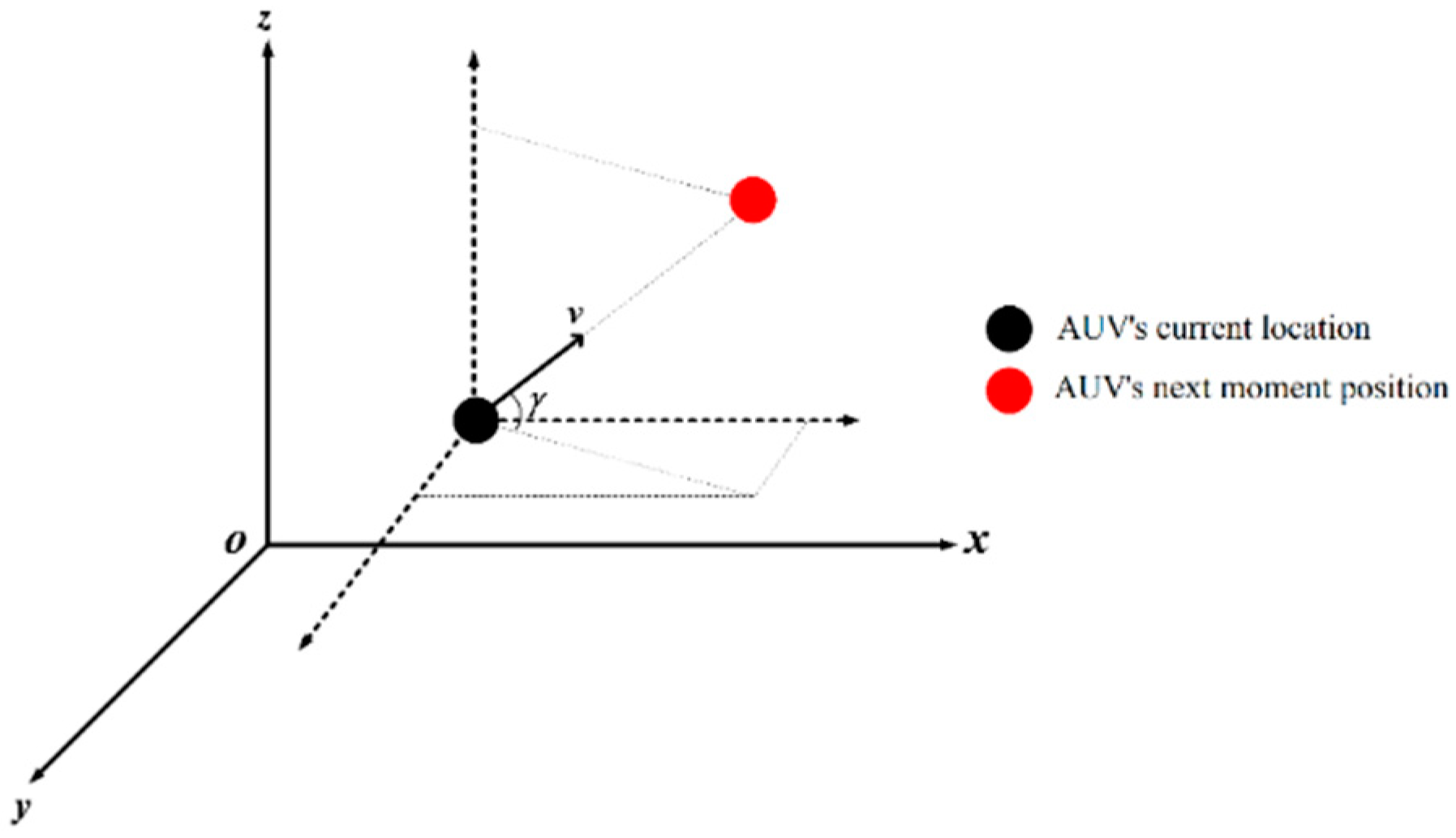
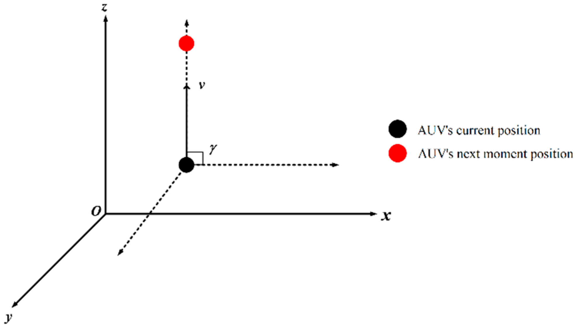
As shown in Figure 6 and Figure 7, the AUV can calculate the predicted speed direction of the AUV at the current position through the current position and the position at the next moment. In this study, the speed of the AUV is set to 2 m/s. The angle $\gamma$ between the predicted speed and the $xoy$ plane must meet the following conditions: $\left|\gamma \right|\le {30}^{\circ }$ or $\left|\gamma \right|={90}^{\circ }$. If ${30}^{\circ }<\left|\gamma \right|<{90}^{\circ }$, according to the current position of the AUV $\left(x_0,y_0,z_0\right)$ and the position of the next moment $\left(x,y,z\right)$, the rise and fall judgment will be made: when $z>z_0$, the AUV will move upward at a fixed speed in the vertical direction until the angle $\gamma$ meets the condition. When $z<z_0$, the AUV moves downward at a fixed speed in the vertical direction until the angle $\gamma$ meets the condition.

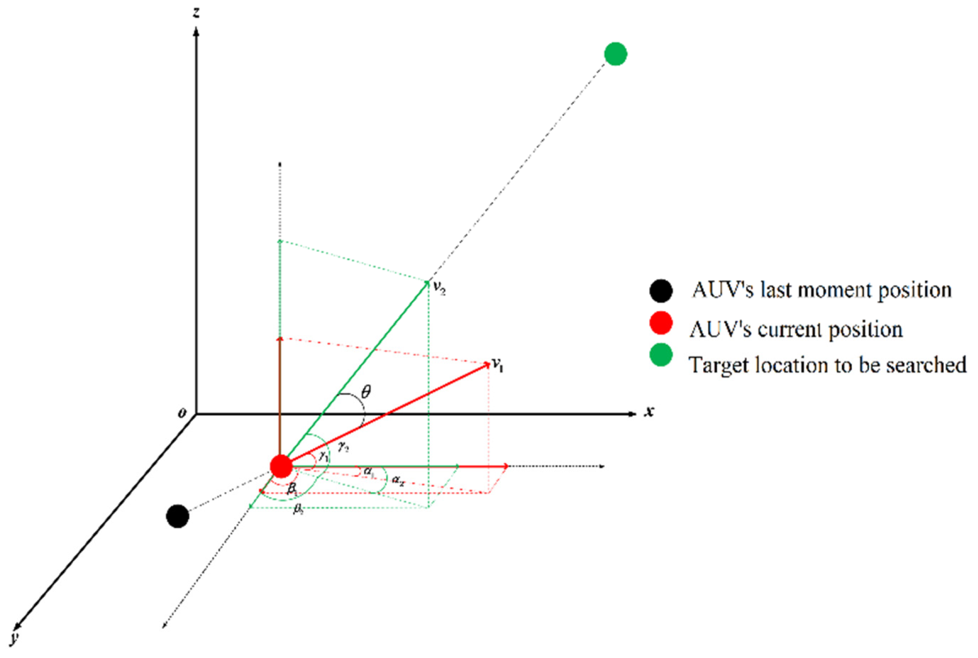
On the basis that the AUV satisfies the motion conditions on the z-axis, the rotation angle limit of the course angle is also considered. The schematic diagram of the angle is shown in Figure 8.

The speed direction $v_1$ of the AUV at the current position can be calculated by the position of the last step of the AUV and the current position of the AUV, and the expected speed direction $v_2$ of the AUV can be calculated by the current position of the AUV and the target position for the AUV to search. The angle $\theta$ between $v_1$ and $v_2$ is calculated according to the relative positions between the three. The speed of the AUV’s position at the next moment is set as $v_0$, then $v_0$. satisfies the condition of Formula (29):

$$\{\begin{array}{l}{v}_0=v_2, \theta \le {30}^{\circ }\\ v_0=v_1+\Delta v, \theta >{30}^{\circ }\end{array}.$$

(29)

In other words, the meaning of Equation (29) is that when the expected turning angle $\theta$ is less than or equal to 30 degrees, the turning can be carried out directly; when $\theta$ is greater than 30 degrees, a small angle is needed for gradual turning.

The size of $\Delta v$ is two meters, which is the distance the AUV can move in one second. The angle $\Delta \alpha$ between the component of $\Delta v$ on the $xoy$ plane and the x-axis satisfies the condition of Equation (30).

$$\Delta \alpha =\{\begin{array}{l}{10}^{\circ }, \left|{\alpha }_2-{\alpha }_1\right|\ge {10}^{\circ }\\ \frac{\left|{\alpha }_2-{\alpha }_1\right|}{10}, 0^{\circ }<\left|{\alpha }_2-{\alpha }_1\right|<{10}^{\circ }\\ 0^{\circ }, \left|{\alpha }_2-{\alpha }_1\right|=0^{\circ }\end{array},$$

(30)

where ${\alpha }_1$ is the angle $v_1$ between the component on the $xoy$ plane and the x-axis, and ${\alpha }_2$ is the angle between the component of $v_2$ on the $xoy$ plane and the x-axis. The angle $\Delta \beta$ between the component of $\Delta v$ on the $xoy$ plane and the y-axis and the angle $\Delta \gamma$ between $v_1$ and the $xoy$ plane are calculated in the same way, as shown in Equations (31) and (32).

$$\Delta \beta =\{\begin{array}{l}{10}^{\circ }, \left|{\beta }_2-{\beta }_1\right|\ge {10}^{\circ }\\ \frac{\left|{\beta }_2-{\beta }_1\right|}{{10}^{\circ }}, 0^{\circ }<\left|{\beta }_2-{\beta }_1\right|<{10}^{\circ }\\ 0^{\circ }, \left|{\beta }_2-{\beta }_1\right|=0^{\circ }\end{array},$$

(31)

where ${\beta }_1$ is the angle between the component of $v_1$ on the $xoy$ plane and the y-axis, and ${\beta }_2$ is the angle between the component of $v_2$ on the $xoy$ plane and the y-axis.

$$\Delta \gamma =\{\begin{array}{l}{5}^{\circ }, \left|{\gamma }_2-{\gamma }_1\right|\ge 5^{\circ }\\ \frac{\left|{\gamma }_2-{\gamma }_1\right|}{5^{\circ }}, 0^{\circ }<\left|{\gamma }_2-{\gamma }_1\right|<5^{\circ }\\ 0^{\circ }, \left|{\gamma }_2-{\gamma }_1\right|=0^{\circ }\end{array},$$

(32)

where ${\gamma }_1$ is the angle between plane $v_1$ and $xoy$, and ${\gamma }_2$ is the angle between plane $v_2$ and plane $xoy$.

In this study, based on the artificial potential field method to calculate the gravitational direction of the AUV at each moment, the gravitational direction is combined with the above velocity direction, so that the planned path can meet the kinematic limitation of the AUV.

5.2. Improved Artificial Potential Field Method

The artificial potential field method constructs a virtual potential field in the search area. The potential field consists of two different potential fields: gravitational potential field and repulsive potential field. The target point generates gravity on the AUV through the gravitational potential field, and the obstacle generates repulsion on the AUV through the repulsive potential field. The direction of gravitation is directed from the AUV to the target point, and the direction of repulsion is directed from the obstacle to the AUV. Finally, the AUV moves to the target through the combined force of the received forces [21]. The advantage of the artificial potential field method is that the amount of calculation is small, and the planned path is safer and smoother, but it is easy to fall into the local optimum.

The focus of the artificial potential field method is the construction of the gravitational potential function and the repulsive potential function [22]. The construction of the gravitational potential function is related to the Euclidean distance between the target and the AUV. The farther the AUV is from the target, the greater the gravitational force it receives. When the AUV reaches the target, the gravitational force on the AUV is zero. The gravitational potential function in this study is shown in Formula (33).

$$U_{att}\left(q\right)=\frac{1}{2}\times k_{att}\times {(X-X_g)}^2,$$

(33)

where $k_{att}$ is the scale factor of the gravitational function, which is a constant. $\left|X-X_g\right|$ represents the Euclidean distance between the target and the current position of the AUV. The magnitude of the gravitational force is the derivative of the gravitational potential field with respect to the distance, and the direction is from the AUV to the target. The specific formula is shown in Equation (34).

$$F_{att}\left(q\right)=k_{att}\times \left|X-X_g\right|.$$

(34)

As the AUV has a rotation angle limit in underwater courses, this study combines the direction of gravity with the speed idea after considering the rotation angle limit to make it conform to the actual navigation situation of the AUV.

The construction of the repulsion potential function is related to the distance between the obstacle and the AUV and the influence range of the obstacle. Within the influence range of the obstacle, the closer the AUV is to the obstacle, the greater the repulsive force it receives. The repulsive force received by the AUV is zero when it is outside the influence range of obstacles.

The traditional artificial potential field method only considers the distance between the AUV and the obstacle material center in the repulsive force formula without considering the actual factors such as the shape of the obstacle and the safety distance of the AUV from the obstacle. Therefore, in this study, by calculating the distance between each corner of the obstacle and the center of gravity, the maximum distance is selected as one of the influencing factors of the repulsion function. The larger the obstacle volumes, the larger the repulsion coefficient is. Therefore, this realizes the safe collision avoidance of the AUV. The improved repulsion potential function is shown in Formula (35).

$$U_{\mathrm{rep}}=\{\begin{array}{l}\frac{1}{2}\times r^{1.3}\times k_{rep}{(\frac{1}{\rho \left(q,q_0\right)}-{\rho }_0)}^2,0\le \rho \left(q,q_0\right)\le {\rho }_0\\ 0, \rho \left(q,q_0\right)>{\rho }_0\end{array},$$

(35)

where r is the maximum distance between the corner of the obstacle and the center of gravity.

6. Target Search Algorithm Flow

The AUV unknown target search algorithm proposed in this paper is mainly divided into two parts: 1. The target search decision-making part. First, establish a real-time perception map, update the real-time perception map according to the environmental information detected by the AUV equipped with sonar, explore the suspected target, and use the search gain function to determine the next decision point. 2. The execution part of path planning. Use the improved artificial potential field method to reach the decision position or suspected target, and avoid obstacles.

The flowchart of the AUV target search algorithm proposed in this paper is shown in Figure 9. The main steps are as follows:

Step 1: Regard the AUV and the target as mass points, and rasterize the search area.

Step 2: Initialize the parameters and the initial position of the AUV. The parameters include the detection probability and false alarm probability of the AUV equipped with a sonar sensor, the activation radius of the attraction source, the parameters in the attraction element and pheromone update formula, etc. Initialize the grid position of the AUV in the grid map.

Step 3. Establish and initialize the real-time perception map. On the basis of the grid map, establish the target existence probability map, the uncertainty map, the revisited pheromone map, the search status map, the attraction source map, and other real-time perception maps, and initialize them.

Step 4. The AUV detects the surrounding environment through its own sonar. If there is no suspected target point in the detection range, skip to Step 6. If there is a suspected target point in the detection range, the AUV will reach the suspected target point by improving the artificial potential field method. After arriving at the suspected target point, update the AUV’s current position status and real-time perception map. Then, confirm whether it is the target to be searched at a close distance through sensors such as an optical camera. If it is a target to be searched, the number of searched targets is increased by 1. Otherwise, the number of searched targets remains unchanged.

Step 5: Determine whether the number of searched targets has reached the total number of expected search targets or whether the search time has reached the specified time. If it has been reached, the task ends, otherwise skip to Step 3.

Step 6: Evaluate the search gain of each grid around the AUV, select the grid with the largest search gain as the next search position of the AUV, and then move to the grid with the largest search gain. Then, update the current state of the AUV, that is, the current grid position of the AUV.

Step 7: Perform a real-time perception map update based on the surrounding environment information detected by the sonar. After the update, jump to Step 3 to perform the algorithm loop.

7. Simulation Research

In this study, the actual size of the search area is set to $800 \mathrm{m}\times 800 \mathrm{m}\times 800 \mathrm{m}$. The detection radius of the sonar sensor is 100 m, the detection probability is $p_d=0.9$, and the false alarm probability is $p_f=0.1$. After rasterizing the search area, the detection range of the AUV’s sonar sensor is $2\times 2\times 2$. In this simulation experiment, the obstacle is expanded into a spherical shape to achieve maximum collision avoidance, and the AUV and target are regarded as mass points. During the operation of the AUV, the AUV’s speed is set to 4 knots (kn), that is, the speed is 2 m/s. In this study, the number of steps is used as the algorithm measurement unit. Considering the speed of the AUV, it is assumed that every two meters of the AUV is one step, and the time for each step is one second.

7.1. Real-Time Perception Map Target Search

In this simulation experiment, the initial coordinate of the AUV is (0,0,0), and the center coordinates of the obstacle and target coordinates are shown in the following table. In the simulation diagram, the target is represented by a five-pointed star, and the obstacle is represented by a black sphere. The center coordinates of obstacles are shown in

Table 1. Obstacle center coordinates.

Obstacle	Obstacle Center Coordinates	Obstacle Radius (m)
Obj1	(30,108,104)	16
Obj2	(52,100,40)	12
Obj3	(564,456,345)	10
Obj4	(324,675,456)	26
Obj5	(630,110,650)	16

. The coordinates of the actual target are shown in

Table 2. Actual target coordinates.

Target	Target Coordinates
Tar1	(608,470,572)
Tar2	(476,169,238)
Tar3	(288,287,652)
Tar4	(134,519,400)
Tar5	(409,370,600)
Tar6	(383,537,341)
Tar7	(169,334,411)
Tar8	(522,260,236)
Tar9	(597,383,325)
Tar10	(355,436,384)
Tar11	(218,605,442)
Tar12	(324,157,326)
Tar13	(145,215,668)
Tar14	(584,174,679)
Tar15	(461,505,245)

.

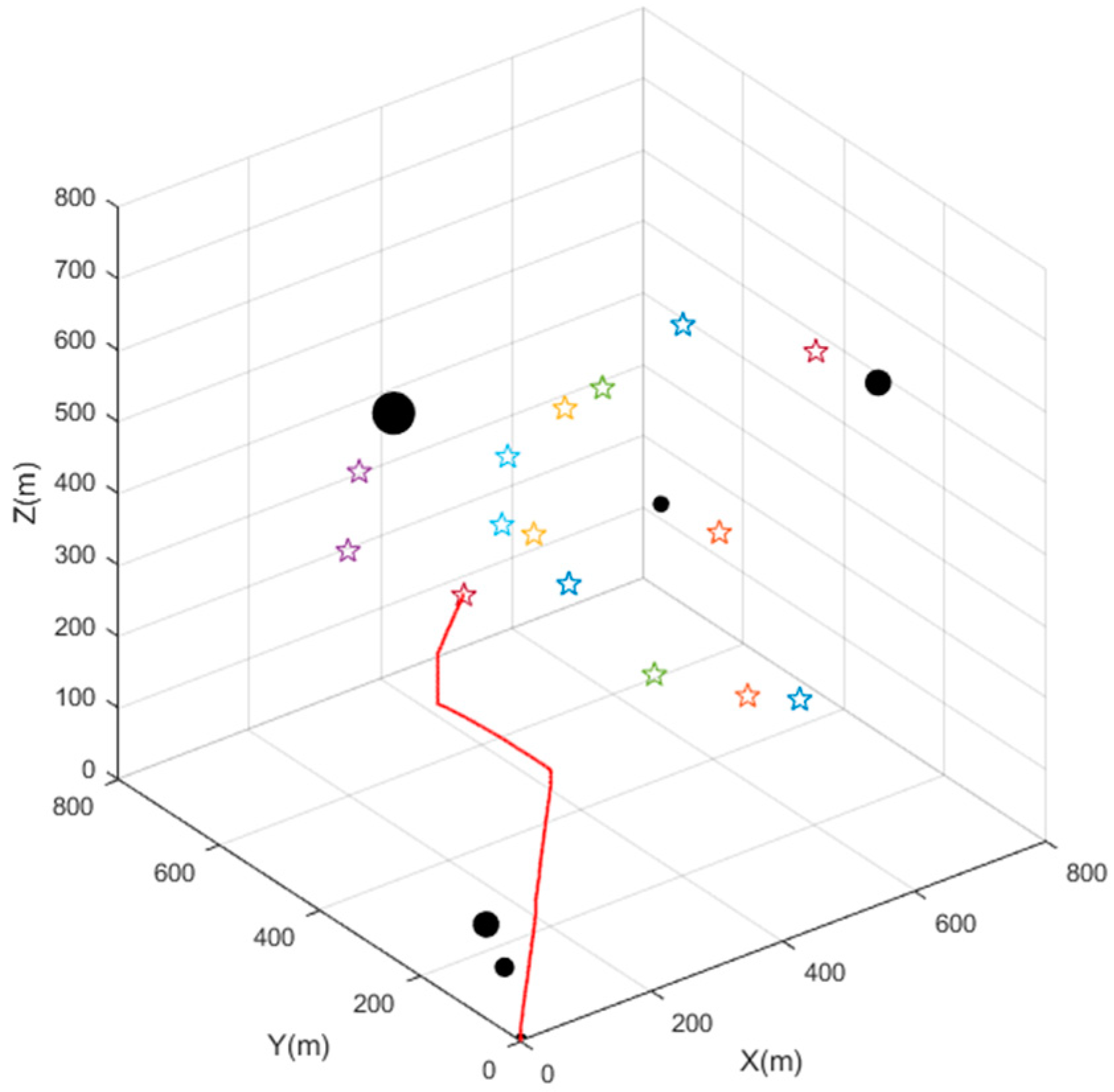
When the AUV is at the starting point, because there is no suspected target within the sonar detection range, the AUV will update the perception map in real time based on the surrounding environment information detected by the sonar. The search gain function is used to make a search position decision, and the AUV navigates to the decision position until a suspected target point appears in the AUV’s detection range. The AUV will approach the suspected target point and use the sensor to confirm the target point at close range as shown in Figure 10. The five-pointed stars of different colors represent different unknown targets which the AUV is searching for, and the black ones represent spherical obstacles.

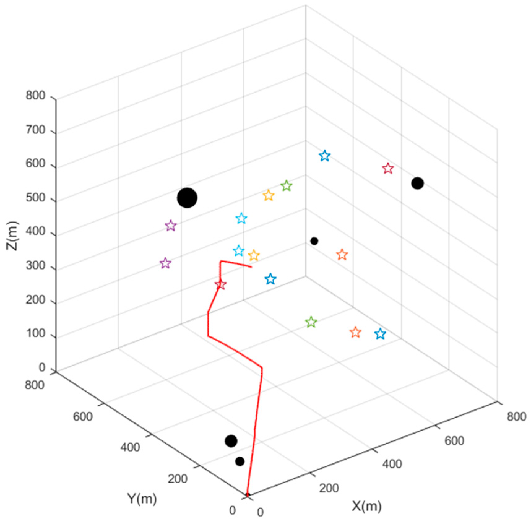
After the AUV judges the suspected target point, if there is no suspected target within the sonar detection range, the perception map will be updated again according to the environmental information within the sonar detection range. The AUV makes search location decisions based on the search gain function, as shown in Figure 11, until the suspected target reappears in the sonar detection range.

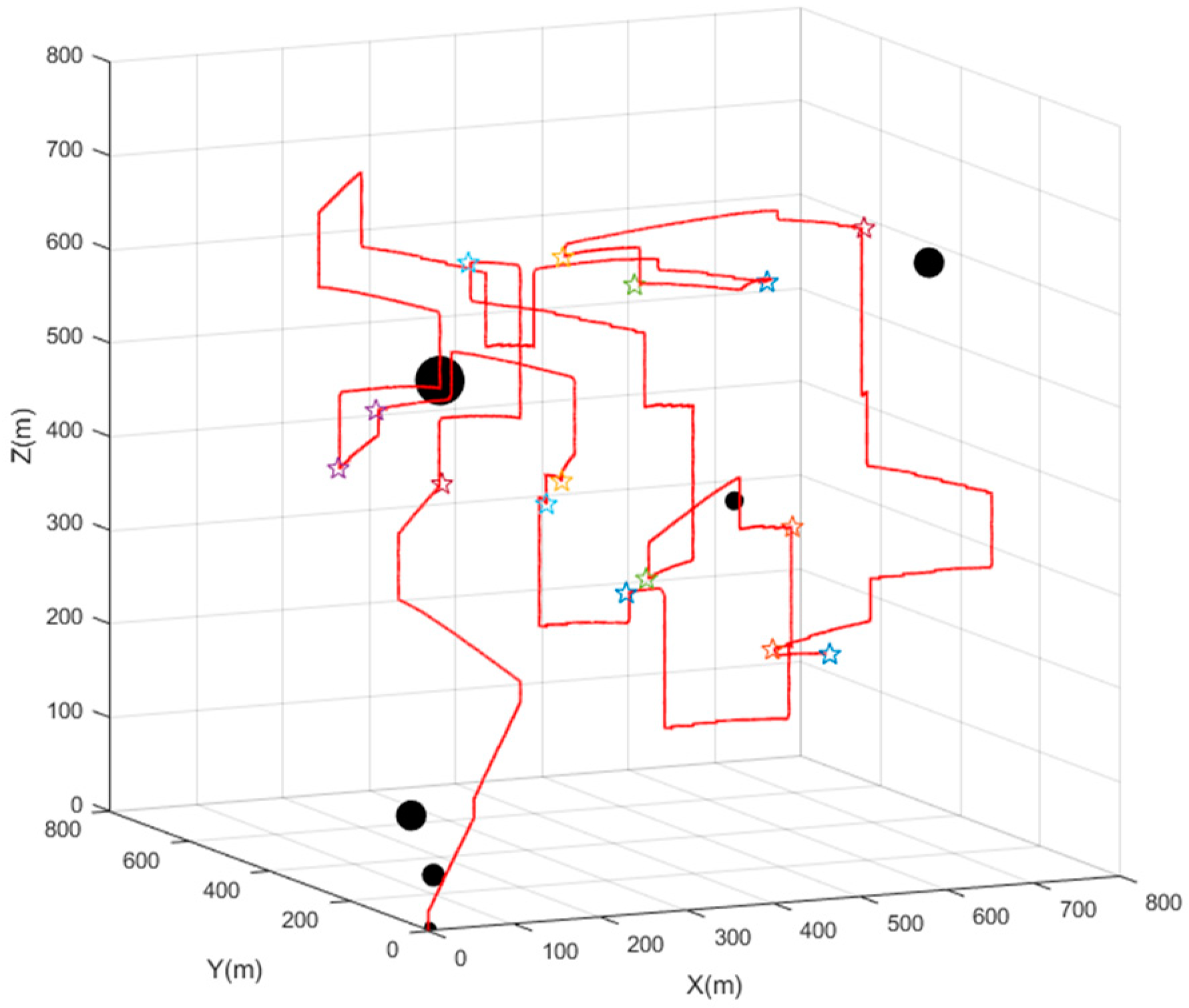
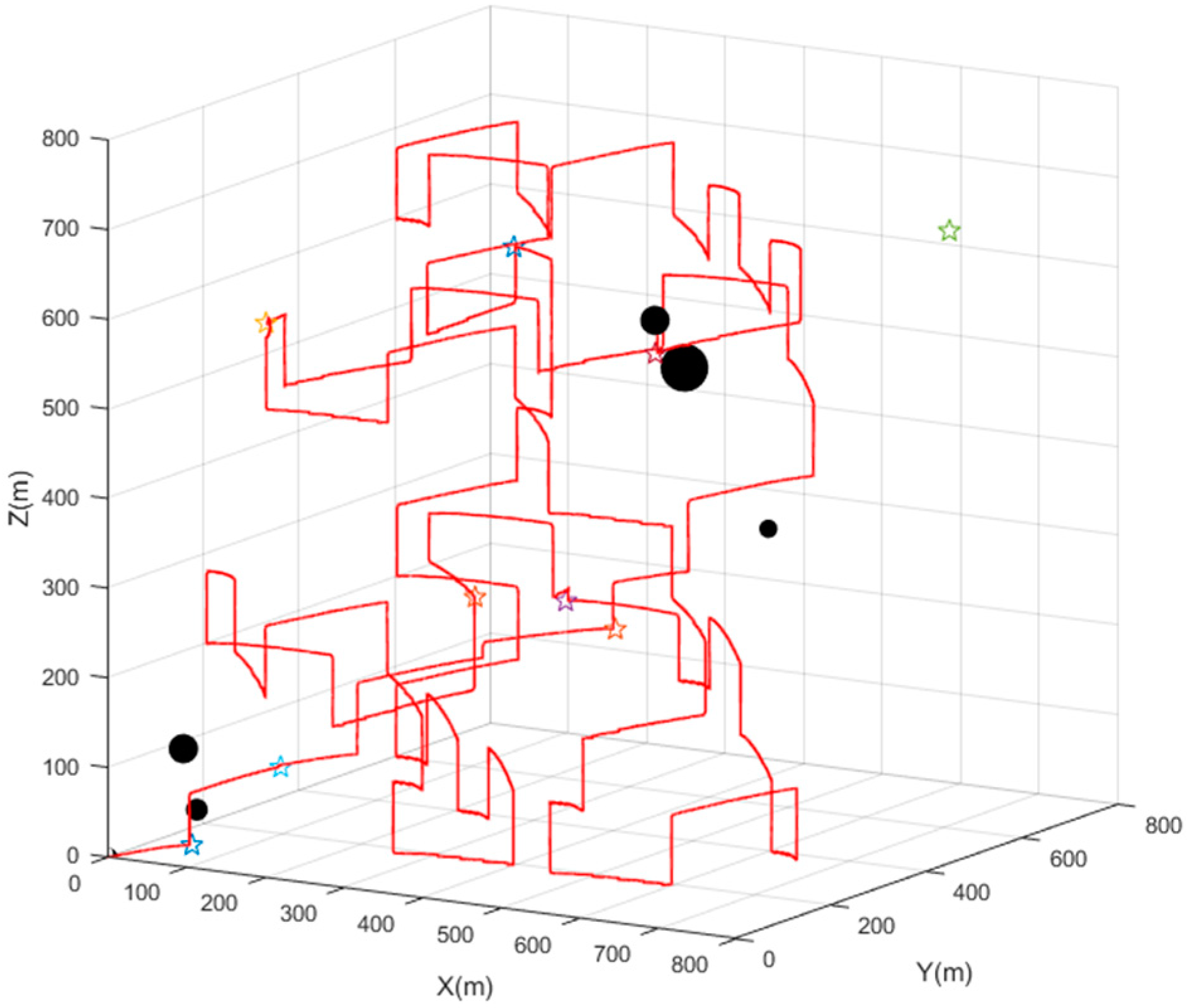
The AUV uses a target search algorithm based on the perception map to continuously determine the search location decision, and approaches the suspected target point when a suspected target appears within the sonar detection range until all the targets are searched. The final search trajectory diagram is shown in Figure 12.

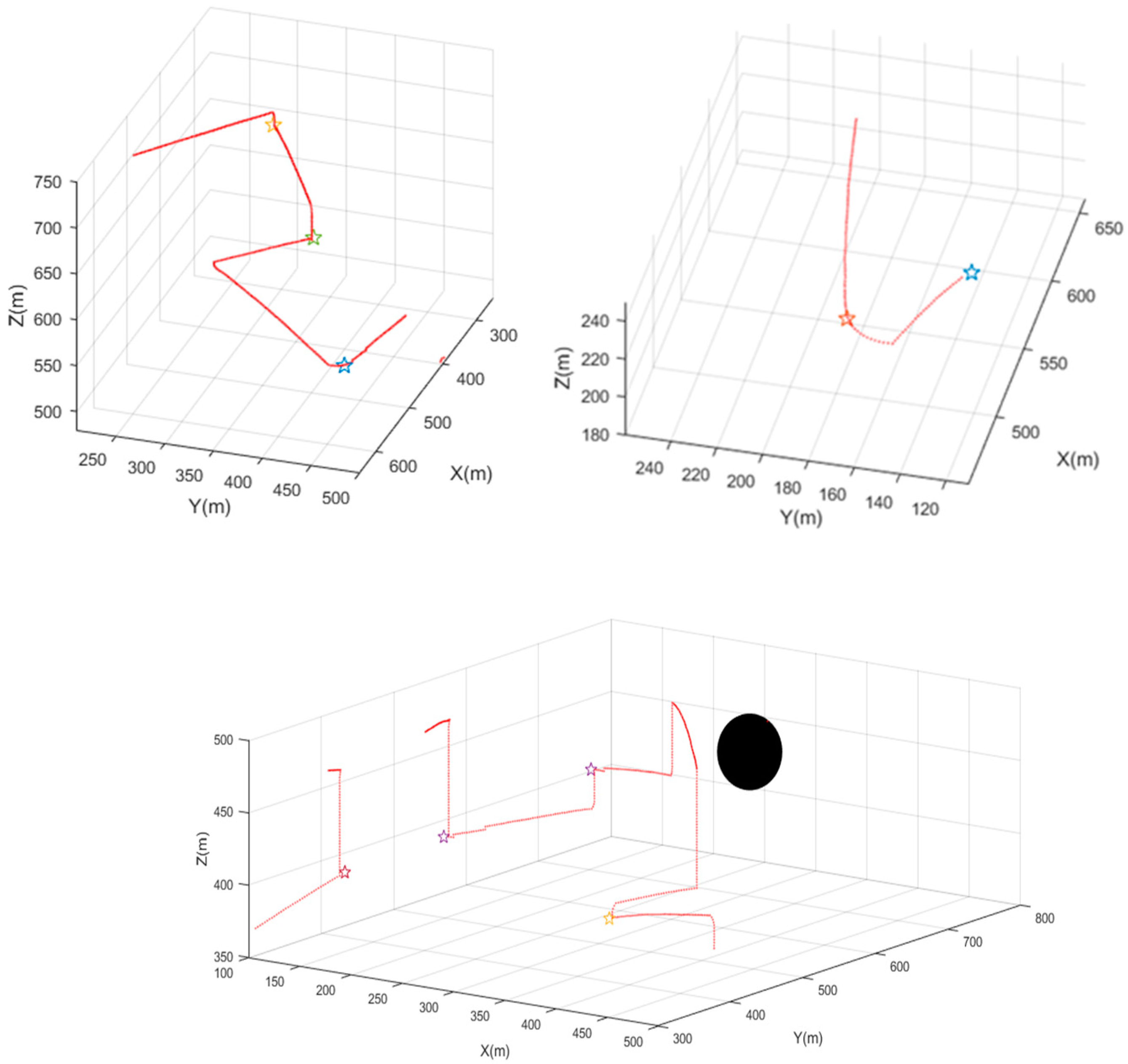
In order to avoid visual impact, the parts of search trajectories near (409.09,370.51,600.57), (476.40,169.42,283.27), (169.61,334.14,411.44) and other parts are locally amplified from different angles, such as in Figure 13. It proves the rationality of the target search algorithm described in this paper. This aspect will not be repeated in the following section.

7.2. Comparison and Simulation of Complete Coverage Search Algorithm

This section involves the same search environment as that in Section 7.1, and the AUV searches by the coverage search algorithm. By comparing the number of steps used by the AUV to search for all targets, the search efficiency of each algorithm is analyzed, and the efficiency of the target search algorithm proposed in this article is verified.

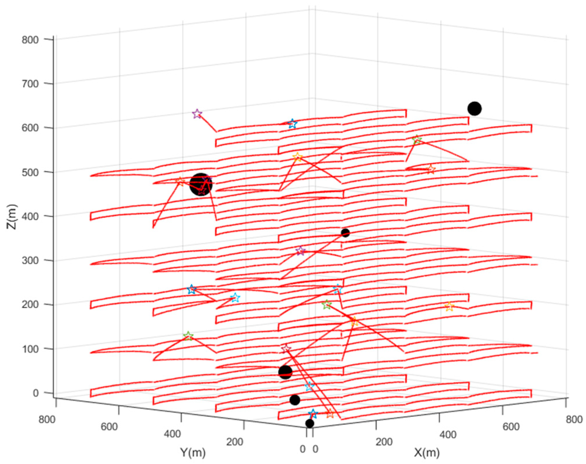
As shown in Figure 14, the AUV starts from the starting point (0,0,0), and searches hierarchically from bottom to top according to the traditional full coverage search method. The distance between each layer is 100 m. Additionally, when a suspected target point is found in the sonar detection range of the AUV, the AUV will go to the vicinity of the suspected target point for confirmation, and then return to the search position point planned by the previous coverage search algorithm until all the targets are searched. 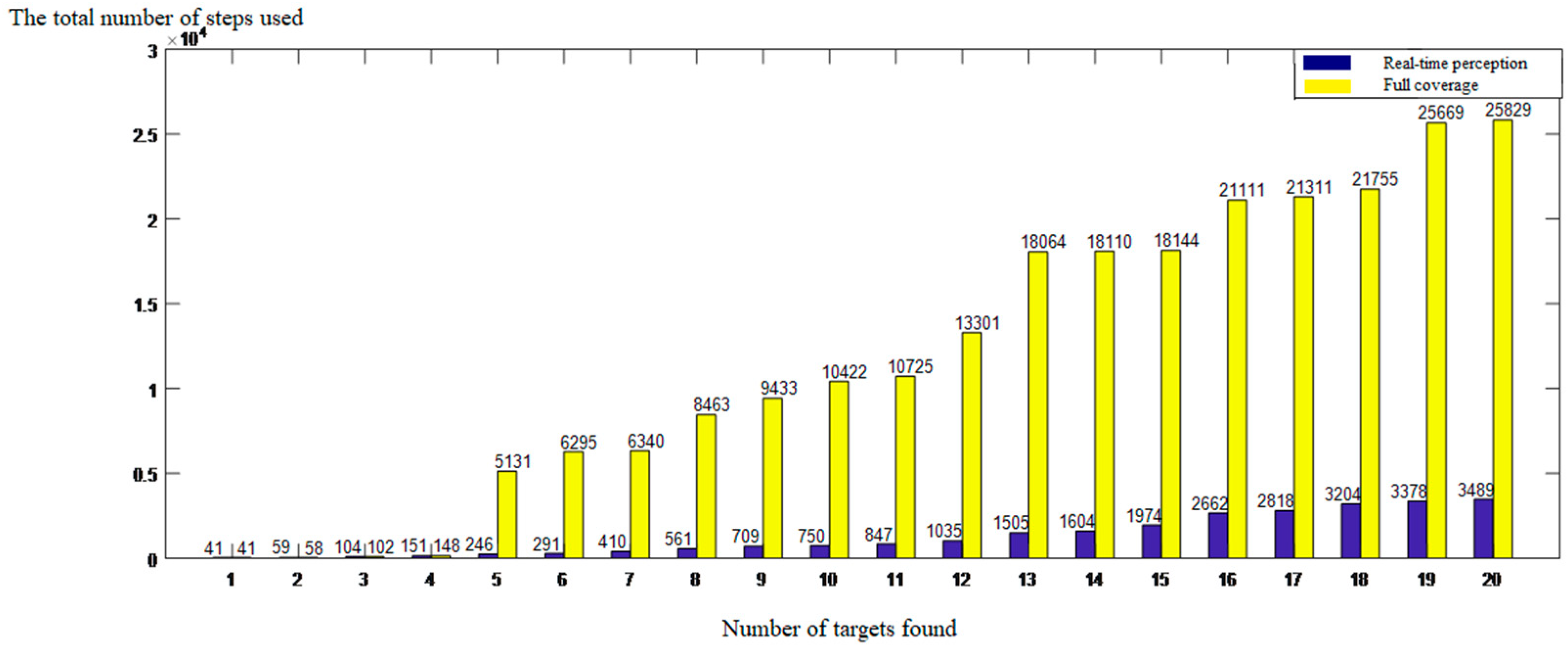Figure 15 shows the number of steps used by the AUV unknown target search algorithm and coverage algorithm described in this section to find each target.

In this section, ten random target point search comparison experiments are described, and 15 targets are randomly generated each time. The number of steps of the method in this study and the full coverage method after searching all targets is shown in

Table 3. Comparison of the number of steps used to search for all targets.

Number of Experiments	Target Search Algorithm in This Section	Full Coverage Algorithm
1	4963	29,065
2	2470	25,805
3	8414	29,040
4	3543	25,723
5	4480	24,289
6	3234	24,188
7	5806	28,989
8	4417	24,595
9	3063	24,272
10	2878	28,701

.

The analysis of Table 3 and Figure 15 shows that the complete coverage algorithm is robust, but it uses more steps to search for the target. It is shown that the AUV unknown target search algorithm proposed in this section uses fewer steps and improves search efficiency.

7.3. Comparative Simulation Experiment of Attraction Source

In order to test the effect of the attraction source on target search efficiency, two groups of comparative experiments are carried out in the same simulation environment. In the experiment in this section, the initial coordinate of the AUV is (0,0,0), and the coordinate of the target point is shown in

Table 4. Target point coordinates.

Target	Target Coordinates
Tar1	(70,60,10)
Tar2	(434,349,238)
Tar3	(110,150,580)
Tar4	(200,630,190)
Tar5	(680,645,655)
Tar6	(120,164,83)
Tar7	(600,160,600)
Tar8	(200,440,230)
Tar9	(140,620,580)

. The remaining parameter settings are the same as those in Section 7.1.

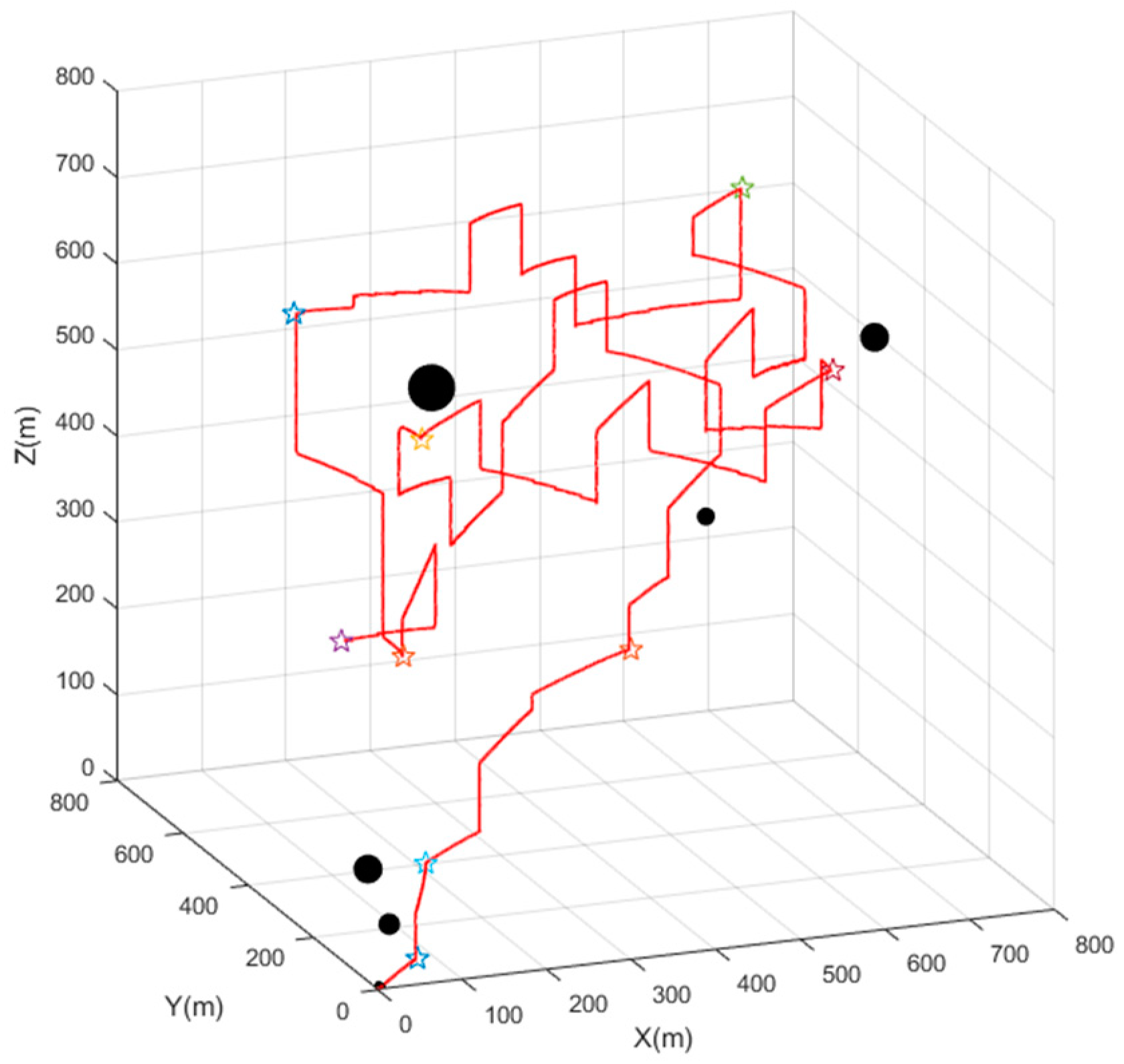
Experiment 1: Set up the attraction element

As shown Figure 16, in the early stage of the search with low search coverage, the AUV searches the central area according to the search gain formula, rapidly reducing the overall uncertainty of the environment. In the middle of the search, the weight of each gain in the search gain function changes, and the AUV is attracted by the activated attraction sources in the corner area. Therefore, the AUV searches corner areas with low coverage, and quickly finds the target points (680,645,655) and target points (140,620,580) at the corners. Then, the AUV searches for the target points (200,630,190) and (200,440,230) in the process of going to the activated attraction source in the lower left corner, and completes the search task.

Experiment 2: No attraction element is set up

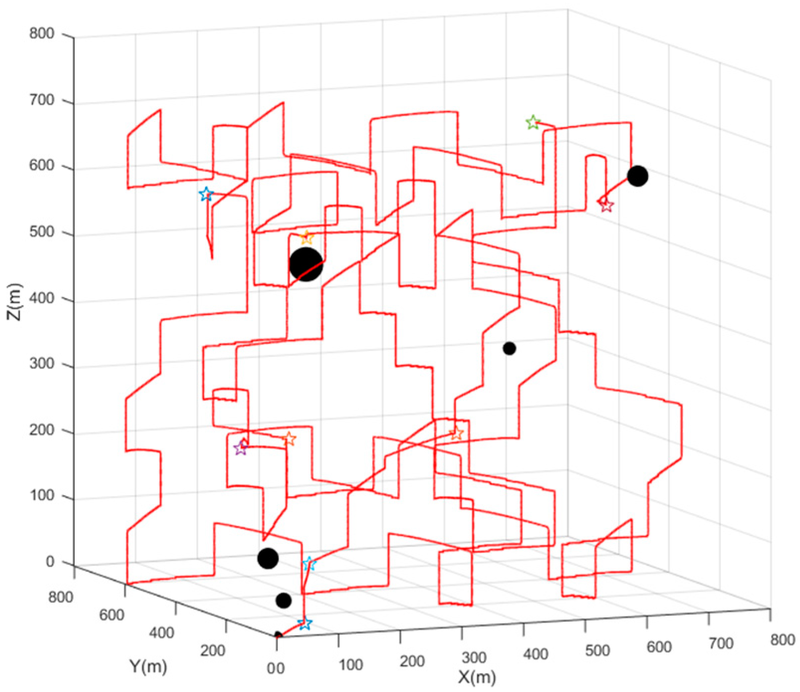
As shown in Figure 17, in the early stage of the search, in order to reduce the uncertainty of the entire search environment, the AUV searches more of the unsearched area in the center of the range, so the target point in the search center is searched faster. However, in the middle and late stages of the search, the AUV spends a lot of time searching areas with high coverage, and does not go to the corner areas with low search coverage where the target (680,645,655) is located.

As shown in Figure 18, when the AUV searches for the target point (600,160,600), the coverage of the corner area around the two points (600,600,200) and (600,600,600) is extremely low. Since there is no attraction source, the AUV only considers corner factors and other gains, and still moves towards the central area with higher overall search coverage.

For experiment one and experiment two, the number of steps used for each target is shown in

Table 5. Comparison of steps taken to find the target.

Tar	Experiment One	Experiment Two
Tar 1	42	41
Tar 2	123	123
Tar 3	345	346
Tar 4	1373	1235
Tar 5	1846	3037
Tar 6	2538	3375
Tar 7	3123	5345
Tar 8	3440	6769
Tar 9	3651	9857

. According to the experimental data, it can be seen that after setting the attraction source, the AUV searches for the target in the corner with less cost, and completes the unknown target search task with higher efficiency.

This section describes ten sets of comparison experiments with random target coordinates. By comparing the change in the total uncertainty of the search environment within 3600 steps of the target search algorithm with and without the attraction source, the influence of the attraction source is verified. The total uncertainty is calculated every 600 steps in ten experiments. The average data of ten experiments are shown in

Table 6. Comparison of steps taken to find the target.

Step Count	Added Source of Attraction	No Attraction Element
0	512	512
600	467.456	467.456
1200	426.458	426.458
1800	389.529	389.529
2400	341.693	347.223
3000	306.947	315.897
3600	274.044	287.273

.

Analyzing the data above, it can be seen that after the attraction source is set, the AUV will actively search the corner areas with low search coverage, and the corner targets are easier to find. Additionally, the overall uncertainty of the task area decreases faster in the middle of the search, thereby improving the target search efficiency of the algorithm.

8. Conclusions

This paper proposes an AUV target search algorithm based on a real-time perception map. The algorithm improves the target search efficiency of an AUV in an unknown underwater environment, and the following conclusions are drawn through simulation verification:

(1) The attraction source map activates the attraction source in the corner area to continuously release the attraction pheromone. Through the diffusion method of the neural excitation network, the attraction pheromone forms a gradient, which guides the AUV to search for corner areas that are unknown to a higher degree. However, the traditional search does not add a source of attraction, which makes the traditional search unable to search the corner area well, and will miss the target in the corner area. Even if the target in the corner area can be searched, the traditional method will waste a lot of time.

(2) The search status map guides the AUV to search the area with low coverage around the current location by dividing the search status of the grid.

(3) By considering the actual underwater search situation of the AUV, the update formulas of the target existence probability map and the revisit map have been improved to make the update of the real-time perception map more in line with the underwater search task.

(4) The artificial potential field method is improved by considering the rotation angle limit of the AUV and the volume of obstacles. The artificial potential field method is used to plan the path of the AUV. The AUV can reach the decision point with a shorter path, and it is in line with the actual navigation situation of the AUV.

(5) Through comparative experiments, the effectiveness and efficiency of the target search algorithm based on a real-time perception map is verified, and the efficiency improvement of the algorithm by an attraction source map is separately verified.

In this study, the variation in the sonar performance during the navigation has not been considered since the main purpose of this study is to reduce the uncertainty of the entire search environment by an AUV within the specified time frame. Therefore, the AUV target search algorithm proposed in this paper is weak in searching boundary discrete targets, and further research is needed.

The innovation of this article is mainly to adopt a variety of search strategies and attraction source maps. According to the different times of the AUV search process, different search strategies are adopted, which can quickly reduce the unknown degree of the environment and the target search time. An AUV can increase the feasibility of searching corner areas according to the attraction source map, which is conducive to the search of the corner areas. However, the algorithm in this study cannot effectively reduce the time when there are too many search targets concentrated in the corner areas or there are dynamic obstacles in the environment