Abstract
In this paper, a complete set of nonlinear modeling and controller design process for a small electric fixed-wing unmanned aerial vehicle (UAV) is presented. The nonlinear mathematical model and aerodynamic model of the small fixed-wing UAV are derived. The computational fluid dynamics (CFD) method was used to obtain the aerodynamic coefficients of the UAV, and the models of propulsion system components were established through experiments. Since the linearized and decoupled model of the fixed-wing UAV has a large error, a nonlinear model is established based on Simulink, which is utilized to design and verify the control algorithms. Based on the established nonlinear model, a stability controller, path following controller and path management controller of the aircraft are set up. The results indicate that system parameters of the aircraft can be quickly acquired and an efficient and practical model can be established by the methods. In addition, the controller designed and applied in this paper has good performance and small steady-state error, which can meet the basic flight mission requirements, including stability of flight attitude, path following and switching of different waypoints. These modeling and control methods can also be employed in other small battery-powered fixed-wing UAV projects.
1. Introduction
UAVs have attracted increasing research attention in the last decades and gained many applications in both civilian and military operations with improvements in avionics devices. The UAVs have been employed for agricultural monitoring, reconnaissance, photography and remote sensing [1,2,3,4]. Due to the convenience and high flexibility of small UAVs, the demand for their development and application continues to increase.
Small UAVs refer to UAVs weighing less than 5 kg, including small fixed-wing aircraft, helicopters and multicopters [5]. UAVs are mostly powered by battery, and a few UAVs are powered by fuel [6]. Compared with rotary-wing UAVs, fixed-wing UAVs have longer endurance and better flight efficiency [7]. The aerodynamic layout of a fixed-wing aircraft can affect its lift-to-drag ratio, which in turn affects endurance [8]. Flying wing UAV is a non-canard and tailless aircraft with integrated fuselage and wing [9]. The unconventional aircraft has lower aerodynamic drag compared with the conventional configuration, while the special aerodynamic shape will add more challenges to the stability of the aircraft [10,11]. In order to develop a small electric UAV with flying wing configuration, it is vital to measure the system parameters, establish an accurate mathematical model and design a reliable controller.
Predicting aerodynamic forces and moments of the UAV is very difficult due to the external disturbances [12] and there are several approaches utilized to assess the aerodynamic derivatives and characteristics of the fixed-wing UAV. Wind tunnel testing [13], DATCOM software [14], empirical relations [15], flight testing [16] and CFD simulation [17] are employed to acquire aerodynamic characteristics of the UAVs in different studies. Wind tunnel testing is one of the most important tools because it can accurately control the environmental conditions and the measurement results are accurate; however, its equipment is expensive and the tests are complex. Flight testing is easily affected by external disturbances. The results obtained by DATCOM software and empirical relations usually have more errors than other methods. CFD method may not obtain accurate results, and the simulation results will be affected by parameters such as grid quality and boundary settings; however, it is very suitable for the preliminary design of aircraft.
For a small electric fixed-wing UAV, in addition to the aerodynamic coefficients, it is also important to obtain the parameters of the propulsion system. The thrust and torque data of a small UAV’s propulsion system can be obtained by wind tunnel tests [18]. ZHAO proposed a novel airborne test method suitable for fixed-wing aircraft, which can replace the high-cost wind tunnel test [19]. Piljek proposed a method for characterization of the multirotor UAV propulsion system, and conducted experimental measurements to validate the method [20]. Virginio proposed a low-cost Thrust Benchmarking System for an electric UAV propulsion system, and three kinds of propellers were modeled by the instrument [21]; however, the propulsion system and actuator models required for UAV modeling have not been well summarized.
Since the fixed-wing UAV is a nonlinear and strongly coupled system, linearization of equations of motion using small perturbation theory is often used in literature. UAV equations of motion can be separated into longitudinal and lateral directional dynamics and decoupled between them. The perturbation with little difference from the reference motion is called the small perturbation motion. Such difference is related to the specific situation and has no absolute value. This assumption is no longer applicable to a UAV that needs to complete multiple flight missions, such as hovering and landing. A mini-UAV designed for agricultural application was separated into longitudinal and lateral state-space models, and five different controllers were designed for the UAV lateral dynamics [22]. An MPC strategy based on the lateral and longitudinal linear models was proposed to examine a fixed-wing UAV as it undergoes five flight scenarios [23]. Melkou adopted an uncertain linear model decoupled into longitudinal and lateral directional modes to represent the aircraft and added a PID outer loop to improve the accuracy [24]. The method of linearizing and decoupling a fixed-wing UAV is very common, and it is convenient for researchers to design controllers; however, the linearized model will produce larger errors in the process of simulation and flight test, and the use of nonlinear models can better predict the aerodynamics of the UAV [25].
The previous studies indicate the importance of small electric UAVs and how difficult it is to design and develop them. For aircraft conceptual design, there are some methodologies [11,26]. A methodology for sizing the electric propulsion subsystems of UAVs was developed by Gokcin [27]. Avanzini proposed a methodology to obtain best-endurance and best-range conditions by optimizing the aircraft size [28]; however, there are few studies on flying wing configuration UAVs with only two elevons, and most of the design and research on fixed-wing UAVs are based on linearized models. This work focuses on the mathematical modeling and controller design of the unconventional UAV configuration. The methodologies to acquire the parameters of the UAV system, including parameters of the aerodynamic structure and electric equipment, are well summarized, and the nonlinear model of the small electric flying wing UAV is quickly established. The stability controller of the UAV is established based on PID algorithm by combining the characteristics of the small electric flying wing UAV. The shortcomings of some previous path-following methods are summarized in this paper, and a comprehensive and optimized path-following algorithm is proposed. As an initial stage in this work, the nonlinear mathematical model, including the 6-DoF equations of motion and aerodynamic model, is derived. Aerodynamic derivatives are obtained using the CFD software Fluent and propulsion system parameters are acquired by corresponding tests. A complete, efficient and practical simulation model was quickly established to verify the effectiveness of the algorithm. In the final stage of the work, a stability controller, path following controller and path management controller were designed and verified in turn. A set of systematic development procedures of a small electric fixed-wing UAV is presented in this paper, which provides a reference for the design and development of other small electric fixed-wing UAVs. MATLAB/Simulink was utilized to establish the mathematical model, solve the nonlinear equations of motion numerically and validate the control method in our research. The remaining part of the paper is organized as follows. In Section 2, the nonlinear mathematical modeling of the fixed-wing UAV is indicated. In Section 3, we detail the parameters of the UAV system obtained by experiments and simulations. The controllers, including the stability controller and the upper controllers, are explained in Section 4. Discussion on system parameters measurements and control methods is presented in Section 5. Finally, the summary and conclusions are presented in Section 6.
2. Mathematical Model of the Fixed Wing UAV
The geometry model and aerodynamic shape data of the UAV investigated in our study are taken from our previous work [29], which is shown in Figure 1. The geometrical values are given in Table 1. In Table 1, AR is the aspect ratio, S is the area of the wing, b is the wingspan, c is the mean aerodynamic chord of the wing and ma is the mass of the UAV. The small fixed-wing UAV we designed only has two control surfaces, as known as elevon, and they have the same effects as both ailerons and elevators, and it has a brushless DC electric motor at the end side of the UAV to provide thrust. Based on this aerodynamic shape, we made a prototype for accurate parameter identification, but there are some differences with theoretical parameters. For example, the theoretical gross weight is 1.5 kg, but the actual mass is 0.9 kg.
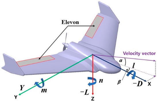
Figure 1.
Small battery-powered flying wing UAV.

Table 1.
Numerical values of the UAV.
2.1. 6-DOF Equations of Motion
In order to design and validate the UAV control system, it is very important to describe the details of the UAV’s dynamics and kinematics. The six degrees of freedom nonlinear model of the UAV consists of force equations, moment equations and kinematic equations for position and navigation. These dynamic equations for the UAV are given as follows [30].
Force equation:
where Vb = [u, v, w] are velocities of the UAV in the x, y and z body axis, while ω = [p, q, r] are the angular velocities about the same axis, respectively. Fb is the sum of all the forces acting on the UAV in the body axis.
Moment equation:
In Equation (2), Ib is the 3 × 3 inertia matrix of the UAV and Mb is the sum of external moments of the body axis.
Position equation:
where pe represents the position of the UAV in the Earth coordinate system; is transformation matrix from body axis to Earth axis. Navigation equation:
where Θ = [φ, θ, ψ] are Euler angles, W is transformation matrix from angular velocities to Euler rates. When the initial conditions of the UAV are determined, the attitude and position information of the UAV can be obtained by inputting the force and the moment into the system. For the UAV, the force can be split into thrust Ft, gravity Fg and aerodynamics forces Fa, as seen in Equation (5). Since the gyroscopic moment generated by the rotation of the propeller and the motor is far less than other moments, it is approximately zero here. Similarly, the moment on the UAV, which is assumed to act around the center of gravity, can be decomposed into the counter torque Mt exerted by the propeller [31] and the aerodynamic moments Ma, as seen in Equation (6).
Fb = Ft + Fg + Fa
Mb = Mt + Ma
The thrust and the counter torque generated by the rotating propeller were obtained through experiments, detailed in subsequent sections. The aerodynamic moments are modeled in the body frame, but the aerodynamic forces are modeled in the wind frame, which need to transform to the body frame, as seen in Equation (7).
where Fx, Fy and Fz indicate the aerodynamic forces along x, y, z axis of the body frame; D, Y and L denote the aerodynamic drag force, side force and lift force acting along the negative x, positive y and negative z wind axis, respectively, is transformation matrix from wind axis to body axis. More details about the modeling of the UAV are shown in (A1)–(A3).
2.2. Aerodynamic Model
Since UAVs have different aerodynamic characteristics under different conditions, modeling the aerodynamic forces and moment is one of the most vital and complicated parts of designing a fixed-wing UAV. A commonly used model for aerodynamic forces and moments acting on a fixed-wing UAV is shown in Equations (8) and (9).
where ρ is the air density, Va is the airspeed of the UAV. CD, CY and CL are the non-dimensional coefficients of drag, side and lift force, respectively. l, m and n denote the aerodynamic moments along x, y and z-axis of the body frame and can be modeled in terms of the dimensionless functions Cl, Cm and Cn, respectively. All the aerodynamic forces are modeled in the wind frame.
The aerodynamic coefficients of forces and moments depend on many variables with complicated nonlinear correlation, and it is a mathematically convenient way to build up the coefficients as a sum of contributing components. There are several kinds of expressions for the force and moment coefficients, and a simple but reasonable expression [32] is employed in this paper, as seen in Equations (10) and (11).
where α is the angle of attack and β is the sideslip angle, δe, δa, δr denote the elevator, aileron and rudder deflection of the UAV, respectively. Due to the particular structure of the flying wing UAV, δr is set to 0, δe and δa can be decoupled into expressions of left and right elevon deflections by Equation (12). All the other aerodynamic coefficients are presented in the following section and their values are given in Table 2.
Table 2.
Aerodynamic coefficients of the UAV.
δer and δel represent the angular deflections of the right and left elevon, respectively—assuming that the aerodynamic effects of the left and right elevons are the same and there is no coupling between them. In Section 3, the aerodynamic coefficient values affected by δe and δa are obtained, which are twice the values affected by a single elevon. So aerodynamic forces and moments can be calculated with coefficients of δer and δel.
3. System Parameters Measurements
For establishing an accurate nonlinear simulation model of the UAV, some system parameters need to be measured to improve the UAV model, including aerodynamic derivatives, propulsion system parameters and basic parameters of the UAV. All the simulation and test data are fitted through the curve fitting toolbox in MATLAB, and the fitting results are presented in the following subsections.
3.1. Aerodynamic Derivatives Measurements
All the aerodynamic derivatives can be divided into static stability derivatives (influenced by α and β), damping derivatives (influenced by p, q, r) and control derivatives (influenced by δe and δa) and their values determine the static stability, dynamic stability and control effects of the UAV, respectively. CFD method is investigated and used in this paper to obtain the aerodynamic characteristics of the UAV numerically through comprehensive consideration of accuracy and convenience.
The stability derivatives and the control derivatives can be obtained under steady-state simulation conditions, while the damping derivatives need dynamic simulation conditions. In this work, the stability derivatives and the control derivatives are collectively referred to as static derivatives, and the damping derivatives are referred to as dynamic derivatives. The aerodynamic analysis of the UAV and the calculation of all the aerodynamic derivatives were implemented with the Fluent software. The finite volume method is employed to solve the N-S equations to acquire aerodynamics [33], and the SST k-w turbulence model is utilized as the fluid model.
3.1.1. Static Derivatives
In the simulation of calculating the static derivatives, the air velocity is set to 15 m/s. The tests focus on the quality of the model around α = β = δe = δa = 0. The corresponding changes of aerodynamic coefficients can be obtained by changing the values of the parameters. The Reynold number for the UAV corresponding to cruise speed is about 400,000 when the air temperature is 288.15 K and the air density is 1.225 kg/m3.
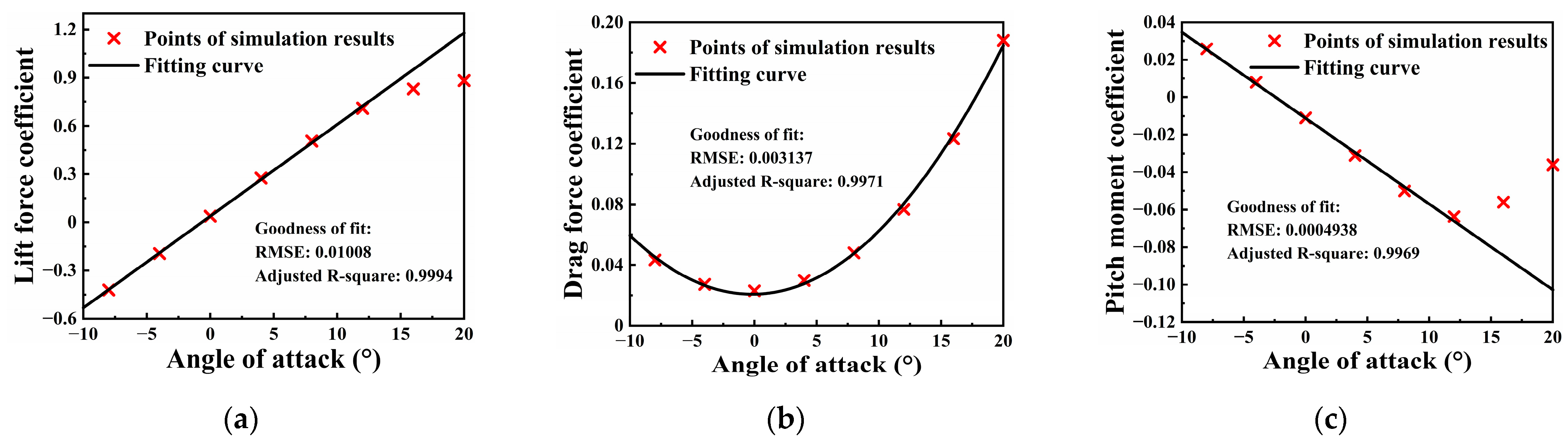
In Figure 2, the lift force coefficient, drag force coefficient and pitch moment coefficient are presented as a function of the angle of attack. When the angle of attack is −10° to 12°, the lift force coefficient and pitch moment coefficient increase linearly. The airflow begins to separate and the nonlinear phenomena of the lift force and the pitch moment occur when the attack angle exceeds 12°. The UAV is close to the stall at 20° angle of attack. In this study, in order to facilitate modeling, they are approximated as linear models. Since the UAV designed in this paper rarely has a high attack angle during flight missions, the error caused by linearization is tolerable; however, the linearized model may not be applicable to complex missions that require a high attack angle. It should be noted that only the data with an attack angle less than 16° is used for the fitting of the lift and pitch moment coefficients. This is to make the model more accurate with a small attack angle. As shown in Figure 2b, the drag force coefficient curve can be well fitted with a quadratic curve.
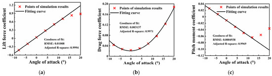
Figure 2.
Curve fitting of aerodynamic coefficients versus the angle of attack: (a) lift force; (b) drag force; (c) pitch moment.
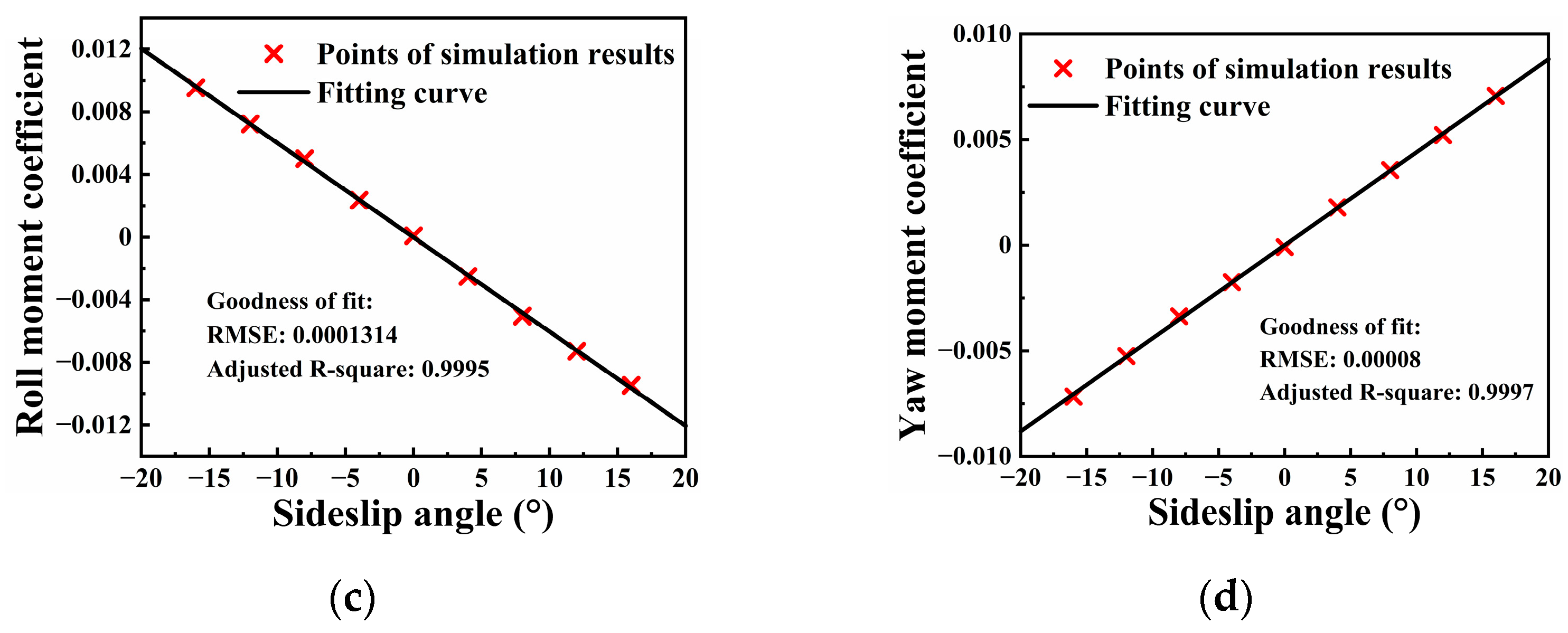
The sideslip angle is one of the parameters that have the greatest impact on the UAV due to external wind interference, and it can affect a number of aerodynamic parameters of the fixed-wing UAV, which we can see in Figure 3. The drag force, side force, roll moment and yaw moment coefficients are plotted versus the sideslip angle in Figure 3. In the range of sideslip angle of −20° to 20°, the drag force coefficient uses quadratic fitting, and the other coefficients use linear fitting.
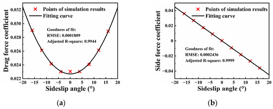

Figure 3.
Curve fitting of aerodynamic coefficients versus the sideslip angle: (a) drag force; (b) side force; (c) roll moment; (d) yaw moment.
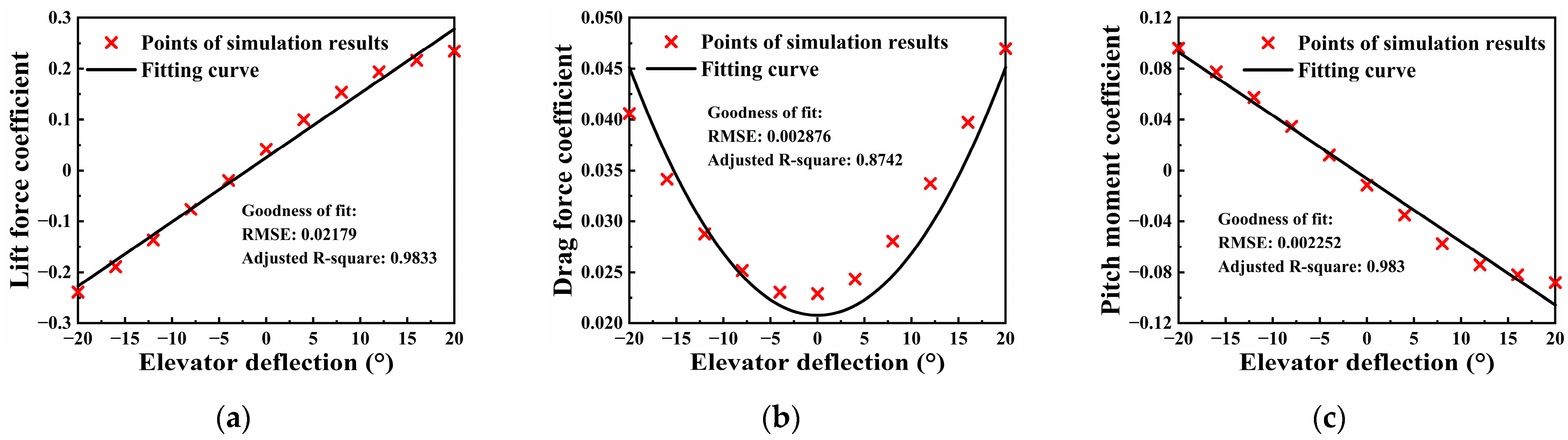
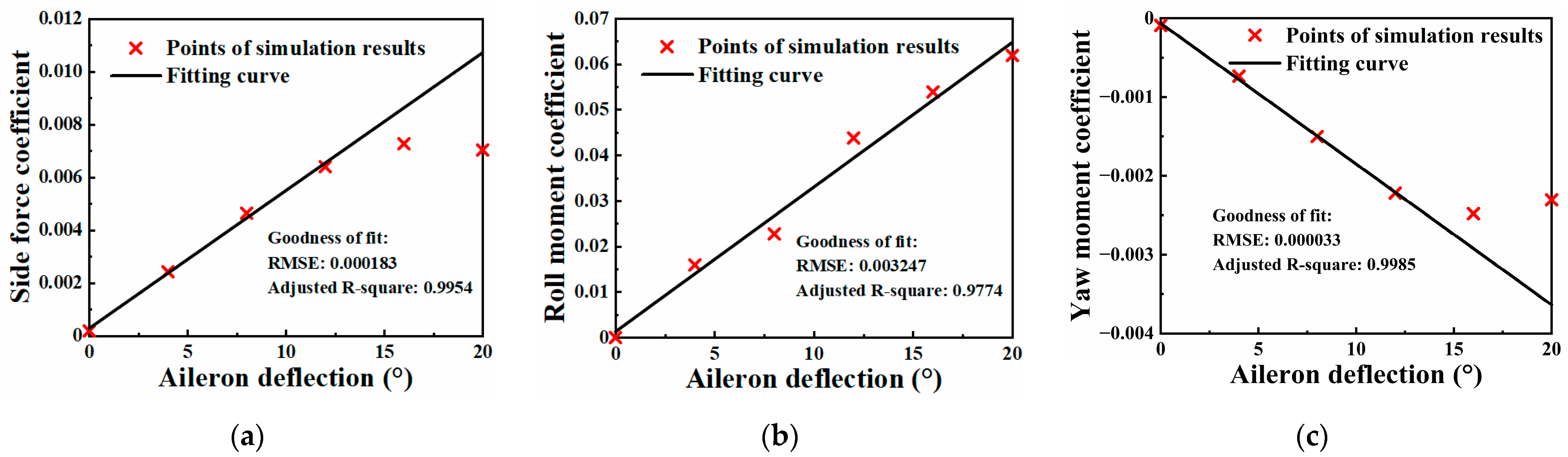
In Figure 4 and Figure 5, the aerodynamic force and moment coefficients are plotted as functions of the elevator deflection and the aileron deflection. The values of the control derivatives are equal to the slopes of these curves. As shown in Figure 4, the lift coefficient and pitching moment coefficient increase linearly with the increase in the elevator angle. Due to the asymmetric shape of the elevator’s upper deflection and lower deflection, the drag coefficient is not completely symmetric on both sides of δe = 0°. For the convenience of modeling, we only keep the quadratic term of the curve, which will result in a maximum error of 12% when δe = 12°. Such error introduced by the hypothesis of keeping the drag symmetric is within the acceptable range, so we ignore it here. Due to the symmetrical shape of the UAV, it is only necessary to calculate the aileron angle of 0° to 20° to reduce the simulation time. As shown in Figure 5, when the aileron angle is below 16°, with the increase in the aileron angle, the side force coefficient and roll moment coefficient increase approximately linearly, and the yaw moment coefficient decreases linearly. Since the aileron has little effect on the side force coefficient and the yaw moment coefficient, they are approximated as a linear relationship to simplify the model. For the same reason as the attack angle, the fitting curve does not include the data of side force and yaw moment coefficients when δa is 16° and 20°.
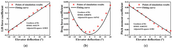
Figure 4.
Curve fitting of aerodynamic coefficients versus the elevator deflection: (a) lift force; (b) drag force; (c) pitch moment.
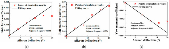
Figure 5.
Curve fitting of aerodynamic coefficients versus the aileron deflection: (a) side force; (b) roll moment; (c) yaw moment.
3.1.2. Dynamic Derivatives
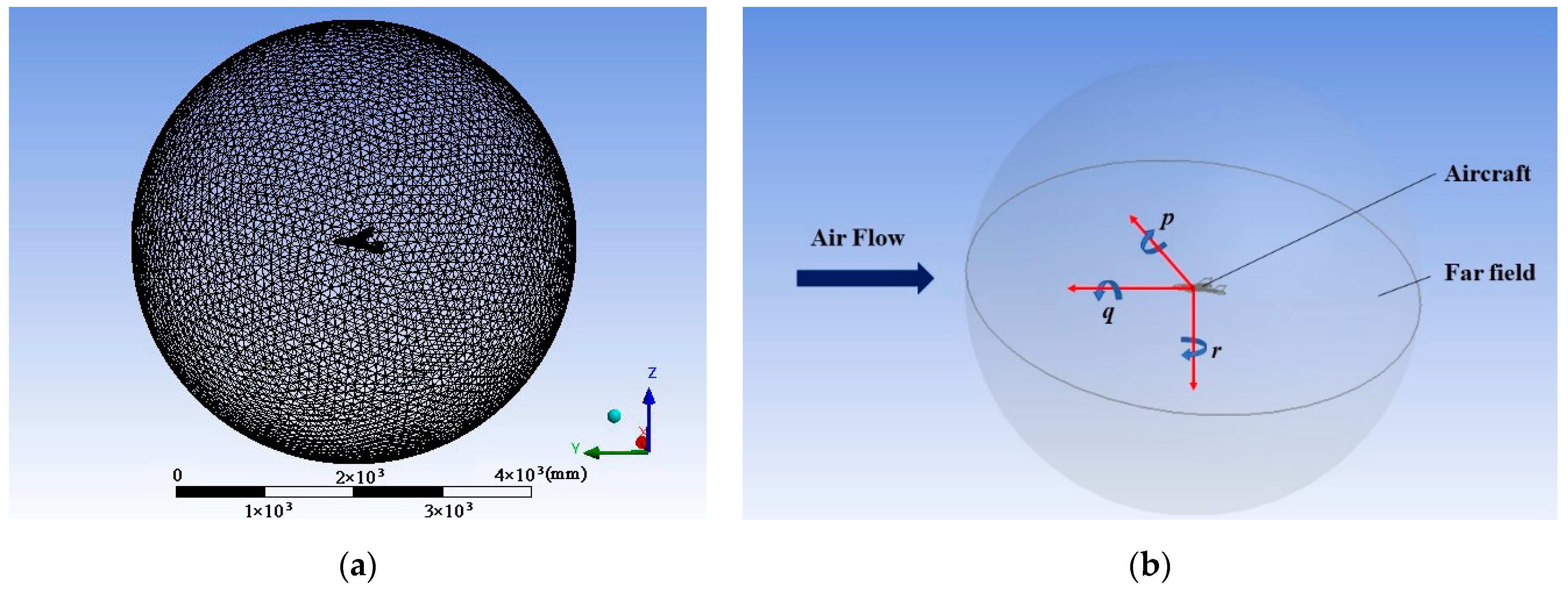
In addition to the settings of calculating static coefficients, the rotating reference frame is adopted to gain the dynamic derivatives by simulation of the steady movement [34]. The unsteady flow field required for aircraft simulation can be converted into a steady flow field by the rotating reference frame method. The SRF (Single Reference Frame) model is utilized to simulate the rotation with the constant angular velocity of the UAV about the x, y, z-axis of the body frame in Fluent software, respectively. Boundary settings and meshes of the far-field are shown in Figure 6. An unstructured mesh is used to save computing time. The first height of the boundary layer mesh is 2 × 10⁻⁵ m and y+ is 1. The growth ratio is 1.2 and 10 boundary layers are generated. The total number of 3D computational grid is about 4 × 10⁶. As shown in Figure 6b, velocity-inlet with magnitude and direction is selected in the far-field, which can ensure the airflow flows vertically to the aircraft when the fluid domain rotates. The unit of angular velocity is expressed in terms of rad/s in this subsection.
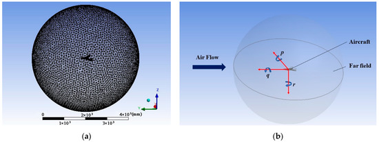
Figure 6.
Grids for far-field and boundary conditions. (a) Meshes of the fluid domain; (b) boundary conditions.
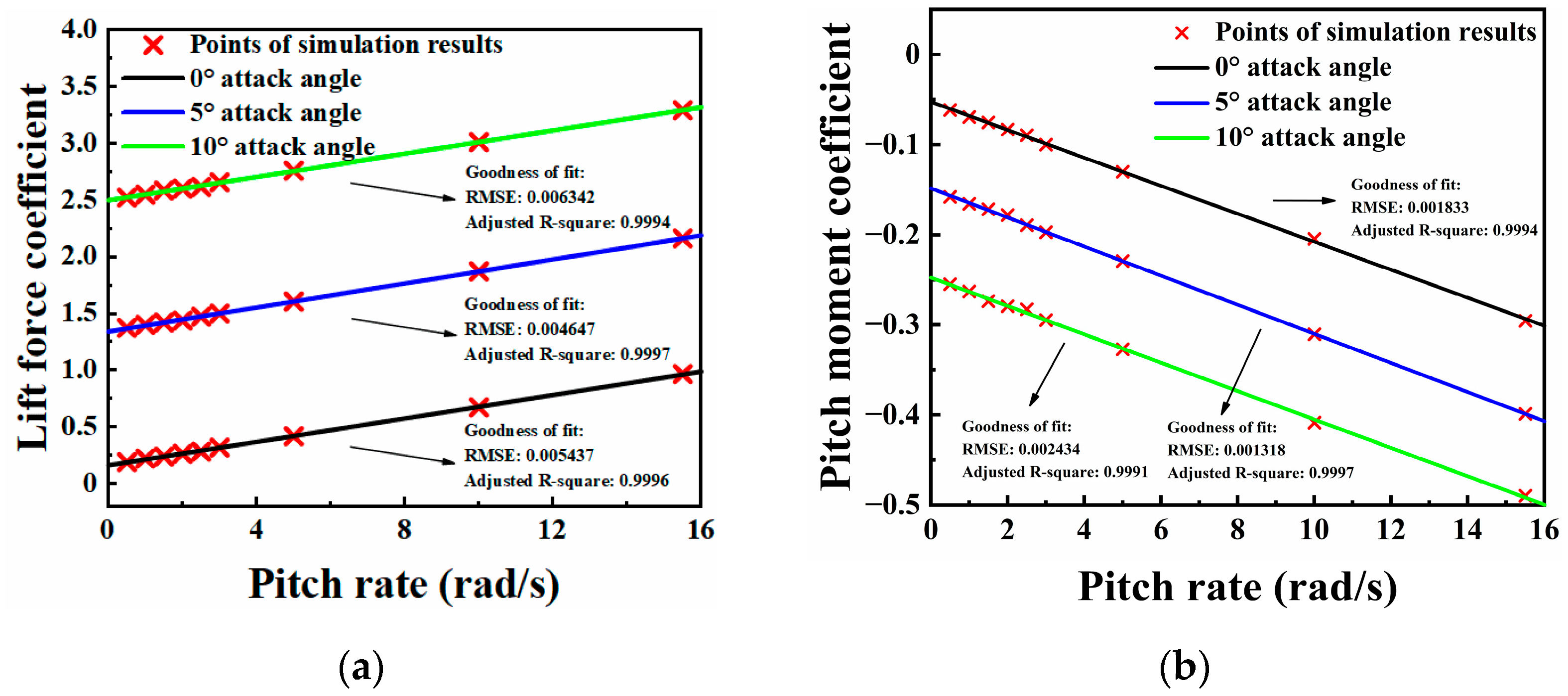
In Figure 7, the lift force and pitch moment coefficients are presented as functions of the pitch rate for various attack angles. Since the fluid domain needs to simulate the steady climb movement of the UAV when obtaining aerodynamic coefficients related to pitch rate, only positive rate values are considered. The lift force coefficient and pitch moment coefficient increase linearly, with pitch rate increasing at different attack angles. In this study, because the slope of the drag force coefficient curve is approximately zero, the influence of the pitch rate on the drag force is ignored.
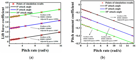
Figure 7.
Curve fittings of lift force and pitch moment coefficients versus the pitch rate at various attack angles: (a) lift force; (b) pitch moment.
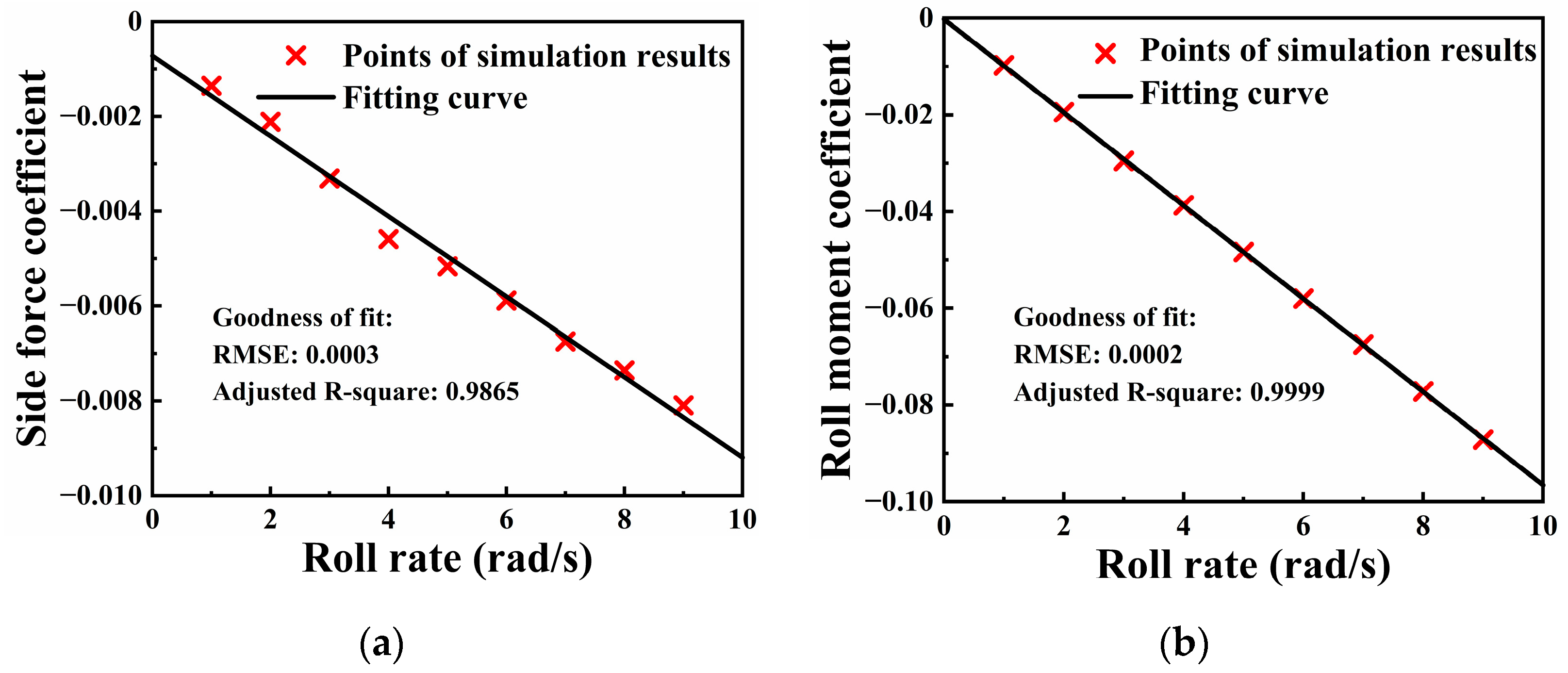
The side force and roll moment coefficients versus the roll rate are plotted in Figure 8. The side force and roll moment coefficients decrease linearly with the increase in the roll rate. In this study, the roll rate has little effect on the yaw moment coefficient, so it is ignored here.
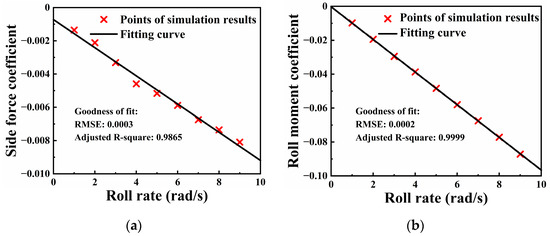
Figure 8.
Curve fitting of aerodynamic coefficients versus the roll rate: (a) side force; (b) roll moment.
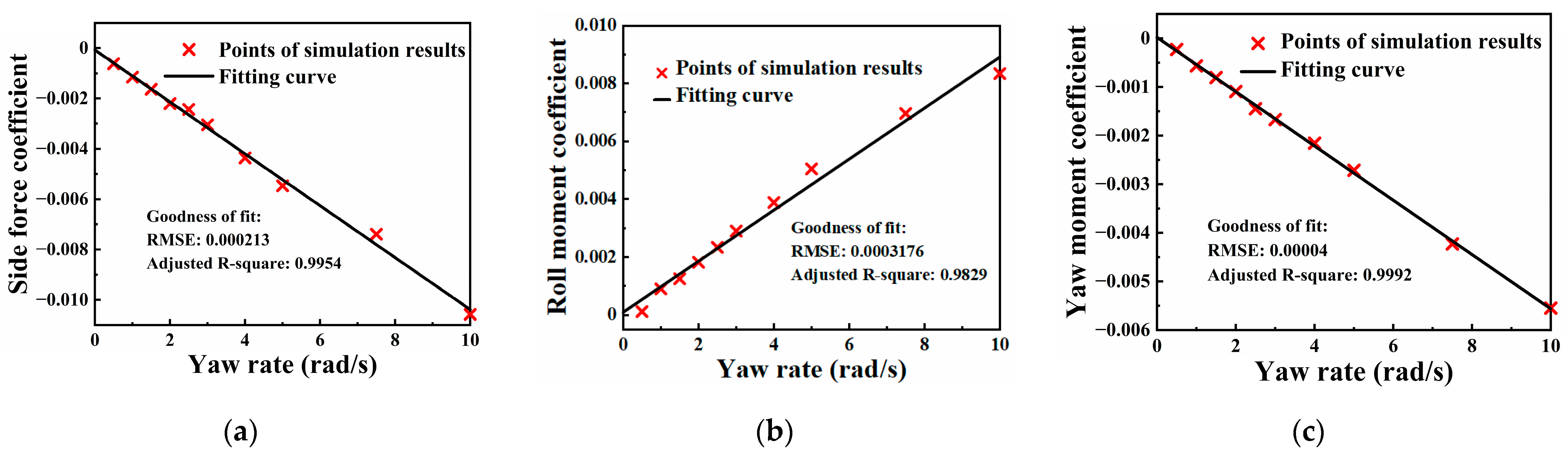
The side force, roll moment and yaw moment coefficients versus yaw rate are presented in Figure 9. With the increase in yaw rate, the side force coefficient and yaw moment coefficient decrease linearly, while the roll moment coefficient increases linearly.
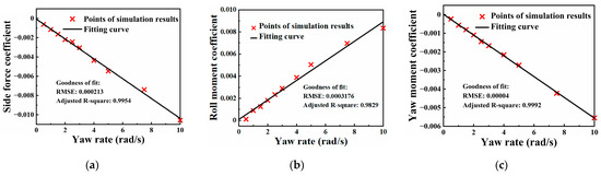
Figure 9.
Curve fitting of aerodynamic coefficients versus the yaw rate: (a) side force; (b) roll moment; (c) Yaw moment.
All the values of the aerodynamic derivatives calculated from Fluent software and the results with 95% confidence bounds fitted by MATLAB are summarized in Table 2. Angles and control surface deflections are given in radians, and angular rates are expressed in terms of radians per second when calculating the aerodynamic derivatives. Among these coefficients, Cmα < 0, Cnβ >0 and Clβ < 0 indicates the UAV has a longitudinal, yaw and lateral static stability.
3.2. Propulsion System Measurements
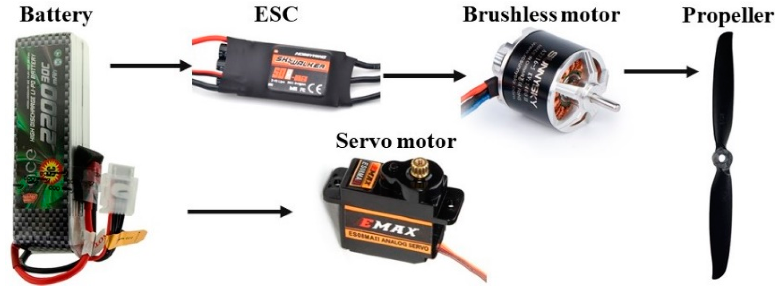
The propulsion system components consist of a propeller, brushless DC (Direct Current) motor, Li-Po (Lithium Polymer) battery and ESC (Electronic Speed Control) unit. In addition to the propulsion system components, the actuator of the elevon is also tested in this section, as shown in Figure 10. The propulsion system components were selected according to the structure, size and weight of the UAV investigated in this study. A SunnySky 2216 KV2400 electric brushless motor with a 6040 propeller and a Grepow 2200 mA·h 4S (16.8 V) Li-Po battery were adopted and tested in this research.

Figure 10.
Propulsion system components and the servo motor of the UAV.
3.2.1. Propeller Model
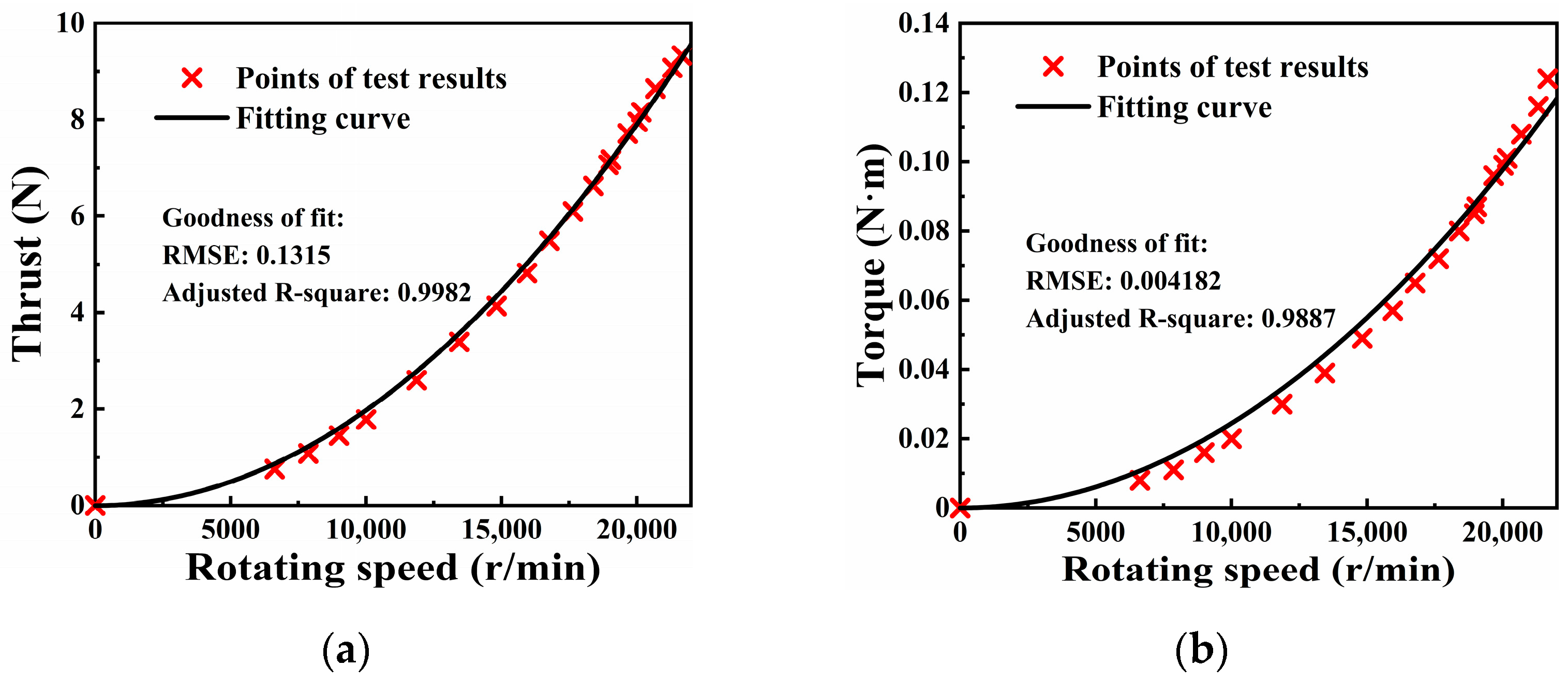
Generally, the thrust generated by the propeller during the flight of the UAV depends not only on the rotating speed of the propeller but also on the airspeed [35]. Since the airspeed of the UAV used in this study is relatively small, only the influence of the rotating speed on the thrust is considered to simplify the model. The thrust and the counter torque exerted by the propeller [36] can be obtained by Equation (13).
where Dp denotes the diameter of the propeller (m), CT and CM are dimensionless coefficients representing thrust and torque, N denotes the rotating speed (RPM). Since Dp and ρ are constants, T and M can be expressed as quadratic functions of N with coefficient KT and KM, respectively, as shown in Equation (14).
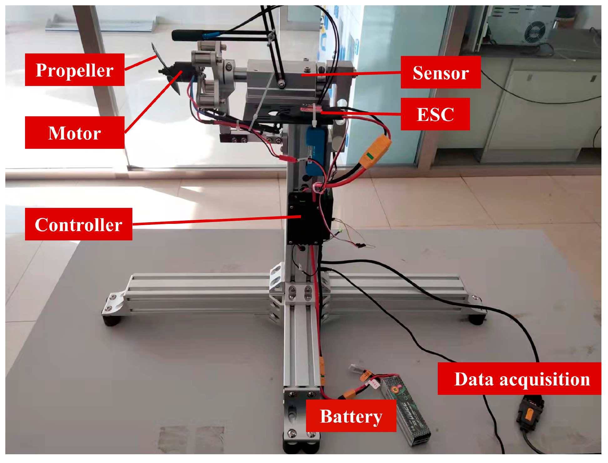
In order to acquire the aerodynamics of the propeller, an electric propulsion test bench made by the Wing-Flying company is investigated and utilized, as shown in Figure 11. Table 3 gives its nominal forces/moments and accuracy, along with the basic parameters of the test bench.
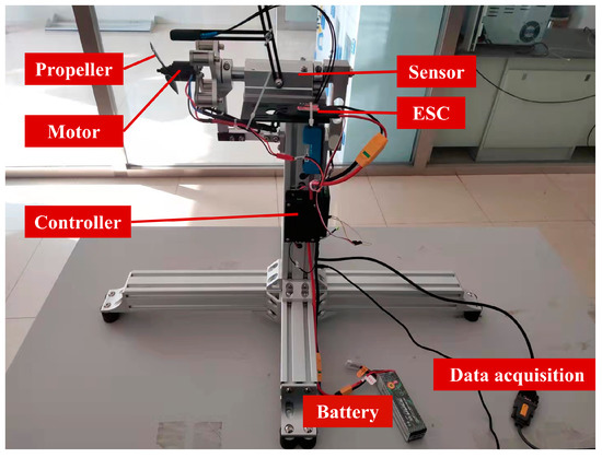
Figure 11.
Electric propulsion measurement system.
Table 3.
Specifications of the electric propulsion test bench.
Figure 12 shows the test results of the propeller, where Figure 12a is the thrust curve and Figure 12b is the torque curve. The thrust force and torque increase with the increase of the rotating speed and the fitting results are shown in Table 4 with 95% confidence bounds of KT and KM.
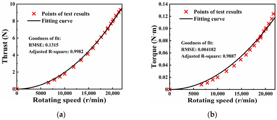
Figure 12.
Thrust and torque generated by propeller as a function of rotating speed: (a) thrust curve; (b) torque curve.
Table 4.
Test and fitting results of the propeller.
3.2.2. Motor Model
The parameters that need to be measured for the motor include the relationship between throttle and rotating speed, the response curve of the motor and the relationship between the rotating speed, torque, current and voltage. The propeller is installed on the motor in all tests. The equipment used for the motor measurement is the same as the test bench utilized for the propeller.
Figure 13 shows the relationship between the rotating speed of the motor and the throttle setting. Since the UAV usually works in the cruise status for a long time during the flight missions and the high throttle is rarely used, we limit the maximum throttle setting in the test to 0.8. The motor starts to work when the throttle increases to 0.09, and the throttle below 0.09 is the throttle dead zone. In order to simplify the modeling of the motor, the throttle–speed curve is linearly fitted.
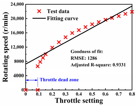
Figure 13.
Fitting curve of rotating speed versus throttle setting.
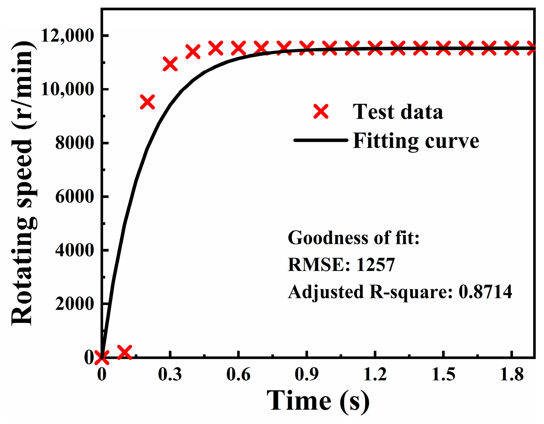
The motor is approximately a first-order system in this study and the step response curve of the motor is shown in Figure 14. It can be obtained from the response curve that the time constant Tm of the motor system is equal to 0.19 with 95% confidence bounds between 0.129 and 0.243.

Figure 14.
Step response curve of the brushless motor.
In order to calculate the energy consumption of the propulsion system, it is vital to obtain the voltage and current of the motor. In this research, the motor and ESC are simplified into one model, and the equivalent voltage and equivalent current can be calculated by Equation (15) when the thrust force and torque are given [37].
where Um0 is the nominal no-load voltage (V), Im0 is the nominal no-load current (A), Rm is the internal resistance (Ω), KV0 is the KV value of the motor (RPM/V), Mm denotes motor load torque (N·m), Nm denotes the rotating speed of the motor, which is equal to the rotating speed of the propeller (RPM). Um0 is 10 V, Im0 is 1.7A, Rm is 72.5 mΩ and KV0 is 2400 RPM/V. The model of the motor equipped in this research can be obtained as shown in Equation (16).
3.2.3. Servo Motor Model
Two DC servo motors are equipped in the UAV to drive aileron deflection and elevator deflection. The response characteristics of the servo motors will directly affect the attitude control of the UAV, so the modeling of the servo motors is very important. The modeling of the servo motor is conducted by a second-order system approach [38] and the step response is used to identify the model.
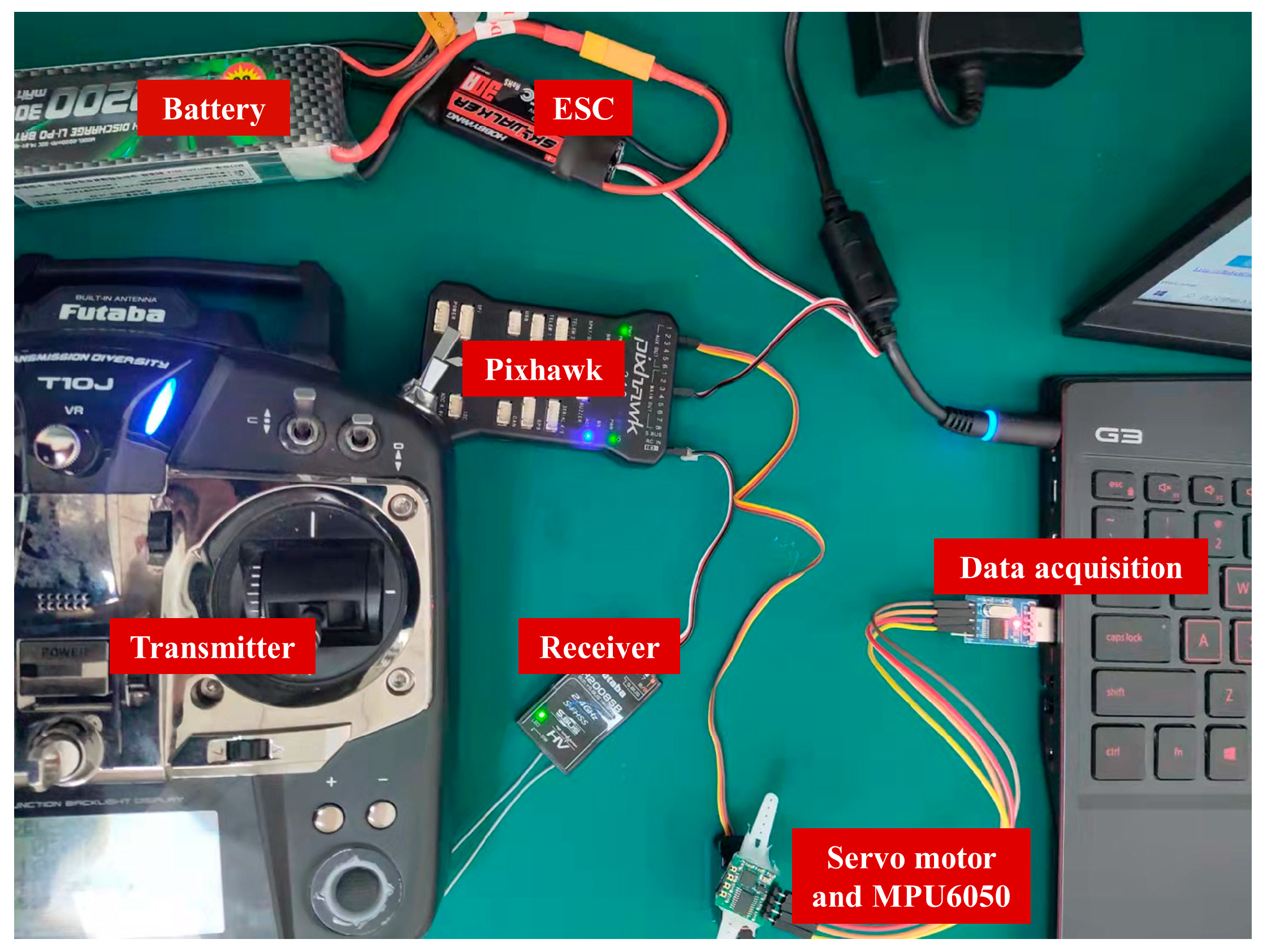
A Pixhawk flight controller equipped with a transmitter and receiver is utilized to provide PWM signal to servo motors, and an MPU6050 sensor is adopted to obtain the rotation angle, as shown in Figure 15. It should be noted that the connecting cables for data acquisition might affect the test results due to the limitation of the hardware. The magnitude of the influence caused by the cables is quite small compared to the torque of the servo motor, and we ignore it here.

Figure 15.
Measurement set-up for servo motor data acquisition.
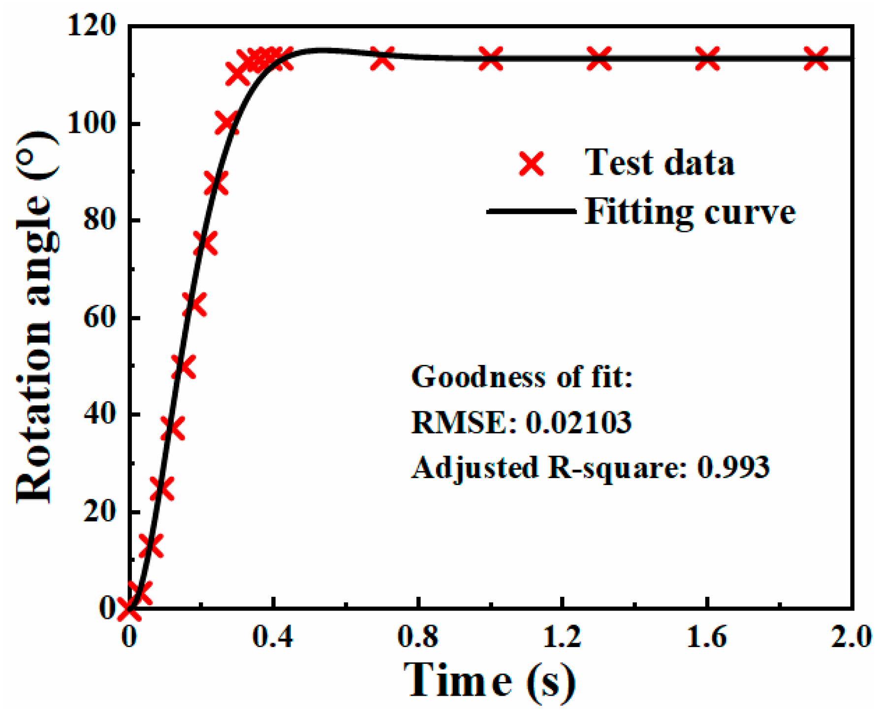
Figure 16 represents the transient state response of the rotation angle of the servo motor with a step input. The transfer function of the servo motor adopted in terms of the natural frequency and damping is shown in Equation (17).
where the natural frequency and damping of the servo motor are 9.77 and 0.801, respectively. The servo motor is an under-damped plant, and it can track the command with small oscillation.

Figure 16.
Step response curve of the servo motor.
3.2.4. Battery Model
The battery is the core and foundation of the propulsion system. Acquiring the discharge dynamics of the battery is crucial for the entire flight process. Moreover, we can also predict the endurance of the UAV for reference. A Li-Po battery was equipped and investigated in this work due to its high energy density. The main equation [39] of the battery is shown in Equation (18) and assumes the following: the temperature and the internal resistance of the battery are constant; neither the aging effect nor the Peukert effect [40] were considered.
where Vbatt denotes the battery’s actual voltage; E0 is the battery constant voltage; K is the polarization constant; C denotes the maximum battery capacity; i denotes actual constant discharge current and it is the discharged capacity; A is the exponential voltage and B represents the exponential capacity; R is the internal resistance.
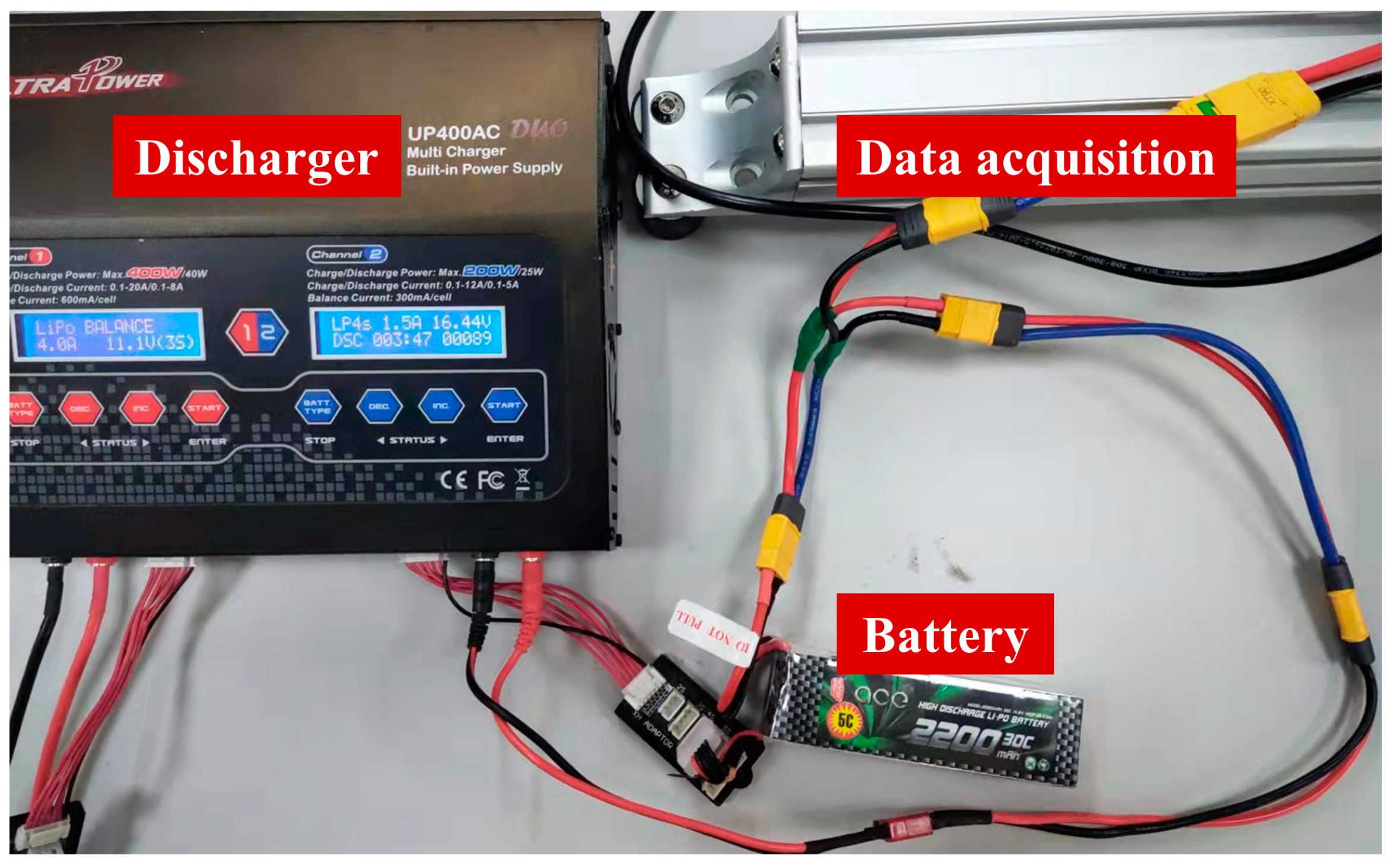
In order to obtain the battery discharge characteristics, it is necessary to record the voltage of the battery during discharging. An Ultra Power UP400AC charger was adapted to discharge the battery at a constant current. Its maximum discharge power is 40 W, and the maximum discharge current can reach 8 A. The propulsion test bench was also utilized to record the real-time voltage of the battery. Figure 17 shows the layout of the test apparatus. In this test, the battery is discharged with a constant current of 2 A until the single cell of the battery drops to 3.5 V, which is approximately completely discharged.

Figure 17.
Measurement set-up for battery data acquisition.
Figure 18a presents the experimental data and the fitted parametric curve. The parameters can be obtained by fitting the test data (time input and voltage output). Table 5 shows the optimal values of the discharge curve. The error between the predicted battery capacity and the nominal capacity is 0.41%, and the error between the predicted discharge current and the actual current is 3.95%. The obtained battery model has high accuracy. The discharge curves at different discharge rates can be simulated through the obtained battery model, as shown in Figure 18b.
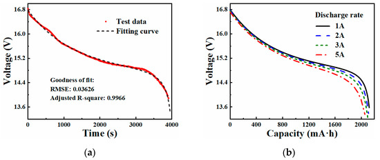
Figure 18.
Fitting and simulation of the battery model: (a) comparison of test data with the fitting curve; (b) simulation of voltage profile for different discharge rates.
Table 5.
Parameters of the battery discharge model.
3.3. Mass Moment of Inertia Measurements
Solving the moment equation requires obtaining the UAV’s mass moment of inertia. A simple approach [41] was adopted to measure the mass moment of inertia of the UAV in this work. The prototype was suspended from two points equidistant from its center of gravity. Then, the prototype was rotated by a small angle around its center of gravity and released. The moment of inertia can be calculated from the recorded oscillation period. We set a vertical rotation axis xv perpendicular to y body axis to make the angle with x body axis is αv and the angle with z body axis is 90°−αv, and the value of Ixz can be gained by Equation (19). Since the UAV is symmetrical about the x-z plane in the body frame, Ixy and Iyz can be neglected. Table 6 shows the measurement results of the UAV’s moment of inertia.
where Ixx, Iyy and Ixv are the moment of inertia of the x body axis, y body axis and xv axis, respectively.
Table 6.
Mass moment of inertia of the UAV.
3.4. Simulink Model
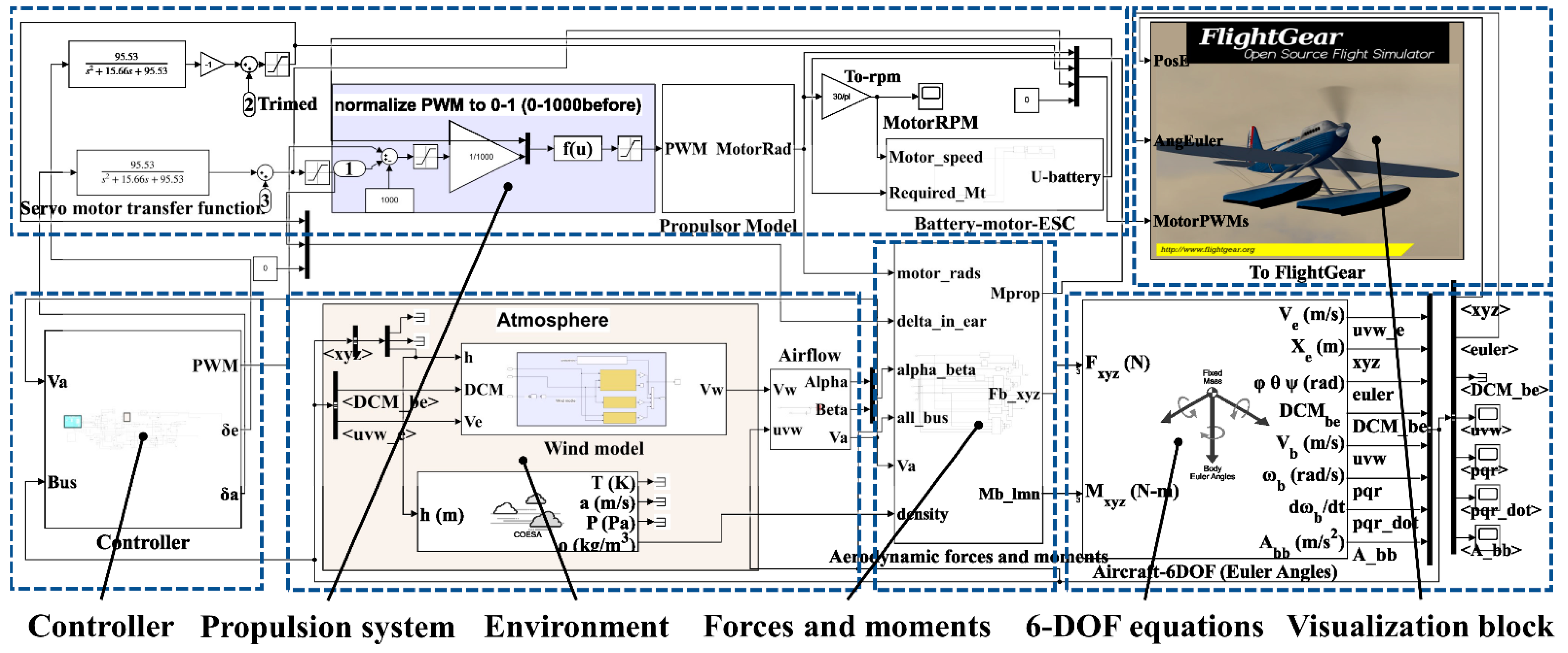
All the system parameters obtained from the simulations and experiments are imported into Simulink. The nonlinear model consists of six main blocks: the controller block, which contains stability and upper controllers; the propulsion system block, which contains the models of the propulsion system components; the environment block, which contains wind disturbances; the aerodynamic forces and moments calculation block, which calculates the aerodynamic forces and moments generated during flight; the 6-DOF equations of motion block, which contains the previously derived equations; the visualization block, which applies the co-simulation of FlightGear and MATLAB to exhibit the flight attitude of the UAV. Figure 19 shows the overall block diagram of the UAV in Simulink.
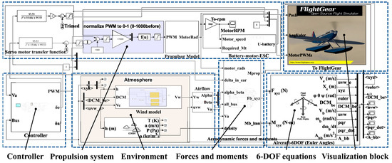
Figure 19.
The nonlinear Simulink model of the fixed-wing UAV.
4. Control Methods of the Fixed Wing UAV
Based on the established simulation model, we can efficiently design and verify the control algorithm in Simulink software. In this section, three controllers with different functions are designed to control the movement of the UAV intelligently. The simulation step is set to 1 ms and the specific simulation results are presented in the following subsections.
4.1. Stability Controller Design
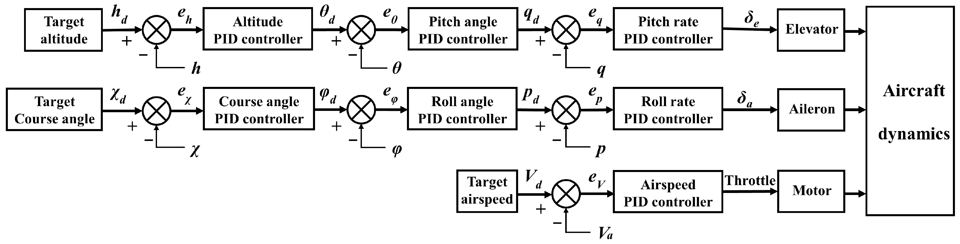
The stability controller is the most fundamental and important controller of UAV. Its performance directly determines the safety and reliability of UAVs during flight. The stability controller designed in this research can be divided into three parts: longitudinal controller, lateral controller and speed controller. The longitudinal controller includes pitch rate control, pitch angle control and height control and the lateral controller includes roll rate control, roll angle control and course angle control, while the speed controller only controls the airspeed of the aircraft. PID control method is applied to the stability controller because it is efficient and easy to implement. Figure 20 shows the specific structure of the stability controller.
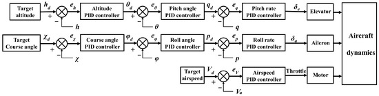
Figure 20.
Block diagram of the stability control system.
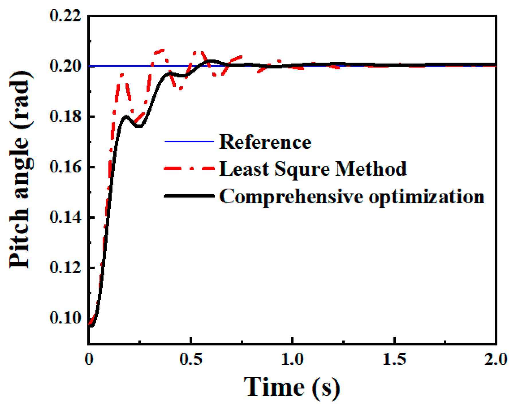
The Least Square Method based on MATLAB was employed to gain PID parameters (Kp, Ki, Kd). On the basis of the acquired PID parameters, the parameters are adjusted according to the expected performance by the Response Optimization toolbox in Simulink. The three parts of the stability controller are adjusted separately. In the longitudinal and lateral controllers, the PID parameters of the angular rate loop, angular loop and position loop are tuned successively. Figure 21 displays the step response of the pitch angle based on the Least Square Method and the toolbox. After tuning by Least Square Method, the response curve has a relatively small rise time, but a large overshoot and oscillation. The system’s overshoot and oscillation can be reduced when optimized through the toolbox. Since the PID tuning of other controllers is similar to the tuning of the pitch angle, the results will not be given here and all the parameters of the stability controller are given in Table A1 of the Appendix B.
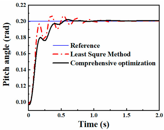
Figure 21.
Step responses of pitch angle under different methods.
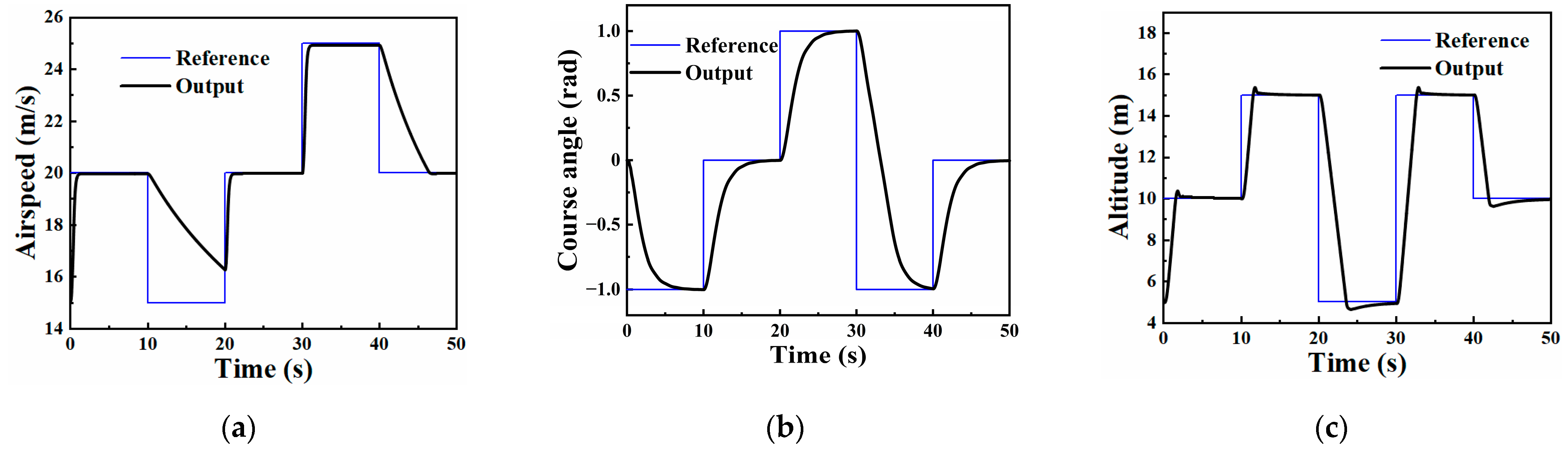
Figure 22 shows responses of the airspeed, course angle and altitude of the UAV under respective desired commands. As can be seen in Figure 22a, the UAV can quickly follow the desired command for an increase in airspeed by increasing the motor speed. However, there will be a big delay when the expected airspeed drops; this is because the airspeed of the UAV can only be reduced by wind resistance. Since the UAV investigated in this study achieves a turn by controlling the roll of the body, the tracking speed of the course angle is relatively slow, as shown in Figure 22b. Detailed step response values such as rising time, steady-state error and peak overshoot are given in Table 7 to evaluate the performance of the stability controller.
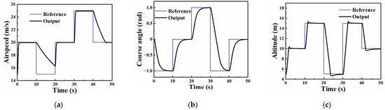
Figure 22.
Responses of the UAV under different commands: (a) airspeed; (b) course angle: (c) altitude.
Table 7.
Transient step response parameters for the stability controller.
The biggest interference encountered by the UAV during flight missions is atmospheric disturbance. Turbulence is one of the atmospheric disturbances and its effects on all parts of the fixed-wing UAV are continuous and uneven. This paper mainly studies the stability and robustness of the stability control system when the UAV encounters turbulence. For solving engineering issues, Dryden model and Von Karman model are usually implemented to simulate turbulence [42]. Dryden model is applied in this study to test and verify the controller because it is easy to implement in simulation. Dryden continuous filter can be expressed as following transfer function:
where σu, σv and σw denote turbulence intensities; Lu, Lv and Lw denote scale length. The turbulence intensities are related to flying height and typical values for wind speed at a height of 20 feet; specific parameter settings can be found in [43].
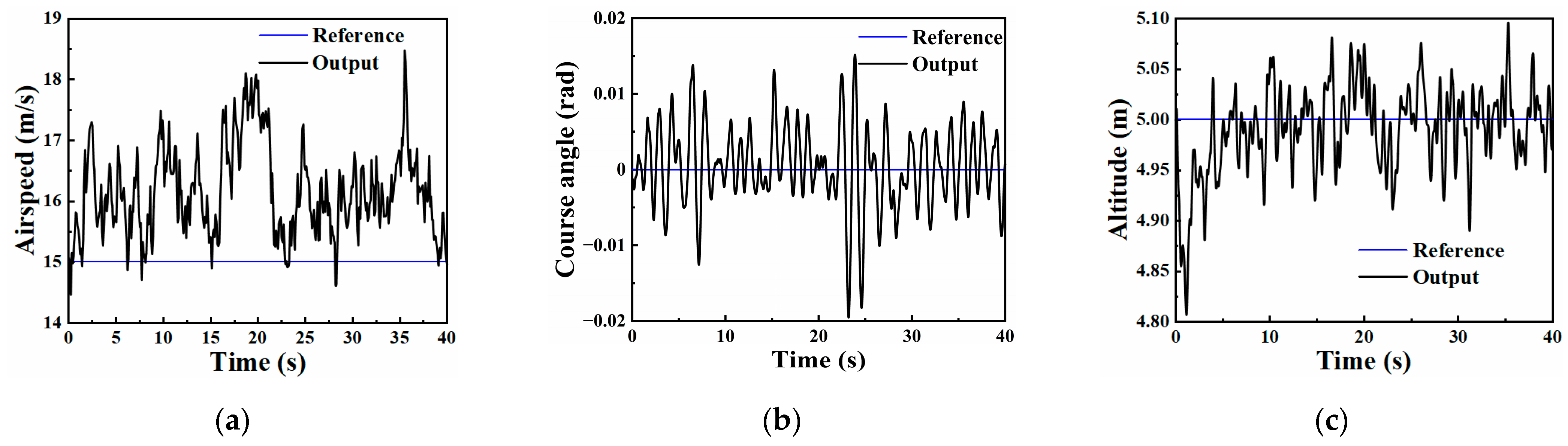
Figure 23 displays the response of the UAV’s airspeed, course angle and altitude under the effect. The airspeed is most affected by the effects of turbulence. The response of the airspeed is higher than the desired command with a maximum error of 3.5 m/s, which is because the turbulence can directly affect the airspeed and it is slow to track the descending airspeed command. The course angle and altitude will oscillate around the desired command under the influence of turbulence, and the course angle has a maximum error of 0.02 rad. Since the UAV is not in a steady state at the beginning of the simulation, it will continuously adjust to stabilize the attitude and enter the steady state at 5 s. The height error during this period is not only due to the influence of turbulence. The maximum error of height is 0.11 m at 31.2 s. The UAV system can run stably with the controller under turbulent conditions.
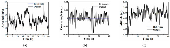
Figure 23.
Responses of the UAV under turbulent conditions: (a) airspeed; (b) course angle; (c) altitude.
4.2. Path following Controller Design
Realizing the position control of aircraft is the ultimate objective of autonomous flight control. In this part, a path following controller was designed and verified for the fixed-wing UAV based on the stability controller. The path following controller adds autonomy and intelligence to the UAV, which can make the UAV fly along a desired straight or circular path. For the UAV investigated in this study, the course angle is the basis and core of path following. The lateral distance between the UAV and the reference path can be reduced by controlling the course angle. The vector field guidance law proposed in reference [44] was investigated and implemented in this work.
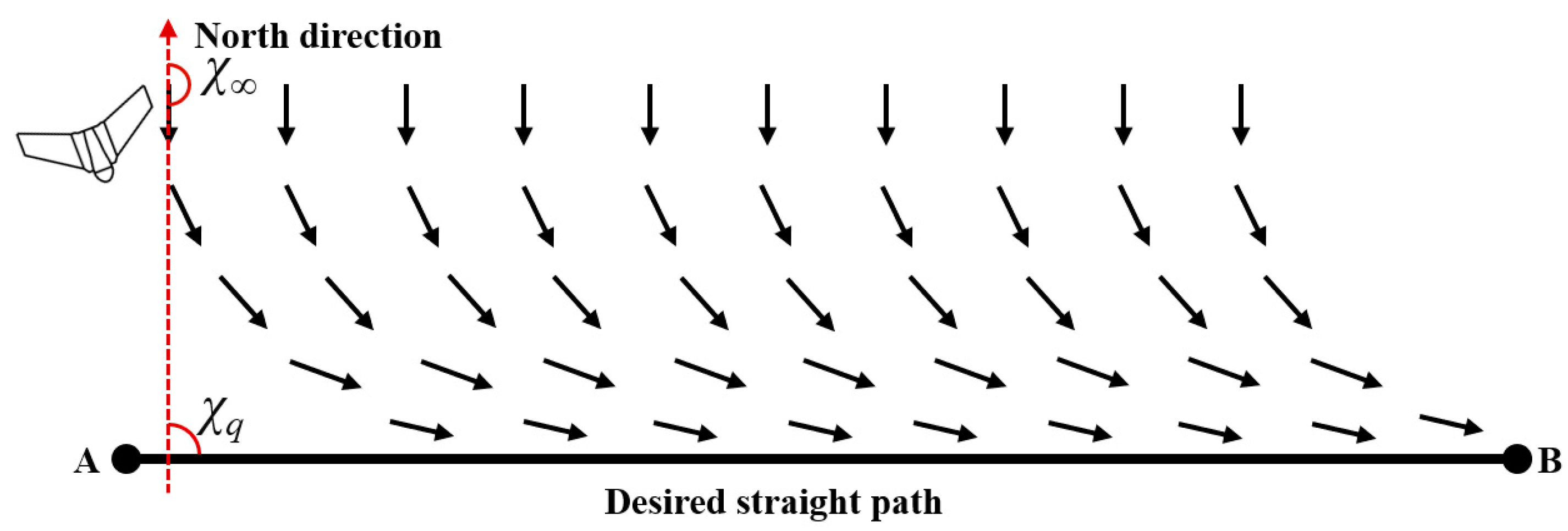
Figure 24 shows the vector field constructed by the guidance strategy when following a straight line. The UAV needs to keep tracking the direction of the vectors to make the flight direction consistent with the vector direction, and the UAV can finally fly along the desired path. The expected course angle χd of the aircraft can be expressed by Equation (21) in the vector field.
where χ∞ denotes the reference course angle far from the waypoint path; kpath denotes the turning coefficient of following a straight-line path; ey denotes the lateral distance error; χq denotes the course angle of the straight path. The values of χ∞ and kpath can affect the performance of following a straight path. Relatively appropriate values are selected for the two parameters according to the specific situation of the aircraft and the influence of different values on the flight mission is not given here.
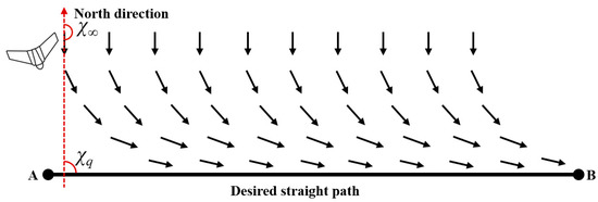
Figure 24.
Vector field of the straight path.
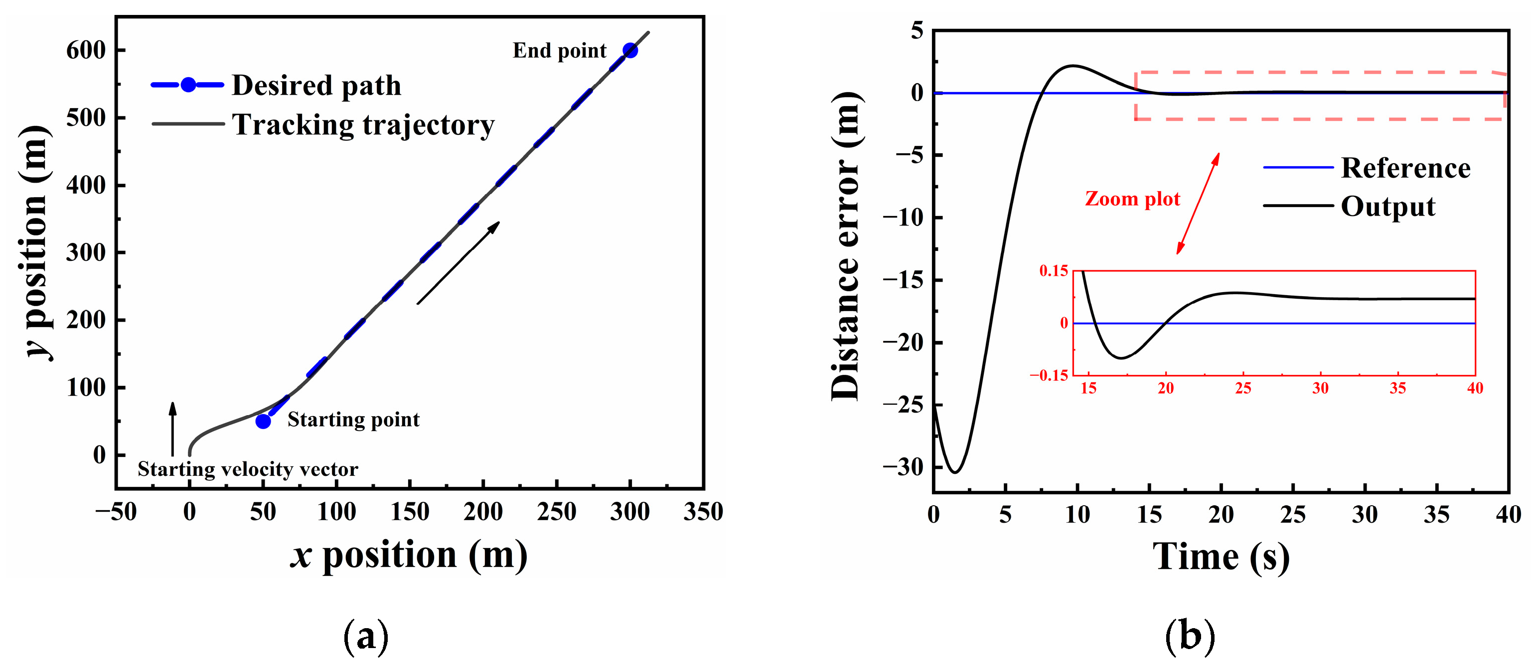
Figure 25 displays the result of the straight-line path following based on vector field guidance law, where Figure 25a shows the desired path and tracking trajectory and Figure 25b shows the distance error. It can be seen that the distance error increases in the initial stage of the simulation which is because the initial speed of the aircraft will keep the aircraft away from the path. The response curve of the distance error is not only related to the parameters of the vector field, but also closely related to the flight speed of the aircraft. In the simulation, the distance error converges towards zero with 0.1 m steady-state error when the airspeed is 15 m/s. The vector field guidance law and its parameter settings can satisfy the flight mission of following a straight-line path in this research.
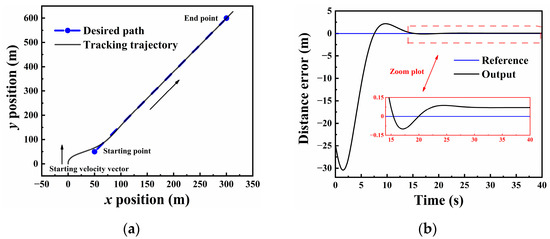
Figure 25.
Results of following a straight-line path: (a) flight trajectory; (b) distance error.
Following an orbit path is more difficult than a straight-line path. The vector field of the circular path is similar to that of the straight-line path and is not shown here. The expected course angle can be expressed by Equation (22) when following an orbit path.
where φorbit is the angle of the vector from the aircraft to the center of the circle relative to the north direction; λ is the turn direction, and λ = 1 signifies clockwise direction and λ = −1 signifies counter-clockwise direction; korbit is turning coefficient of following an orbit path; d is the distance from the aircraft to the center of the orbit path; r is the radius, r is selected as 100 m according to the flight task requirements in this paper.
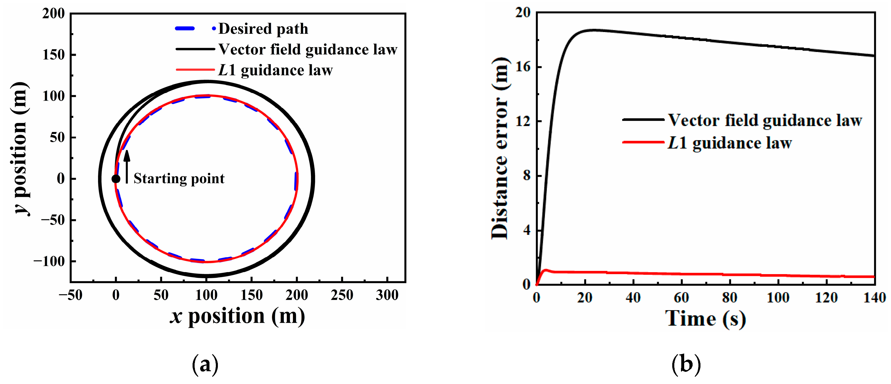
However, the application of the vector field guidance law to follow the circular trajectory has a large steady-state error in the simulation. This is because the desired course angle will change with the position of the aircraft when the aircraft follows an orbit path, and the response of the UAV to the course angle command has a certain delay, resulting in the UAV not being able to track the desired course angle in time. L1 guidance law is implemented in this work to solve the problem, and specific details of L1 guidance law can be found in reference [45]. It should be noted that relatively suitable parameters have been selected through simulation tests for the two guidance strategies, and the influence of different parameters is not given here.
Figure 26 shows the simulation results of implementing the two guidance laws to track a circular trajectory with a radius of 100 m, where Figure 26a represents the flight trajectory and Figure 26b represents the distance error. The UAV can follow the orbit path with both guidance laws. After 140 s of simulation, the distance error of the vector field guidance law is 16.83 m, while that of L1 guidance law is only 0.56 m.
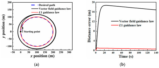
Figure 26.
Comparison of vector field guidance law and L1 guidance law: (a) flight trajectory; (b) distance error.
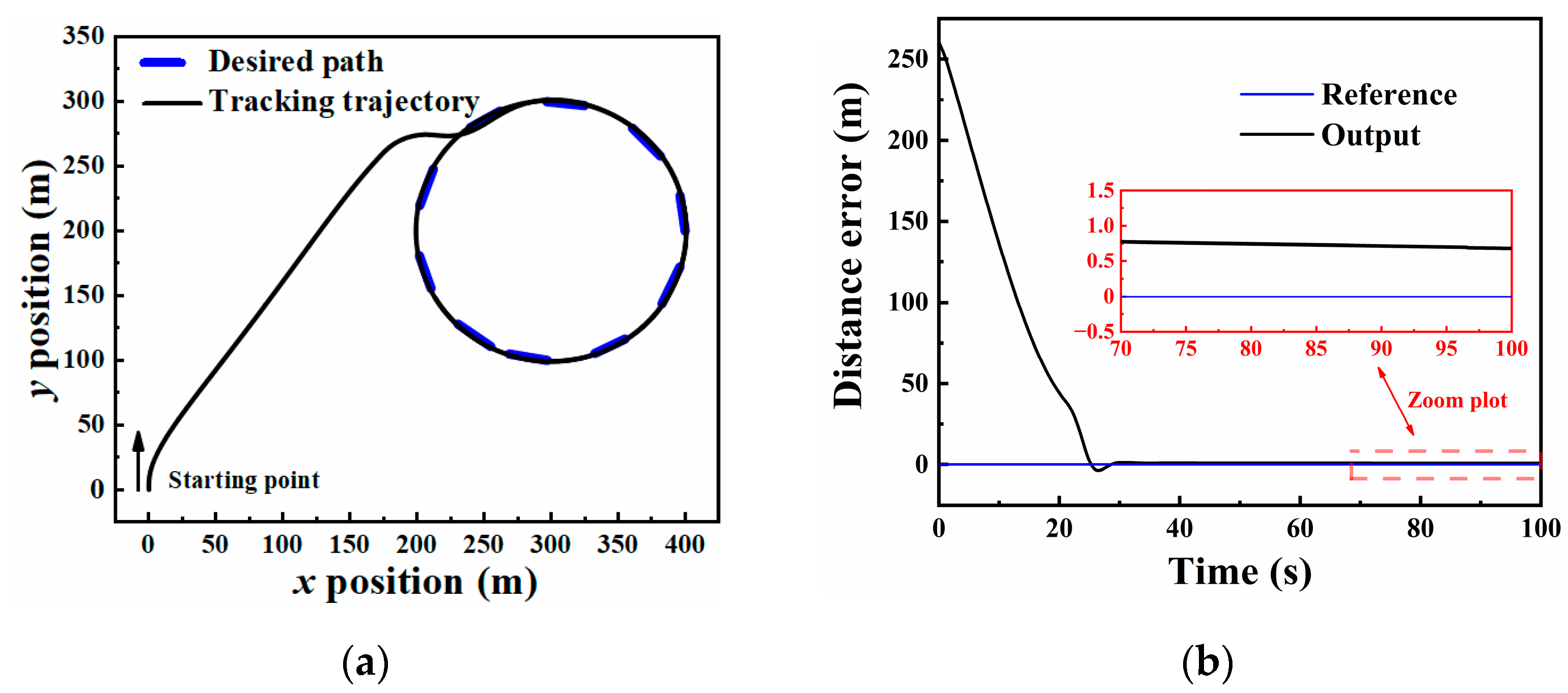
Although the application of the L1 guidance law has a smaller steady-state error, it is only suitable for the case that the aircraft is not far from the path due to some assumptions made in its derivation process. In this study, the two guidance strategies are combined. The vector field guidance law is used when the distance error is greater than 40 m, and the L1 guidance law is utilized in other cases. Figure 27 shows the flight result of the aircraft with a start point away from the orbit path, where Figure 27a shows the flight trajectory and Figure 27b shows the distance error. The steady-state error is 0.68 m during stable flight, which can meet the requirements of the flight mission.

Figure 27.
Results of following an orbit path by the combined guidance law: (a) flight trajectory; (b) distance error.
4.3. Path Management Controller Design
On the basis of the path following controller, a path management controller was designed in this part. The path management controller allows the UAV to fly between different waypoints, which can help the UAV complete some designated cruise tasks. For a path management controller, the most important thing is to determine whether the UAV has reached the previous waypoint and whether it needs to switch to the next waypoint. A simple algorithm was implemented for path management [46] in this work to accomplish the flying mission. Figure 28 shows the situation of UAV switching from one waypoint to the next waypoint.
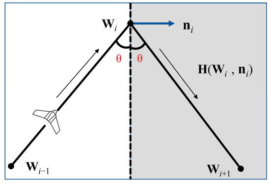
Figure 28.
Situation of UAV switching from one waypoint to the next waypoint.
At this time, the aircraft flies from point wi−1 to point wi, and vector ni can be represented by Equation (23).
where wi−1, wi, wi+1 represent the coordinates of the waypoints. H(wi, ni) is the plane perpendicular to ni through point wi. When the UAV flies over the plane H(wi, ni), which indicates that the UAV has reached waypoint wi at this time and it will fly towards the next waypoint wi+1.
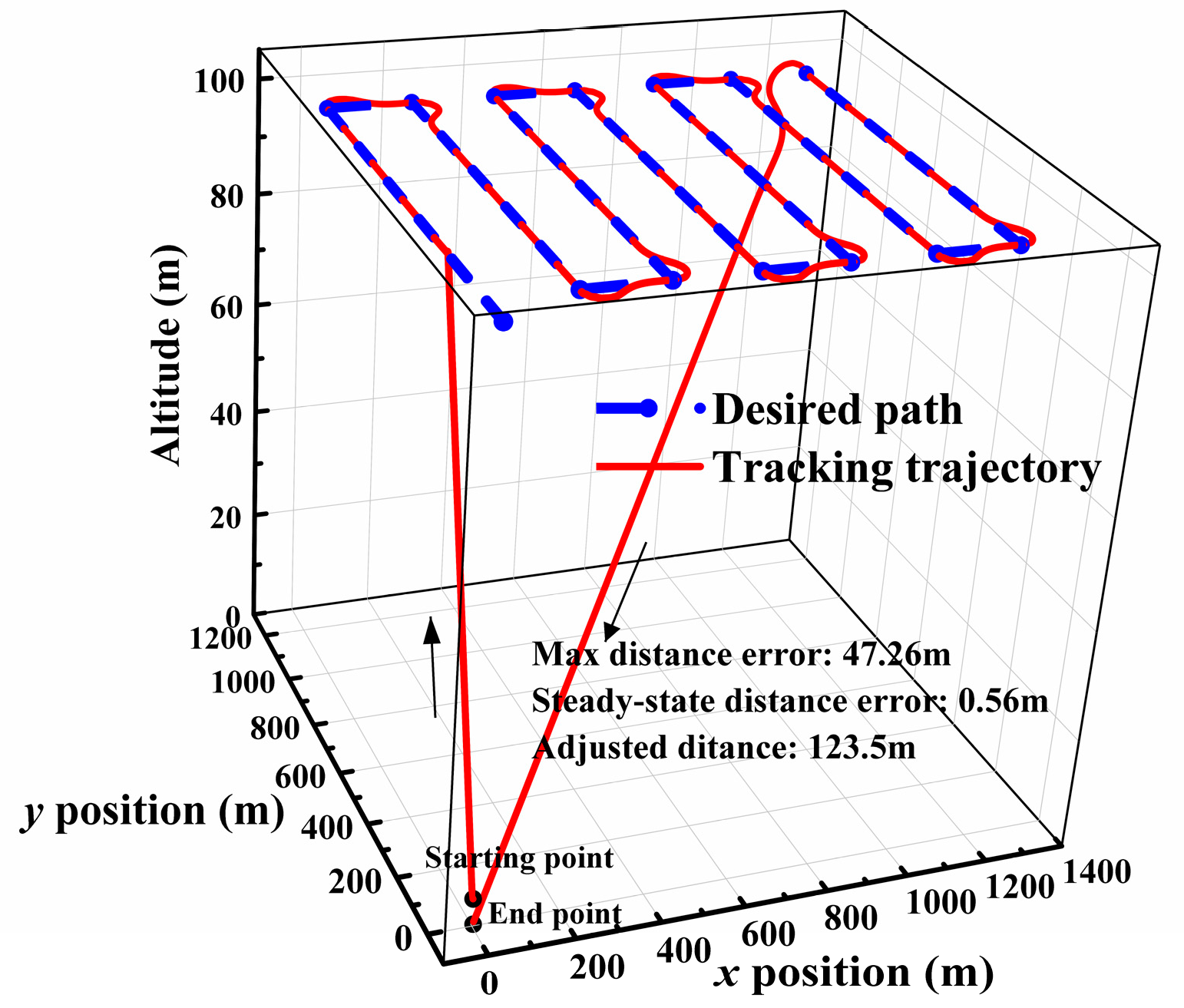
Figure 29 shows the trajectory of the aircraft and performance metrics when completing a flight mission. The aircraft starts from the starting point, climbs to the desired altitude, flies along the desired path, and finally returns to the initial waypoint. The switching between waypoints can be realized by the algorithm; however, the aircraft will fly a short distance to adjust the position when it reaches the waypoints, which is the shortcoming of the path management controller. The maximum distance error is 47.26 m when the UAV switches from one waypoint to another. Adjusted distance refers to the distance the UAV needs to fly to reduce the distance error to within 3 m.
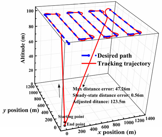
Figure 29.
Flight trajectory of completing a multi-waypoint mission.
5. Discussion
Through simulation and test results, there are some issues that need to be discussed and improved.
- Some of the aerodynamic coefficient curves obtained by the CFD method in Section 3 were simplified in order to facilitate modeling, which would bring some errors. It is an effective method to verify the CFD simulation results through additional wind tunnel tests to increase the accuracy of the aerodynamic model.
- When obtaining the parameters of the propulsion system and the servo motor through corresponding tests, the layout and performance of the test equipment might affect the test results. For example, the dynamic response of the servo motor would be affected by connecting cables used for data acquisition.
- A simple logic was used in the path management controller to determine whether the drone has reached the waypoint so that the UAV can switch to the next waypoint; however, the aircraft would fly a short distance to adjust the position when it reached the waypoint, which was the shortcoming of the path management controller.
For future work, a functional prototype will be developed and assembled, and flight tests will be conducted to evaluate the control algorithms and measure the difference between the simulation model and the real aircraft.
6. Conclusions
In this study, a complete design process was proposed and implemented for a small electric fixed-wing UAV. Firstly, 6-DOF equations of motion and nonlinear aerodynamic model of the fixed-wing UAV investigated in this work were derived, which were the basis for aircraft analysis and design.
The CFD software Fluent was used to quickly analyze the aerodynamic characteristics of the UAV and obtain the aerodynamic coefficients based on the CFD method. Among them, the rotating reference frame was applied to gain the damping derivatives by simulation of the steady movement. The parameters in the simulation were set according to the actual flight conditions, such as the angle of attack and angles of control deflections. The aerodynamic model of the UAV was well established by obtaining aerodynamic coefficients through the CFD method. The propulsion system of the aircraft was tested through different experiments, and the mathematical model of each component was established by using the test data. Some simplifications were carried out for the convenience of modeling when obtaining the motor and servo motor models. Based on Simulink software, a complete simulation model for assisting design and verifying the algorithms was quickly established by importing all the test data.
The stability controller could be well applied to the nonlinear model of the unconventional UAV with only two elevons and ensure the UAV to fly stably under the turbulent condition. Vector field guidance law and L1 guidance law were combined to follow a circular trajectory and the distance error was 0.68 m during stable flight. It could solve the problems that vector field guidance law had a large steady-state error and overcome the limitations of the assumption of the L1 guidance law. The simulation results indicate that all the control algorithms are easy to implement with excellent performance, which can meet the requirements of basic flight missions. A complete nonlinear model of the small battery-powered flying wing UAV was well established in this paper to solve the fatal problem of the small application range of the linearized model, and stability controller, path following controller and path management controller were designed and optimized. These modeling and control methods of the small electric fixed-wing UAV can provide some reference for relevant designers. In addition, all the UAV parameters measured in our work are presented in this paper, which can be used to assist in the design of the controller and verify the effectiveness of the control algorithm.
Author Contributions
Conceptualization, H.Z. and Y.W.; methodology, Y.W.; software, Y.W.; validation, H.Z., Y.W. and Z.Z.; formal analysis, C.Z.; investigation, H.Z.; resources, Z.Z.; data curation, C.Z.; writing—original draft preparation, Y.W.; writing—review and editing, Y.W. and Y.L.; visualization, Z.Z.; supervision, H.Z.; project administration, H.Z.; funding acquisition, H.Z. All authors have read and agreed to the published version of the manuscript.
Funding
This research was funded by Jilin Province Key R&D Plan Project under Grant, grant number 20200401113GX.
Institutional Review Board Statement
Not applicable.
Informed Consent Statement
Not applicable.
Data Availability Statement
The data presented in this study are available on request from the corresponding author.
Conflicts of Interest
The authors declare no conflict of interest.
Appendix A. Detailed Transformation Matrices of the UAV’s Mathematical Model
The detailed expression of the transformation matrix from the body axis to Earth axis is shown in (A1).
The detailed expression of transformation matrix from angular velocities to Euler rates is shown in (A2).
The detailed expression of transformation matrix from wind axis to body axis is shown in (A3).
Appendix B. Stability Controller Parameters
Table A1.
Parameters of stability controller.
Table A1.
Parameters of stability controller.
| Parameter | Kp | Ki | Kd | |
|---|---|---|---|---|
| Longitudinal | Pitch rate | 0.3889 | 7.5461 | 0.0661 |
| Pitch angle | 8.2978 | 0.2536 | 0.1088 | |
| Altitude | 0.6879 | 0.2373 | 0.1282 | |
| Lateral | Roll rate | 0.2631 | 5.5033 | 0.047 |
| Roll angle | 22.2973 | 0.0329 | 0.7683 | |
| Course angle | 1.02 | 0.0011 | 0 | |
| Throttle | Airspeed | 1.4665 | 0 | 0.2171 |
References
- Colomina, I.; Molina, P. Unmanned aerial systems for photogrammetry and remote sensing: A review. J. Photogramm. Remote Sens. 2014, 92, 79–97. [Google Scholar] [CrossRef] [Green Version]
- Psirofonia, P.; Samaritakis, V.; Eliopoulos, P.; Potamitis, I. Use of Unmanned Aerial Vehicles for agricultural applications with emphasis on crop protection: Three novel case-studies. Int. J. Agric. Sci. 2017, 5, 30–39. [Google Scholar] [CrossRef]
- Triputra, F.R.; Trilaksono, B.R.; Adiono, T.; Sasongko, R.A.; Dahsyat, M. Nonlinear dynamic modeling of a fixed-wing Unmanned Aerial Vehicle: A case study of Wulung. J. Mechatron. Electr. Power Veh. Technol. 2015, 6, 19–30. [Google Scholar] [CrossRef] [Green Version]
- Zhang, H.; Wang, L.; Tian, T.; Yin, J. A review of Unmanned Aerial Vehicle Low-Altitude Remote Sensing (UAV-LARS) Use in agricultural monitoring in China. Remote Sens. 2021, 13, 1221. [Google Scholar] [CrossRef]
- Turner, D.; Lucieer, A.; Malenovský, Z.; King, D.H.; Robinson, S.A. Spatial co-registration of ultra-high resolution visible, multispectral and thermal images acquired with a micro-UAV over Antarctic moss beds. Remote Sens. 2014, 6, 4003–4024. [Google Scholar] [CrossRef] [Green Version]
- Marinello, F.; Pezzuolo, A.; Chiumenti, A.; Sartori, L. Technical analysis of Unmanned Aerial Vehicles (Drones) for agricultural applications. In Proceedings of the 15th International Scientific Conference on Engineering for Rural Development, Jelgava, Latvia, 25–27 May 2016; pp. 870–875. [Google Scholar]
- Boon, M.A.; Drijfhout, A.P.; Tesfamichael, S. Comparison of a fixed-wing and multi-rotor UAV for environmental mapping applications: A case study. In Proceedings of the International Conference on Unmanned Aerial Vehicles in Geomatics, Bonn, Germany, 4–7 September 2017; pp. 47–54. [Google Scholar]
- Panagiotou, P.; Kaparos, P.; Yakinthos, K. Wing let design and optimization for a MALE UAV using CFD. Aerosp. Sci. Technol. 2014, 39, 190–205. [Google Scholar] [CrossRef]
- Tan, B.; Ma, J.; Zhang, Y. Analysis of aerodynamic characteristics for a flying-wing UAV with asymmetric wing damage. In Proceedings of the 2018 33rd Youth Academic Annual Conference of Chinese Association of Automation (YAC), Nanjing, China, 18–20 May 2018; pp. 276–280. [Google Scholar]
- Hassanalian, M.; Abdelkefi, A. Design, manufacturing, and flight testing of a fixed wing Micro Air Vehicle with Zimmerman planform. Meccanica 2017, 52, 1265–1282. [Google Scholar] [CrossRef]
- Chung, P.-H.; Ma, D.-M.; Shiau, J.-K. Design, manufacturing, and flight testing of an experimental flying wing UAV. Appl. Sci. 2019, 9, 3043. [Google Scholar] [CrossRef] [Green Version]
- Aboelezz, A.; Hassanalian, M.; Desoki, A.; Elhadidi, B.; El-Bayoumi, G. Design, experimental investigation, and nonlinear flight dynamics with atmospheric disturbances of a fixed-wing Micro Air Vehicle. Aerosp. Sci. Technol. 2020, 97, 105636. [Google Scholar] [CrossRef]
- Saderla, S.; Rajaram, D.; Ghosh, A.K. Parameter estimation of unmanned flight vehicle using wind tunnel testing and real flight data. J. Aerosp. Eng. 2017, 30, 04016078. [Google Scholar] [CrossRef]
- Priyambodo, T.K.; Majid, A. Modeling and simulation of the UX-6 fixed-wing Unmanned Aerial Vehicle. J. Control Autom. Electr. Syst. 2021, 32, 1344–1355. [Google Scholar] [CrossRef]
- Kandath, H.; Pushpangathan, J.V.; Bera, T.; Dhall, S.; Bhat, M.S. Modeling and closed loop flight testing of a fixed wing Micro Air Vehicle. Micromachines 2018, 9, 111. [Google Scholar] [CrossRef] [Green Version]
- Farhadi, R.M.; Kortunov, V.; Molchanov, A.; Solianyk, T. Estimation of the lateral aerodynamic coefficients for Skywalker X8 flying wing from real flight-test data. Acta Polytech. 2018, 58, 77–91. [Google Scholar] [CrossRef] [Green Version]
- Kim, C.; Chung, J.D. Aerodynamic analysis of tilt-rotor Unmanned Aerial Vehicle with computational fluid dynamics. J. Mech. Sci. Technol. 2006, 20, 561–568. [Google Scholar] [CrossRef]
- Safi’i, I.; Nurohman, C.; Hardy, D.D.A.; Arifianto, O.; Muhammad, H. Thrust modelling for a small UAV. In Proceedings of the 7th Annual International Seminar on Aerospace Science and Technology (ISAST), Jakarta, Indonesia, 24–25 September 2019. [Google Scholar]
- Zhao, A.; Zhang, J.; Li, K.; Wen, D. Design and implementation of an innovative airborne electric propulsion measure system of fixed-wing UAV. Aerosp. Sci. Technol. 2021, 109, 106357. [Google Scholar] [CrossRef]
- Piljek, P.; Kotarski, D.; Krznar, M. Method for characterization of a multirotor UAV electric propulsion system. Appl. Sci. 2020, 10, 8229. [Google Scholar] [CrossRef]
- Virginio, R.; Fuad, F.A.; Jihadil, M.; Ramadhani, M.J.; Rafie, M.; Stevenson, R.; Adiprawita, W. Design and implementation of low cost thrust benchmarking system (TBS) in application for small scale electric UAV propeller characterization. In Proceedings of the 6th International Seminar on Aerospace Science and Technology (ISAST), Jakarta, Indonesia, 25–26 September 2018. [Google Scholar]
- Ulus, S.; Eski, I. Neural network and fuzzy logic-based hybrid attitude controller designs of a fixed-wing UAV. Neural Comput. Appl. 2021, 33, 8821–8843. [Google Scholar] [CrossRef]
- Ulker, H.; Baykara, C.; Ozsoy, C. Design of MPCs for a fixed wing UAV. Aircr. Eng. Aerosp. Technol. 2017, 89, 893–901. [Google Scholar] [CrossRef]
- Melkou, L.; Rezoug, A.; Hamerlain, M. PID-terminal sliding mode control of aircraft UAV. In Proceedings of the 8th UKSim-AMSS European Modelling Symposium on Computer Modelling and Simulation (EMS), Pisa, Italy, 21–23 October 2014; pp. 233–238. [Google Scholar]
- Aboelezz, A.; Mohamady, O.; Hassanalian, M.; Elhadidi, B. Nonlinear flight dynamics and control of a fixed-wing Micro Air Vehicle: Numerical, system identification and experimental investigations. J. Intell. Robot. Syst. 2021, 101, 64. [Google Scholar] [CrossRef]
- Sadraey, M.H. Aircraft Design: A Systems Engineering Approach; John Wiley & Sons: Hoboken, NJ, USA, 2012. [Google Scholar]
- Cinar, G.; Emeneth, M.; Mavris, D.N. A methodology for sizing and analysis of electric propulsion subsystems for Unmanned Aerial Vehicles. In Proceedings of the 54th AIAA Aerospace Sciences Meeting, San Diego, CA, USA, 4–8 January 2016; p. 216. [Google Scholar]
- Avanzini, G.; de Angelis, E.L.; Giulietti, F. Optimal performance and sizing of a battery-powered aircraft. Aerosp. Sci. Technol. 2016, 59, 132–144. [Google Scholar] [CrossRef]
- Zhu, H.; Wang, Y.; Lan, Y.; Zhang, C.; Li, K. Design and simulation of long-endurance and light agricultural remote sensing fixed-wing UAV. Trans. Chin. Soc. Agric. Mach. 2021, 52, 234–242. (In Chinese) [Google Scholar]
- Etkin, B.; Reid, L.D. Dynamics of Flight; John Wiley & Sons: Hoboken, NJ, USA, 1959. [Google Scholar]
- Pushpangathan, J.V.; Bhat, M.S.; Harikumar, K. Effects of gyroscopic coupling and countertorque in a fixed-wing Nano Air Vehicle. J. Aircr. 2018, 55, 239–250. [Google Scholar] [CrossRef]
- Gryte, K.; Hann, R.; Alam, M.; Rohac, J.; Johansen, T.A.; Fossen, T.I. Aerodynamic modeling of the Skywalker X8 Fixed-Wing Unmanned Aerial Vehicle. In Proceedings of the International Conference on Unmanned Aircraft Systems (Icuas), Dallas, TX, USA, 12–15 June 2018; pp. 826–835. [Google Scholar]
- Su, H.; Bao, X.; Li, J.; Liu, K.; Cen, M.; Song, J. Calculation and analysis on stealth and aerodynamics characteristics of a medium altitude long endurance UAV. Procedia Eng. 2015, 99, 111–115. [Google Scholar]
- Ye, C.; Ma, D. Aircraft dynamic derivatives calculation using CFD techniques. J. Beijing Univ. Aeronaut. Astronaut. 2013, 39, 196–219. (In Chinese) [Google Scholar]
- Jung, D.; Tsiotras, P. Modeling and hardware-in-the-loop simulation for a small unmanned aerial vehicle. In Proceedings of the AIAA Infotech@ Aerospace 2007 Conference and Exhibit, Rohnert Park, CA, USA, 7–10 May 2007; p. 2768. [Google Scholar]
- Moffitt, B.; Bradley, T.; Parekh, D.; Mavris, D. Validation of vortex propeller theory for UAV design with uncertainty analysis. In Proceedings of the 46th AIAA Aerospace Sciences Meeting and Exhibit, Reno, NV, USA, 7–10 January 2008; p. 406. [Google Scholar]
- Quan, Q. Introduction to Multicopter Design and Control; Springer: Singapore, 2017. [Google Scholar]
- Sufendi; Trilaksono, B.R.; Nasution, S.H.; Purwanto, E.B. Design and implementation of hardware-in-the-loop-simulation for UAV using PID control method. In Proceedings of the 3rd International Conference on Instrumentation, Communications, Information Technology, and Biomedical Engineering (ICICI-BME), Bandung, Indonesia, 7–8 November 2013; pp. 124–130. [Google Scholar]
- Mariga, L.; Silva Tiburcio, I.; Martins, C.A.; Almeida Prado, A.N.; Nascimento Jr, C. Measuring battery discharge characteristics for accurate UAV endurance estimation. Aeronaut. J. 2020, 124, 1099–1113. [Google Scholar] [CrossRef]
- Sun, Y.-H.; Jou, H.-L.; Wu, J.-C. Multilevel Peukert equations based residual capacity estimation method for Lead-Acid battery. In Proceedings of the IEEE International Conference on Sustainable Energy Technologies, Singapore, 24–27 November 2008; pp. 101–105. [Google Scholar]
- McClelland, W.A. Inertia Measurement and Dynamic Stability Analysis of a Radio-Controlled Joined-Wing Aircraft. Master’s Thesis, Air Force Institute of Technology, Greene, OH, USA, 2006. [Google Scholar]
- Wang, B.; Ali, Z.A.; Wang, D. Controller for UAV to oppose different kinds of wind in the environment. J. Control Sci. Eng. 2020, 2020. [Google Scholar] [CrossRef]
- Hakim, T.M.I.; Arifianto, O. Implementation of Dryden continuous turbulence model into simulink for LSA-02 flight test simulation. In Proceedings of the 5th International Seminar on Aerospace Science and Technology (ISAST), Medan, Indonesia, 27–29 September 2017. [Google Scholar]
- Lawrence, D.; Frew, E.; Pisano, W. Lyapunov vector fields for autonomous UAV flight control. In Proceedings of the AIAA Guidance, Navigation and Control Conference and Exhibit, Hilton Head, SC, USA, 20–23 August 2007; p. 6317. [Google Scholar]
- Park, S.; Deyst, J.; How, J. A new nonlinear guidance logic for trajectory tracking. In Proceedings of the AIAA Guidance, Navigation, and Control Conference and Exhibit, Providence, RI, USA, 16–19 August 2004; p. 4900. [Google Scholar]
- Beard, R.W.; McLain, T.W. Small Unmanned Aircraft: Theory and Practice; Princeton University Press: Princeton, NJ, USA, 2012. [Google Scholar]


Publisher’s Note: MDPI stays neutral with regard to jurisdictional claims in published maps and institutional affiliations. |
© 2021 by the authors. Licensee MDPI, Basel, Switzerland. This article is an open access article distributed under the terms and conditions of the Creative Commons Attribution (CC BY) license (https://creativecommons.org/licenses/by/4.0/).