Abstract
This paper is focused on the stabilization of Takagi–Sugeno fuzzy model-based Markovian jump systems with the aid of a delayed state observer. Due to network-induced constraints in the communication channel, a delay partition method combined with an event-triggered mechanism is proposed to design the observer. Then, a novel integral sliding surface is designed, based on which sliding mode dynamics is obtained. Further, according to stochastic stability theory, feasible conditions are provided to ensure the sliding mode dynamics and the error dynamics have an H∞ attenuate level γ. The challenge is to deal with the issue that transition rates may be totally unknown. Moreover, an observer-based sliding mode controller is constructed to ensure the finite-time reachability of the predefined sliding surface. Finally, a numerical example based on a robotic manipulator is given to verify the effectiveness of the proposed method.
1. Introduction
With the strong demands for modeling a physical system with high accuracy, for instance, the physical systems may have structural mutation due to changes of power, the shift of parameters and external disturbances, etc., which provoke the need to seek for more suitable mathematical models. Therefore, Markovian jump systems (MJSs) have attracted numerous attention because of its ability to model such kind of physical model with multi-modal characteristics or intelligent control system with multi-controller switching [1]. So far, the researches on MJSs have been reported by many in both applications and theoretical aspects, such as the Markov jump models are widely applied in nuclear power systems, manufactory and network communication [2,3,4,5], etc. Theoretically, it also witnessed the issue of stochastic stability analysis, stabilization, filter design and so on. For example, in [6], the robust stability and control of uncertain discrete-time linear systems with Markovian jumping parameters was dealt with; in [7], the problems of stochastic stabilization and H∞ control for 2-D MJSs were proposed; and systematic theory on stochastic differential equations with Markovian switching was presented in [8]; the H∞ filtering problem for MJSs was studied in [9,10]; for more details, we may refer to [11,12,13,14,15] and some of their references. In another aspect, due to the existence of nonlinearity, the Takagi–Sugeno (T-S) fuzzy modeling approach has become one of the most popular and effective ways to handle the synthesis of complex nonlinear systems [16], and the investigation on T-S fuzzy model-based MJSs is also rich. In addition, the stabilization of nonlinear singular MJS with matched/unmatched uncertainties based on the T-S fuzzy model was studied in [17]; the robust H∞ control involving a class of uncertain stochastic MJSs was investigated in [18], etc. [19,20,21]. As we all know, the transition rates (TRs) play a big role in the system’s performance, but getting exact TR information seems impossible due to all kinds of limits in actual systems, such as high cost, technique limitations and so on. Hence, it is necessary to study MJSs in the presence of deficient TR information. Up to now, some results can be found in dealing with this issue, but not enough. For example, some pioneer works dealt with the issues of stabilization, stochastic stability and quantized filtering for (singular) MJSs with deficiency mode information in [22,23,24,25]. However, all the results proposed in literature [22,23,24,25] need TR information, no matter partially or fully. So, what if the information of TRs for one mode to another is completely unknown? This is the new challenge we are going to deal with in this paper.
Sliding mode control (SMC) has exclusive advantages in dealing with the nonlinear complex system, such as the good transient performance, fast response speed and strong robustness, which has attracted great attention in the community since its appearance. The researches on SMC of MJSs were also active, for instance, a class of continuous-time MJSs with digital communication constraints via SMC approach was proposed in [26]; the robust H∞ SMC for discrete-time MJSs subject to intermittent observations was researched in [27]; in Ref. [28], the research of asynchronous SMC was investigated based on uncertain MJSs with time-varying delays. In the presence of status components unavailable, observer-based SMC arises, such as an adaptive sliding mode observer was designed for nonlinear MJSs in [29]; the research about sensor fault estimation along with fault-tolerant control for time-delay MJSs through sliding mode observer technique was studied in [30]; in [31], a reduced-order sliding mode observer was designed to realize adaptive control of T-S fuzzy modeled-based MJSs. More works can be found in [32,33,34] and references therein.
At present, the control systems are realized by distributed components connected through the network, which could improve efficiency and reliability. Traditionally, the time-triggered control is performed periodically that may bring a heavy communication burden. Recently, the event-triggered control strategy has attracted numerous attention for the transmission of data only allowed when it is necessary, which could save communication resources and make full use of congested network channel. Therefore, the approach of event-triggered control is becoming more and more popular, and the results have been reported involving continuous-time and discrete-time systems [35,36,37,38], multi-agent systems [39], stochastic systems [40] and neural networks [41], etc. Recently, the event-triggered based SMC was also touched in the field, such as the event-triggered SMC for stochastic systems on the way of output feedback was studied in [42], etc. However, the problem of observer-based SMC through event-triggered mechanism is seldom touched yet since such an issue is a difficulty due to network-induced constraints. For instance, how to overcome the network-induced delays in constructing desire state observer in order to realize good approximation of original state, and how to design sliding surface to accommodate the sliding motion have partially stimulated our research.
Briefly speaking, this paper will handle the problem of how to design a sliding mode observer for stabilization of nonlinear MJSs based on T-S fuzzy modeling approach. Most of main attention will be focused on designing an event-triggered based time-delay sliding mode observer and a novel sliding mode surface, then establishing feasible easy-checking LMI conditions to ensure H∞ performance in sliding mode dynamics and error dynamics with totally unknown mode transition information. The main contributions of this paper can be concluded as: (1) Compared with traditional observer, the proposed event-triggered time-delay state observer brings the benefits that error is better suppressed and better stabilization property is obtained; (2) a novel sliding surface function is proposed, based on which the observer gain matrices can be computed in the design process rather than given as in [42]; (3) a new method is proposed to give feasible strict LMI conditions for stability of MJSs with totally unknown transition information; and (4) fuzzy SMC law ensures finite-time reachability of sliding surface and keeps sliding motion of each sub-models in the presence of uncertain transition information and nonlinearities.
Notions:
In this paper, the concept denotes is a positive definite (positive semidefinite) matrix. and represent an identity matrix and zero matrix, respectively. represents the expectation operator about probability measures. represents the Euclidean vector norm. denotes Symmetric elements in a symmetric matrix. expresses .
2. Model Establishing and Problem Statement
Let us consider the model of single-link robot arm model proposed in [43], where the equation of dynamic is given by
the meanings of parameters are defined in Table 1.

Table 1.
NOTATIONS.
Letting and . According to the method proposed in [44] that under certain angle position, the nonlinearity can be replaced by
in which is a known parameter and the membership functions satisfy with . By solving the above equation, the membership functions and are obtained as
Based on the membership function mentioned above, it is easy to see that if is about 0 rad, then , , if is about or rad, then and . Hence, the fuzzy model-based state-space description of the robotic system can be rewritten as:
Plant Rule 1: IF is “about 0 rad”,
THEN
where and
Particularly, as discussed in [43], the moment of inertia may change due to the abrupt change of actual operating, for instance, the switching of the parameters follows the Markovian jumping rules. Therefore, based on the above model, let us consider the following general model:
Plant Rule i: IF is and is and … and is
THEN
where denotes the state vector; are premise variables; (; ) are fuzzy sets, is the control input; is the controlled output. and are the system matrices with appropriate dimensions; is the input matrix with full column rank. The process of stochastic jumping is a continuous-time homogenous Markovian jumping process. The process of generator with values in a finite set given by
where and , ,, is the transition rate from mode at time to mode at time . Meanwhile, for each .
Through fuzzy standard blending, the model can be easily derived:
in which , is the membership function that the formula of which is
where is the rank of membership of in . In addition, for all , it is satisfied that and . For simplicity, and is short for in the following.
The following Definitions and Lemma are introduced.
Definition 1.
([45]) Given the Lyapunov functional candidate with twice differentiable on , then, which is infinitesimal operator is given by
Definition 2.
([46]) The unforced stochastic system (2) (i.e., ) is said to be stochastically stable for any initial condition and
, as long as it satisfies
Lemma 1.
([47]) Given any real number and any square matrix , for any matrix , the matrix inequality holds.
Here, in this paper, an appropriate observer-based fuzzy SMC strategy for the model (2) on the communication networks with network-induced constraints has been designed to obtain good stochastic stability property with an H∞ performance in sliding mode dynamics and error dynamics.
3. Main Results
Given that the state component may not be accessible in practice, a state observer needs to be designed first. Through digital communication medium, the signal is transmitted in the output channel of observer that may suffer from network-induced delays, where the output measurement sampled periodically with sampling period . Here, () is the current measurement and (, , is triggering time) is the one latest transmitted, respectively. The judgement condition whether retrieving the transmission is determined by the following conditions:
where is a positive definite weighting matrix decided by the error tolerance .
The transmission scheme in the next transmission instant is determined by
Remark 1.
From the above triggered mechanism,only meeting the triggering condition that data packets sampled will be sent on the network; therefore, the network efficiency is improved. In particular, if , it is seen that the data transmission mechanism is simplified from event triggering to periodic triggering.
3.1. Network and ZOH
Due to network transmission speed, network transmission protocol and the load connected in the network, the network-induced delays are considered first, the released transmission delay in kth is marked as , that is, , where is the instance that the measurement arrived ZOH. Let be the maximum transmission delay, i.e., . Therefore, the interval of time can be divided into subintervals as follows:
where is determined by . Then
Denote
Obviously,
Now, define
which combines with (9) leads to
Given the triggering situation (7), satisfies that
In addition, as shown in Figure 1 that the input in state observer satisfies
that is the received signal equals to the signal released at instants of event-triggering . The output signal from ZOH is piecewise constant but continuous from the right. Thanks to the characteristics of ZOH causal reconstruction, it is convenient to carry out the design of observer and the analysis of sliding motion.
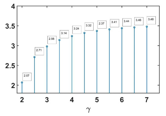
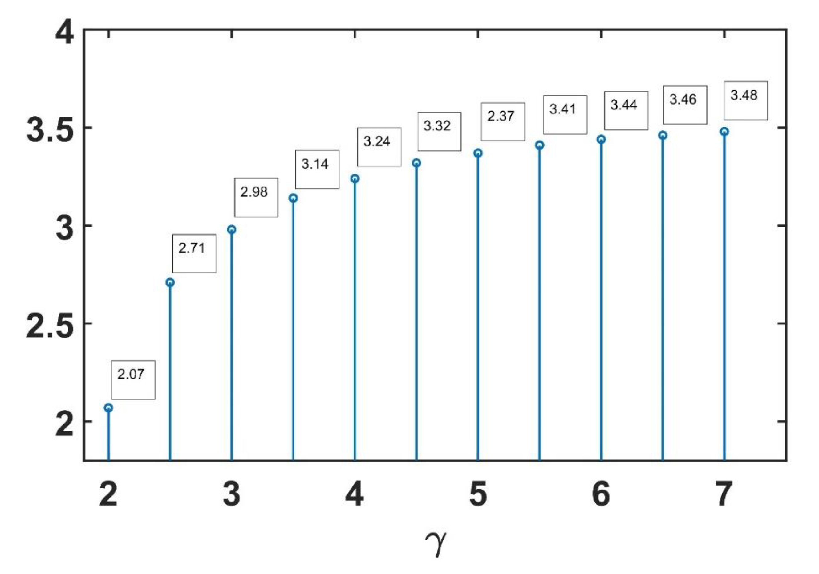
Figure 1.
Maximum for different γ.
3.2. Luenberger State Observer Design
The premise variable is also unavailable which is considered in the paper. Therefore, according to the measurement for (), it is easy to see as follows.
Observer Rule i: IF is and is and … and is
THEN
where is the estimation of the state . is the observer gain having appropriate dimensions to be determined.
In addition, the dynamics of fuzzy observer (14) after fuzzy blending is inferred as
It can be seen from (11) and (13) that . Moreover, the formula of the fuzzy observer is given as follows:
Define as estimated error. Combining (3) with (16), it is easy to obtain:
where is regarded as the disturbance. Obviously, if , then .
Remark 2.
Combined with formulas (16) and (17), it is easy to obtain that the addition of time-delay term makes the effect of sliding mode control better and can better suppress the error.
3.3. Sliding Surface Design
On the basis of (16), we propose a fuzzy integral sliding surface function:
where making nonsingular is chosen, making nonsingular is given. making is Hurwitz is selected.
In view of the systems (16) and (18), as shown as follows
After arriving the sliding surface , i.e., , the equivalent control variable can be obtained as follows:
Then, by substituting (20) into (16), it is easy to obtain:
where and .
Remark 3.
By selecting appropriate such that is invertible. The benefit is that we can obtain the observer gain matrices by solving the optimal problem of the following conditions rather than by given in the design process.
Here, designing a sliding mode controller based on observer for the system (2) is the purpose of this paper and the controller can meet two conditions as follows:
- It is stochastically stable for system (17) with w(t) = 0 and the sliding mode dynamics (21).
- The measurement of H∞ performance with the condition of zero-initial will be satisfied as follows:where is a positive constant.
Remark 4.
By selecting this integral sliding mode functional, the linear LMI is obtained for the obtained sliding mode stochastic stability analysis, so that the gain matrix of the observer can be obtained instead of artificial design, which reduces the conservatism.
3.4. Stochastic Stability and H∞ Performance Analysis
Remark 5.
Given positive scalars , , , and , the error dynamics (17) and the sliding mode dynamics (21) are stochastically stable with an H∞ attenuation level , if matrices , , , , , , free weighting matrices ( = 1, 2, 3) and with appropriate dimensions exist, the following condition is satisfied for each :
The observer gain matrices are computed by .
Proof.
First, the overall closed-loop system is stochastically stable with w(t) = 0 will be proved. Therefore, choose the following stochastic Lyapunov–Krasovskii functional:
It is obvious from the Leibniz–Newton formula that
where , are free weighting matrices. Moreover,
Similarly,
where , are free weighting matrices. Then
On the other hand, it holds that
Then
where and are chosen parameters. In summary, we have
in which
and , where
with
in which
Letting and can be known from (22) by Schur complement. So, if a scaler is denoted, we will know
Hence, after using Dynkin’s formula, some conclusions can be drawn, that is, for
which produces
Then, according to Definition 1, it is stochastically stable when for the sliding mode dynamics (21), and it also can be proved for error system (17) in the same way.
Next, the H∞ performance of overall closed-loop system will be considered. in the condition of zero-initial. Therefore,
in which , and
with
By utilizing Schur’s complement and the inequality (24), obviously, means . Therefore, it is stochastically stable for the sliding mode dynamics (21) with error dynamics (17) with an H∞ disturbance attenuation level . □
Remark 6.
Due to various environmental constraints, the TRs information is often not obtained as expected in practice. Therefore, TRS may encounter three situations, where is completely known, partially known and completely unknown.
For example, the TR matrix may be presented as follows:
in which , and subject to , denote the known values, the estimated values and estimated error of uncertain TRs, respectively. Then “?” denotes TRs that unknown completely. Hereinafter, in order to calculate uniformity, these known TRs are represented by , where , so, the TR matrix can be described further by
where with . According to the above transformation, the following sets are defined:
where
Based on the above sets, the following situations are considered:
- 1.
- andforare known, that isare known, that is;
- 2.
- andforare partially known, that iswhileis also not empty;
- 3.
- andforare partially known, that iswhileis also not empty;
- 4.
- andforare all unknown, that is.
It is known that the above cases 1–3 have been investigated in other works, while the cased 4 was neglected, where is the main difficulty lies. Therefore, in this paper, the following method brought from [48] is introduced.
For the case 4, i.e., and , there exists with is not empty for . In this situation, define
where is the estimated parameter that will be determined.
For example, the three modes TR matrix could be expressed by:
It is seen from the above matrix that is empty, while the unknown TR can be estimated by or . Based on TRs matrix mentioned above, the theorem will be obtained as follows.
Theorem 2.
Given positive scalars , ,, and. The sliding mode dynamics (21) with the error dynamics (17) is stochastically stable with an H∞ attenuation level, if matrices,,,,,,,,free weighting matrices ( = 1, 2, 3) and with appropriate dimensions exist, the following conditions are satisfied for each If and , then
If, there existssuch that, for,
whereis defined as:
and,is defined as:
with
The observer gain matrices are computed by .
Proof.
(Case I): and . □
According to the partition of TRs, letting . Therefore, also is
By using Schur’s complement theory, it seems known that (26) supports Theorem 2 holds in this case.
(Case II): Since , and , while there exists a such that . Here, is estimated by . Denoting .Therefore can be written as
Noting that . For , it satisfies that
In the above formula (30), it has
Then, with the help of Lemma 1 and for any , it can be obtained that
In combination with (28)–(32), by using Schur complement theory, Theorem 2 holds from (27) in this case.
Remark 7.
When analyzing the conditions in Theorem 2, this is an important issue that how to determine . Therefore, proposing the maximum optimization problem to settle this problem, that is
Therefore, the H∞ performance is ensured with unknown TRs.
3.5. Reachability of Sliding Surface
In the section, to guarantee the accessibility of the sliding surface , it will be confirmed that the control scheme proposed will make the estimated state to the pre-designed sliding surface in the limited range of time.
Theorem 3.
Assuming that the conditions in Theorem 2 are solvable and (18) is proposed. By the fuzzy SMC law synthesized as follows, the state trajectories of (16) will be driven onto the sliding surface in the limited range of time:
Proof.
Choose Lyapunov function as follows:
Then
By substituting (33) into (35), we can obtain:
Noting that , then
Now, consider the equation as follows:
where
from 0 to , we integrate both sides it will yield
from this, it is known that a constant exists such that (for all , that is ). In the case where , because of monotonicity, is much smaller. As a result, the reachability is almost guaranteed in the limited range of time. The theorem is completely proved. □
Remark 8.
Compared with the traditional Markov jump system with completely known transfer rate, this study gives a stochastic stability criterion with completely unknown transfer rate of a certain mode, which extends the theoretical depth of this kind of system.
Remark 9.
Theorem 3 not only illustrates the finite time reachability of sliding mode, but also proves the upper bound of the arrival time.
4. Numerical Example
Considering the dynamic equation of the single-link robot arm model as mentioned before
In detail, and , the time invariant . and have three different modes as shown in Table 2. Following the fuzzy approach in Part II, the state-space can be described as follows:
Table 2.
Parameters for and of Different Modes.
Plant Rule 1: IF is “about 0 rad”,
THEN
Plant Rule 2: IF is “about rad or rad”,
THEN
where , and
First, let us check the SMC theory with fully known TR information, and the related TR matrix of the three operation modes is given by:
In this way, we can check the effectiveness of the proposed results based on Theorem 1. Suppose and . In addition, letting the gain matrices , , , , , , and . By solving the condition in (22), it obtains the following feasible solutions:
Therefore, the gain matrices of the observer are computed as
Next, let us consider the case that the TR information is deficient, for instance, the related TR matrix of the three operation modes is given by:
Here, we can estimate by . By selecting , , and the other parameters are chosen as above. After solving the conditions in Theorem 2, it is easy to obtain:
Therefore, the gain matrices of the observer are computed as
Now, let us consider the maximum allowable for feasible solutions of the system with the above parameters by solving the optimal problems in Remark 7. For different H∞ attenuation levels with fixed error tolerance and transmission delay , we can see the maximum allowable for different attenuation levels in Figure 1. From these results, it is easy to obtain that the proposed scheme can reduce the average transmission frequency while maintaining the control performance.
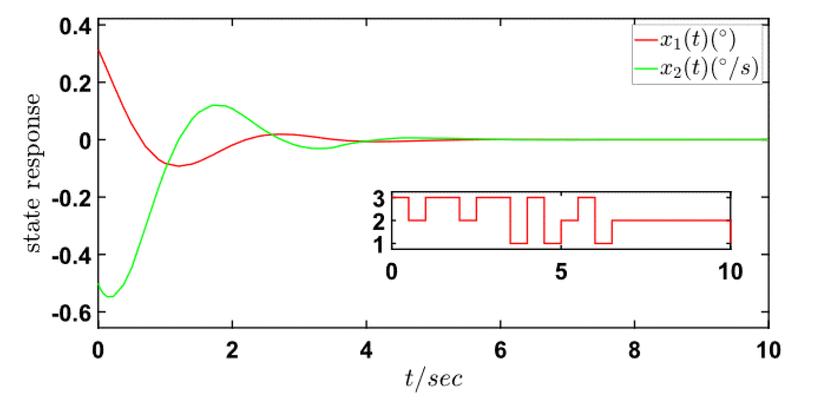
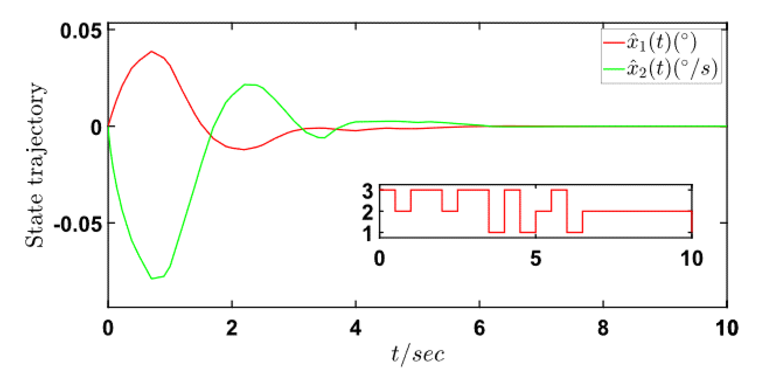
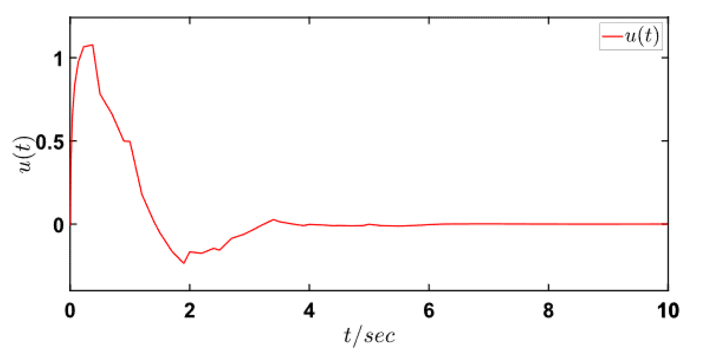
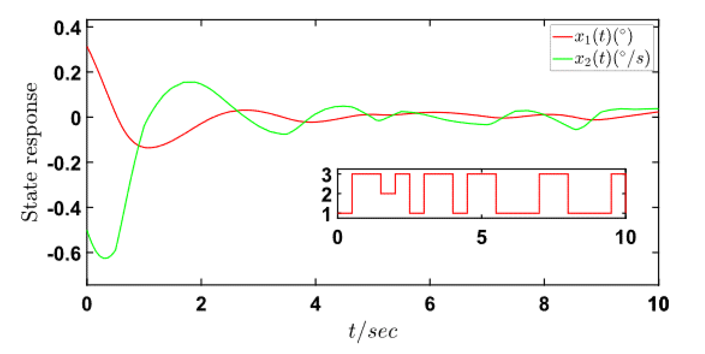
In addition, the state response of the overall closed-loop system with initial conditions and is presented in the following Figure 2, Figure 3 and Figure 4. Figure 2 depicts the state response of original system under control; Figure 3 plots the state response of observer system under control; the controller input is given in Figure 4.
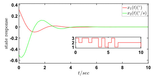
Figure 2.
The state response of original system.
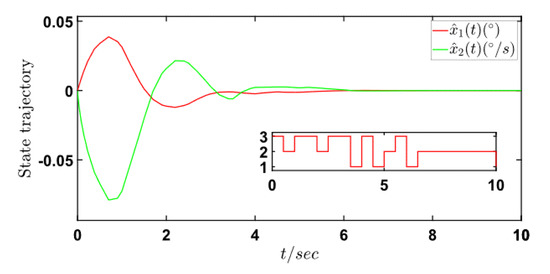
Figure 3.
The state trajectories for the observer system.

Figure 4.
The control input.
Note that although the issue about sliding mode control based on observer for T-S model-based Markovian jump systems has been investigated in this paper, it still leaves much space for improvements. A future study should tackle new problems such as time delay and packet dropout.
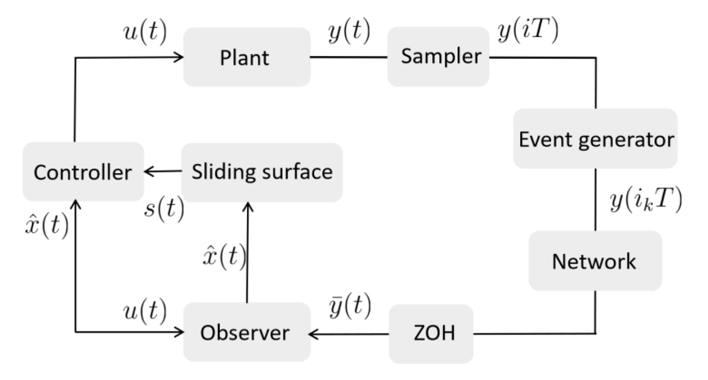
Therefore, the design of state observer in this paper is implemented in the following way: First, select appropriate gain matrices such that is Hurwitz. Second, obtain observer gain matrices by solving the inequalities in Theorem 1 or Theorem 2. Third, set an event-generator based on the parameter obtained in the second step. Last, design the sliding mode controller proposed in (33). The diagram of overall implementation is presented in the following Figure 5.
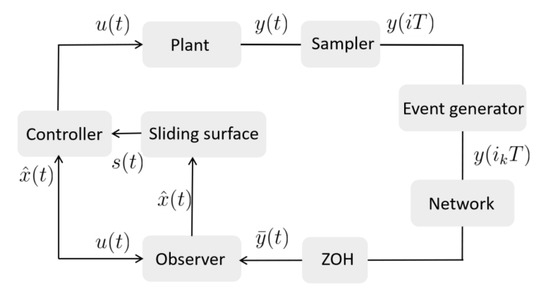
Figure 5.
The diagram of overall closed-loop system.
Finally, in order to verify the advantage of the proposed method, a simulation study is conducted by comparing the system performance on original system based on the state observer without output time-delay, i.e., is changed by . Taking the same parameters above, the simulation result is presented in Figure 6, from which it is seen that, compared with the system performance in Figure 2, much longer time is needed for the system to reach its steady state and the system stability is also affected to some extent. Therefore, proposing a time-delay Luenberger observer is a benefit for the system performance.
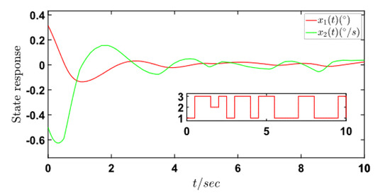
Figure 6.
The state response of original system.
5. Conclusions
In this paper, the issue about sliding mode control based on observer for T-S model-based Markovian jump systems was investigated. Firstly, it involved designing an event-triggered based time-delay sliding mode observer, which can suppress the error and obtain good stability. On this basis, a novel integral sliding surface was proposed and the observer gain matrices can be computed in the design process. Then, according to stochastic stability theory, the H∞ performance of the sliding mode dynamics and the error dynamics were ensured in terms of LMI conditions. In addition, a fuzzy sliding mode controller was constructed to guarantee the finite-time reachability of the predefined sliding surface. Finally, numerical examples based on robotics were presented to verify the effectiveness of the proposed method.
Author Contributions
Conceptualization, C.Z., J.Q. and Z.W.; methodology, M.C., C.Z. and Z.W.; software, M.C., C.Z. and Z.W.; validation, M.C., Z.W. and Q.G.; formal analysis, M.C., J.Q. and Z.W.; investigation, M.C., and Z.W.; resources, M.C., Z.W. and Q.G.; data curation, M.C., C.Z. and J.Q.; writing—original draft preparation, M.C.; writing—review and editing, M.C., J.Q. and Z.W.; visualization, M.C. and C.Z.; supervision, J.Q., Z.W. and Q.G.; project administration, J.Q., Z.W. and Q.G.; funding acquisition, J.Q., Z.W. and Q.G. All authors have read and agreed to the published version of the manuscript.
Funding
This research was funded by Alexander von Humboldt Foundation of Germany: Alexander von Humboldt Foundation of Germany and National Natural Science Foundation of China (No. 61903016).
Institutional Review Board Statement
Not applicable.
Informed Consent Statement
Not applicable.
Data Availability Statement
None.
Conflicts of Interest
The authors declare no conflict of interest.
References
- Krasovskii, N.M.; Lidskii, E.A. Analytical design of controllers in systems with random attributes. Autom. Remote Control 1961, 22, 1021–2025. [Google Scholar]
- Ugrinovskii, V.; Pota, H.R. Decentralized control of power systems via robust control of uncertain Markov jump parameter systems. Int. J. Control 2005, 78, 662–677. [Google Scholar] [CrossRef]
- Andrieu, C.; Davy, M.; Doucet, A. Efficient particle filtering for jump Markov systems. Application to time-varying autoregressions. IEEE Trans. Signal Process. 2003, 51, 1762–1770. [Google Scholar] [CrossRef] [Green Version]
- Wallace, V.L.; Rosenberg, R.S. Markovian models and numerical analysis of computer system behavior. In Proceedings of the Spring Joint Computer Conference, Boston, MA, USA, 26–28 April 1966; pp. 141–148. [Google Scholar] [CrossRef]
- Ellis, R.S. Large deviations for the empirical measure of a Markov chain with an application to the multivariate empirical measure. Ann. Probab. 1988, 16, 1496–1508. [Google Scholar] [CrossRef]
- Souza, C.E.D. Robust stability and stabilization of uncertain discrete-time Markovian jump linear systems. IEEE Trans. Autom. Control 2006, 51, 836–841. [Google Scholar] [CrossRef]
- Gao, H.; Lam, J.; Xu, S.; Wang, C. Stabilization and H∞ control of two-dimensional Markovian jump systems. IMA J. Math. Control Inf. 2004, 21, 377–392. [Google Scholar] [CrossRef]
- Mao, X.; Yuan, C. Stochastic Differential Equations with Markovian Switching; Imperial College Press: London, UK, 2006. [Google Scholar] [CrossRef] [Green Version]
- Wu, L.; Shi, P.; Gao, H.; Wang, C. H∞ filtering for 2D Markovian jump systems. Automatica 2008, 44, 1849–1858. [Google Scholar] [CrossRef]
- Xu, S.; Lam, J.; Mao, X. Delay-dependent H∞ control and filtering for uncertain Markovian jump systems with time-varying delays. IEEE Trans. Circuits Syst. I Regul. Pap. 2007, 54, 2070–2077. [Google Scholar] [CrossRef]
- Fei, Z.; Gao, H.; Shi, P. New results on stabilization of Markovian jump systems with time delay. Automatica 2009, 45, 2300–2306. [Google Scholar] [CrossRef]
- Zhang, L.; Huang, B.; Lam, J. H∞ model reduction of Markovian jump linear systems. Syst. Control Lett. 2003, 50, 103–118. [Google Scholar] [CrossRef]
- Jilkov, V.P.; Li, X.R. Online Bayesian estimation of transition probabilities for Markovian jump systems. IEEE Trans. Signal Process. 2004, 52, 1620–1630. [Google Scholar] [CrossRef]
- Wu, Z.; Su, H.; Chu, J. H∞ filtering for singular Markovian jump systems with time delay. Int. J. Robust Nonlinear Control 2010, 20, 939–957. [Google Scholar] [CrossRef]
- Costa, O.L.V.; Guerra, S. Stationary filter for linear minimum mean square error estimator of discrete-time Markovian jump systems. IEEE Trans. Autom. Control 2002, 47, 1351–1356. [Google Scholar] [CrossRef]
- Takagi, T.; Sugeno, M. Fuzzy identification of systems and its applications to modeling and control. IEEE Trans. Syst. Man Cybern. 1985, SMC-15, 116–132. [Google Scholar] [CrossRef]
- Wang, Y.; Xia, Y.; Shen, H.; Zhou, P. SMC design for robust stabilization of nonlinear Markovian jump singular systems. IEEE Trans. Autom. Control 2018, 63, 219–224. [Google Scholar] [CrossRef]
- Saravanakumar, R.; Ali, M.S.; Karimi, H.R. Robust H∞ control of uncertain stochastic Markovian jump systems with mixed time-varying delays. Int. J. Syst. Sci. 2017, 48, 862–872. [Google Scholar] [CrossRef]
- Park, I.S.; Kwon, N.K.; Park, P. H∞ control for Markovian jump fuzzy systems with partly unknown transition rates and input saturation. J. Frankl. Inst. 2018, 355, 2498–2514. [Google Scholar] [CrossRef]
- Shen, H.; Li, F.; Yan, H.; Karimi, H.R.; Lam, H. Finite-time event-triggered H∞ control for T–S fuzzy Markov jump systems. IEEE Trans. Fuzzy Syst. 2018, 26, 3122–3135. [Google Scholar] [CrossRef] [Green Version]
- Dong, S.; Wu, Z.; Pan, Y.; Su, H.; Liu, Y. Hidden-Markov-model-based asynchronous filter design of nonlinear Markov jump systems in continuous-time domain. IEEE Trans. Cybern. 2019, 49, 2294–2304. [Google Scholar] [CrossRef]
- Zhang, L.; Boukas, E.-K. Stability and stabilization of Markovian jump linear systems with partly unknown transition probabilities. Automatica 2009, 45, 463–468. [Google Scholar] [CrossRef]
- Xiong, L.; Tian, J.; Liu, X. Stability analysis for neutral Markovian jump systems with partially unknown transition probabilities. J. Frankl. Inst. 2012, 349, 2193–2214. [Google Scholar] [CrossRef]
- Kao, Y.; Xie, J.; Wang, C. Stabilization of singular Markovian jump systems with generally uncertain transition rates. IEEE Trans. Autom. Control 2014, 59, 2604–2610. [Google Scholar] [CrossRef]
- Wei, Y.; Qiu, J.; Karimi, H.R. Quantized filtering for continuous-time Markovian jump systems with deficient mode information. Asian J. Control 2015, 17, 1914–1923. [Google Scholar] [CrossRef]
- Liu, M.; Zhang, L.; Shi, P.; Zhao, Y. Sliding mode control of continuous-time Markovian jump systems with digital data transmission. Automatica 2017, 80, 200–209. [Google Scholar] [CrossRef]
- Zhang, H.; Wang, J.; Shi, Y. Robust H∞ sliding-mode control for Markovian jump systems subject to intermittent observations and partially known transition probabilities. Syst. Control Lett. 2013, 62, 1114–1124. [Google Scholar] [CrossRef]
- Song, J.; Niu, Y.; Zou, Y. Asynchronous sliding mode control of Markovian jump systems with time-varying delays and partly accessible mode detection probabilities. Automatica 2018, 93, 33–41. [Google Scholar] [CrossRef]
- Li, H.; Shi, P.; Yao, D.; Wu, L. Observer-based adaptive sliding mode control for nonlinear Markovian jump systems. Automatica 2016, 64, 133–142. [Google Scholar] [CrossRef]
- Liu, M.; Shi, P.; Zhang, L.; Zhao, X. Fault-tolerant control for nonlinear Markovian jump systems via proportional and derivative sliding mode observer technique. IEEE Trans. Circuits Syst. I Regul. Pap. 2011, 58, 2755–2764. [Google Scholar] [CrossRef]
- Jiang, B.; Karimi, H.R.; Yang, S.; Gao, C.; Kao, Y. Observer-based adaptive sliding mode control for nonlinear stochastic Markov jump systems via T–S fuzzy modeling: Applications to robot arm model. IEEE Trans. Ind. Electron. 2021, 68, 466–477. [Google Scholar] [CrossRef]
- Liu, Z.; Yu, J. Non-fragile observer-based adaptive control of uncertain nonlinear stochastic Markovian jump systems via sliding mode technique. Nonlinear Anal. Hybrid Syst. 2020, 38, 100931. [Google Scholar] [CrossRef]
- Karimi, H.R. A sliding mode approach to H∞ synchronization of master-slave time-delay systems with Markovian jumping parameters and nonlinear uncertainties. J. Frankl. Inst. 2012, 349, 1480–1496. [Google Scholar] [CrossRef] [Green Version]
- Zohrabi, N.; Reza Momeni, H.; Hossein Abolmasoumi, A. Sliding mode control of Markovian jump systems with partly unknown transition probabilities. IFAC Proc. Vol. 2013, 46, 947–952. [Google Scholar] [CrossRef]
- Yue, D.; Tian, E.; Han, Q. A delay system method for designing event-triggered controllers of networked control systems. IEEE Trans. Autom. Control 2013, 58, 475–481. [Google Scholar] [CrossRef]
- Su, X.; Liu, X.; Shi, P.; Song, Y.-D. Sliding mode control of hybrid switched systems via an event-triggered mechanism. Automatica 2018, 90, 294–303. [Google Scholar] [CrossRef]
- Peng, C.; Han, Q.; Yue, D. To transmit or not to transmit: A discrete event-triggered communication scheme for networked Takagi–Sugeno fuzzy systems. IEEE Trans. Fuzzy Syst. 2013, 21, 164–170. [Google Scholar] [CrossRef]
- Behera, A.K.; Bandyopadhyay, B.; Yu, X. Periodic event-triggered sliding mode control. Automatica 2018, 96, 61–72. [Google Scholar] [CrossRef]
- Dimarogonas, D.V.; Frazzoli, E.; Johansson, K.H. Distributed event-triggered control for multi-agent systems. IEEE Trans. Autom. Control 2012, 57, 1291–1297. [Google Scholar] [CrossRef]
- Cheng, J.; Park, J.H.; Zhang, L.; Zhu, Y. An asynchronous operation approach to event-triggered control for fuzzy Markovian jump systems with general switching policies. IEEE Trans. Fuzzy Syst. 2018, 26, 6–18. [Google Scholar] [CrossRef]
- Wang, L.; Wang, Z.; Wei, G.; Alsaadi, F.E. Finite-time state estimation for recurrent delayed neural networks with component-based event-triggering protocol. IEEE Trans. Neural Netw. Learn. Syst. 2018, 29, 1046–1057. [Google Scholar] [CrossRef] [PubMed]
- Wu, L.; Gao, Y.; Liu, J.; Li, H. Event-triggered sliding mode control of stochastic systems via output feedback. Automatica 2017, 82, 79–92. [Google Scholar] [CrossRef]
- Huai-Ning, W.; Kai-Yuan, C. Mode-independent robust stabilization for uncertain Markovian jump nonlinear systems via fuzzy control. IEEE Trans. Syst. Man Cybern. Part B 2006, 36, 509–519. [Google Scholar] [CrossRef] [PubMed]
- Tanaka, K.; Kosaki, T. Design of a stable fuzzy controller for an articulated vehicle. IEEE Trans. Syst. Man Cybern. Part B 1997, 27, 552–558. [Google Scholar] [CrossRef] [PubMed]
- Meyn, S.P.; Tweedie, R.L. Markov Chains and Stochastic Stability; Springer Science & Business Media: Berlin/Heidelberg, Germany, 2012. [Google Scholar]
- Boukas, K. Stabilization of stochastic nonlinear hybrid systems. Int. J. Innov. Comput. Inf. Control 2005, 1, 131–141. [Google Scholar] [CrossRef]
- Xiong, J.; Lam, J. Robust H2 control of Markovian jump systems with uncertain switching probabilities. Int. J. Syst. Sci. 2009, 40, 255–265. [Google Scholar] [CrossRef] [Green Version]
- Jiang, B.; Gao, C. Decentralized adaptive sliding mode control of large-scale semi-Markovian jump interconnected systems with dead-zone input. IEEE Trans. Autom. Control 2021. [Google Scholar] [CrossRef]
Publisher’s Note: MDPI stays neutral with regard to jurisdictional claims in published maps and institutional affiliations. |
© 2021 by the authors. Licensee MDPI, Basel, Switzerland. This article is an open access article distributed under the terms and conditions of the Creative Commons Attribution (CC BY) license (https://creativecommons.org/licenses/by/4.0/).