Abstract
Conclusive evidence has demonstrated the critical importance of adaptive cruise control (ACC) in relieving traffic congestion. To improve the performance of the ACC system, this paper proposes a novel ACC strategy for electric vehicles based on a hierarchical framework. Three main efforts have been made to distinguish our work from the existing research. Firstly, a sliding acceleration identification model is established based on the recursive least squares algorithm with multiple forgetting factors (MFF-RLS). Secondly, with vehicle following, economy, and comfort as the optimization objectives, the upper-level controller is developed based on the model predictive control (MPC) algorithm. Benefit from the identification of the sliding acceleration, the MPC controller holds better capability in accommodating environmental changes. Thirdly, an iterative learning lower-level controller is designed to control the driving and braking systems. Considering the efficiency of regenerative braking, the braking force distribution strategy is also designed in the lower-level controller. Simulation results show that, compared with the conventional MPC-based ACC strategy, the proposed strategy has similar performance in vehicle following, but it makes great improvements in comfort and economy. The specific features are that the vehicle acceleration and speed fluctuation are significantly reduced, and the energy consumption is also reduced by 2.05%.
1. Introduction
In recent years, the rapid development of the economy has resulted in a great increase in car ownership, leading to a series of social problems such as environmental pollution, traffic congestion, and traffic accidents [1,2]. Advanced driver assistance systems (ADAS) are regarded as an effective solution to these problems because of their great potential in reducing energy consumption, improving vehicle safety, and increasing road capacity [3,4]. As a representative application of ADAS, the adaptive cruise control (ACC) system has been widely used in passenger vehicles. By automatically adjusting the throttle and brake, the ACC system can keep a safe vehicle space from the preceding vehicle, which is beneficial both in terms of saving energy and in reducing the collision risk caused by driver fatigue [5,6,7,8].
The performance of the ACC system is mainly determined by the design of the ACC controller. Currently, safe car-following is the most important issue in the design of the ACC controller. Meanwhile, many manufacturers are also considering how to improve comfort and economy on the premise of ensuring safe car-following [9,10,11]. As safe car-following, comfort, and economy usually conflict with each other, coordinating them simultaneously creates great challenges for designers. Additionally, a well-designed ACC controller should not only satisfy the control objectives and constraints but also perform robustly under system disturbances and model mismatches. Nowadays, many researchers have been working on designing ACC controllers based on different control algorithms, such as the optimal control algorithm [12], fuzzy control algorithm [13], sliding mode control algorithm [14], neural network learning algorithm [15], proportional–integral–derivative (PID) control algorithm [16], and the model predictive control (MPC) algorithm [17,18,19,20,21,22,23,24,25,26,27,28,29].
Among the above control algorithms, MPC is a closed-loop control algorithm that can predict the future state of the ACC system. Based on the future state information, MPC can easily realize closed-loop optimization of multiple control objectives under specific constraints, so as to reduce the control error caused by system disturbances and model mismatches [17,18,19]. Therefore, MPC has received a great deal of attention for automotive control applications. For instance, Bageshwar et al. designed an ACC controller based on MPC, which considered distance error and speed error in the cost function, and the constraint was built by limiting the vehicle longitudinal acceleration [20]. Li et al. adopted MPC theory in designing a multi-objective ACC controller. Car-following, fuel economy and the driver desired response were considered in the cost function. To avoid the unfeasible solution, the constraint softening method was employed [21]. Kohut et al. presented an MPC-based headway control algorithm to balance trip time and fuel consumption while following the preceding vehicle [22]. Yu et al. used MPC to maintain safe vehicle spacing from the lead vehicle. To optimize the vehicle speed trajectory, intelligent transportation systems(ITS) and road slope information were introduced into the controller [23]. Sun et al. designed an ACC controller based on the MPC theory with a particle swarm optimization algorithm. With braking energy, tracking, comfort, and safety as the control objectives, the vehicle could recover braking energy as much as possible while satisfying the requirements of tracking, safety, and comfort [24]. Sakhdari and Nasser L proposed an adaptive tube-based nonlinear model predictive control (AT-NMPC) method to design the ACC system. The proposed method contained two separate models, one for dealing with the problem constraints and the other for defining the objective function [25]. Zhang et al. designed a multi-objective coordinated ACC controller based on an MPC framework, which could simultaneously handle issues regarding vehicle safety, lateral stability, and longitudinal tracking performance. To improve the overall tracking performance, a weight coefficient self-tuning strategy was introduced into the MPC controller so that the weight coefficients could be adjusted automatically with the change of traffic scenarios [26]. Nie and Farzaneh developed an eco-driving ACC system for two typical car-following traffic scenes. The ACC system was designed using the MPC algorithm, which took driving safety, eco-driving, tracking capability, and comfort as the control objectives [27]. Li et al. presented an MPC-based ACC controller, which considered the nonlinear powertrain dynamics, road elevation information, and spatiotemporal constraint from the preceding vehicle [28]. Ma et al. used MPC to develop the CACC system for an electric vehicle platoon. To efficiently solve the problem of the discrete variables, a simulated annealing-particle swarm optimization (SA-PSO) algorithm was employed [29].
Most of the above research does not take the switching performance between driving and braking into consideration. In the design of the ACC controller, the driving and braking state of the ACC system is usually determined by the relationship between the sliding acceleration (acceleration when the vehicle is neither driving nor braking) and the desired acceleration. If the desired acceleration is greater than the sliding acceleration, the vehicle will enter driving mode, otherwise, it will enter braking mode [30,31,32]. In real traffic systems, the vehicles are always accompanied by disturbances such as wind and road slope, which greatly affect the driving resistance, as well as the sliding acceleration. As the vehicle cannot measure the sliding acceleration in real-time, the ACC system usually presets a sliding acceleration. When the preset sliding acceleration is close to the actual value, the ACC system can accurately determine the driving or braking mode it should be in, which will not make negative impacts on the ACC performance. However, when the preset sliding acceleration deviates from the actual value and the desired acceleration is near the actual value, it is difficult for the ACC system to determine whether to drive or to brake. Once the mode is judged wrong, the control error caused by model mismatches will increase significantly. To reduce the error, the ACC system will frequently switch between driving and braking for feedback correction, which will lead to mechanical damage of vehicle components, the loss of energy, fluctuations of the vehicle dynamics, discomfort, and dissatisfaction from passengers [33].
As the switching performance between driving and braking is critical to the vehicle’s comfort and economy, a novel ACC strategy that considers the switching performance is proposed in this paper. Compared with the current work, the main contributions of this paper are as follows:
- (1)
- A sliding acceleration identification model based on the recursive least squares algorithm with multiple forgetting factors (MFF-RLS) is established in the ACC system;
- (2)
- With vehicle following, economy, and comfort as the optimization objectives, the MPC upper-level controller is designed in the ACC system. Considering the influence of switching performance on economy and comfort, the identified sliding acceleration is introduced into the MPC controller and the switching performance is optimized.
- (3)
- An iterative learning lower-level controller is designed to control the driving and braking systems. To improve the efficiency of regenerative braking, the braking force distribution strategy is also designed in the lower-level controller.
The remainder of this paper is organized as follows. Section 2 describes the vehicle platform and the control framework. Section 3 presents the sliding acceleration identification model. Section 4 presents the MPC-based multi-objective ACC strategy with constraints. Section 5 explains the lower-level controller with the braking force distribution strategy. Simulation results and analysis are discussed in Section 6. Lastly, conclusions are drawn in Section 7.
2. Vehicle Platform and Control Framework
2.1. Vehicle Platform
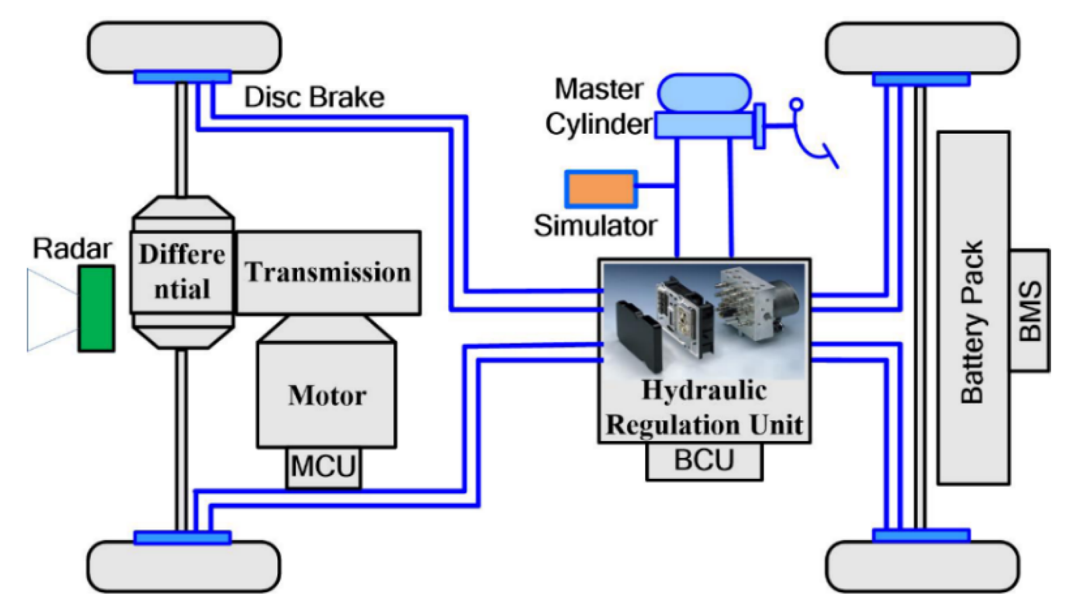
As shown in Figure 1, the ACC system proposed in this paper is deployed on a front-wheel-drive electric vehicle. The vehicle is equipped with radars to detect the moving obstacles ahead. A permanent magnet synchronous motor with a motor control unit (MCU) is used to drive the vehicle through the transmission and differential. To provide energy for the motor and store the recovered braking energy, the vehicle is equipped with a high-voltage battery pack and battery management system (BMS). There is a disc brake on each wheel of the vehicle. The pressure in the brake comes from the hydraulic regulation unit, which is controlled by a brake control unit (BCU). When the ACC system works, the ACC controller calculates the vehicle’s accelerating and braking demands in real-time based on the environmental information from the radars. The MCU and BCU receive the corresponding commands from the ACC system and control the actuators to execute.
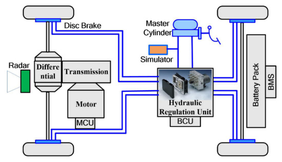
Figure 1.
Structure of the electric vehicle.
2.2. Control Framework
The fundamental function of the ACC system is to automatically regulate the host vehicle speed to maintain safe vehicle spacing from the lead vehicle. As shown in Figure 2, the control framework of the ACC system is designed to be hierarchical. In the upper-level controller, a sliding acceleration identification model is firstly established based on MFF-RLS. Then the identified sliding acceleration is introduced into the MPC controller. With vehicle following, economy, and comfort as the optimization objectives, the desired acceleration is calculated. In the lower-level controller, the mode switching logic is designed first to determine the operating mode of the host vehicle (braking or driving). Then, the torque and pressure demands for driving and braking are calculated and sent to the vehicle model so that the host vehicle can accurately track the desired acceleration.
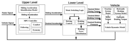
Figure 2.
Control framework of the ACC system.
The vehicle model is established by Matlab/Simulink, which consists of a traction system model, a hydraulic braking system model, and a vehicle dynamics model. The traction system model contains the motor, battery, MCU, and BMS models, which accept the desired motor torque and output the actual motor torque. The hydraulic braking system model contains the master cylinder, pedal simulator, hydraulic regulation unit, disc brakes, and BCU models, which control the solenoid valves in the hydraulic regulation unit according to the desired pressure and output the hydraulic braking torque. The vehicle dynamics model contains the wheel, suspension, and spring-loaded mass models, which accept the actual motor torque and hydraulic braking torque, and feeds the vehicle status to the upper and lower level controller. The specific modeling process of the vehicle model can be found in [34], which will not be discussed here.
3. Sliding Acceleration Identification Model
For mode switching optimization, the key point is to obtain the sliding acceleration of the host vehicle. During the normal driving process, since the vehicle driving system and braking system need to work in real-time, the vehicle can’t enter the sliding state to acquire the sliding acceleration directly, so it’s necessary to identify the sliding acceleration by other methods. At present, there is little research on the identification of sliding acceleration. Li SB et al. obtained the speed-sliding acceleration curve through the vehicle coast-down test and used it as the mode switching threshold [35,36]. Tsai et al. ignored the test calibration and took zero as the sliding acceleration [37]. Kim et al. constructed a linear function with constant parameters to fit the relationship between vehicle speed and sliding acceleration [38]. Through theoretical analysis of vehicle longitudinal dynamics, Li et al. derived a formula of vehicle speed and sliding acceleration [39].
The above studies all obtained the speed-sliding acceleration relationship by one offline calculation, which neglected the effect of external drag changes on the sliding acceleration. Therefore, this section proposes an online sliding acceleration identification model. Firstly, the sliding acceleration identification model is established according to the vehicle driving equation. Then, based on the vehicle CAN information, the equivalent sliding acceleration is calculated. Finally, the unknown parameters in the sliding acceleration identification model are estimated by the MFF-RLS algorithm.
3.1. Modeling of the Sliding Acceleration
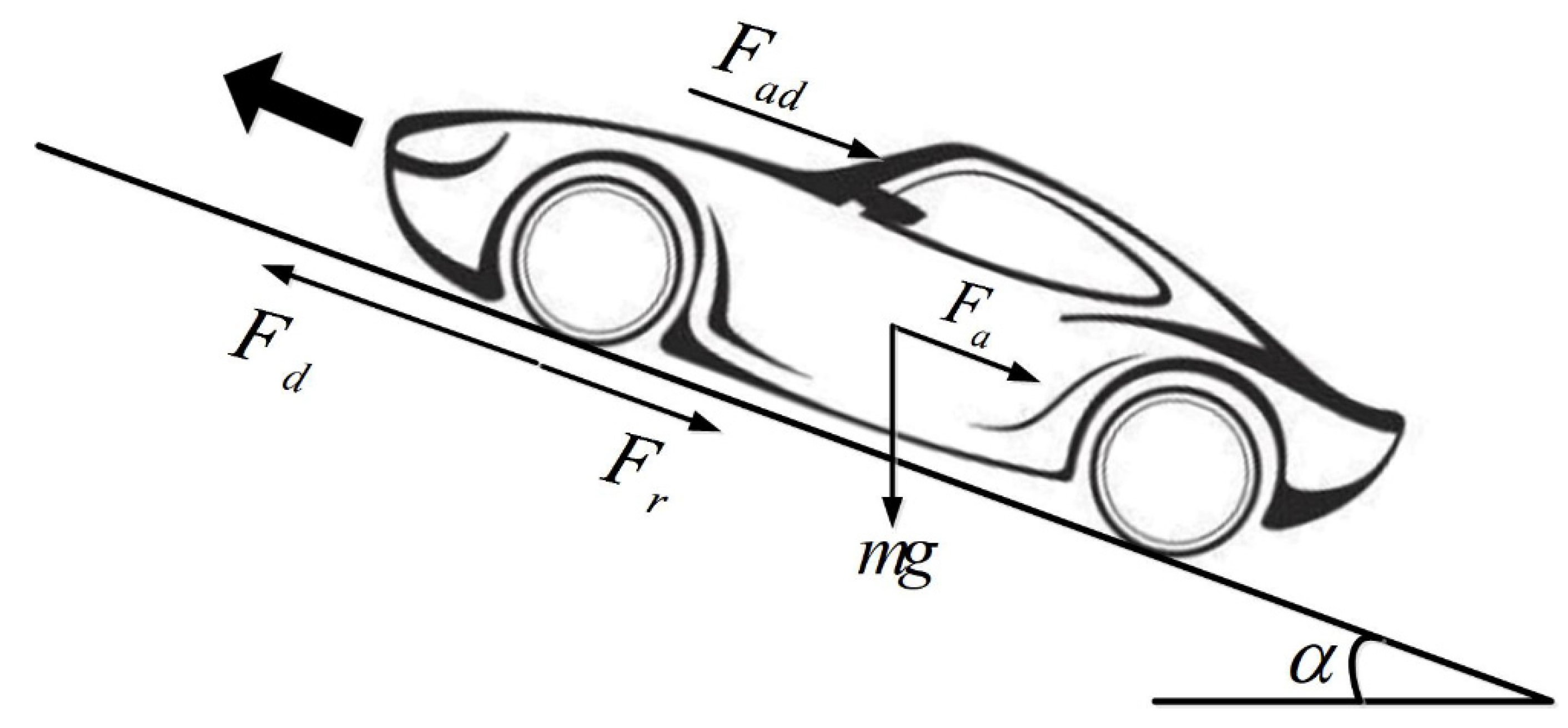
As shown in Figure 3, the resistance of the host vehicle in the driving direction mainly includes four parts: rolling resistance, aerodynamic drag, accelerating resistance, and slope resistance caused by gravity.

Figure 3.
Vehicle longitudinal forces on slope.
To overcome the above resistance, the motor generates the driving force acting on the wheel. The equation of driving force and running resistance of the host vehicle is listed as follows:
where is the driving force, is the rolling resistance, is the aerodynamic drag, is the slope resistance, is the accelerating resistance, is the vehicle mass, is the rolling resistance coefficient, is the gravity acceleration, is the road slope, is the mass density of air, is the aerodynamic drag coefficient, is the vehicle frontal area, is the host vehicle speed, is the wind speed, is the correction coefficient of rotating mass, is the host vehicle acceleration.
When the host vehicle is in the sliding state, neither the driving system nor the braking system is in operation. At this time, the vehicle is only subject to rolling resistance, aerodynamic drag, slope resistance and accelerating resistance. The vehicle sliding acceleration can be expressed as follows:
where is the vehicle sliding acceleration.
If we modify Formula (2), a mathematical model of the sliding acceleration can be established as shown in Formula (3).
It can be seen that A is the quadratic coefficient, which is related to vehicle design parameters; B is the primary coefficient, which is related to wind speed and vehicle design parameters; C is a constant term, which is related to vehicle design parameters, wind speed, and road conditions. Therefore, for a specific vehicle, A is a constant value, and B and C are time-varying values. If we could estimate the B and C coefficients in real-time, the sliding acceleration at any speed could be identified.
3.2. Calculation of Equivalent Sliding Acceleration
According to Formula (3), the estimation of parameters B and C requires real-time sliding acceleration data, which cannot be acquired directly. Therefore, the equivalent sliding acceleration is used instead of the actual sliding acceleration data for parameter estimation.
By observing and recording the CAN bus information, we can get the vehicle speed , vehicle acceleration , motor driving torque , motor braking torque , cylinder pressure of front and rear axle , at k moment.
According to the balance equation of vehicle driving force and driving resistance, the equivalent sliding acceleration of the driving process can be obtained as follows:
where is the equivalent sliding acceleration of the driving process, is the vehicle acceleration generated by driving force, is the vehicle transmission ratio, is the transmission efficiency, is the wheel radius.
According to the balance equation of vehicle braking force and driving resistance, the equivalent sliding acceleration of the braking process can be obtained as follows:
where is the equivalent sliding acceleration of the braking process, is the vehicle deceleration generated by braking force, , are the cylinder diameters of the front and rear wheel, , are the effective radiuses of the front and rear wheel, , are the braking efficiency factors of the front and rear wheel.
Through equivalent treatment, the equivalent sliding acceleration of the driving and braking process can be unified as the equivalent sliding acceleration . According to Formulas (4) and (5), the equivalent sliding acceleration is the difference between vehicle actual acceleration and the vehicle acceleration generated by driving or braking force. Since is obtained considering the effect of vehicle driving and braking system, it is close to the actual sliding acceleration, but with more dramatic fluctuations.
Due to the great fluctuations, the equivalent sliding acceleration cannot directly replace the actual sliding acceleration for ACC control, but it can be used for the estimation of unknown parameters. After estimating parameters B and C, the sliding acceleration can be calculated indirectly.
By replacing the vehicle actual sliding acceleration with the equivalent sliding acceleration, Formula (3) can be transformed into Formula (6).
In Formula (6), the equivalent sliding acceleration can be calculated from vehicle acceleration, motor torque, and braking pressure, the vehicle speed can be obtained from CAN bus, the parameter A is a constant value, so the only unknown parameters in Formula (6) are parameters B and C. As long as there are two sets of sampled data, the unknown parameters B and C can be estimated. The detailed estimating process of parameters B and C is described as follows.
3.3. Recursive Least Squares Algorithm with Multiple Forgetting Factors
After obtaining the equivalent sliding acceleration, we need to use experimental data to modify the mathematical model. By constructing the error function between model results and actual results, we can continuously estimate the unknown parameters B and C in the mathematical model with the objective of minimizing the error function. At present, the classical algorithms of parameter estimation mainly include the least-squares algorithm [40] and the maximum likelihood algorithm [41]. With the development of optimization theory, some intelligent optimization algorithms which simulate and reveal natural phenomena and processes, such as genetic algorithm [42], particle swarm optimization algorithm [43], and ant colony algorithm [44] have been widely used because of their unique characteristics in parameter estimation of non-linear systems. But the computational complexity of these intelligent optimization algorithms is too large to satisfy the function of online real-time identification.
Now, the most widely used algorithm in parameter estimation is the recursive least squares (RLS) algorithm [45]. However, the traditional RLS algorithm is more suitable for the system with constant parameters, when it comes to the system with time-varying parameters, the traditional RLS algorithm may not work well [46]. In this paper, the parameters to be estimated are affected by the change of wind speed and road slope. In order to avoid the failure of parameter identification, we could increase the weight of the latest observation data and reduce the weight of the previous observation data. In other words, we can introduce the forgetting factor to solve the problem. Because there are two parameters to be estimated in this paper, we select the corresponding forgetting factors for both estimated parameters and propose the recursive least square algorithm with multiple forgetting factors (MFF-RLS).
Transform Formula (6) into the form of RLS requirements, namely:
where , , represent the measured value, coefficient matrix, the system parameter at k moment respectively.
According to the basic idea of the least-squares algorithm, we select the residual sum of squares between the measured value and the estimated value to establish the fitness function as follows:
where and represent forgetting factors for estimated parameters and respectively.
In order to determine the estimated parameter and minimize the fitness function value, set and , then the estimated parameter can be obtained as:
To realize real-time parameter estimation, Formula (9) should be converted into the recursive form shown in Formulas (10) and (11).
where, are the gain matrix, are the covariance matrix.
In addition, because and are unknown in Formulas (10) and (11), the estimated values and are used instead, it can be obtained that:
4. MPC Controller Design
The upper-level ACC controller based on MPC is designed in this section. Firstly, the vehicle predictive model is established according to the vehicle longitudinal kinematic characteristics. Then, with vehicle following, economy, and comfort as the optimization objectives, the objective function for the ACC system is developed. Finally, the system constraints for speed error, distance error, and acceleration are introduced into the MPC controller.
4.1. Vehicle Predictive Model
The current control input of MPC is obtained by solving the optimal control problem in the prediction time domain, which requires high computational efficiency. In order to simplify the calculation, assuming that the lead vehicle can maintain a uniform acceleration at k moment, then the predictive model of the lead vehicle can be expressed as:
where , , are respectively the driving distance, speed and acceleration of the lead vehicle; is the sampling time.
For the host vehicle, since the vehicle driving system has delay characteristics, the relationship between the desired acceleration and the actual acceleration can be described by the first-order inertia link.
where is the time lag of the vehicle driving system, is the desired acceleration output by the MPC controller.
Using the differential approximation method, Formula (14) can be transformed into the discretized format as follows:
Combined with the vehicle longitudinal kinematic characteristics, the predictive model of the host vehicle can be established as follows:
where is the driving distance of the host vehicle.
Combining the lead and host vehicle predictive models, the integrated vehicle predictive model can be defined as
Choose the driving distance of the lead vehicle , the speed of the lead vehicle , the acceleration of the lead vehicle , the driving distance of the host vehicle , the speed of the host vehicle , and the acceleration of the host vehicle as the state variables, that is . Choose the desired acceleration of the host vehicle as the control input, that is . Then, the integrated predictive model can be transformed into the form of state space equation as follows:
Selecting the prediction time domain as P, the state variable at each moment under the prediction time domain can be expressed as
Since the initial state of the ACC system is known, the state at next moment can be predicted according to the Formula (18). Based on the prediction results, the optimal control can be carried out. According to Formula (19), the prediction process can run continuously, and the state information at any time in the prediction time domain can be obtained.
4.2. Objective Function
The objective function of the proposed ACC system includes three indexes: the following performance index, the comfort performance index, and the economy index.
It is accepted that the following performance of the ACC system includes speed following and distance following. Therefore, speed error and distance error are considered in the calculation of the following index, which is shown as follows:
where is the following performance index, is the weight coefficient of distance error, is the distance error, is the weight coefficient of speed error, is the speed error, is the desired inter-vehicle distance.
With respect to , the desired inter-vehicle distance is affected by driver preference, road commuting efficiency, and vehicle safety. If the vehicle spacing is too narrow, the commuting efficiency will improve, but the anxiety of the driver may lead to crashes. On the contrary, a large vehicle spacing is the guarantee of vehicle safety, but the road commuting efficiency will get worse and the side lane vehicles can easily insert. Nowadays, the constant time headway (CTH) [47] is commonly used in vehicle spacing algorithm, which is shown as follows:
where is the nominal time headway, is the safe stopping distance.
As frequent mode (driving or braking) switching and unreasonable longitudinal acceleration make negative impacts on driver feeling and vehicle economy, the comfort and economy of the ACC system can be improved via penalizing acceleration and mode switching frequency.
For the mode switching frequency, assuming that B and C coefficients in Formula (6) remain unchanged in the prediction time domain, the ACC operating mode can be expressed by Formula (22).
where is the ACC operating mode, 1 represents driving mode and 0 represents braking mode.
According to Formula (22), the less jumps between 0 and 1, the smaller the mode switching frequency. Therefore, the mode switching frequency of the ACC system can be expressed as
where is the mode switching frequency of ACC system.
Combining the mode switching frequency and the square of the acceleration, the combined comfort and economy index of the ACC system can be expressed as
where is the combined comfort and economy index, is the weight coefficient of mode switching frequency, is the weight coefficient of acceleration.
According to Formula (20) and Formula (24), the objective function can be expressed as
4.3. System Constraints
Considering the vehicle physical limitations as well as the driver-permissible following error range, the maximum and minimum values of the state variables and control commands are constrained as follows
Organizing the above objective function and constraint, the optimization problem can be transformed into the following form
where
The objective function is a nonlinear discontinuous function, the interior point method can be used to solve this nonlinear programming problem [48].
5. Lower-Level Controller
The objectives of the lower-level controller are controlling the driving and braking systems so that the vehicle acceleration can steadily follow the desired acceleration. Since the driving and braking systems are two different systems that cannot work simultaneously, the lower-level controller should firstly determine the operating mode of the vehicle. In this paper, the driving and braking modes are determined based on the desired acceleration and the identified sliding acceleration. When the desired acceleration is greater than the sliding acceleration, the vehicle will enter the driving mode; when the desired acceleration is less than the sliding acceleration, the vehicle will enter the braking mode.
For the control of driving and braking torque, the iterative learning algorithm is used in this paper. As a control algorithm with self-learning ability, the iterative learning algorithm does not need the exact model of the system itself, and has strong adaptability to the nonlinear system and time-varying system. The principle of the iterative learning algorithm is to use the system input of the previous cycle and the tracking error of the current cycle to modify the system input of the current cycle so that the system output can gradually converge to the desired output. In addition, the iterative learning algorithm belongs to the feedforward control algorithm, its key lies in the design of the updating law. Currently, the commonly used updating law includes P-type, PI-type, PD-type, and PID-type [49]. Considering that the vehicle dynamics model has certain hysteresis, the PD-type updating law is adopted to design the lower-level controller as follows:
where, is the system input, is the tracking error, and represent the learning gain factors of proportional and differential parts respectively, is the number of iterations.
In detail, when the mode switching logic determines that the vehicle should enter the driving mode, the desired acceleration will be modified by the ACC driving controller. The design of the driving controller is as follows:
where, is the modified acceleration output to the vehicle driving system at nth iteration. To compensate for the disturbance of external driving resistance, the initial iteration value is set as the sliding acceleration identified by the MFF-RLS algorithm.
The modified driving acceleration obtained by the iterative learning algorithm needs to be converted into the motor driving torque requirements, which can be calculated by Formula (31):
where, is the required motor driving torque at nth iteration.
If the mode switching logic determines that the vehicle should enter the braking mode, the ACC braking controller will modify the desired acceleration. The braking controller of the ACC system is designed as follows:
where, is the modified acceleration output to the vehicle braking system at nth iteration.
Convert the modified braking acceleration into the braking torque requirements, namely:
where, is the required braking torque at nth iteration.
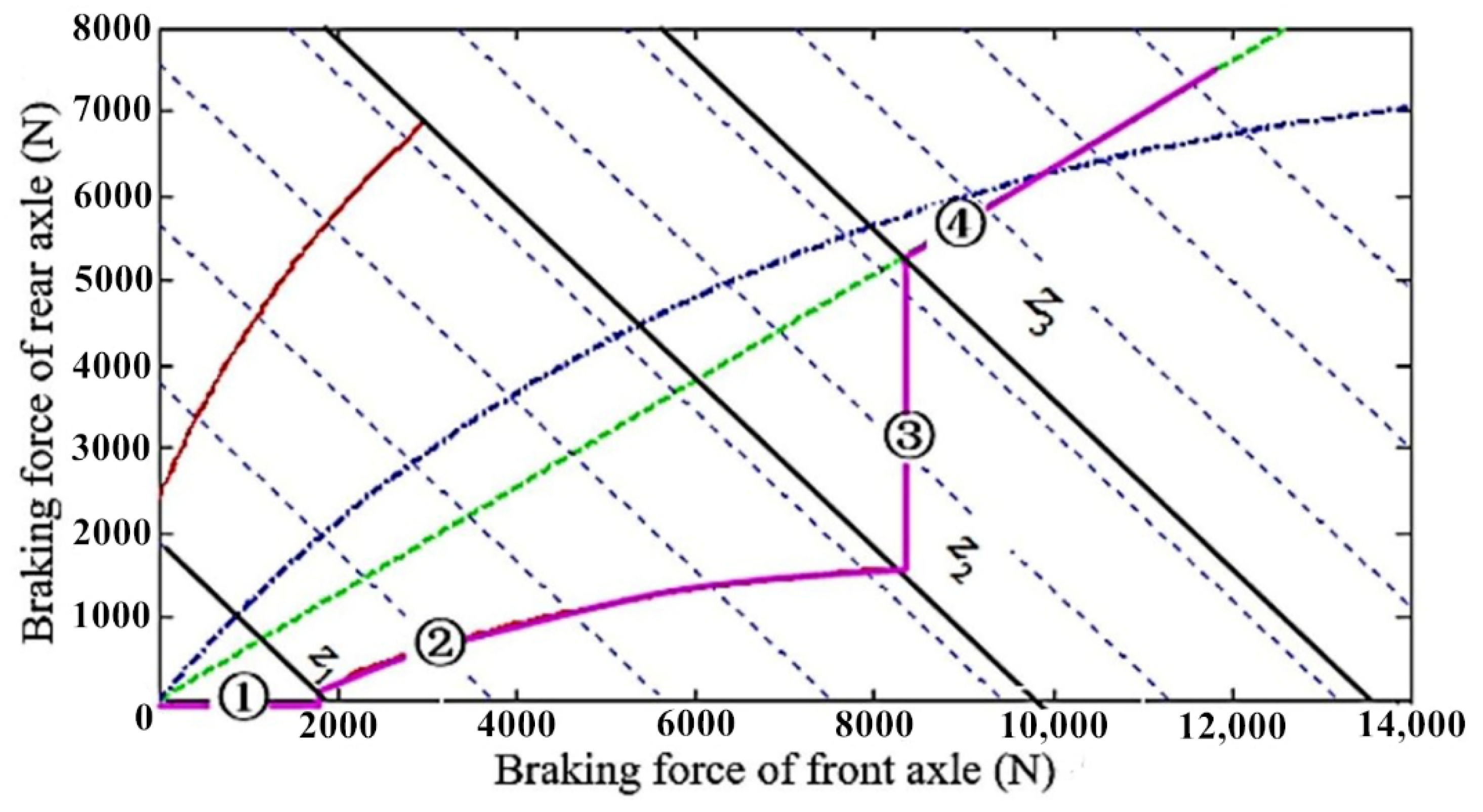
As the electric vehicle has regenerative braking function, the required braking torque needs to be distributed into motor braking torque and hydraulic braking torque according to the braking force distribution strategy. The key point of the braking force distribution strategy is to recycle as much energy as possible while ensuring braking safety. In this paper, the target vehicle is driven by the front axle, so the braking force distribution strategy should distribute more force to the front axle.
Considering the restriction of braking force distribution by ECE regulations, this paper designs the braking force distribution strategy as shown in Figure 4. When the braking strength , the braking force is provided by the front axle only; when the braking strength , the braking force of front and rear axle is distributed along the ECE regulation line; when the braking strength , the braking force of the front axle keeps unchanged and the braking force of the rear axle increases; when the braking strength , the motor braking is stopped, the braking force of front and rear axle is distributed along the line. In the whole braking process, if the motor braking force is insufficient, the hydraulic braking force will compensate for the loss of total braking force. The braking force distribution can be expressed as follows:
| (34) | |
| (35) | |
| (36) | |
| (37) |

Figure 4.
Braking force distribution strategy.
The boundary condition is calculated as follows:
where is the braking force of the front axle, is the braking force of the rear axle, is the total demand force, is the total wheelbase, is the rear wheelbase, is the height of mass center, is the maximum value of motor braking torque, is the brake force distribution coefficient.
In the above controller design process, the selection of the learning gain factors determines the convergence speed and control error of the iterative learning control algorithm. To improve the running efficiency of the ACC system, the iterative learning algorithm uses fixed learning gain factors. When the vehicle is in the driving mode, set ; When the vehicle is in the braking mode, set .
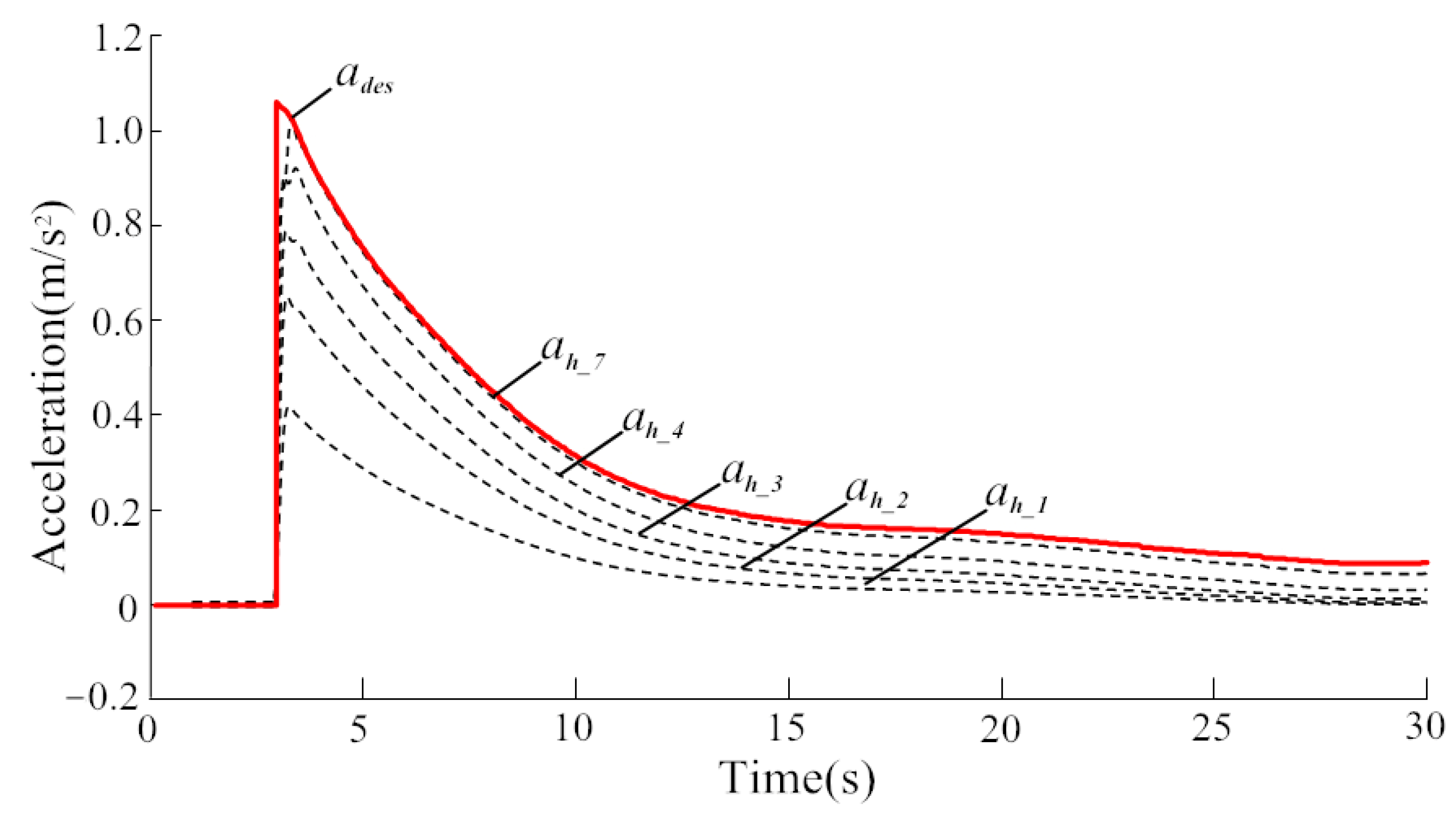
Figure 5 and Figure 6 show the actual acceleration and desired acceleration curves of the vehicle during driving and braking processes. It can be seen that the control error gradually decreases as the number of iterations increases. After seven iterations, the actual acceleration curve fits the desired acceleration curve almost exactly, showing the effectiveness of learning gain factor selection.

Figure 5.
Actual and desired acceleration during the driving process.
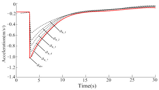
Figure 6.
Actual and desired acceleration during the braking process.
6. Simulation Results and Analysis
To verify the effectiveness of the proposed ACC strategy, several experiments are conducted utilizing Matlab/Simulink. The main parameters used in the simulations are set in Table 1.

Table 1.
Main parameters used in the simulations.
6.1. Simulation and Analysis of the Sliding Acceleration Identification Model
According to Formula (3), the sliding acceleration is mainly affected by the wind speed and road slope. Therefore, we select wind speed and road slope change conditions to verify the effectiveness of the sliding acceleration identification model.
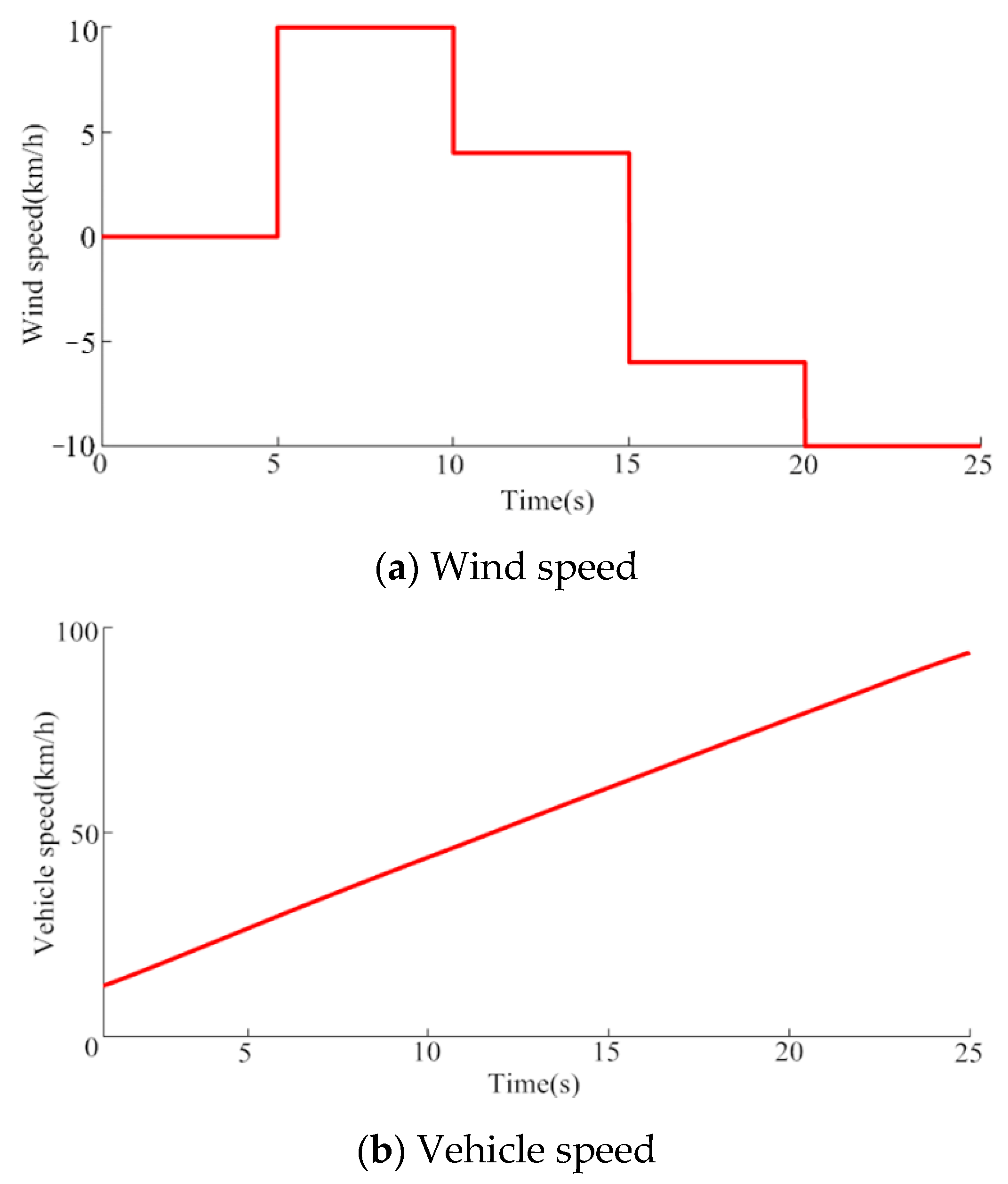
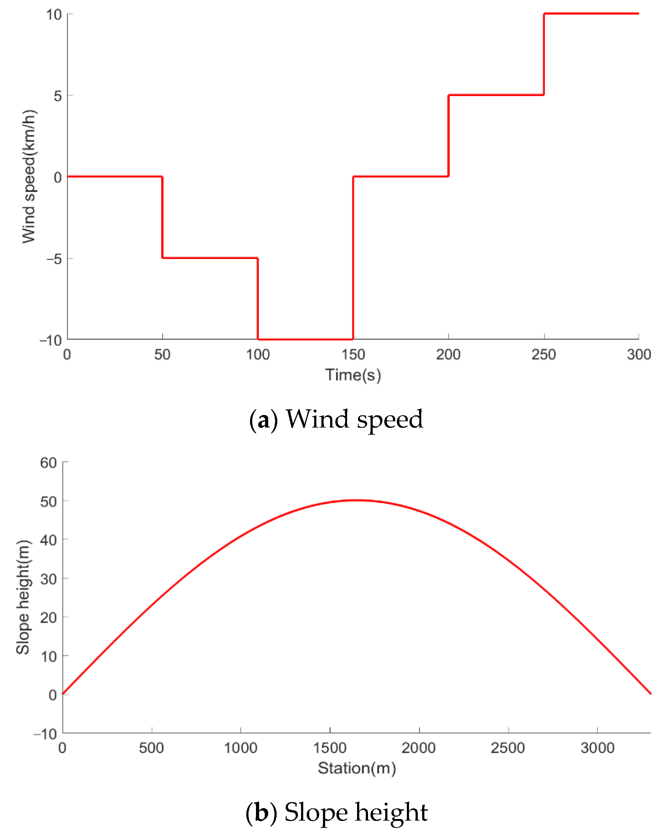
In the case of wind speed change, the wind speed and vehicle speed curves are set as shown in Figure 7, where wind speed greater than zero means downwind driving, and wind speed less than zero means headwind driving.

Figure 7.
Wind speed and vehicle speed curves.
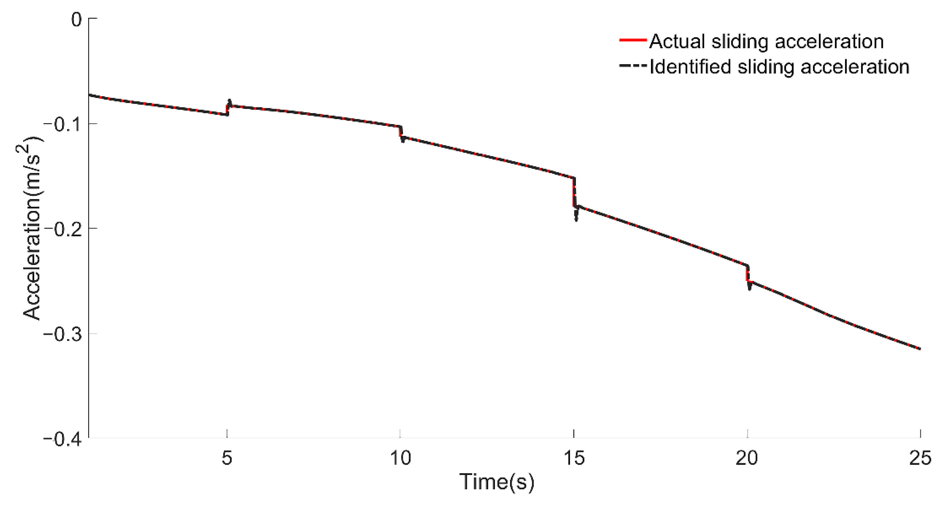
The identification results of sliding acceleration under the change of wind speed are shown in Figure 8 and Figure 9. It can be seen that when the wind speed does not change, the absolute value of the sliding acceleration increases with the increase of vehicle speed, and the change curve of the identified sliding acceleration basically matches with the actual sliding acceleration curve. When the wind speed changes suddenly, there is a deviation between the identified value and the actual value, but the identified value can quickly follow the actual value.

Figure 8.
Sliding acceleration under wind speed variation.
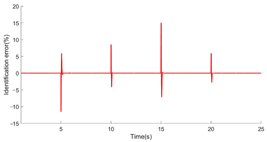
Figure 9.
Identification error under wind speed variation.
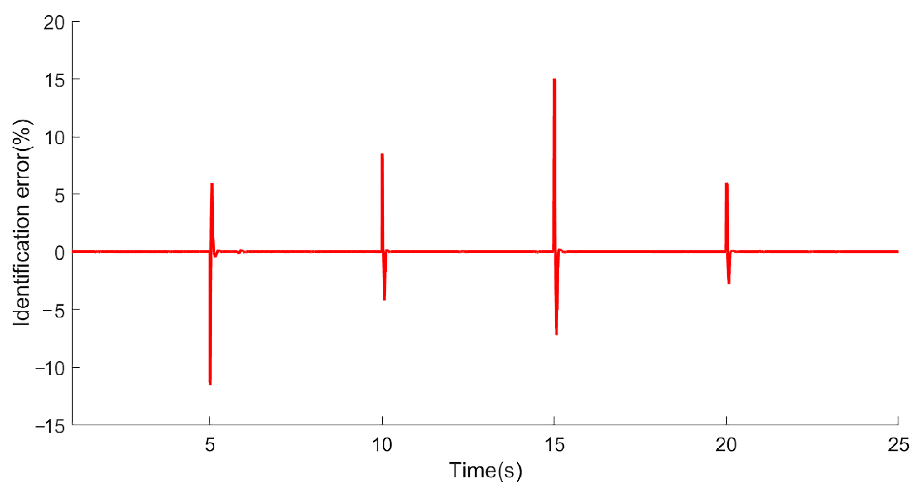
Figure 9 shows the identification error under the change of wind speed. It can be seen that the identification error rate is only high at the sudden change point of wind speed. As the wind speed gradually stabilizes, the identification error rate soon converges to 0. Take a closer look at the identification error rate at the sudden change point of wind speed, it can be seen that the identification error rate has been controlled within 16%. The larger the wind speed sudden change is, the larger the identification error rate is.
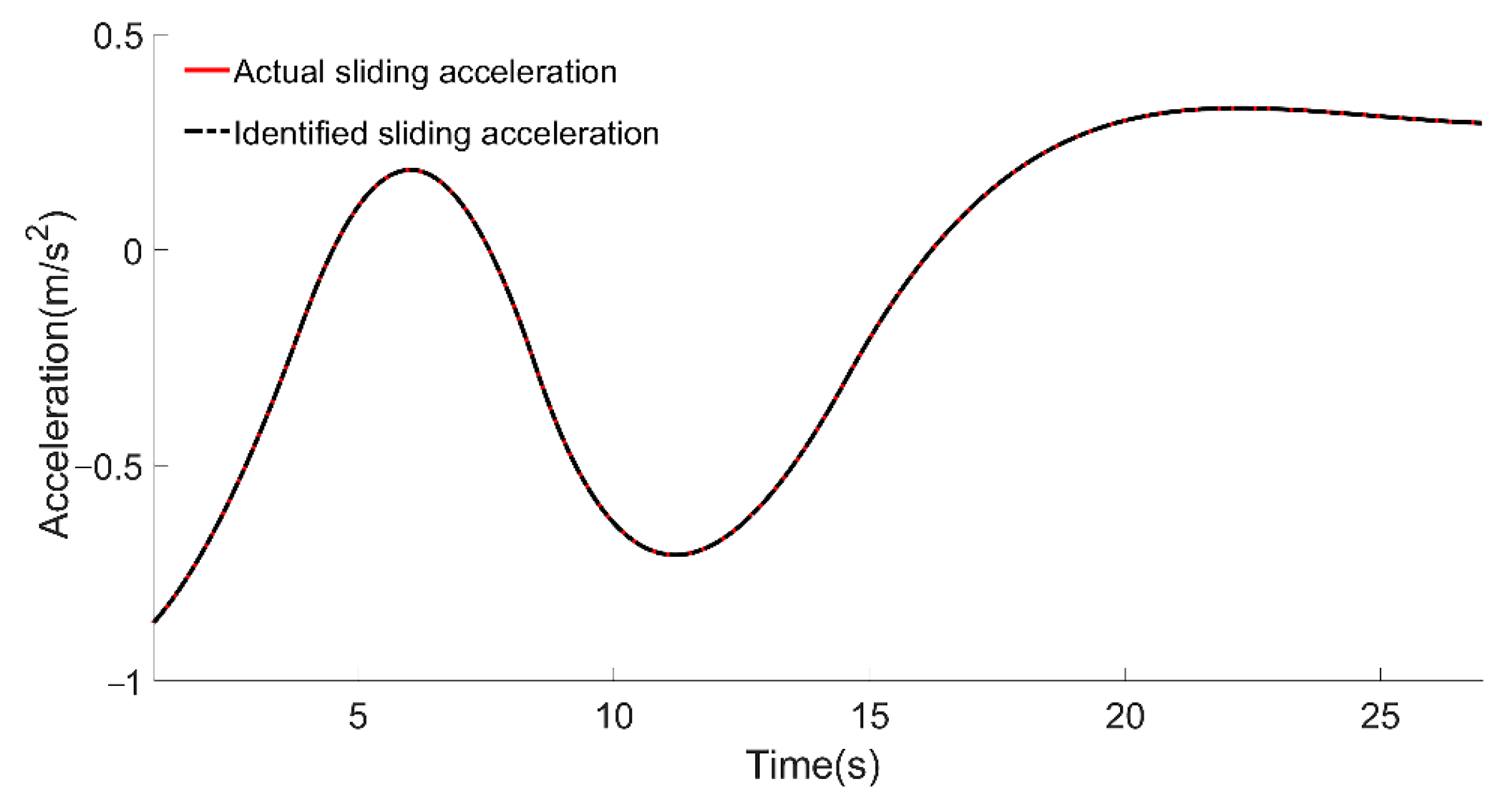
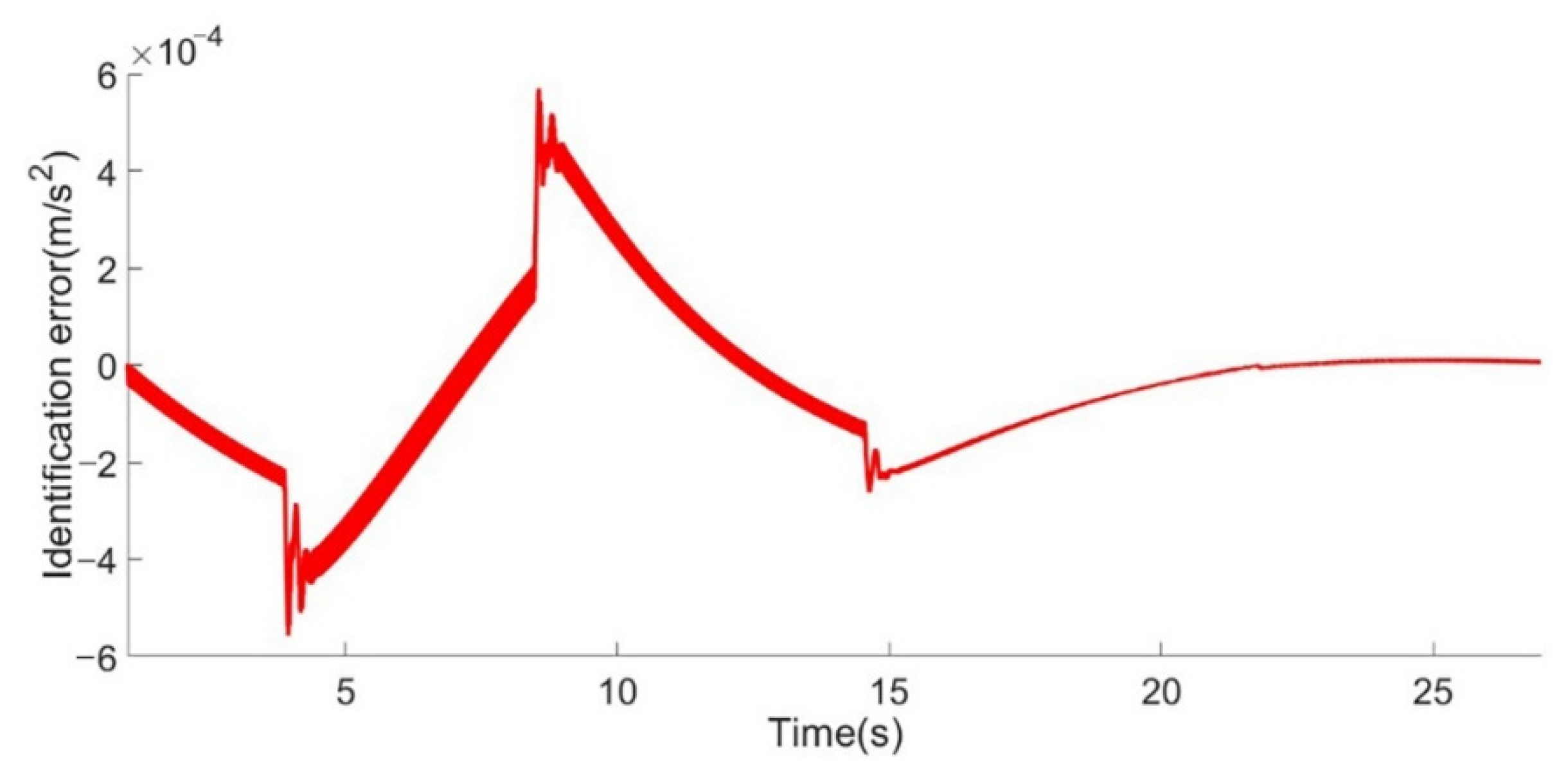
In the case of road slope change, the slope height and vehicle speed curves are shown in Figure 10. The identification results of sliding acceleration under the change of road slope are shown in Figure 11 and Figure 12. It can be seen that when the vehicle is decelerating on the slope, the identified sliding acceleration fits well with the actual sliding acceleration. As the identification error is so small, the difference between the identified value and the actual value is used to express the identification error. Compared with the simulation results under wind speed variation, the identification error under slope height variation is much smaller because the road slope change is much slower than the wind speed change.
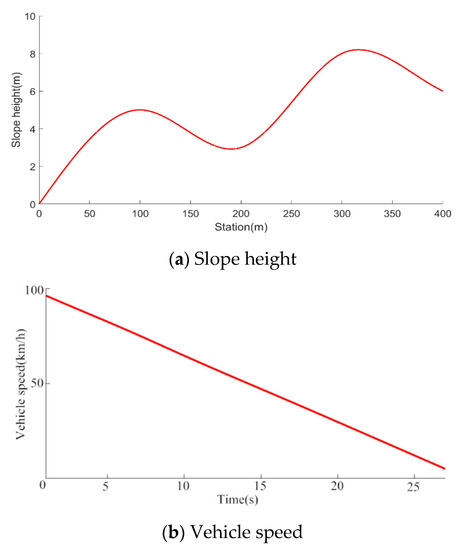
Figure 10.
Slope height and vehicle speed curve.
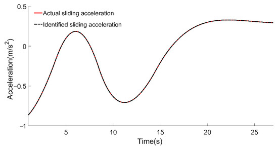
Figure 11.
Sliding acceleration under slope height variation.
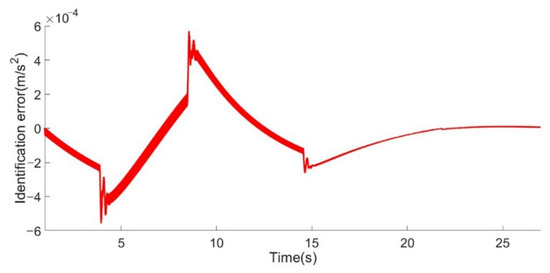
Figure 12.
Identification error under slope height variation.
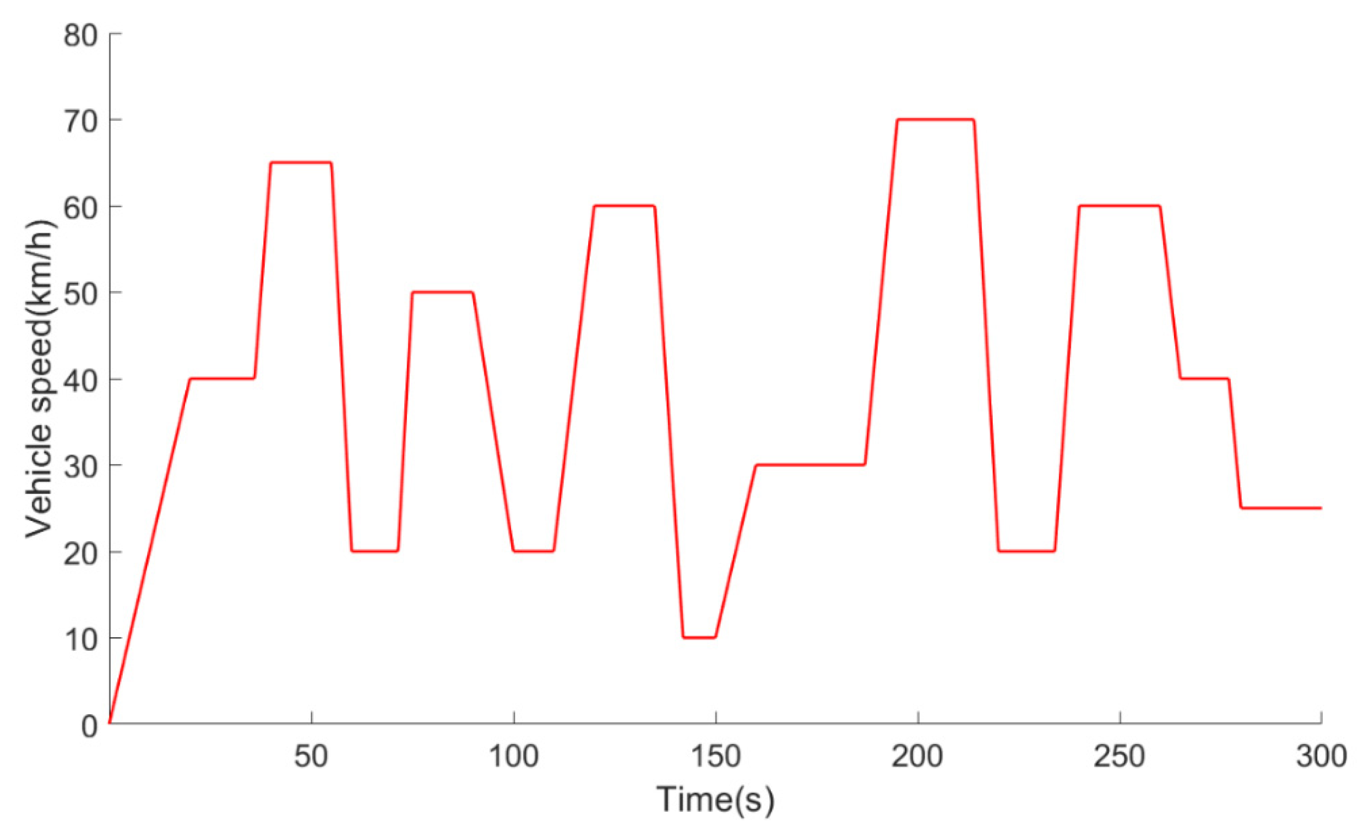
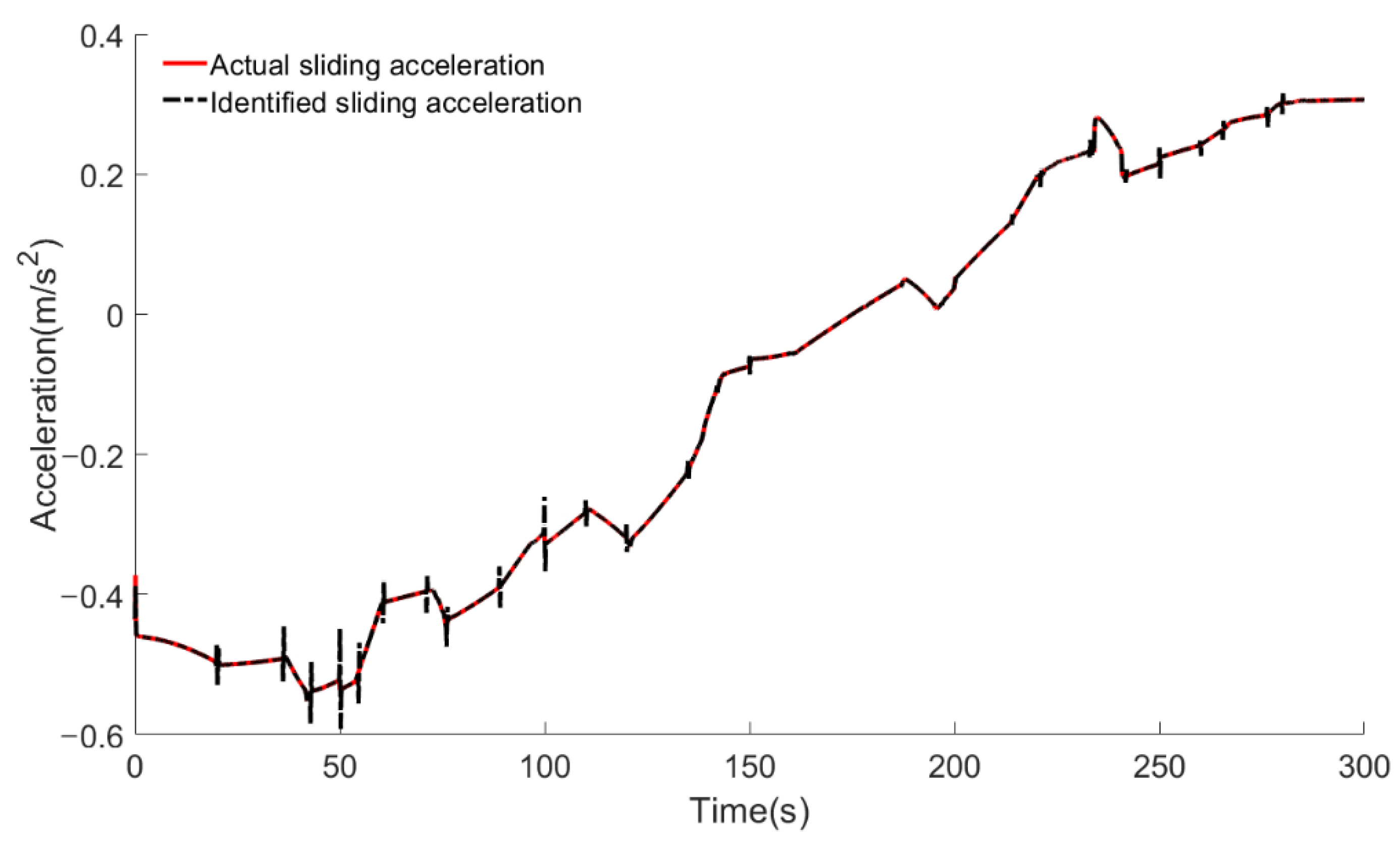
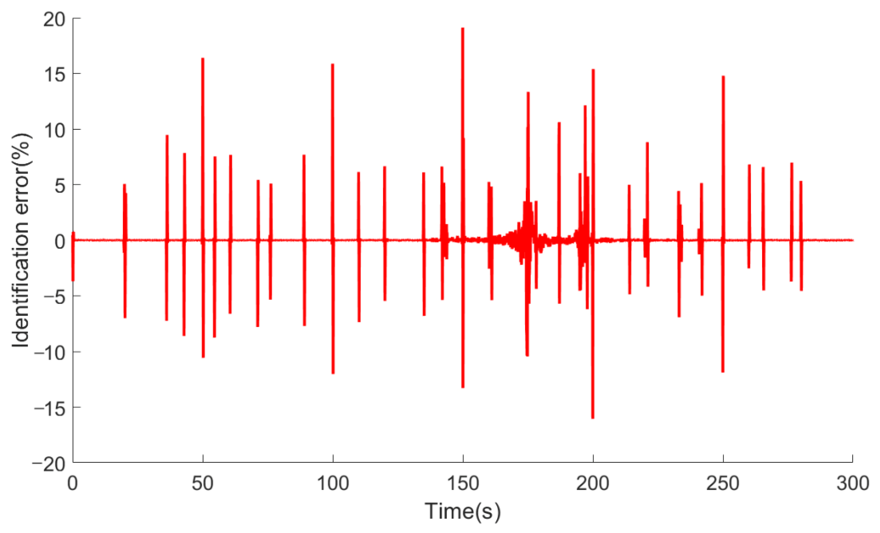
In the actual driving process, wind speed and road slope interference usually occur simultaneously, and measurement disturbances will also have an impact on the identification results. To verify the robustness of the sliding acceleration identification model under multiple disturbances, the wind speed and road slope are set according to Figure 13, the desired vehicle speed is set according to Figure 14, while Gaussian white noise is added to the input signals to make the measurement error reach 5%. Figure 15 and Figure 16 show the identification results of sliding acceleration. It can be seen that the identification error of sliding acceleration increases slightly after considering wind speed, road slope and measurement disturbances, but it can still converge quickly, showing the robustness of the sliding acceleration identification model.

Figure 13.
Wind speed and slope height curves.
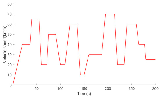
Figure 14.
Desired vehicle speed.
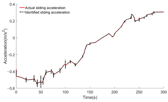
Figure 15.
Sliding acceleration under wind speed and slope height variation.
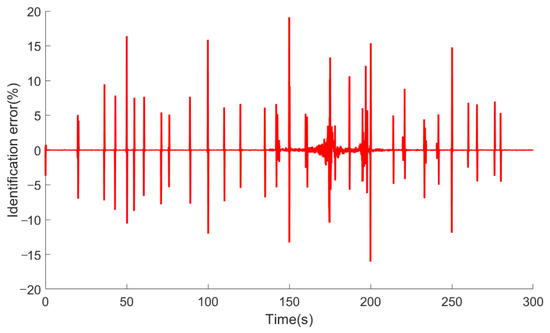
Figure 16.
Identification error under wind speed and slope height variation.
6.2. Simulation and Analysis of the ACC Strategy
To verify the improved performance of the proposed ACC strategy, several comparative simulations under wind speed and road slope change conditions are carried out. The conventional MPC-based ACC strategy is selected as the comparison object, which has two parts less than the proposed ACC strategy, namely, the sliding acceleration identification model and the mode switching optimization. Because the compared ACC strategy cannot obtain the sliding acceleration in real-time, its mode switching boundary is set to 0. Figure 17, Figure 18, Figure 19, Figure 20, Figure 21, Figure 22, Figure 23, Figure 24 and Figure 25 show the simulation results of the two ACC strategies, where the wind speed and road slope are set according to Figure 13, the initial inter-vehicle distance is set to 20 m, and the speed of the lead vehicle is set according to Figure 14.
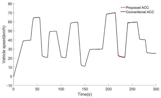
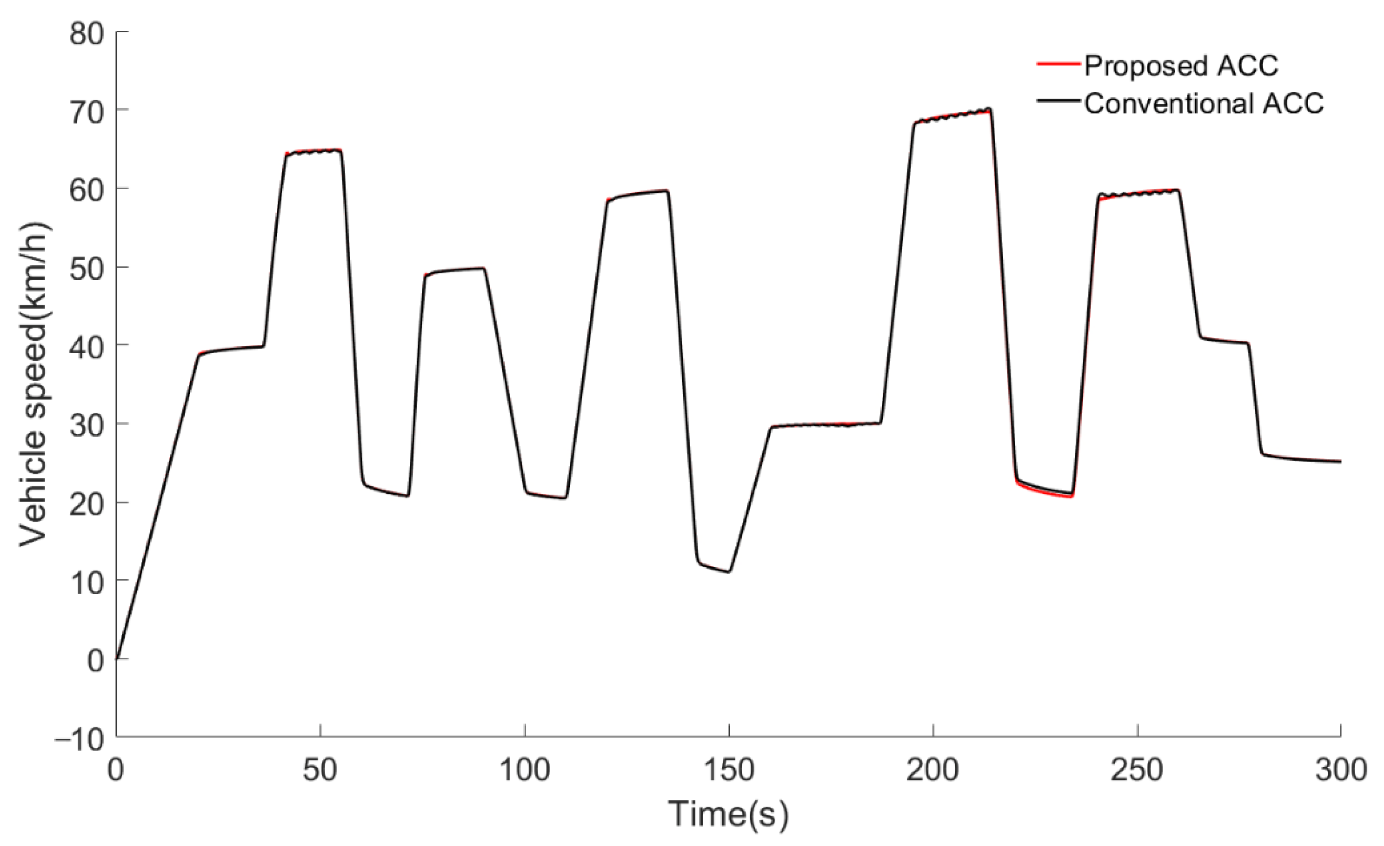
Figure 17.
Vehicle speed.
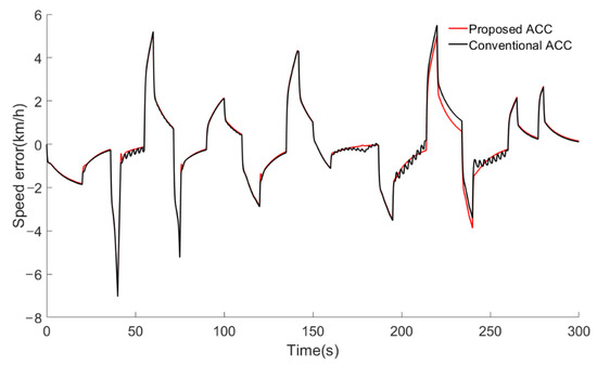
Figure 18.
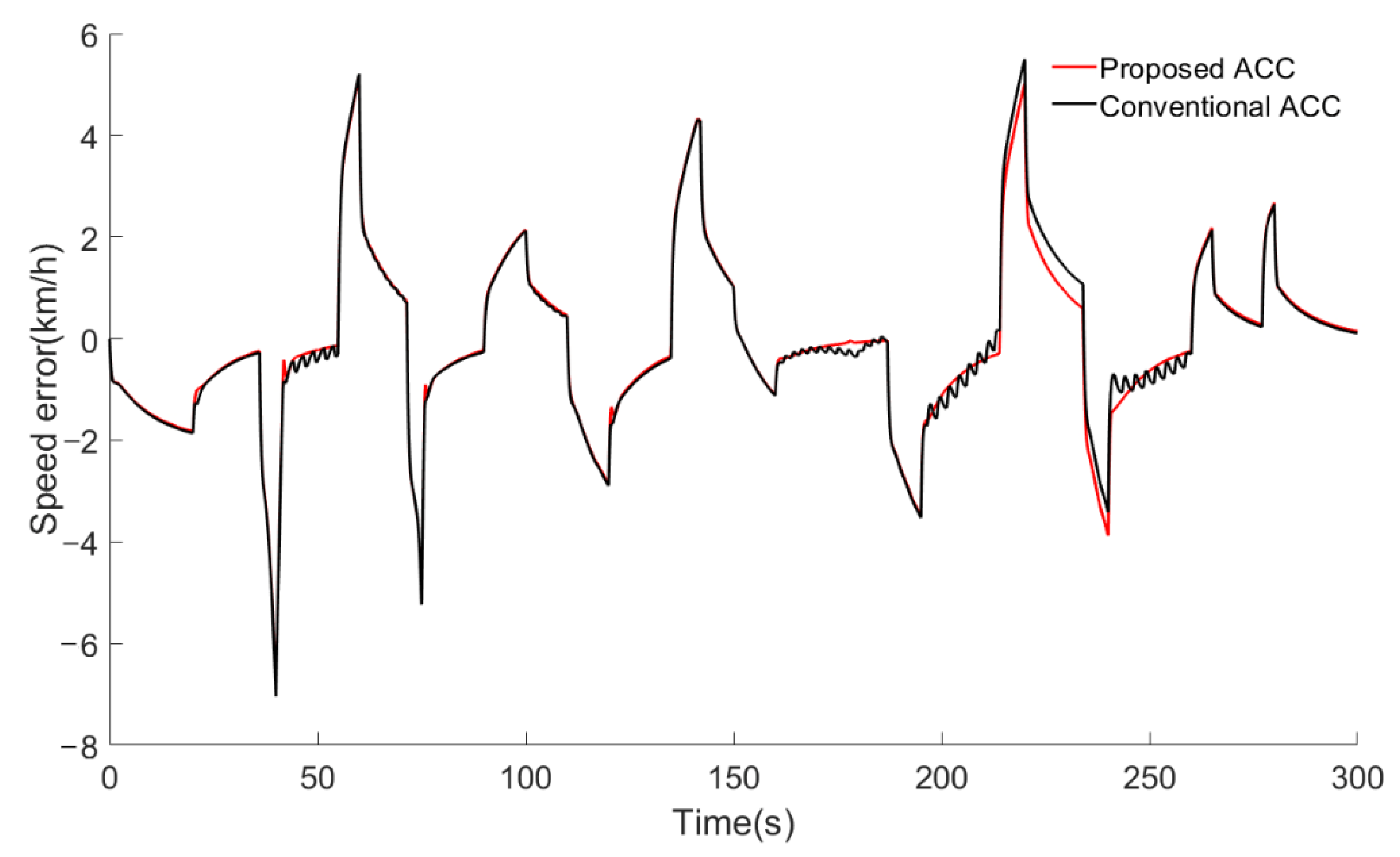
Speed error.
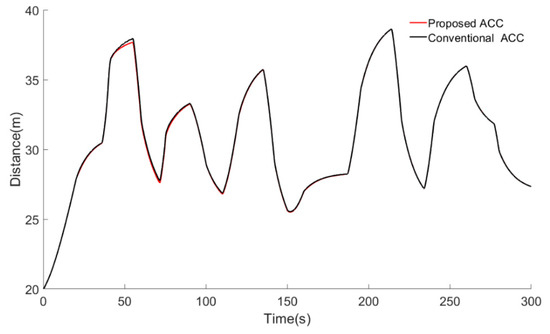
Figure 19.
Inter-vehicle distance.
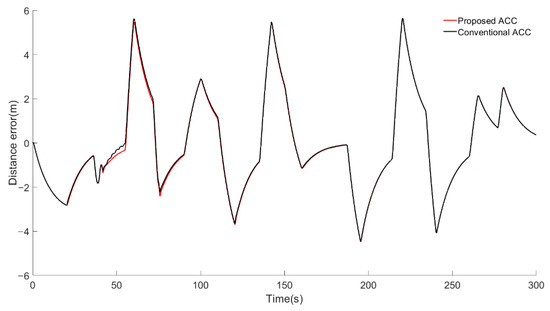
Figure 20.
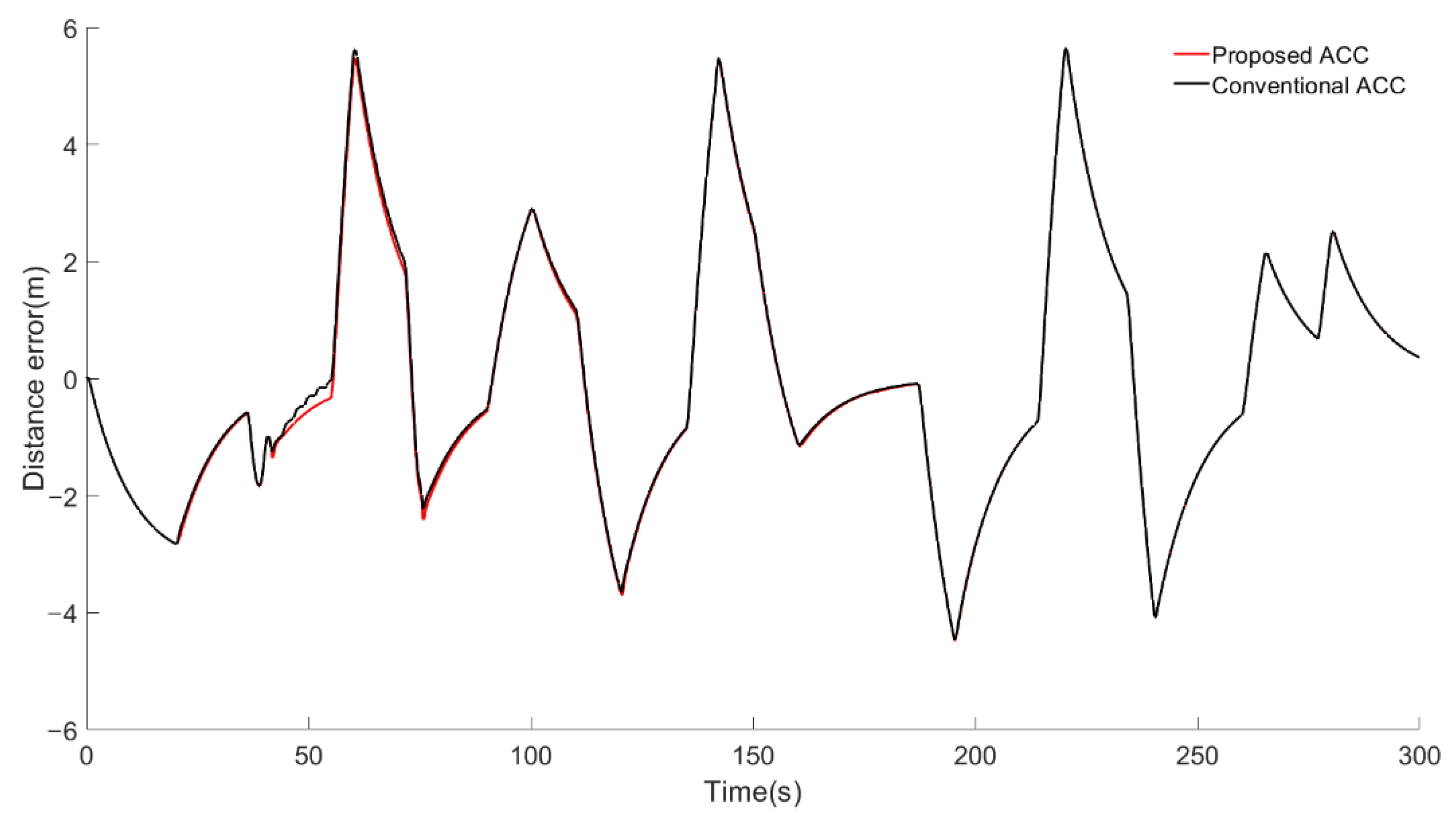
Distance error.
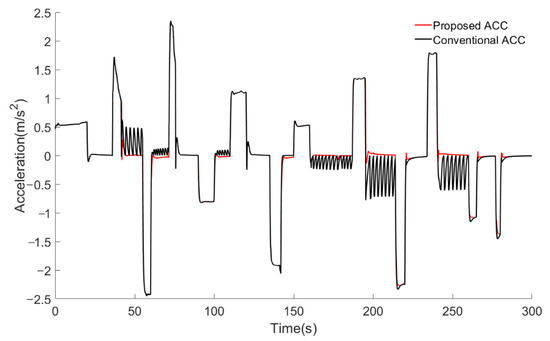
Figure 21.
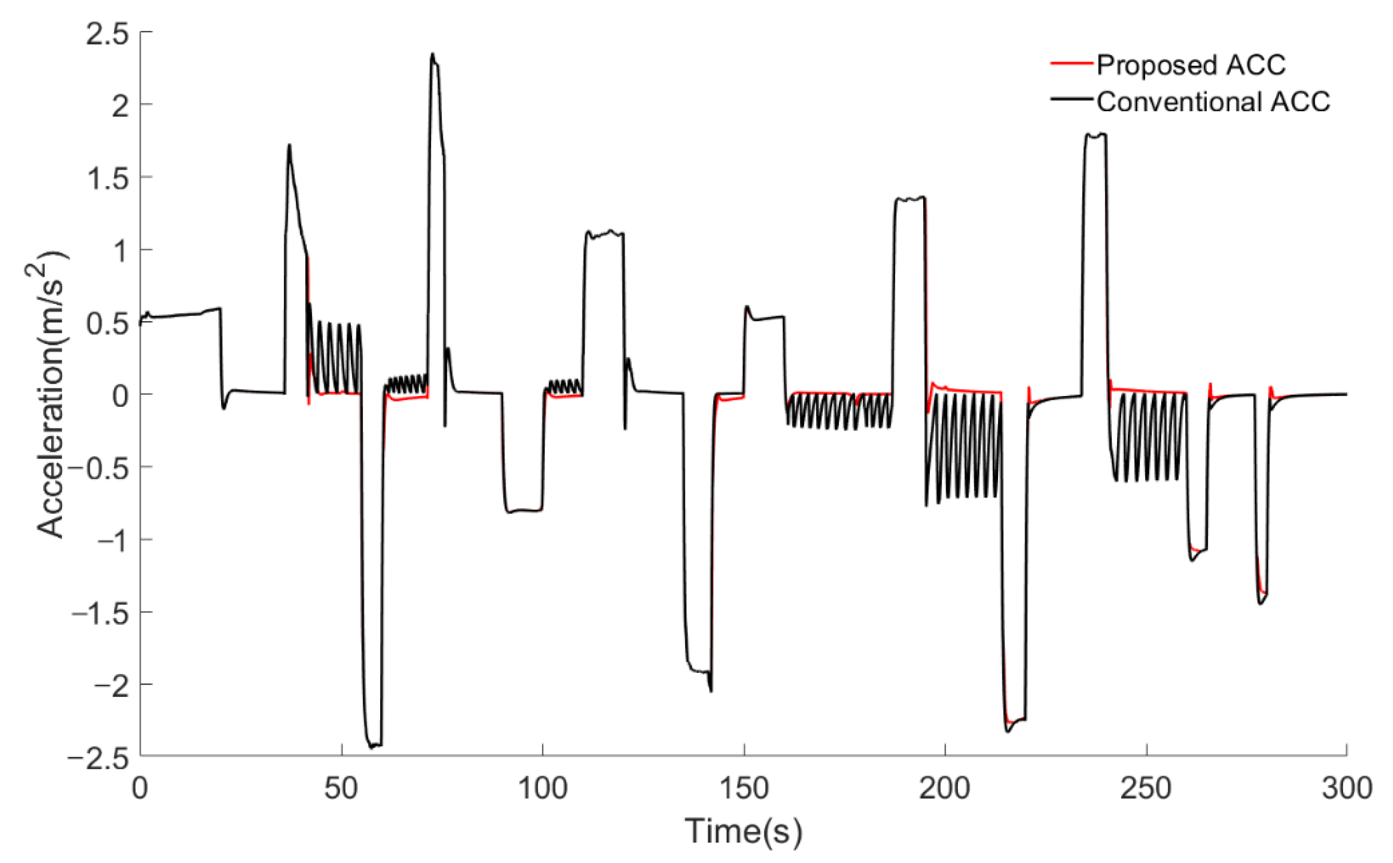
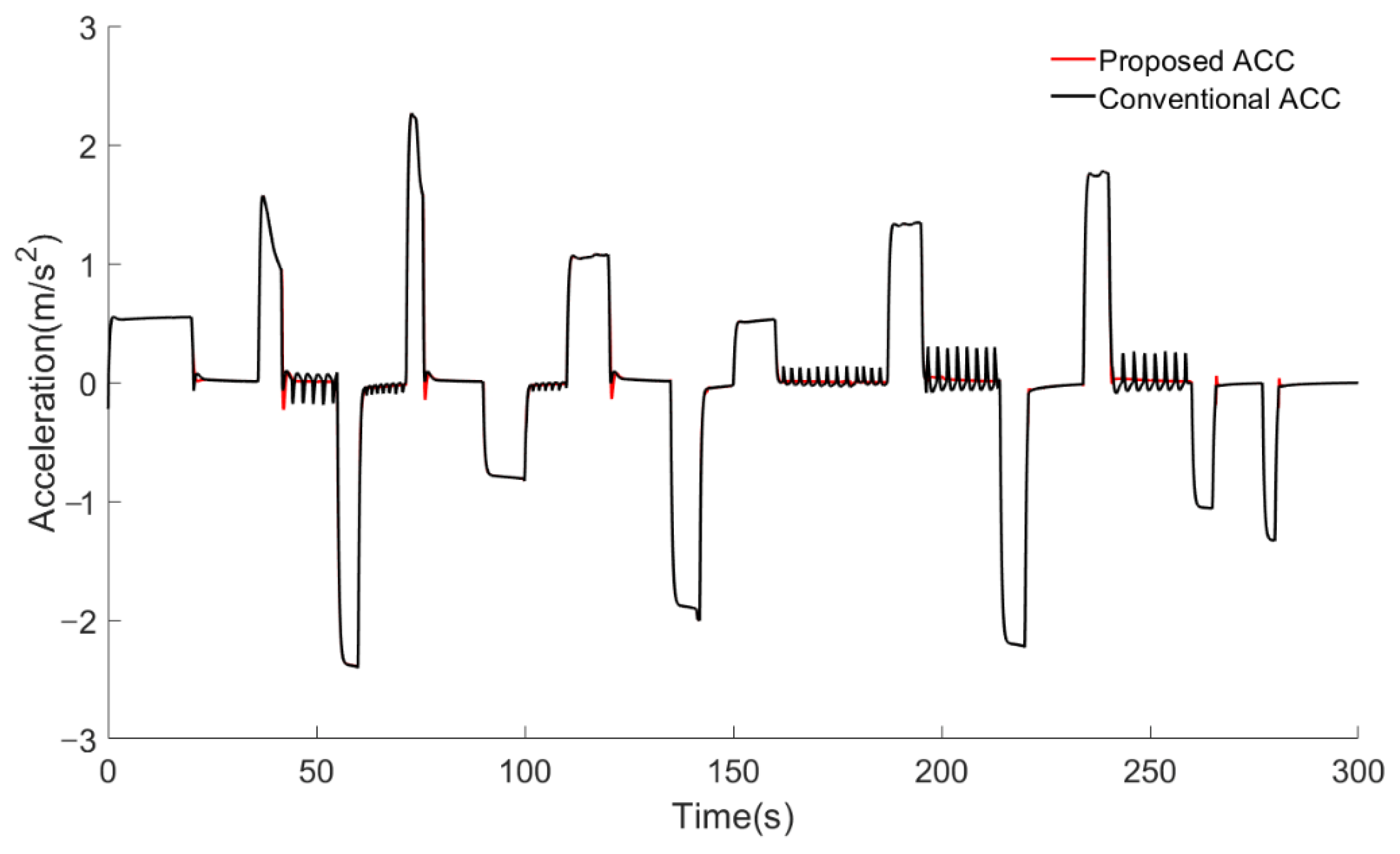
Desired vehicle acceleration.
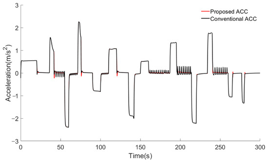
Figure 22.
Actual vehicle acceleration.
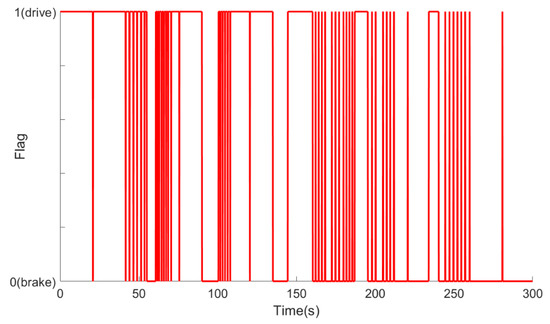
Figure 23.
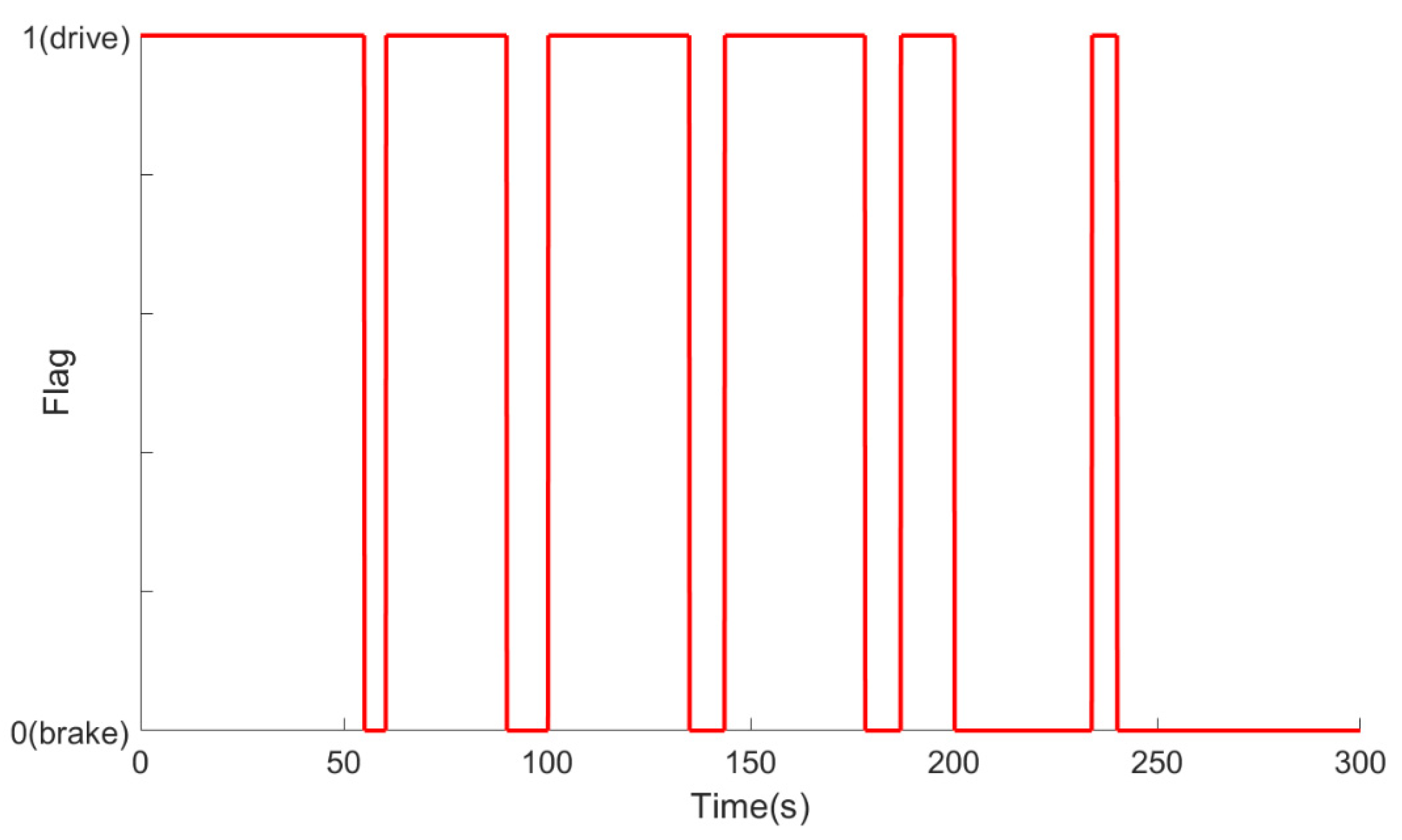
Flag status of conventional ACC.
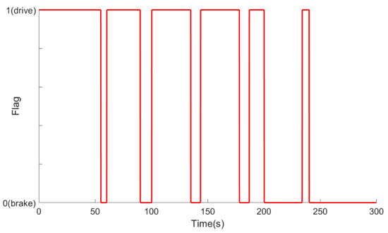
Figure 24.
Flag status of proposed ACC.
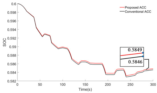
Figure 25.
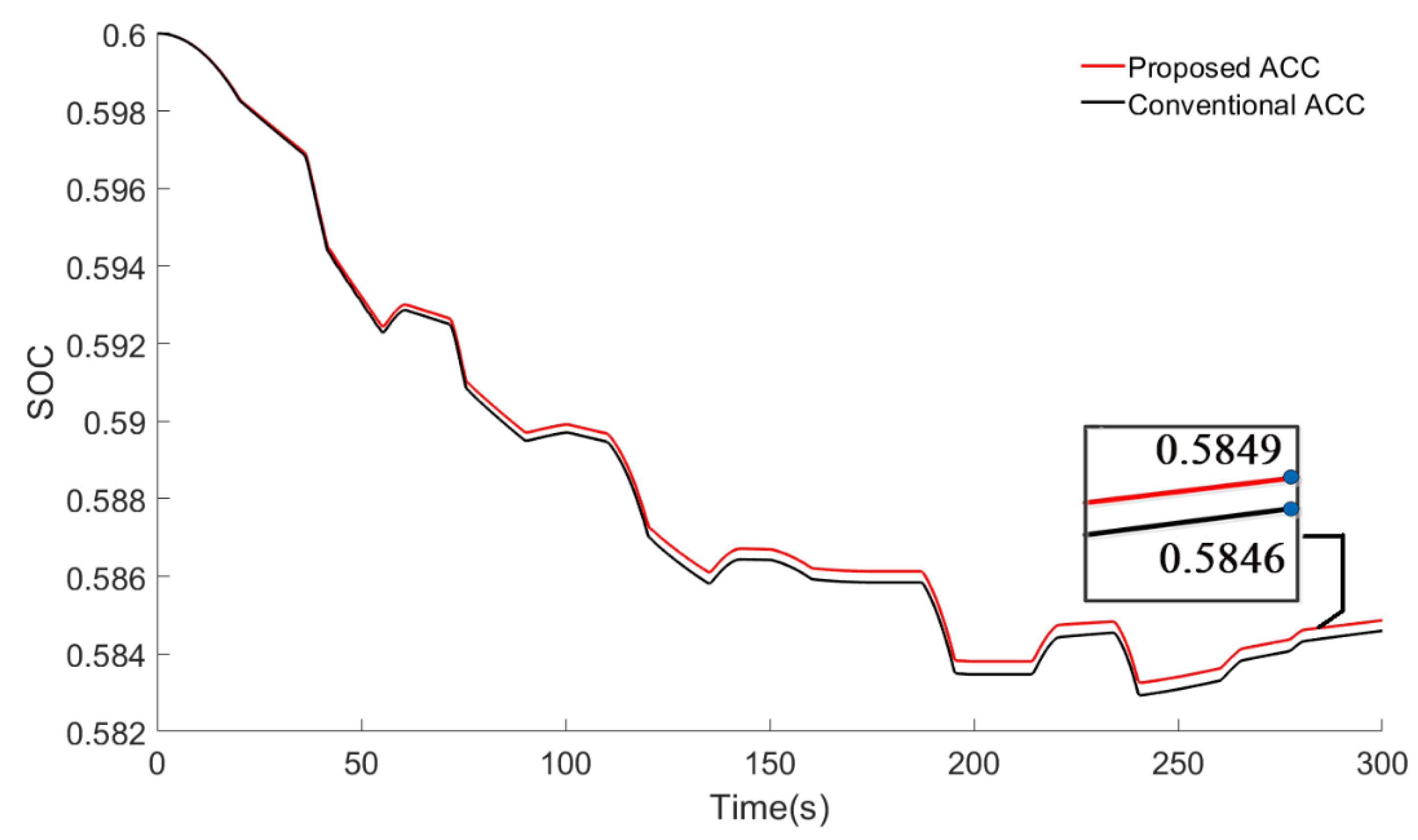
State of charge (SOC).
The speed and distance curves of the two ACC strategies are shown in Figure 17 and Figure 19, and it can be seen that the two control strategies have similar performance in speed following and distance following. When it comes to the speed error and distance error of the two ACC strategies, Figure 18 and Figure 20 show that both ACC strategies can maintain the speed error within 10 km/h and the distance error within 6 m, which can meet driving needs. Furthermore, the speed error and distance error curves of the two ACC strategies approximately overlap when the lead vehicle accelerates or decelerates. But when the lead vehicle drives at a constant speed, the speed error and distance error curves of the two ACC strategies will deviate. The reason is that the objective functions of the two strategies differ only in the mode switching optimization. As the host vehicle seldom switches between driving and braking when the lead vehicle accelerates or decelerates, the mode switching frequency remains 0 in most cases, which means that the mode switching optimization hardly plays a role in the calculation of the desired acceleration. Therefore, the speed error and distance error curves of the two ACC strategies approximately overlap at this time. However, when the lead vehicle drives at a constant speed, the host vehicle will often switch between driving and braking to keep a reasonable distance from the lead vehicle. At this time, the mode switching optimization will influence the calculation of the desired acceleration, leading to the deviation of the speed error and distance error curves of the two strategies.
To further compare the comfort performance of the two ACC strategies, the acceleration curves for both strategies are given in Figure 21 and Figure 22. It can be seen that when the conventional ACC strategy works near the fixed switching boundary, the vehicle acceleration fluctuates greatly. According to the flag status in Figure 23 (1 represents the driving mode, 0 represents the braking mode), the conventional ACC strategy switches frequently between the driving mode and the braking mode. That is because the actual sliding acceleration is always changing with wind speed, road slope and vehicle speed. To adapt to sliding acceleration changes, the vehicle should adjust its working modes all the time. For example, at the 50th second of the simulation, the actual sliding acceleration is less than zero under the influence of road slope and wind speed. To keep the vehicle moving at a constant speed, the vehicle must be in the driving mode. However, the conventional ACC strategy cannot adjust the mode switching logic according to the change of the external environment. As a result, the vehicle may enter the braking mode by mistake. Once the mode is judged wrong, the tracking error will increase. To reduce the error, the conventional ACC strategy will frequently switch between driving and braking mode for feedback correction, which will lead to the fluctuation of acceleration. Furthermore, from Figure 17, Figure 18, Figure 19 and Figure 20, it can be seen that the frequent switching of driving and braking will not only cause fluctuations in acceleration but also in its speed and inter-vehicle distance, resulting in poor comfort.
In contrast, since the proposed ACC strategy can identify the sliding acceleration online and introduce the sliding acceleration into the MPC controller, the problem of frequent mode switching under the changing environment has been effectively solved. From the results shown in Figure 24, we can see that when the desired acceleration is next to zero, the vehicle is always in the correct working mode, and the mode switching frequency of the proposed ACC strategy is significantly reduced, which not only improves the comfort performance but also avoids component wear and extends the operating life of the vehicle. As for the comfort performance of the proposed ACC strategy, it can be seen from Figure 17, Figure 18, Figure 19, Figure 20, Figure 21 and Figure 22 that no matter how the road slope and wind speed change, the vehicle is always kept in a stable running state. Compared to the conventional ACC strategy, the fluctuations of the vehicle speed, inter-vehicle distance, desired acceleration, and actual acceleration of the proposed ACC strategy are greatly reduced when the vehicle is driving at a constant speed.
Benefit from the mode switching optimization, the proposed ACC strategy also has an improvement in terms of vehicle economy. Figure 25 shows the State of charge (SOC) curves of the two ACC strategies; it can be seen that due to the inclusion of the braking force distribution strategy, the battery SOC will increase when the vehicle is braking with high intensity, which means that both strategies can effectively recover the braking energy. When it comes to the economy of the two strategies, Table 2 shows that the average energy consumption of the conventional ACC strategy is 4.87 kWh/100 km, and in contrast, the average energy consumption of the proposed ACC strategy is 4.77 kWh/100 km, which means that an improvement of 2.05% in power is achieved in this driving scenario.
Table 2.
Energy consumption results.
Since the proposed strategy adds the sliding acceleration identification model and mode switching optimization moreso than the conventional strategy, it needs higher computational efficiency. In the aforementioned simulation process, the actual running time of the conventional strategy is 239 s. In contrast, the proposed strategy needs 272 s to complete the simulation. As the actual running time required by both strategies is less than 300 s, both strategies have the potential to be applied in a real-time environment.
7. Conclusions
In this paper, a novel ACC strategy for electric vehicles was proposed, which mainly consisted of a sliding acceleration identification model and an MPC controller. The sliding acceleration identification model was designed based on the MFF-RLS algorithm. By introducing the identified sliding acceleration into the MPC controller, the economy, comfort and following performance of the vehicle could be optimized. The simulation results show that the proposed strategy can accurately identify the sliding acceleration under the interference of wind speed change and slope height change. Compared with the conventional MPC-based ACC strategy, the strategy proposed in this paper has similar performance in speed following and distance following under disturbances, but it significantly reduces the switching frequency between driving and braking modes. Benefitting from that, the comfort and economy of the vehicle are significantly improved. In the terms of comfort, the proposed strategy greatly reduces the vehicle acceleration fluctuation and speed fluctuation. With respect to the economy, the energy consumption of the proposed strategy is reduced by 2.05%.
In practice, the estimation results of the sliding acceleration are influenced by the measurement disturbance, and the MPC algorithm requires high running efficiency. To further verify the effectiveness of the proposed strategy, we will apply the proposed ACC strategy to a real vehicle in the future. In addition, we will study the driver’s behavior characteristics to make the ACC system more suitable to the driver’s needs.
Author Contributions
Conceptualization, L.C. and Y.X.; methodology, software, validation, Y.X., D.Z. and C.C.; investigation, resources, writing—original draft preparation, writing—review and editing, visualization; supervision; project administration, L.C., Y.X., D.Z. and C.C. All authors have read and agreed to be published version of the manuscript.
Funding
This research was funded by key research and development plan in Tianjin (20YFZCGX00770).
Institutional Review Board Statement
Not applicable.
Informed Consent Statement
Not applicable.
Conflicts of Interest
The authors declare no conflict of interests.
References
- Chen, S.M.; He, L.Y. Welfare loss of China’s air pollution: How to make personal vehicle transportation policy. China Econ. Rev. 2014, 31, 106–118. [Google Scholar] [CrossRef]
- Gao, J.; Chen, H.; Li, Y.; Chen, J.; Zhang, Y.; Dave, K.; Huang, Y. Fuel consumption and exhaust emissions of diesel vehicles in worldwide harmonized light vehicles test cycles and their sensitivities to eco-driving factors. Energy Convers. Manag. 2019, 196, 605–613. [Google Scholar] [CrossRef]
- Maimaris, A.; Papageorgiou, G. A review of intelligent transportation systems from a communications technology perspective. In Proceedings of the IEEE Conference on Intelligent Transportation Systems, Rio de Janeiro, Brazil, 1–4 November 2016; pp. 54–59. [Google Scholar]
- Zhang, J.; Wang, F.Y.; Wang, K.; Lin, W.H.; Xu, X.; Chen, C. Data-driven intelligent transportation systems: A survey. IEEE Trans. Intell. Transp. Syst. 2011, 12, 1624–1639. [Google Scholar] [CrossRef]
- Wu, X.; He, X.; Yu, G.; Harmandayan, A.; Wang, Y. Energy-Optimal Speed Control for Electric Vehicles on Signalized Arterials. IEEE Trans. Intell. Transp. Syst. 2015, 16, 2786–2796. [Google Scholar] [CrossRef]
- Akhegaonkar, S.; Nouvelière, L.; Glaser, S.; Holzmann, F. Smart and green ACC: Energy and safety optimization strategies for EVs. IEEE Trans. Syst. Man Cybern. 2018, 48, 142–153. [Google Scholar] [CrossRef] [Green Version]
- Kuang, X.; Zhao, F.; Hao, H.; Liu, Z. Intelligent vehicles’ effects on Chinese traffic: A simulation study of cooperative adaptive cruise control and intelligent speed adaption. In Proceedings of the IEEE Conference on Intelligent Transportation Systems, Maui, HI, USA, 4–7 November 2018; pp. 368–373. [Google Scholar]
- Arnaout, G.M.; Arnaout, J.P. Exploring the effects of cooperative adaptive cruise control on highway traffic flow using microscopic traffic simulation. Transp. Plan. Technol. 2014, 37, 186–199. [Google Scholar] [CrossRef]
- Hülsebusch, D.; Salfeld, M.; Xia, Y.; Gauterin, F. Adaptive cruise control: A behavioral assessment of following traffic participants due to energy efficient driving strategies. Lect. Notes Electr. Eng. 2013, 200, 209–220. [Google Scholar] [CrossRef]
- Goñi-Ros, B.; Schakel, W.J.; Papacharalampous, A.E.; Wang, M.; Knoop, V.L.; Sakata, I.; van Arem, B.; Hoogendoorn, S.P. Using advanced adaptive cruise control systems to reduce congestion at sags: An evaluation based on microscopic traffic simulation. Transp. Res. Part C 2019, 102, 411–426. [Google Scholar] [CrossRef]
- Meier, J.N.; Kailas, A.; Adla, R.; Bitar, G.; Moradi-Pari, E.; Abuchaar, O.; Ali, M.; Abubakr, M.; Deering, R.; Ibrahim, U.; et al. Implementation and evaluation of cooperative adaptive cruise control functionalities. IET Intell. Transport. Syst. 2018, 12, 1110–1115. [Google Scholar] [CrossRef]
- Weißmann, A.; Görges, D.; Lin, X. Energy-optimal adaptive cruise control combining model predictive control and dynamic programming. Control. Eng. Pract. 2018, 72, 125–137. [Google Scholar] [CrossRef]
- Abdullah, R.; Hussain, A.; Warwick, K.; Zayed, A. Autonomous intelligent cruise control using a novel multiple-controller framework incorporating fuzzy-logic-based switching and tuning. Neurocomputing 2008, 71, 2727–2741. [Google Scholar] [CrossRef]
- Ganji, B.; Kouzani, A.Z.; Khoo, S.Y.; Shams-Zahraei, M. Adaptive cruise control of a HEV using sliding mode control. Expert Syst. Appl. 2014, 41, 607–615. [Google Scholar] [CrossRef]
- Zhao, D.; Xia, Z.; Zhang, Q. Model-Free Optimal Control Based Intelligent Cruise Control with Hardware-in-the-Loop Demonstration [Research Frontier]. IEEE Comput. Intell. Mag. 2017, 12, 56–69. [Google Scholar] [CrossRef]
- Prabhakar, G.; Selvaperumal, S.; Nedumal Pugazhenthi, P. Fuzzy PD Plus I Control-based Adaptive Cruise Control System in Simulation and Real-time Environment. IETE J. Res. 2019, 65, 69–79. [Google Scholar] [CrossRef]
- Shakouri, P.; Ordys, A. Nonlinear Model Predictive Control approach in design of Adaptive Cruise Control with automated switching to cruise control. Control. Eng. Pract. 2014, 26, 160–177. [Google Scholar] [CrossRef]
- Okuda, H.; Mikami, K.; Tazaki, Y.; Suzuki, T.; Tsuru, N.; Isaji, K. A unified assisting system for longitudinal driving behavior based on model predictive control. In Proceedings of the 2011 IEEE International Conference on Vehicular Electronics and Safety, Beijing, China, 10–12 July 2011; pp. 199–204. [Google Scholar]
- Shuo, Z.; Qiang, Y.; Shihao, L.; Yibo, W.; Xianyong, G. Adaptive cruise hierarchical control strategy based on MPC. Int. J. Veh. Inf. Commun. Syst. 2021, 6, 161–184. [Google Scholar] [CrossRef]
- Bageshwar, V.L.; Garrard, W.L.; Rajamani, R. Model predictive control of transitional maneuvers for adaptive cruise control vehicles. IEEE Trans. Veh. Technol. 2004, 53, 1573–1585. [Google Scholar] [CrossRef]
- Eben Li, S.; Li, K.; Wang, J. Economy-oriented vehicle adaptive cruise control with coordinating multiple objectives function. Veh. Syst. Dyn. 2013, 51, 1–17. [Google Scholar] [CrossRef]
- Kohut, N.; Borrelli, F.; Hedrick, K.; Lamprecht, A.; Lee, J.; Lee, C.H.; Rosario, D. Utilization of intelligent transport systems information to increase fuel economy through engine control. In Proceedings of the 15th World Congress on Intelligent Transport Systems and ITS America Annual Meeting, New York, NY, USA, 16–20 November 2008; pp. 6956–6966. [Google Scholar]
- Yu, K.; Yang, J.; Yamaguchi, D. Model predictive control for hybrid vehicle ecological driving using traffic signal and road slope information. Control Theory Technol. 2015, 13, 17–28. [Google Scholar] [CrossRef]
- Sun, C.; Chu, L.; Guo, J.; Shi, D.; Li, T.; Jiang, Y. Research on adaptive cruise control strategy of pure electric vehicle with braking energy recovery. Adv. Mech. Eng. 2017, 9, 1687814017734994. [Google Scholar] [CrossRef]
- Sakhdari, B.; Azad, N.L. Adaptive Tube-Based Nonlinear MPC for Economic Autonomous Cruise Control of Plug-In Hybrid Electric Vehicles. IEEE Trans. Veh. Technol. 2018, 67, 11390–11401. [Google Scholar] [CrossRef]
- Zhang, J.; Li, Q.; Chen, D. Integrated adaptive cruise control withweight coefficient self-tuning strategy. Appl. Sci. 2018, 8, 978. [Google Scholar] [CrossRef] [Green Version]
- Nie, Z.; Farzaneh, H. Adaptive cruise control for eco-driving based on model predictive control algorithm. Appl. Sci. 2020, 10, 5271. [Google Scholar] [CrossRef]
- Li, S.E.; Guo, Q.; Xu, S.; Duan, J.; Lii, S.; Li, C.; Su, K. Performance Enhanced Predictive Control for Adaptive Cruise Control System Considering Road Elevation Information. IEEE Trans. Intell. Veh. 2017, 2, 150–160. [Google Scholar] [CrossRef]
- Ma, H.; Chu, L.; Guo, J.; Wang, J.; Guo, C. Cooperative Adaptive Cruise Control Strategy Optimization for Electric Vehicles Based on SA-PSO with Model Predictive Control. IEEE Access 2020, 8, 225745–225756. [Google Scholar] [CrossRef]
- Deng, W.; Bian, N.; Jiang, Y.; He, R.; Yang, S.; Wang, S. Hierarchical Framework for Adaptive Cruise Control with Model Predictive Control Method; SAE International: Warrendale, PA, USA, 2017. [Google Scholar]
- Li, S.E.; Gao, F.; Cao, D.; Li, K. Multiple-Model Switching Control of Vehicle Longitudinal Dynamics for Platoon-Level Automation. IEEE Trans. Veh. Technol. 2016, 65, 4480–4492. [Google Scholar] [CrossRef]
- Zhang, R.; Zhao, Y.; Chen, S.; Wu, Z.; Yang, L. Longitudinal dynamic control under complex driving conditions via fuzzy logic sliding-mode control. In Proceedings of the 2019 IEEE International Conference on Mechatronics and Automation, Tianjin, China, 4–8 August 2019; pp. 1161–1166. [Google Scholar]
- Lihua, L.; Jihong, C.; Fangwei, Z. Integrated Adaptive Cruise Control design considering the optimization of switching between throttle and brake. In Proceedings of the IEEE Intelligent Vehicles Symposium, Gothenburg, Sweden, 19–22 June 2016; pp. 1162–1167. [Google Scholar]
- Zhao, D.; Chu, L.; Xu, N.; Sun, C.; Xu, Y. Development of a cooperative braking system for front-wheel drive electric vehicles. Energies 2018, 11, 378. [Google Scholar] [CrossRef] [Green Version]
- Li, S.B.; Li, K.Q.; Rajamani, R.; Wang, J.Q. Model Predictive Multi-Objective Vehicular Adaptive Cruise Control. IEEE Trans. Control. Syst. Technol. 2011, 19, 556–566. [Google Scholar] [CrossRef]
- Moon, S.; Moon, I.; Yi, K. Design, tuning, and evaluation of a full-range adaptive cruise control system with collision avoidance. Control. Eng. Pract. 2009, 17, 442–455. [Google Scholar] [CrossRef]
- Tsai, C.C.; Hsieh, S.M.; Chen, C.T. Fuzzy longitudinal controller design and experimentation for adaptive cruise control and stop&Go. J. Intell. Robot. Syst. 2010, 59, 167–189. [Google Scholar] [CrossRef]
- Kim, H.; Yi, K. Design of a Model Reference Cruise Control Algorithm. SAE Int. J. Passeng. Cars 2012, 5, 440–449. [Google Scholar] [CrossRef]
- Li, Y.; Zheng, L.; Qiao, Y. Fuzzy-PID control method on vehicle longitudinal dynamics system. Zhongguo Jixie Gongcheng/China Mech. Eng. 2006, 17, 99–103. [Google Scholar]
- Gu, Y.; Ding, R. A least squares identification algorithm for a state space model with multi-state delays. Appl. Math. Lett. 2013, 26, 748–753. [Google Scholar] [CrossRef]
- Park, J. Simultaneous estimation based on empirical likelihood and general maximum likelihood estimation. Comput. Stat. Data Anal. 2018, 117, 19–31. [Google Scholar] [CrossRef]
- Lu, J.; Chen, Z.; Yang, Y.; Lv, M. Online Estimation of State of Power for Lithium-Ion Batteries in Electric Vehicles Using Genetic Algorithm. IEEE Access 2018, 6, 20868–20880. [Google Scholar] [CrossRef]
- Wang, F.; Zhang, H.; Li, K.; Lin, Z.; Yang, J.; Shen, X.L. A hybrid particle swarm optimization algorithm using adaptive learning strategy. Inf. Sci. 2018, 436–437, 162–177. [Google Scholar] [CrossRef]
- Sitarz, P.; Powałka, B. Modal parameters estimation using ant colony optimisation algorithm. Mech. Syst. Signal. Process. 2016, 76–77, 531–554. [Google Scholar] [CrossRef]
- Ding, F.; Wang, Y.; Ding, J. Recursive least squares parameter identification algorithms for systems with colored noise using the filtering technique and the auxilary model. Digit. Signal. Process. 2015, 37, 100–108. [Google Scholar] [CrossRef]
- Lao, Z.; Xia, B.; Wang, W.; Sun, W.; Lai, Y.; Wang, M. A novel method for lithium-ion battery online parameter identification based on variable forgetting factor recursive least squares. Energies 2018, 11, 1358. [Google Scholar] [CrossRef] [Green Version]
- Martinez, J.J.; Canudas-de-Wit, C. A safe longitudinal control for adaptive cruise control and stop-and-go scenarios. IEEE Trans. Control Syst. Technol. 2007, 15, 246–258. [Google Scholar] [CrossRef]
- Wächter, A.; Biegler, L.T. On the implementation of an interior-point filter line-search algorithm for large-scale nonlinear programming. Math. Program. 2006, 106, 25–57. [Google Scholar] [CrossRef]
- Janssens, P.; Pipeleers, G.; Swevers, J. A data-driven constrained norm-optimal iterative learning control framework for LTI systems. IEEE Trans. Control Syst. Technol. 2013, 21, 546–551. [Google Scholar] [CrossRef] [Green Version]


Publisher’s Note: MDPI stays neutral with regard to jurisdictional claims in published maps and institutional affiliations. |
© 2021 by the authors. Licensee MDPI, Basel, Switzerland. This article is an open access article distributed under the terms and conditions of the Creative Commons Attribution (CC BY) license (https://creativecommons.org/licenses/by/4.0/).