A Hybrid RRT–PPO Framework for Leg-Based Object Manipulation of Quadruped Robots

Abstract

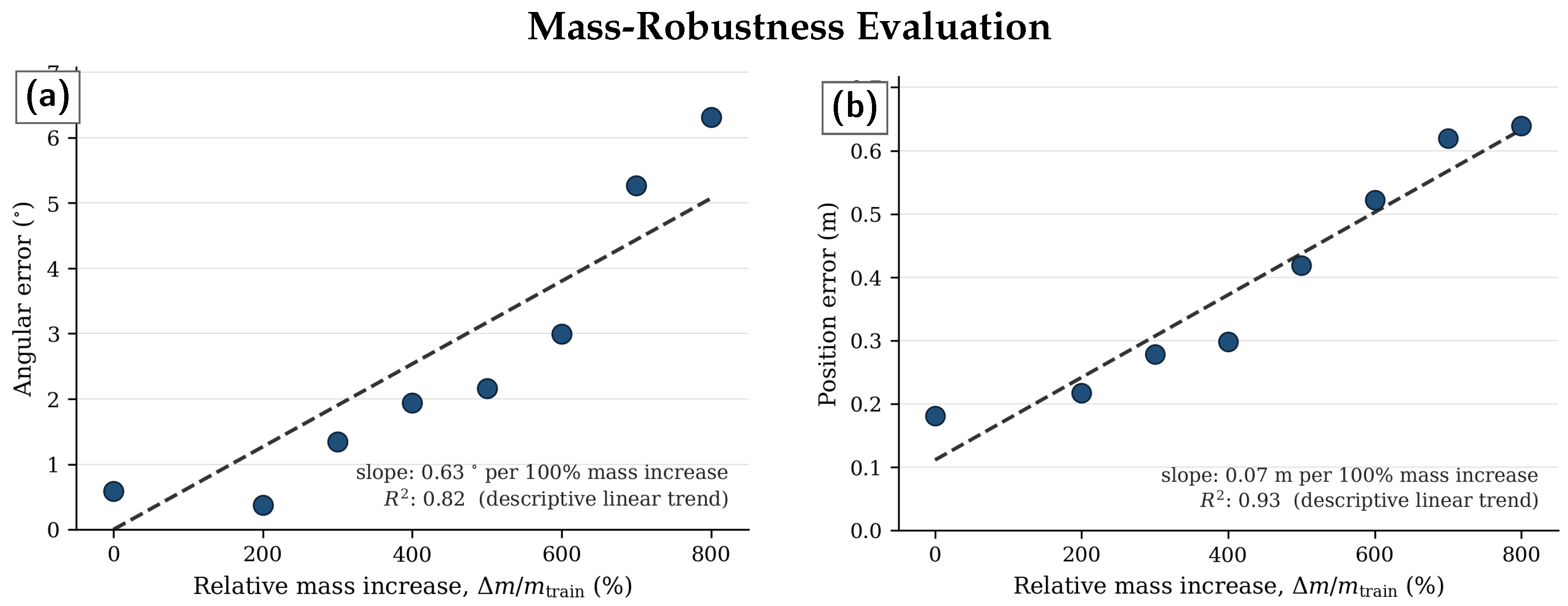
Quadruped robots can extend their utility beyond locomotion by using a leg as a non-prehensile end-effector to push objects, but this requires combining global planning with adaptive contact control. We present a hybrid framework that couples Rapidly exploring Random Trees (RRT) for global motion planning with Proximal Policy Optimization (PPO) for local leg-pushing control, evaluated in a CoppeliaSim simulation of a Spot-like quadruped pushing a box to a goal pose. The PPO action consists of Bézier control-point parameters and a leg-selection index, and the reward combines positional error, angular error, and a stability penalty. The agent learns straight-line pushing. Without retraining, a fixed asymmetric Bézier action induces a consistent rotation at $\omega \approx 4–5\times {10}^{-4}$ rad/s, and the resulting circular arcs are composed—in the spirit of Dubins paths—to follow curved trajectories. For box masses from $0.1$ kg to $0.9$ kg (up to eight times the training mass), angular and position errors grew approximately linearly from $0.59°$ to $6.32°$ and $0.18$ m to $0.64$ m, respectively, with no abrupt divergence. A single learned pushing primitive, combined with sampling-based planning and a deterministic composition rule, generates both straight-line and curved manipulation.

1. Introduction

Quadruped robots have emerged as versatile platforms for operating in unstructured and hazardous environments [1]. Their multi-degree-of-freedom leg mechanisms provide locomotion flexibility over complex, rough terrain that wheeled platforms cannot easily traverse [2,3]. Consequently, central to their effective deployment are locomotion control algorithms, including approaches that combine gait or trajectory generators and model-based components with learning-based policies for stable, robust locomotion [4,5].

Beyond locomotion, enabling legged robots to interact with and manipulate objects in their environment represents a significant frontier in autonomous robotics. While robotic arms are traditionally used for manipulation tasks, quadruped robots can leverage their legs as end-effectors to push, pull, or relocate objects—a capability that extends their utility without requiring additional hardware. However, achieving reliable leg-based manipulation requires the integration of sophisticated motion planning with adaptive control strategies capable of handling the inherent uncertainties of physical interaction.

Motion planning algorithms, such as the Rapidly exploring Random Tree (RRT) [6], have proven effective for navigating complex configuration spaces. RRT and its variants incrementally construct search trees through random sampling, efficiently finding feasible paths in high-dimensional spaces [7,8]. However, classical motion planning alone is insufficient to address the dynamic and contact-rich nature of object manipulation tasks, where the robot must continuously adapt its actions based on environmental feedback.

Reinforcement learning (RL) offers a complementary paradigm, enabling agents to learn effective control policies through trial-and-error interaction with their environment [9,10]. Proximal Policy Optimization (PPO) [11] has emerged as a particularly effective RL algorithm for continuous control tasks, offering stable policy updates through its clipped surrogate objective function. PPO has been successfully applied to robotic manipulation problems such as dexterous in-hand manipulation [12].

This paper presents a hybrid framework that combines RRT-based motion planning with PPO-based reinforcement learning for autonomous leg-based object manipulation by a quadruped robot. The key contributions of this work are:

• A hybrid architecture integrating RRT for global path planning and PPO for local manipulation control, leveraging the strengths of model-based and learning-based approaches.
• A Bézier curve-parameterized leg trajectory representation that enables the RL agent to generate smooth, controllable pushing motions through a compact action space.
• A reward function design incorporating position error, angular error, and stability penalties that effectively guides the learning of box-pushing behaviors.
• A comprehensive robustness analysis demonstrating that the trained agent continues to push objects with masses up to eight times the training mass, with other physical parameters (shape, friction, and surface conditions) held constant.
• An extension of the learned straight-line pushing to curved paths: applying a fixed, asymmetric Bézier pushing action induces a consistent box rotation at a measurable mean rotational speed, and the resulting approximately circular arcs are composed to follow curved trajectories. Dubins path theory [13] provides the conceptual basis for composing straight segments and circular arcs.

The remainder of this paper is organized as follows. Section 2 reviews related work in motion planning and RL for robotic manipulation. Section 3 presents the proposed methodology, including the robot model, RRT-based planning, and RL-based manipulation. Section 4 describes the implementation details. Section 5 presents the experimental results, followed by a discussion in Section 6 and conclusions in Section 7.

2. Related Work

2.1. Sampling-Based Motion Planning with RRT

The RRT algorithm, introduced by LaValle [6], has become a cornerstone of sampling-based motion planning. Its efficiency in exploring high-dimensional spaces has led to numerous variants addressing specific limitations. RRT* [7] introduced a rewiring mechanism that ensures asymptotic optimality, while Informed RRT* [8] incorporates heuristic information to focus sampling on promising regions. Anytime RRT [14] returns a feasible path quickly and then iteratively improves its quality while deliberation time allows, with a user-defined bound on the improvement between successive solutions, and Bidirectional RRT [15] reduces computation time by growing trees simultaneously from the start and goal configurations.

2.2. Reinforcement Learning for Robotic Manipulation

RL has transformed robotic control by enabling data-driven policy learning [16]. The introduction of deep Q-networks (DQN) [17] demonstrated that deep neural networks can learn effective policies directly from high-dimensional inputs, laying the foundation for modern deep RL in robotics. PPO [11] stands out for its simplicity and effectiveness in continuous control, maintaining stable updates through a clipped probability ratio. More broadly, deep RL has been applied to solving a Rubik’s Cube with a robotic hand [12] and to learning dexterous in-hand manipulation skills with a multi-fingered robotic hand [18]. Other notable continuous control RL algorithms applied to manipulation include Deep Deterministic Policy Gradient (DDPG) [19], a model-free actor–critic method that uses target networks and batch normalization for stable off-policy learning, and Soft Actor–Critic (SAC) [20,21], an entropy-regularized off-policy algorithm explicitly designed to improve learning stability and sample efficiency over earlier off-policy baselines such as DDPG. A complementary line of work tackles control under disturbances by either filtering them out or learning to compensate them online: active disturbance rejection control (ADRC) lumps unknown dynamics and external disturbances into a single extended state that is estimated by an observer and then canceled in the control law [22], and multilayer neuroadaptive (actor–critic) controllers for disturbed nonlinear systems learn the optimal value function online while maintaining stability guarantees [23]. These approaches address robustness through model-based observers or Lyapunov machinery, whereas the present work concentrates the learning on a narrow contact-rich subproblem (Bézier-parameterized pushing) and inherits robustness implicitly from policy averaging over simulator-side noise. The two strategies are complementary: in principle, the learned pushing primitive proposed here could be wrapped by an ADRC outer loop or a Lyapunov-shielded actor–critic to add explicit disturbance estimates against modeling errors at deployment.

2.3. Hybrid Motion Planning and RL Approaches

The integration of motion planning with RL has emerged as a promising research direction. Chiang et al. [24] combine RRT with deep reinforcement learning for kinodynamic motion planning: an RL-learned policy acts as the local planner, and a learned reachability estimator biases tree growth toward dynamically feasible regions. Faust et al. [25] take a complementary hierarchical approach with PRM-RL, in which short-range RL controllers are connected by a probabilistic roadmap to enable long-range navigation under sensor and actuator noise. Chen et al. [26] survey deep reinforcement learning approaches for autonomous driving path planning and control, covering hybrid schemes that couple sampling-based planners with policy learning. For object interaction, Zeng et al. [27] train end-to-end Q-learning networks that jointly learn pushing and grasping policies through self-supervised trial and error, showing how non-prehensile pushing actions can rearrange clutter to enable subsequent grasps. Randomized kinodynamic RRT planning [28] further bridges geometric planning and dynamic execution by incorporating the system’s differential constraints—including bounds on velocity, acceleration, and control inputs—directly into the planning process. The present work extends this hybrid paradigm to leg-based manipulation of quadruped robots, a domain that introduces additional challenges related to dynamic stability during manipulation.

3. Methodology

3.1. Robot Model

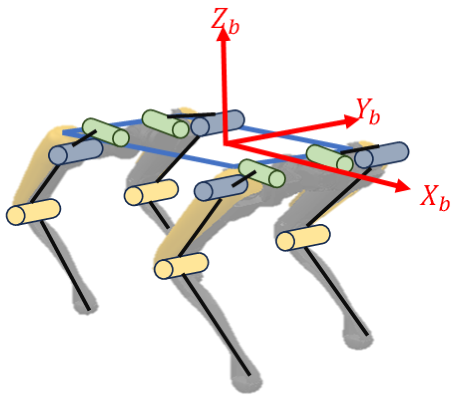
Figure 1 shows the quadruped’s body-fixed coordinate frame and the segmented leg links used throughout this section to derive the forward and inverse kinematics.

The robot used in this study is a quadruped robot modeled after the Spot platform by Boston Dynamics, simulated in CoppeliaSim. The robot has four legs, each with three degrees of freedom (DOF): hip rotation about the x-axis, hip rotation about the y-axis, and knee rotation. The joint limits are specified in

Table 1. Robot joint limits.

Joint	Lower Limit [deg]	Upper Limit [deg]
Hip x	$-45$	45
Hip y	$-80$	100
Knee	$-15$	130

.

The robot is equipped with an inertial measurement unit (IMU) providing orientation, acceleration, and angular velocity data, and force sensors at the leg tips for contact force measurement.

3.1.1. Coordinate Systems and Kinematics

A fixed world frame $\left\{w\right\}$ serves as the inertial reference, and a body frame $\left\{B\right\}$ is attached to the robot at its center of mass (CoM). The robot’s pose is expressed by the vector ${\mathbf{x}}_B={[x_B,y_B,z_B,{\varphi }_B,{\theta }_B,{\psi }_B]}^{\top }$, where $(x_B,y_B,z_B)$ is the position of the body-frame origin in the world frame and $({\varphi }_B,{\theta }_B,{\psi }_B)$ are its roll, pitch, and yaw angles, respectively. Each leg i has three local coordinate systems, $O_{i0}$, $O_{i1}$, and $O_{i2}$, corresponding to the hip-x joint, hip-y joint, and knee joint.

The rotation matrix from the body frame to the world frame is given by:

$${\left[\mathbf{R}\right]}_b^w=R_z\left(\psi \right) · R_y\left(\theta \right) · R_x\left(\varphi \right)$$

(1)

where $R_x$, $R_y$, and $R_z$ are the elementary rotation matrices about the respective axes.

The total transformation matrix is the standard homogeneous transformation matrix representing an element of $SE\left(3\right)$ [29,30]:

$$\mathbf{T}=\left[\begin{array}{cc}{\mathbf{R}}_{3\times 3}& {\mathbf{d}}_{3\times 1}\\ {\mathbf{0}}_{1\times 3}& 1\end{array}\right].$$

(2)

3.1.2. Inverse Kinematics

A geometric approach is used to solve the inverse kinematics for each leg. The solution proceeds in two stages by projecting the leg geometry onto orthogonal planes. Projecting onto the Y-Z plane, the hip-x joint angle $q_1$ is computed as:

$${\alpha }_2=\arcsin \left({\displaystyle \frac{L_1}{\sqrt{y^2+z^2}}}\right),\hspace{1em}{\alpha }_3={\displaystyle \frac{\pi }{2}}-{\alpha }_2$$

(3)

$$q_1={\alpha }_1\mp {\alpha }_3\hspace{1em}(\mathrm{right}/\mathrm{left} \mathrm{leg})$$

(4)

where ${\alpha }_1$ is the angle of the projected leg-tip position vector in the Y-Z plane, measured at the hip-x joint, while ${\alpha }_2$ and ${\alpha }_3$ follow from the lateral hip offset $L_1$; the ∓ sign selects the right or left leg.

Projecting onto the x-$z^{\prime }$ plane, the remaining joint angles are obtained via the law of cosines:

$$B=\sqrt{z_2^2+x_2^2},\hspace{1em}{\beta }_1=\mathrm{atan2}(z_2,x_2)$$

(5)

$${\beta }_2=\arccos \left({\displaystyle \frac{L_2^2+B^2-L_3^2}{2L_{2}B}}\right),\hspace{1em}{\beta }_3=\arccos \left({\displaystyle \frac{L_2^2+L_3^2-B^2}{2L_2{L}_3}}\right)$$

(6)

$$q_2={\beta }_1-{\beta }_2,\hspace{1em}{q}_3=\pi -{\beta }_3$$

(7)

where $L_1$, $L_2$, and $L_3$ are the link lengths of the hip offset, upper leg, and lower leg, respectively.

3.1.3. Static Stability

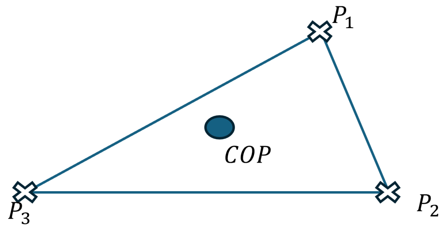
Static stability is maintained by ensuring that the projection of the robot’s CoM lies within the support polygon formed by the grounded feet [31]. This criterion is fundamental to quadruped walking gaits [32,33] and has been extended to footstep planning for multi-legged robots [34]. Before swinging a leg, the robot shifts its CoM so that its horizontal projection moves toward the support polygon centroid ${\mathbf{c}}_{\mathrm{sp}}$ defined by the remaining three grounded legs:

$${\mathbf{c}}_{\mathrm{sp}}=\left[{\displaystyle \frac{1}{3}}{\displaystyle \sum _{i=1}^3}{P}_x^i, {\displaystyle \frac{1}{3}}{\displaystyle \sum _{i=1}^3}{P}_y^i\right]$$

(8)

where $(P_x^i,P_y^i)$ are the horizontal (ground plane) coordinates of the i-th grounded foot. Static stability requires the horizontal CoM projection to lie within the support polygon, so the centroid is expressed in the ground plane. Figure 2 illustrates the support polygon and the CoM projection used for stability verification.

3.1.4. Dynamic Stability During Pushing

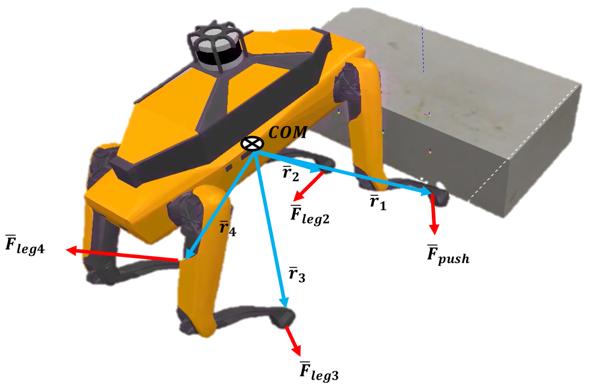
During box-pushing, the robot must maintain dynamic stability under the additional pushing force. Dynamic stability analysis, including zero-moment point (ZMP) methods used in biped walking [35], provides a theoretical basis to ensure that the robot does not tip during contact-rich manipulation. If leg 1 is the pushing leg, the moment balance about the CoM requires:

$${\displaystyle \sum _{i=2}^4}{\mathbf{r}}_i\times {\mathbf{F}}_i+{\mathbf{r}}_1\times {\mathbf{F}}_{\mathrm{push}}=\mathbf{0}$$

(9)

where ${\mathbf{r}}_i$ denotes the position vector of leg i relative to the CoM, ${\mathbf{F}}_i$ the ground reaction force at leg i, and ${\mathbf{F}}_{\mathrm{push}}$ the reaction force from the box. Figure 3 illustrates the force balance during a pushing action. In practice, dynamic stability is encouraged through a penalty in the RL reward function that discourages configurations in which the robot tips over; this biases the policy toward stable behavior but does not impose a hard stability constraint. As a quantitative cross-check, the trunk pitch and roll angles were monitored throughout every reported rollout and stayed within $\pm 5°$ in the straight-line pushing experiments and within $\pm 8°$ during the higher-curvature circular pushes; no rollout was terminated by the fall criterion of Section 3.3.5. The trunk-angle margin therefore replaces a closed-form ZMP trace as the practical stability metric reported here, and we note that closed-form ZMP or capture-point checks would be a natural next step before sim-to-real transfer.

3.2. RRT-Based Motion Planning

The RRT algorithm is used for global path planning from the robot’s initial position to the target object. The algorithm incrementally builds a tree $\mathcal{T}$ by sampling random configurations $q_{\mathrm{rand}}$—with goal biasing that draws the goal configuration $q_{\mathrm{goal}}\in \mathcal{G}$ with probability $p_{\mathrm{goal}}$—and extending the nearest node $q_{\mathrm{near}}$ toward $q_{\mathrm{rand}}$, subject to collision constraints. Each node stores a pointer to its parent. Once a newly added node lands in the goal region $\mathcal{G}$, the tree is connected to $q_{\mathrm{goal}}$, and the final path is recovered by following parent pointers from $q_{\mathrm{goal}}$ back to $q_{\mathrm{start}}$. Algorithm 1 summarizes the procedure.

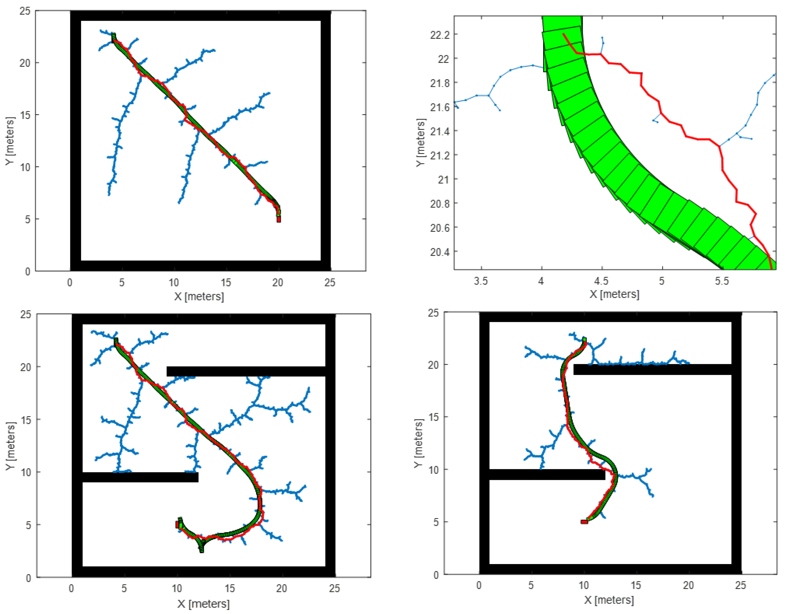
Figure 4 illustrates the RRT tree expansion process, showing how the algorithm incrementally explores the configuration space by extending branches toward randomly sampled points.

Algorithm 1 RRT Path Planning for the Quadruped Robot

1: Input: start $q_{\mathrm{start}}$; goal region $\mathcal{G}$ with goal configuration $q_{\mathrm{goal}}\in \mathcal{G}$; obstacle map $\mathcal{O}$; goal-bias probability $p_{\mathrm{goal}}$   2: Output: Path $\mathcal{P}=\{q_0,q_1,\dots ,q_n\}$   3: $\mathcal{T}\leftarrow \left\{q_{\mathrm{start}}\right\}$; $\mathrm{parent}\left(q_{\mathrm{start}}\right)\leftarrow ⌀$   4: while $q_{\mathrm{goal}}\notin \mathcal{T}$ do   5:     if Rand() $<p_{\mathrm{goal}}$ then   6:         $q_{\mathrm{rand}}\leftarrow q_{\mathrm{goal}}$                                 ▹ goal biasing   7:     else   8:         $q_{\mathrm{rand}}\leftarrow$ SampleRandom()   9:     end if 10:     $q_{\mathrm{near}}\leftarrow$ NearestNode($\mathcal{T}$, $q_{\mathrm{rand}}$) 11:     $q_{\mathrm{new}}\leftarrow$ Steer($q_{\mathrm{near}}$, $q_{\mathrm{rand}}$) 12:     if CollisionFree($q_{\mathrm{near}}$, $q_{\mathrm{new}}$, $\mathcal{O}$) then 13:         $\mathcal{T}.\mathrm{add}\left(q_{\mathrm{new}}\right)$; $\mathrm{parent}\left(q_{\mathrm{new}}\right)\leftarrow q_{\mathrm{near}}$ 14:         if $q_{\mathrm{new}}\in \mathcal{G}$ and CollisionFree($q_{\mathrm{new}}$, $q_{\mathrm{goal}}$, $\mathcal{O}$) then 15:              $\mathcal{T}.\mathrm{add}\left(q_{\mathrm{goal}}\right)$; $\mathrm{parent}\left(q_{\mathrm{goal}}\right)\leftarrow q_{\mathrm{new}}$ 16:         end if 17:     end if 18: end while 19: $\mathcal{P}\leftarrow$ExtractPath($\mathcal{T}$, $q_{\mathrm{start}}$, $q_{\mathrm{goal}}$)                        ▹ via parent pointers 20: $\mathcal{P}\leftarrow$SmoothPath($\mathcal{P}$) 21: return $\mathcal{P}$

3.2.1. Path Smoothing

The raw RRT path may contain sharp turns that are kinematically infeasible for the robot. Path smoothing is applied using MATLAB R2023a’s (The MathWorks, Inc., Natick, MA, USA) Robotics System Toolbox, which employs spline interpolation to fit smooth curves between waypoints. In open environments, the smoothing window is constrained to remain within the clearance of the original collision-free waypoints, so the smoothed path is guaranteed to lie in the same free-space tube as the raw RRT path, and feasibility is preserved without further checks. For cluttered environments, the same pipeline is extended by an explicit re-verification step: the smoothed path is densely re-sampled, and each sample is tested against the obstacle map; if any sample is in collision, the smoothing window is shrunk locally and the spline is refitted, repeating until the smoothed path is collision-free or the window collapses back to the raw RRT polyline. The open-environment results reported here did not require this fall-back; documenting it explicitly closes the gap noted in the original submission.

3.2.2. Adaptation to Robot Geometry

To map the planned path to the physical robot, the robot is represented as a rectangle viewed from above, where the center corresponds to the planned trajectory waypoint and each corner represents a leg. As the rectangle moves along the smoothed path, the displacement of each corner defines the stepping motion for the corresponding leg, using parabolic swing trajectories parameterized by displacement $(dx,dy)$ and step height h. The swing leg trajectory parameters are summarized in

Table 2. Swing leg trajectory parameters.

Parameter	Symbol	Description
Displacement x	$dx$	Horizontal displacement in the x-direction
Displacement y	$dy$	Horizontal displacement in the y-direction
Step height	h	Maximum height of the parabolic swing arc
Swing duration	$T_{\mathrm{swing}}$	Time allocated for the swing phase

.

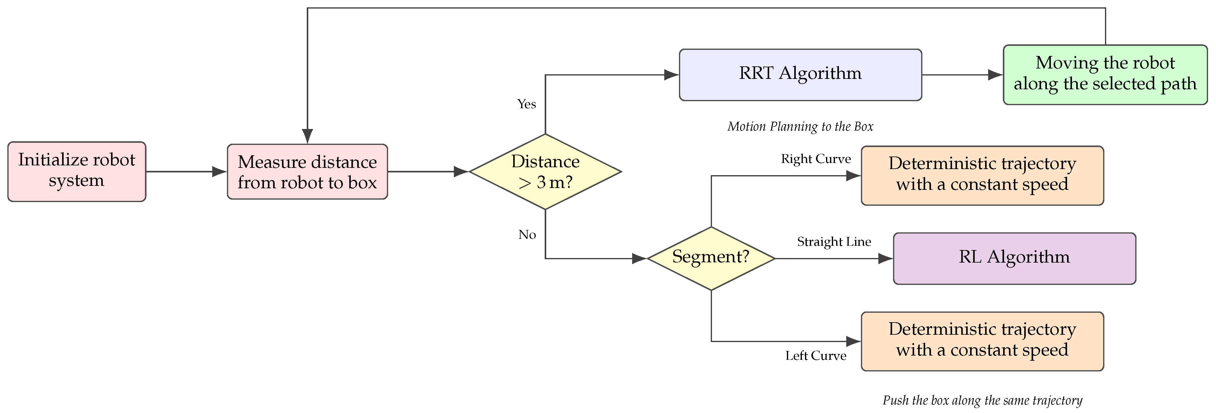
Figure 5 gives the overall control flow that links these components: the RRT planner guides the robot toward the box, and control is handed over to the reinforcement learning pushing policy once the robot is close enough to the box.

The 3 m switching distance was selected as a geometric upper bound on the radius of the contact-pushing workspace: at distances greater than this radius, the robot is outside the box’s immediate vicinity and locomotion errors dominate the cost-to-go, whereas inside this radius, the residual approach error is small enough that the learned Bézier pushing primitive can correct it. We did not perform a formal sensitivity analysis of the threshold value; this is left as future work. We expect performance to be relatively insensitive to the exact value as long as the threshold is larger than the cumulative position error built up during locomotion and smaller than the planner’s average inter-waypoint spacing, so that the RL agent is engaged neither too early (with the box still out of reach) nor too late (when the robot has already overshot).

3.3. Reinforcement Learning for Object Manipulation

3.3.1. Background

Reinforcement learning is a framework in which an agent learns to make sequential decisions by interacting with an environment to maximize a cumulative reward signal [9,10]. The agent selects actions according to a policy, which can be stochastic, $\pi \left(a\right|s)$, representing the probability of choosing action a in state s, or deterministic, $a=\pi \left(s\right)$ [36,37]. The agent’s objective is to maximize the expected return, defined as the discounted cumulative reward:

$$G_t={\displaystyle \sum _{k=0}^{\infty }}{\gamma }^k{R}_{t+k+1}$$

(10)

where $\gamma \in [0,1]$ is the discount factor controlling the trade-off between immediate and future rewards [9]. The state-value function $V_{\pi }\left(s\right)$ and action-value function $Q_{\pi }(s,a)$ quantify the expected return from a given state or state–action pair under policy $\pi$:

$$V_{\pi }\left(s\right)={\mathbb{E}}_{\pi }\left[G_t\mid s_t=s\right]$$

(11)

$$Q_{\pi }(s,a)={\mathbb{E}}_{\pi }\left[G_t\mid s_t=s,a_t=a\right]$$

(12)

These foundational concepts underpin the deep RL algorithms—such as DQN [17] and policy gradient methods [36]—that have achieved remarkable success in complex control tasks.

3.3.2. Proximal Policy Optimization

PPO [11] is a policy gradient method that optimizes a clipped surrogate objective to prevent excessively large policy updates. The objective function is:

$$L^{\mathrm{CLIP}}\left(\theta \right)={\widehat{\mathbb{E}}}_t\left[\min \left(r_t\left(\theta \right){\widehat{A}}_t, \mathrm{clip}(r_t\left(\theta \right),1-ϵ,1+ϵ){\widehat{A}}_t\right)\right]$$

(13)

where $r_t\left(\theta \right)={\pi }_{\theta }\left(a_t\right|s_t)/{\pi }_{{\theta }_{\mathrm{old}}}\left(a_t\right|s_t)$ is the probability ratio between the new and old policies, ${\widehat{A}}_t$ is the estimated advantage, and $ϵ$ is the clipping parameter. This formulation ensures stable training by constraining the magnitude of the policy update.

3.3.3. Bézier Curve Leg Trajectories

A key contribution of this work is the parameterization of the pushing leg trajectory using Bézier curves. A Bézier curve of degree n is defined by:

$$\mathbf{B}\left(t\right)={\displaystyle \sum _{i=0}^n}\left({\displaystyle \genfrac{}{}{0pt}{}{n}{i}}\right){(1-t)}^{n-i}{t}^i{\mathbf{P}}_i,\hspace{1em}t\in [0,1]$$

(14)

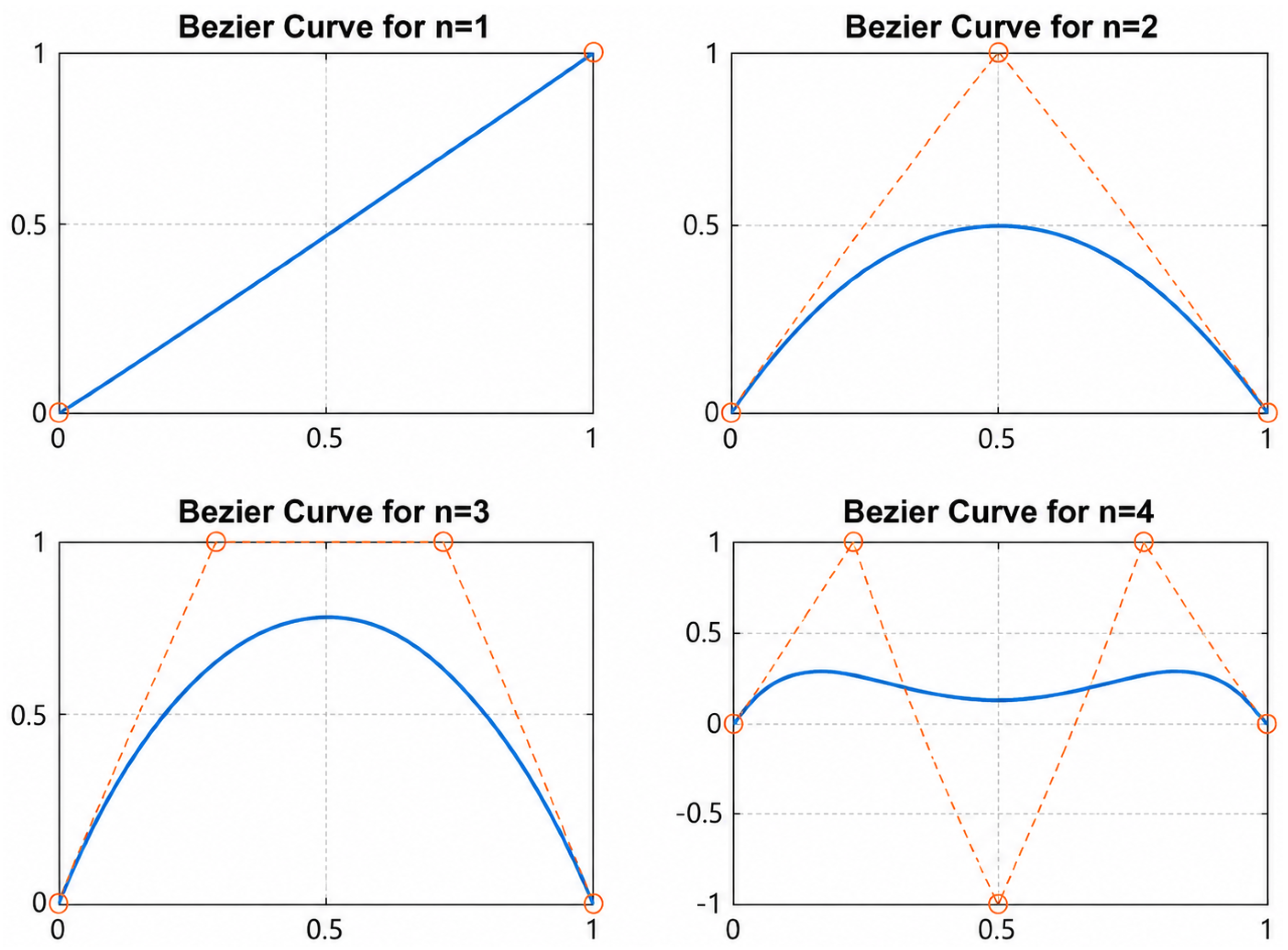
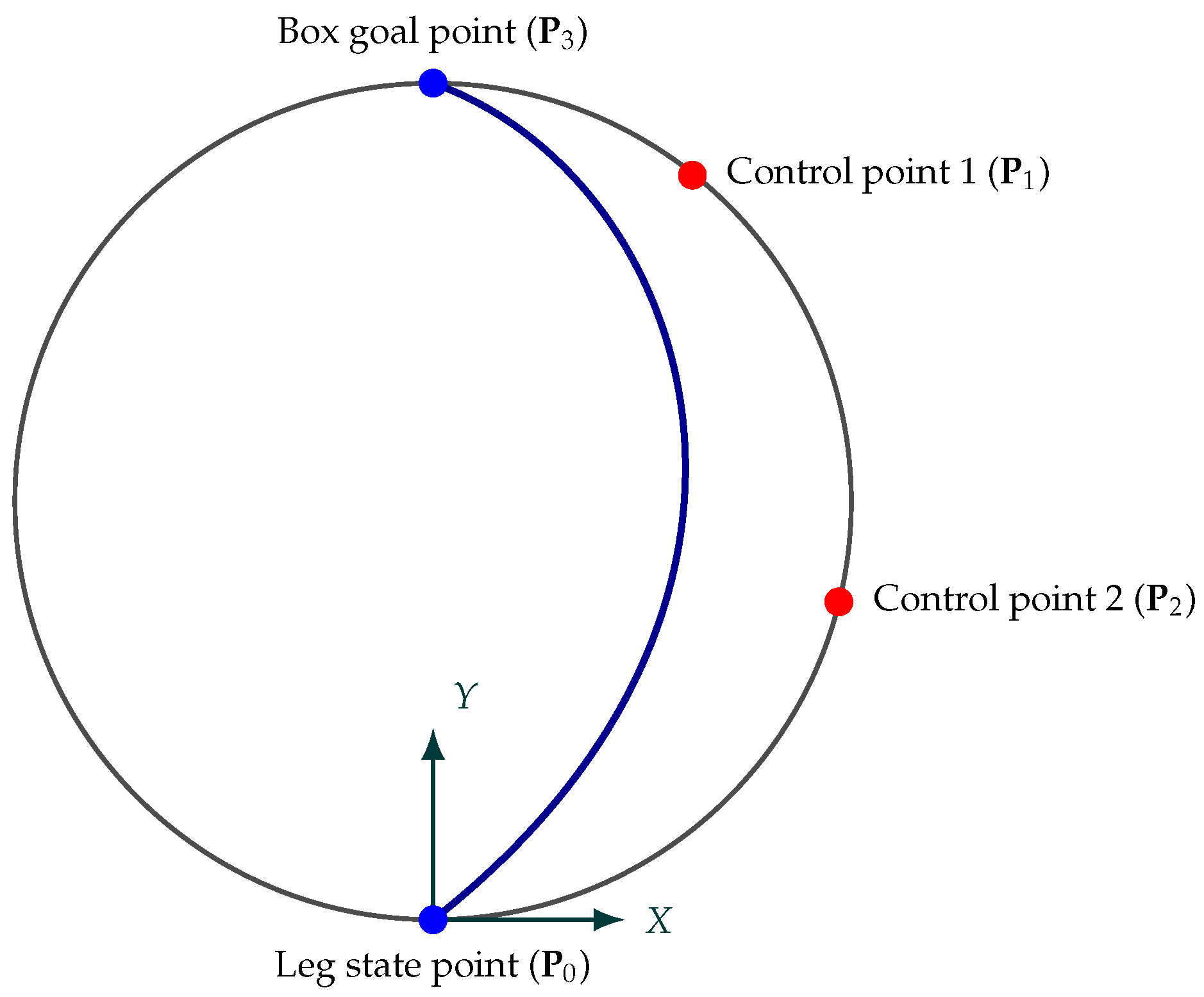
where ${\mathbf{P}}_i$ are the control points. Figure 6 illustrates Bézier curves of increasing degree together with their control points and control polygons. In this work, cubic Bézier curves ($n=3$) are used, with the start point ${\mathbf{P}}_0$ set to the current leg-tip position, the end point ${\mathbf{P}}_3$ set to the contact point on the box, and two intermediate control points ${\mathbf{P}}_1$ and ${\mathbf{P}}_2$ determined by the RL agent’s actions. The positions of ${\mathbf{P}}_1$ and ${\mathbf{P}}_2$ are determined by two scalar values $w_1,w_2\in [0,1]$ output by the agent. As illustrated in Figure 7, the two intermediate control points lie on a circular locus passing through the leg tip ${\mathbf{P}}_0$ and the contact point ${\mathbf{P}}_3$; each scalar $w_i$ selects the position of control point ${\mathbf{P}}_i$ along this locus. Concretely, let $\mathbf{M}=\frac{1}{2}({\mathbf{P}}_0+{\mathbf{P}}_3)$ be the chord midpoint and $\mathbf{n}$ the in-plane unit normal to the chord ${\mathbf{P}}_0{\mathbf{P}}_3$ (pointing in the upward swing direction). Each intermediate control point is then placed on a circular locus of radius $r=\frac{1}{2}\parallel {\mathbf{P}}_3-{\mathbf{P}}_0\parallel$ centered at $\mathbf{M}$ according to the affine map

$${\mathbf{P}}_i = \mathbf{M}+r \left[\sin \left({\theta }_i\right) \widehat{\mathbf{u}}+\cos \left({\theta }_i\right) \mathbf{n}\right],\hspace{1em}\hspace{1em}{\theta }_i = {\theta }_{\min }+w_i ({\theta }_{\max }-{\theta }_{\min }),\hspace{1em}\hspace{1em}i\in \{1,2\},$$

(15)

with $\widehat{\mathbf{u}}$ the unit vector along the chord from ${\mathbf{P}}_0$ to ${\mathbf{P}}_3$ and a fixed angular range $[{\theta }_{\min },{\theta }_{\max }]=[0,\pi ]$ that brackets the swing-side half-circle. Thus, $w_1$ and $w_2$ jointly set the curvature and approach angle of the pushing trajectory: small $w_i$ places ${\mathbf{P}}_i$ close to the chord (a low, shallow push), while large $w_i$ lifts ${\mathbf{P}}_i$ high above the chord (a steep approach). The numerical values used in the experiments are also provided with the released source code (Data Availability Statement) for full reproducibility.

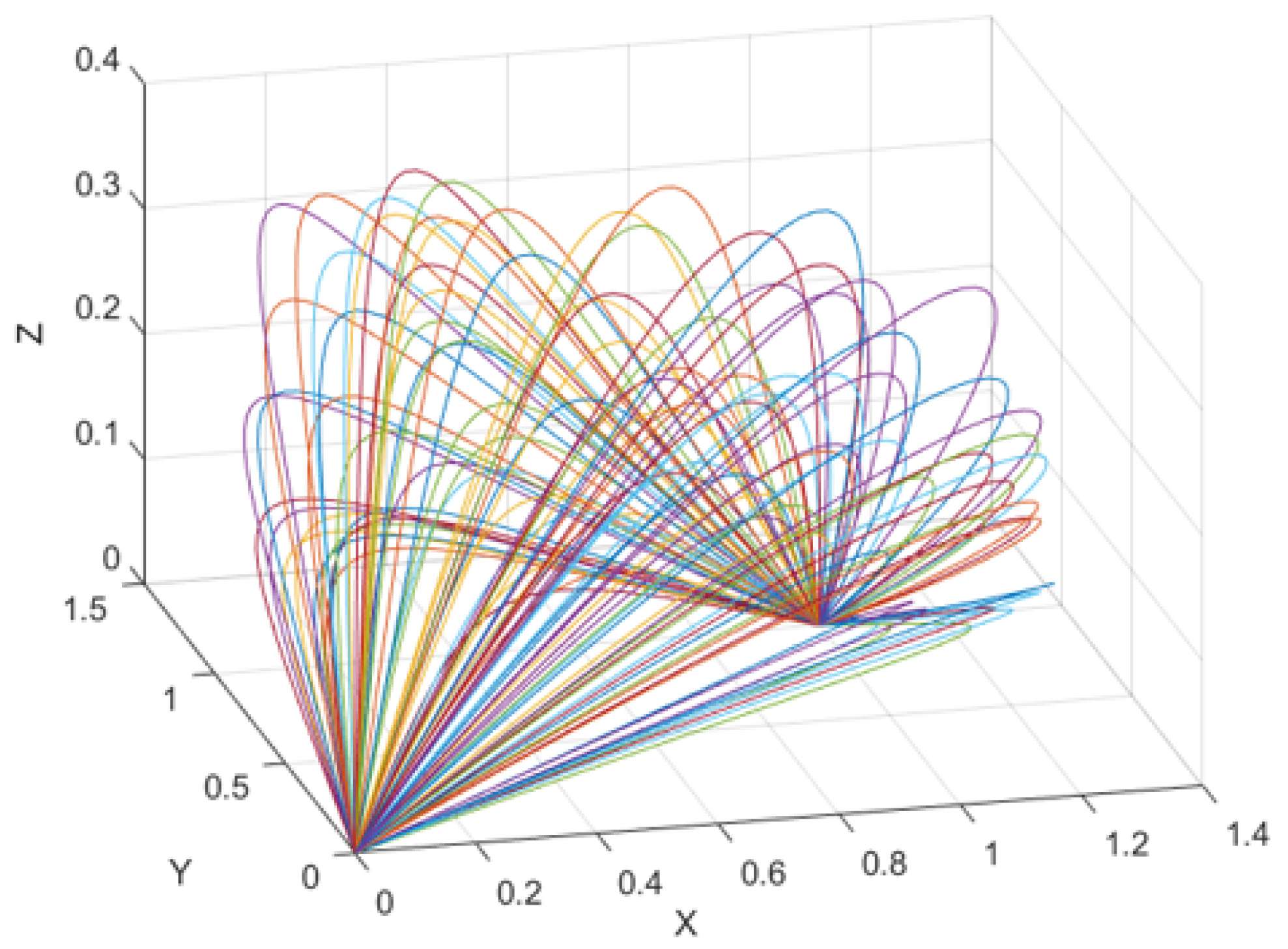
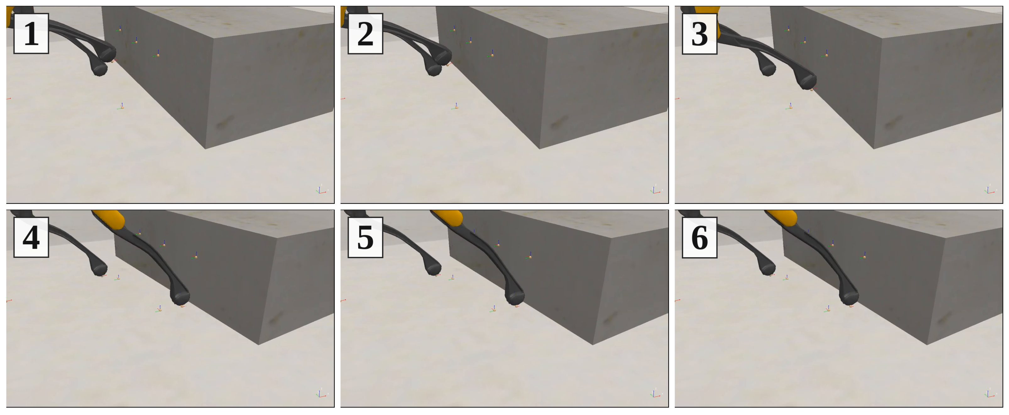
This parameterization offers several advantages: (1) inherent smoothness of the resulting trajectory, (2) a compact action space for the RL agent, and (3) intuitive control over the approach angle and contact dynamics. Figure 7 shows a schematic of the Bézier construction, and Figure 8 shows the resulting family of candidate leg trajectories. The Bézier curve parameters are listed in

Table 3. Bézier curve trajectory parameters for box pushing.

Parameter	Description
${\mathbf{P}}_0$ (start point)	Current position of the pushing leg tip
${\mathbf{P}}_3$ (end point)	Target contact point on the box surface
${\mathbf{P}}_1,{\mathbf{P}}_2$ (control points)	Intermediate control points; each positioned by one scalar action
$w_1\in [0,1]$	Scalar action positioning control point ${\mathbf{P}}_1$
$w_2\in [0,1]$	Scalar action positioning control point ${\mathbf{P}}_2$

.

3.3.4. Reward Function Design

A well-designed reward function is critical to guide the RL agent toward the desired behavior. In many manipulation tasks, a sparse reward signal—such as a binary success or failure flag upon task completion—provides insufficient feedback for the agent to learn efficiently. We therefore incorporate additional intermediate reward components that provide denser feedback throughout each episode. In this work, the reward function is decomposed into a position component that penalizes the distance between the box and its target, an angular component that penalizes orientation misalignment, and a stability penalty that discourages the robot from tipping over. These components collectively guide the agent to discover pushing strategies that are both accurate and stable.

The reward function is designed to encourage the agent to push the box toward the target while maintaining robot stability. It comprises three components:

$$R_t=r_{\mathrm{position}}+r_{\mathrm{angle}}-10 · {⊮}_{\mathrm{fall}}$$

(16)

where ${⊮}_{\mathrm{fall}}$ is an indicator function that equals 1 when the robot falls. The position and angular components are:

$$r_{\mathrm{position}}=-10 · \sqrt{e_1+e_2}$$

(17)

$$r_{\mathrm{angle}}=-2 · \sqrt{e_{\mathrm{angle}}}$$

(18)

where $e_1={\parallel {\mathbf{p}}_{\mathrm{target}}^{c_1}-{\mathbf{p}}_{\mathrm{box}}^{c_1}\parallel }^2$ and $e_2={\parallel {\mathbf{p}}_{\mathrm{target}}^{c_2}-{\mathbf{p}}_{\mathrm{box}}^{c_2}\parallel }^2$ are the squared position errors of the two tracked box corners, and $e_{\mathrm{angle}}={({\theta }_{\mathrm{target}}-{\theta }_{\mathrm{box}})}^2$ is the squared angular error between the box and target orientations. With these definitions, $r_{\mathrm{angle}}=-2 |{\theta }_{\mathrm{target}}-{\theta }_{\mathrm{box}}|$ and $r_{\mathrm{position}}$ aggregates the two corner distances into a single positional penalty. Figure 9 shows a representative close-up of a single Bézier-parameterized leg swing contacting and pushing the box face in the simulation.

3.3.5. Episode Definition, Termination, and Reset

Each training episode comprises up to $T_{\max }=200$ environment interactions between the PPO agent and the simulator, where one interaction corresponds to one Bézier leg-swing-and-push cycle (Section 3.3.3). Within each interaction, the simulator advances the physics until the swing completes, so a single PPO step subsumes a multi-step internal simulator integration; this is the unit at which the state transition $s_t\to s_{t+1}$ (Section 4.4) is sampled. An episode terminates when any of the following conditions is met: (i) the box centroid reaches within a positional tolerance of the target pose and the orientation error is below the angular tolerance (task success); (ii) the robot tips over, as detected by the trunk pitch or roll exceeding the stability threshold used to compute the fall penalty in Equation (16); or (iii) the maximum step count $T_{\max }$ is reached without success (timeout). On termination, the simulation scene is reset by restoring the robot, box, and target markers to a fixed reference configuration; the random seed for the next episode is incremented; and the agent buffers continue accumulating transitions for the next on-policy update.

4. Implementation

4.1. Simulation Environment

The simulation environment is built using CoppeliaSim EDU 4.5 (Coppelia Robotics AG, Zurich, Switzerland) (formerly V-REP) [38] with the MuJoCo physics engine. CoppeliaSim provides a versatile robotics simulation framework, while MuJoCo ensures accurate rigid-body dynamics and contact simulation. The simulation is controlled externally via Python using the ZeroMQ remote API [39], which enables synchronous stepping of the simulation and retrieval of sensor data.

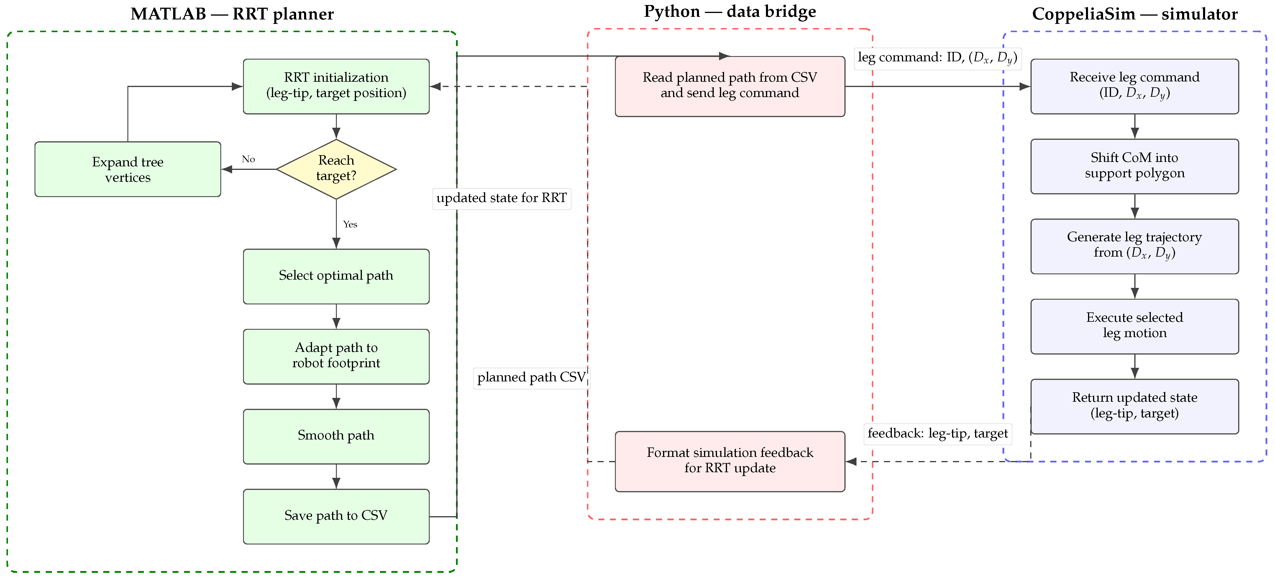
The architecture integrates three software components (Figure 10): CoppeliaSim handles the physics simulation and visualization, MATLAB (R2023a) performs RRT path planning and path smoothing using the Robotics System Toolbox, and Python (3.10.11; Python Software Foundation, Wilmington, DE, USA) trains the RL agent using Stable Baselines3 v1.8.0 [40] within a custom OpenAI Gym environment [41].

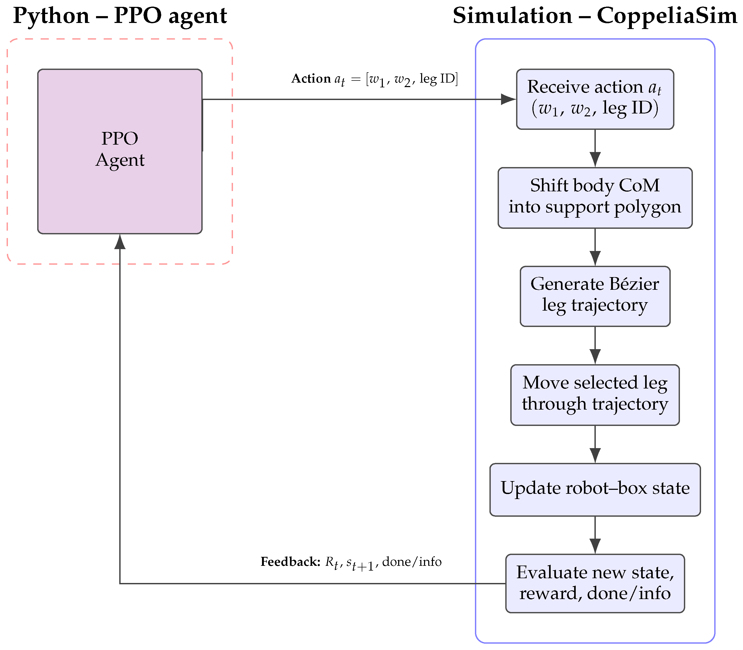
The RL training loop operates within the CoppeliaSim environment as shown in Figure 11. At each step, the Python agent observes the current state $s_t$, samples an action $a_t=[w_1,w_2,\mathrm{leg} \mathrm{ID}]$ from the current policy (updated during training and fixed during evaluation), and sends the corresponding Bézier control parameters to CoppeliaSim. The simulator carries the chain through trajectory generation and execution, then evaluates the resulting box–robot state to produce the next observation $s_{t+1}$, the scalar reward $R_t$, and a step-completion flag, which are returned to the agent.

4.2. Network Architecture

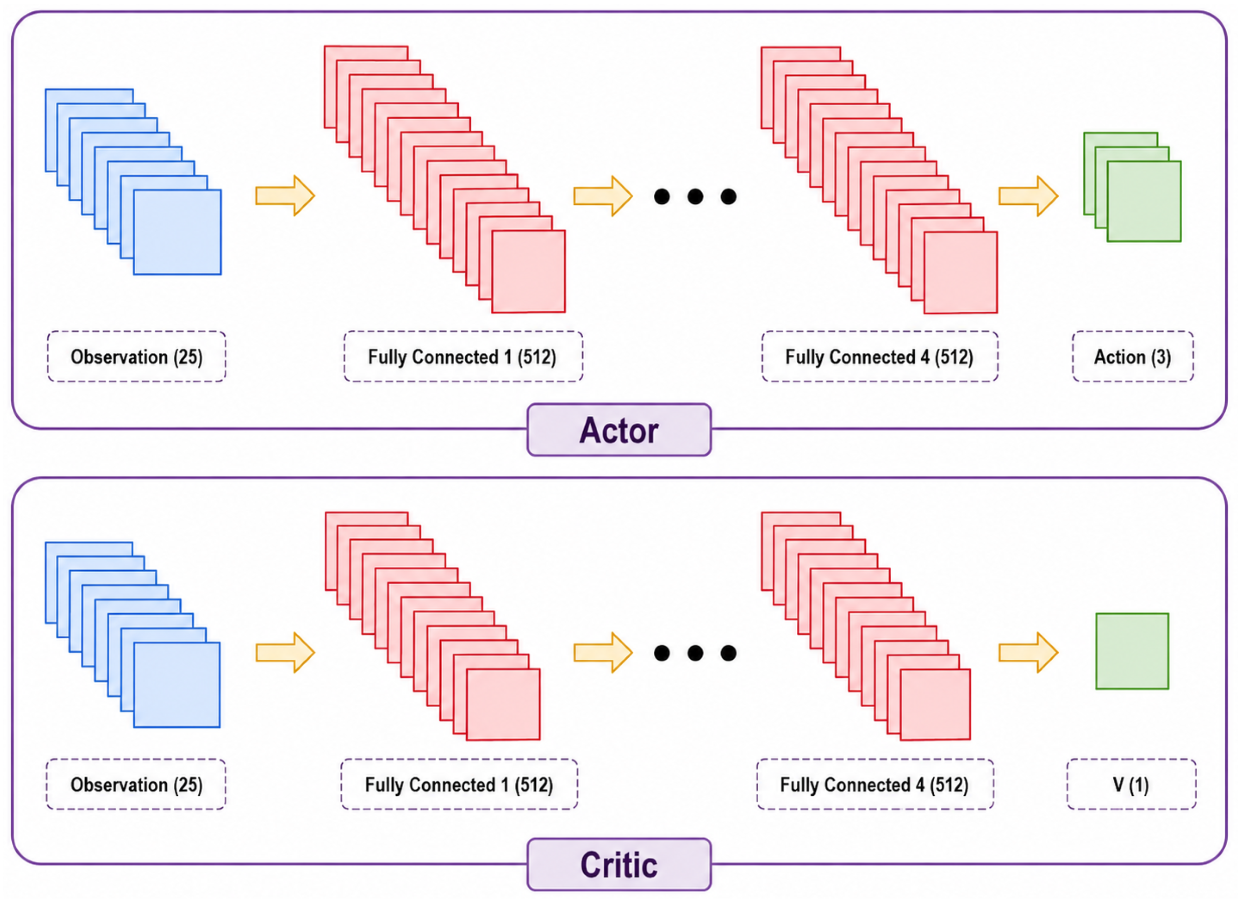
The actor–critic network architecture used for PPO is shown in Figure 12. Both the actor (policy) and critic (value) networks use the same architecture: four fully connected hidden layers with 512 neurons each and ReLU activation functions. This size was selected pragmatically rather than through a formal ablation: it is consistent with the Stable-Baselines3 PPO defaults for continuous control tasks and gave stable training across the configurations explored, while comfortably fitting on a single workstation GPU. We acknowledge that a network with ∼${10}^6$ parameters is likely larger than strictly necessary for this low-dimensional pushing task; a width and depth ablation (e.g., $4\times 64$, $2\times 128$) is left as future work, and we expect substantially smaller networks to reach comparable performance once the action space is the only learned component. The policy network outputs the action mean vector—three-dimensional in the fixed entry value configuration or four-dimensional when the push depth is additionally learned—while the critic network outputs a scalar value estimate $V\left(s_t\right)$. The leg-selection component is produced as a continuous output and discretized to the nearest leg index (Section 4.4). Because only two legs are eligible, the leg-selection output reduces to thresholding a single scalar at its midpoint, which is mathematically equivalent to a binary categorical choice and therefore preserves a single decision boundary rather than several quantization bins. We deliberately kept the scalar form so that the action distribution remains a single multivariate Gaussian over $(w_1,w_2,\mathcal{l})$ and, where used, d; this avoids the engineering overhead of a hybrid continuous–categorical policy head while reproducing the categorical decision exactly through the midpoint threshold. Section 4.4 restates this mapping.

The training hyperparameters are listed in

Table 4. Key training hyperparameters for the PPO agent.

Hyperparameter	Value	Description
Learning rate ($\alpha$)	0.001	Gradient descent step size
Batch size	512	Samples per gradient update
Discount factor ($\gamma$)	0.99	Future reward weighting

.

Unless otherwise noted, the remaining PPO hyperparameters (e.g., the clipping parameter $ϵ$, the GAE parameter $\lambda$, the number of optimization epochs per update, and the rollout length) were left at the Stable-Baselines3 PPO defaults. Because these defaults can depend on the library version, the specific Stable-Baselines3 version and the complete set of hyperparameters are provided with the released training scripts (see the Data Availability Statement) to ensure reproducibility.

4.3. State Transition Dynamics

The environment state at PPO step t is $s_t=(s_t^{\mathrm{robot}},s_t^{\mathrm{box}},s_t^{\mathrm{goal}})$, comprising the robot pose, the box pose, and the goal pose (Section 4.4). State transitions are produced by CoppeliaSim’s built-in rigid-body simulator: given an action $a_t$, CoppeliaSim integrates the contact and rigid-body dynamics for the duration of the commanded Bézier leg swing at the simulator’s default time step, then returns the post-swing pose of the robot and the box. The next observation $s_{t+1}$ is read directly from the simulator’s pose channels; there is no analytical box model overlaid on the simulator. As a consequence, the transition operator implements precisely the contact mechanics that CoppeliaSim provides, with the limitations (friction model and contact stiffness) inherited from that simulator.

4.4. Observation and Action Spaces

The observation space is a 25-dimensional vector comprising:

$$\mathbf{o}={\left[ {\mathbf{p}}_{\mathrm{body}}^{\left(3\right)}, {\mathbf{p}}_{\mathrm{box}}^{c_1\left(3\right)}, {\mathbf{p}}_{\mathrm{box}}^{c_2\left(3\right)}, {\mathbf{p}}_{\mathrm{tips}}^{\left(12\right)}, {\mathbf{p}}_{\mathrm{target}}^{c_1\left(2\right)}, {\mathbf{p}}_{\mathrm{target}}^{c_2\left(2\right)} \right]}^{\top }\in {\mathbb{R}}^{25}$$

(19)

where ${\mathbf{p}}_{\mathrm{body}}$ is the body position, ${\mathbf{p}}_{\mathrm{box}}^{c_i}$ are two box-corner positions, ${\mathbf{p}}_{\mathrm{tips}}$ are the four leg-tip positions, and ${\mathbf{p}}_{\mathrm{target}}^{c_i}$ are two target-corner positions, all in world coordinates.

The action space is a three-dimensional vector:

$${\mathbf{a}}_t=[ w_1, w_2, \mathcal{l} ]$$

(20)

where $w_1,w_2\in [0,1]$ are the Bézier control-point parameters (Section 3.3.3) and ℓ selects one of the two front legs for pushing. The leg index is obtained by mapping the continuous policy output ℓ to the nearest of the two discrete indices $\{1,2\}$. In the variable entry value configuration (Section 5.2), a fourth component $d\in [0,1]$ encoding the normalized push depth (entry value) is appended, yielding a four-dimensional action vector.

5. Results

5.1. Motion Planning with RRT

The RRT algorithm was applied to plan collision-free paths from the robot’s starting position to the box location across the representative occupancy maps illustrated in Figure 4. The planned paths were smoothed and adapted to the robot’s rectangular footprint, with each corner trajectory corresponding to an individual leg’s stepping sequence. The motion planning transfers effectively from the MATLAB planning environment to the physics simulation; the executed CoppeliaSim trajectory and the planned MATLAB path are compared qualitatively in Figure 13, while a quantitative tracking-error metric was not computed in this study.

5.2. Straight-Line Box Pushing

The PPO agent was trained to push a box in a straight line from its initial position to a target location. The two conditions below differ in whether the entry value—a commanded contact-depth parameter that sets how far the leg tip travels toward the box surface along the Bézier trajectory during a push—is held fixed or learned as an additional action:

5.2.1. Fixed Entry Value

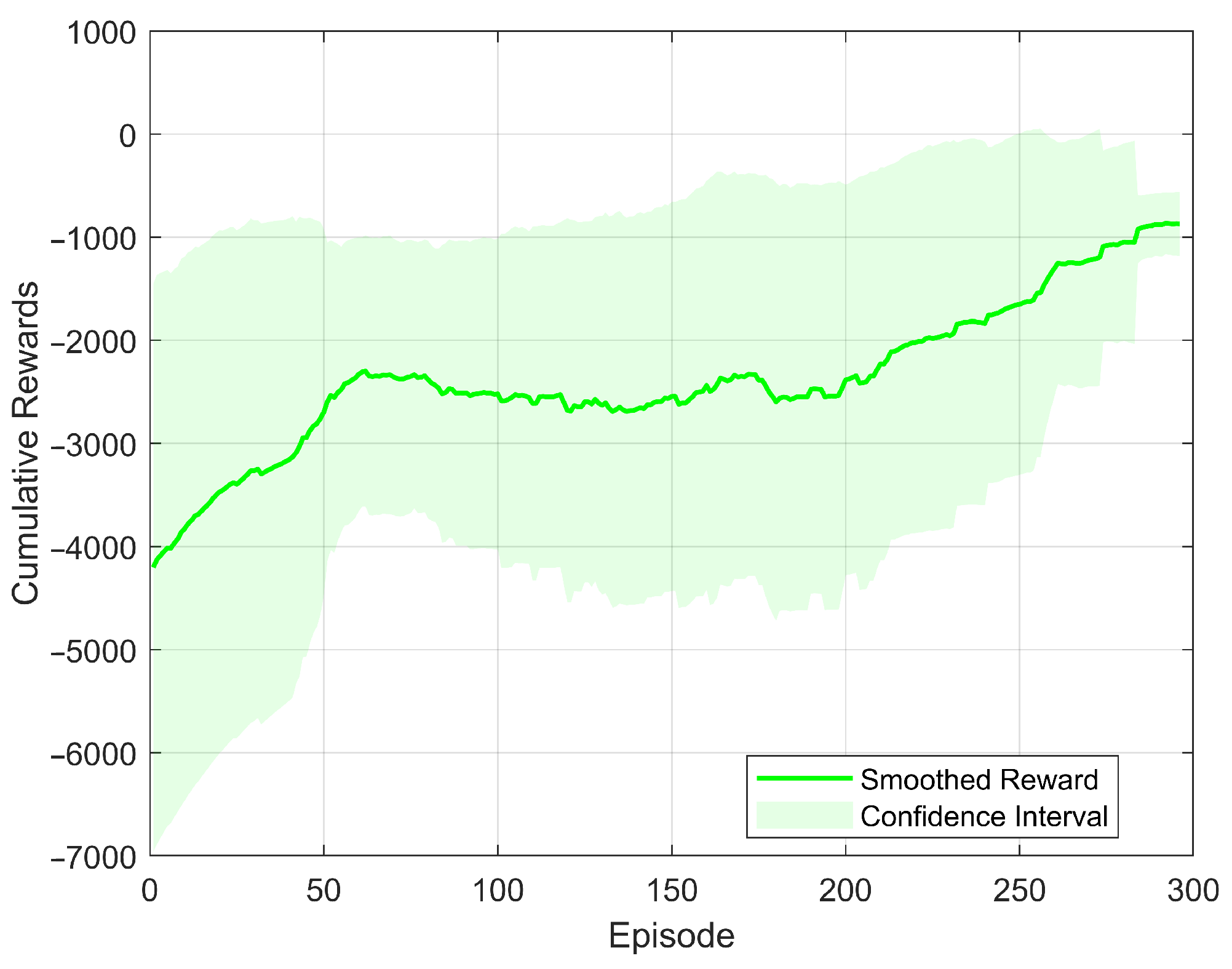
In this configuration, the depth of the leg push into the box is fixed, and the agent learns only the Bézier curve parameters and leg selection. The learning curve (Figure 14) shows that cumulative rewards start negative, increase sharply over the first 50 episodes, and stabilize thereafter, indicating that the policy settles on an effective pushing behavior. The narrowing confidence interval reflects increasingly consistent performance.

5.2.2. Variable Entry Value

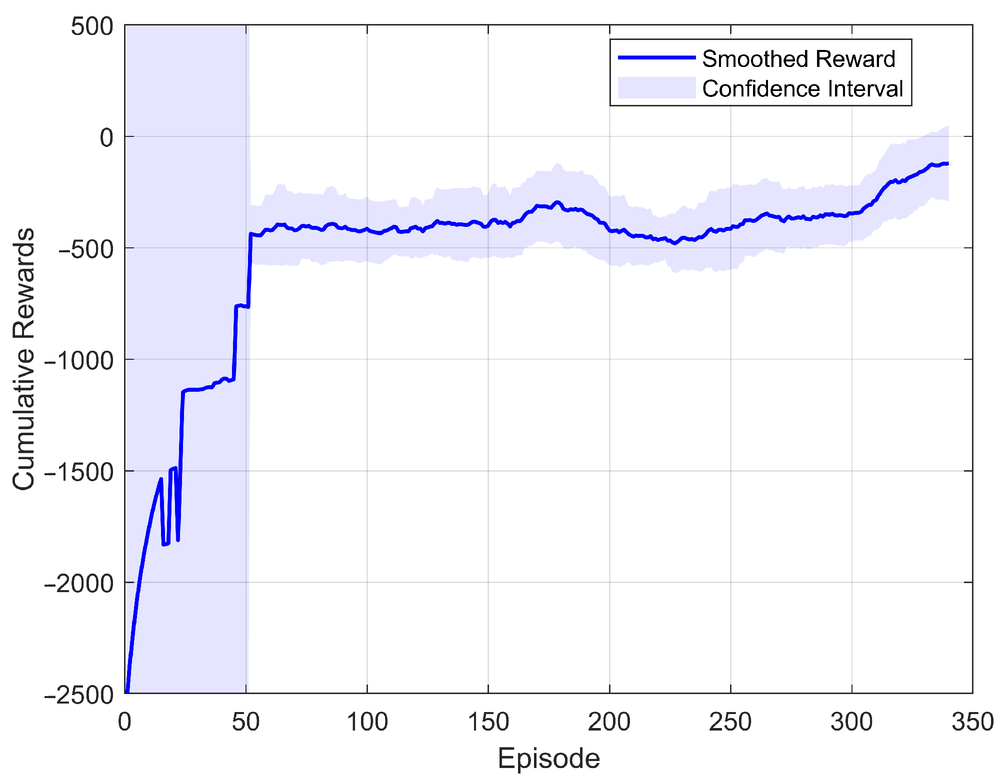
Here, the agent additionally controls the push depth as a fourth action dimension. Despite the increased complexity, the agent still learns to push the box in a straight line (Figure 15), indicating that the PPO-based approach with Bézier curve parameterization scales to the larger action space.

5.3. Generalization Analysis

To evaluate the robustness of the trained agent, we tested it with box masses ranging from the training mass (0.1 kg) to significantly higher values. The analysis examines both angular and position errors as functions of box mass.

The results (Figure 16) show that the agent, trained on a 0.1 kg box, continues to push the box toward the target as its mass increases over the tested range (up to eight times the training mass): the position and angular errors increase with added mass, following the fitted trends in Figure 16 rather than diverging. This analysis varied only the box mass; object shape, friction, and surface conditions were held constant and are discussed among the limitations in Section 6.

5.4. Straight-Line Pushing Illustration

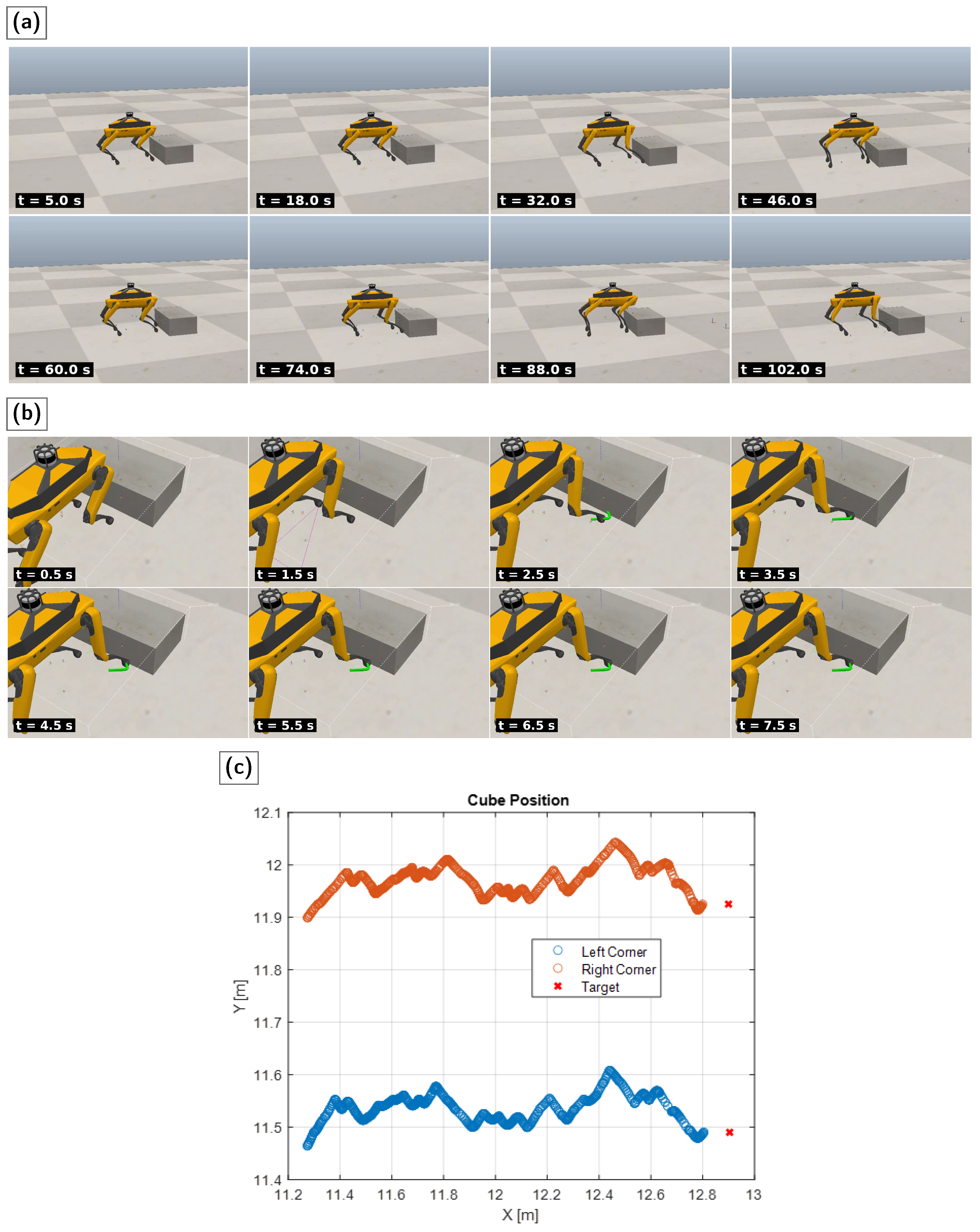
Figure 17 illustrates the robot pushing a box in a straight line using the trained agent and the resulting box-corner trajectory.

Figure 17 pairs the qualitative view of the push with the quantitative box-corner trajectory; the box follows an approximately straight path with some residual lateral deviation from the targets.

5.5. Circular Path Pushing

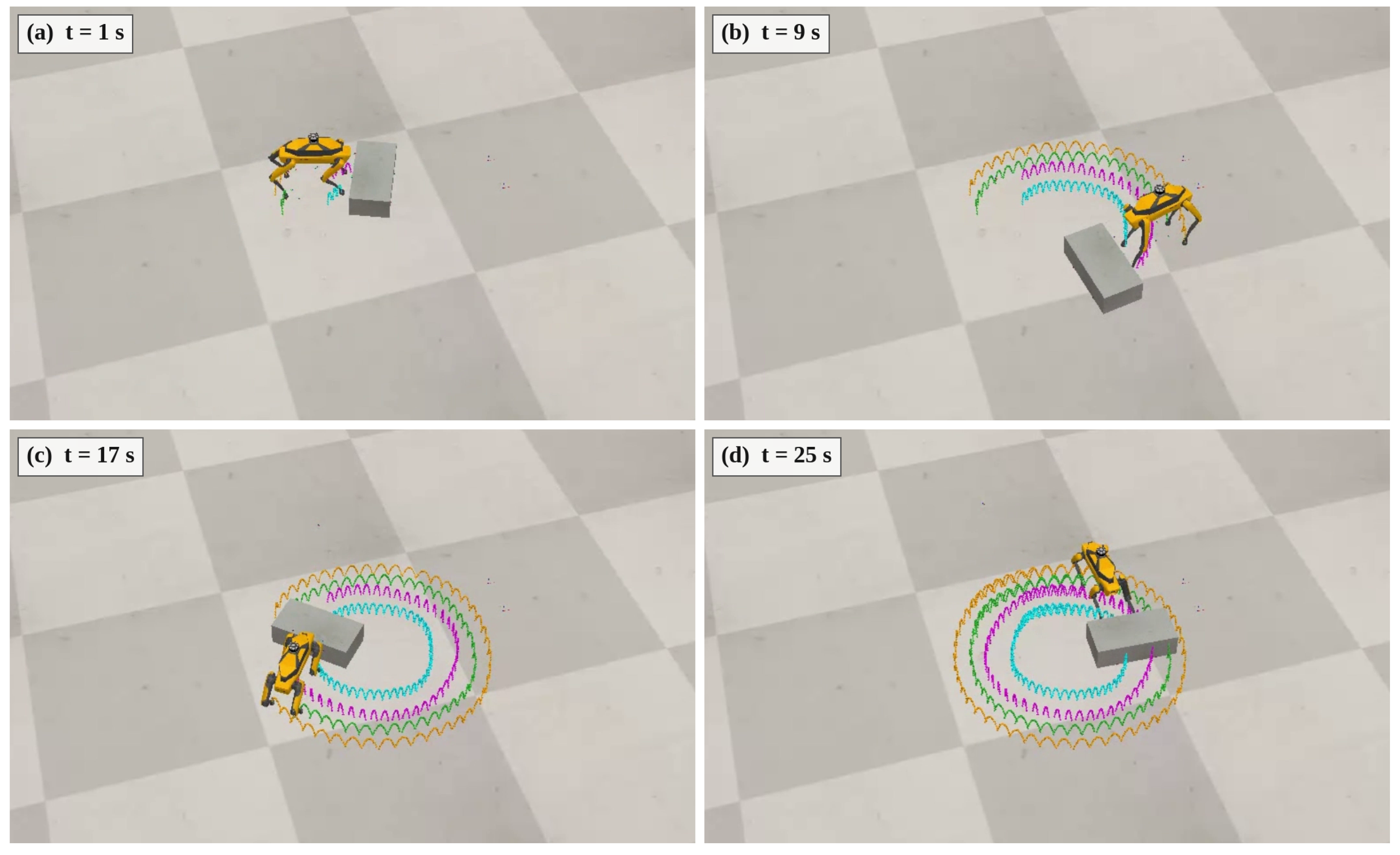
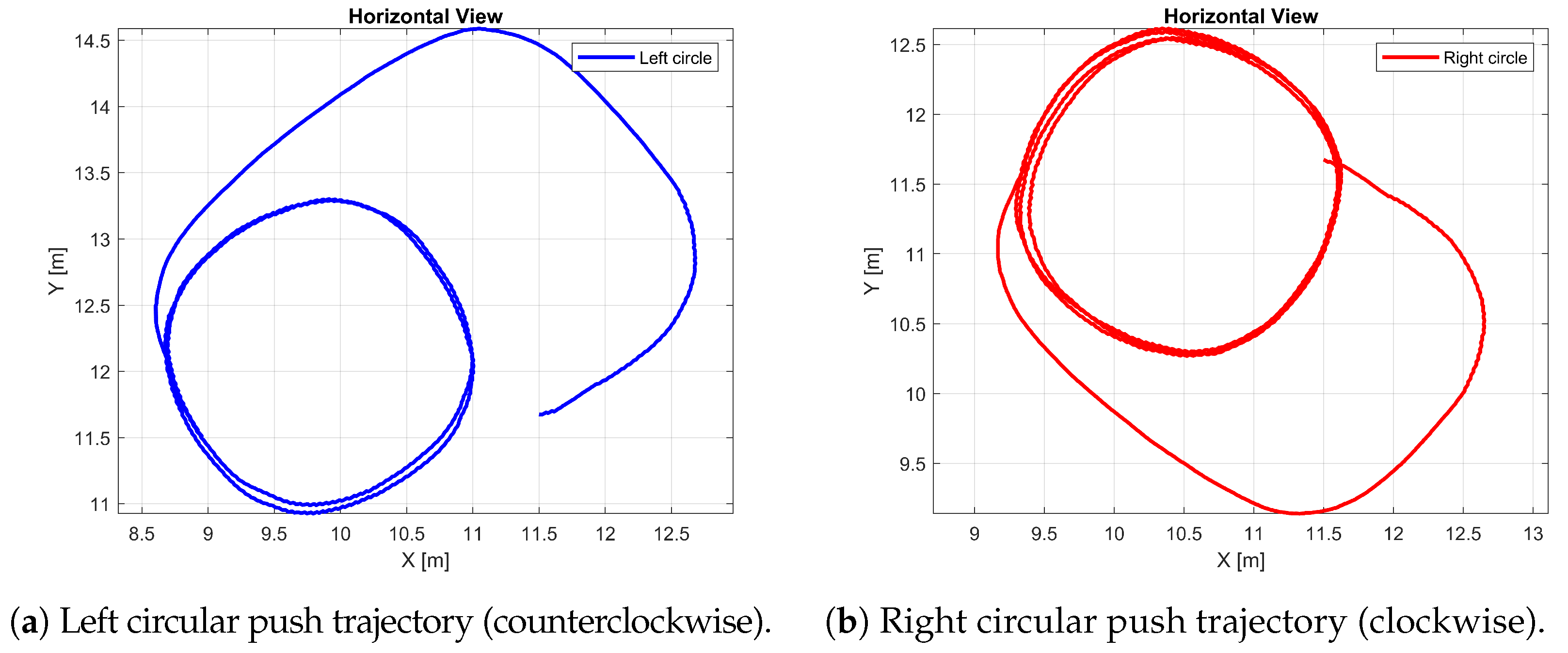
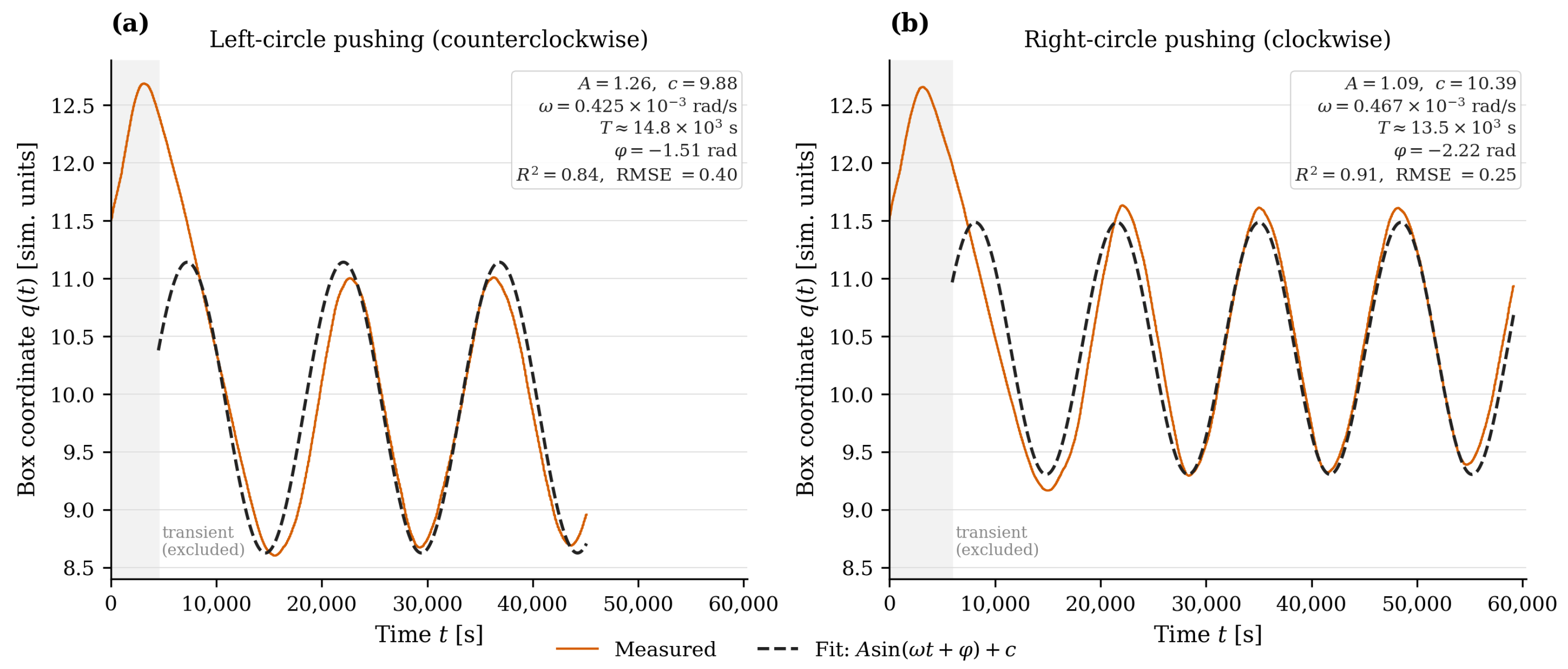
After training the agent for straight-line pushing, a deterministic extension enables circular path pushing. By applying a fixed, asymmetric Bézier action to one side, the box follows an approximately circular trajectory with a measurable rotational speed. Dubins path theory [13] shows that, for a vehicle with a minimum turning radius, planar configurations can be connected through sequences of straight segments and circular arcs. Because the box here is rotated through asymmetric pushing rather than by a steered wheel, we use the looser concept of a constant turning speed $\omega$ when composing arcs and treat the Dubins decomposition as a planning analogy whose curvature parameter is the empirically measured $\omega$ rather than a true minimum turning radius. Representative four-frame snapshots of a closed circular rollout are shown in Figure 18. Two complete left- and right-circle trajectories, recorded under identical fixed actions, are shown in Figure 19. The phase $\phi$ and rotational speed $\omega$ used for the circular motion were obtained by fitting the sinusoidal model $q\left(t\right)=A\sin (\omega t+\phi )+c$ to the recorded box coordinate signal during fixed-action pushing (Figure 20), giving:

$$\phi =\pi \left[\mathrm{rad}\right],\hspace{1em}\omega =5\times {10}^{-4} [\mathrm{rad}/\mathrm{s}]$$

(21)

Figure 18 shows the robot performing a circular pushing action in the simulation environment.

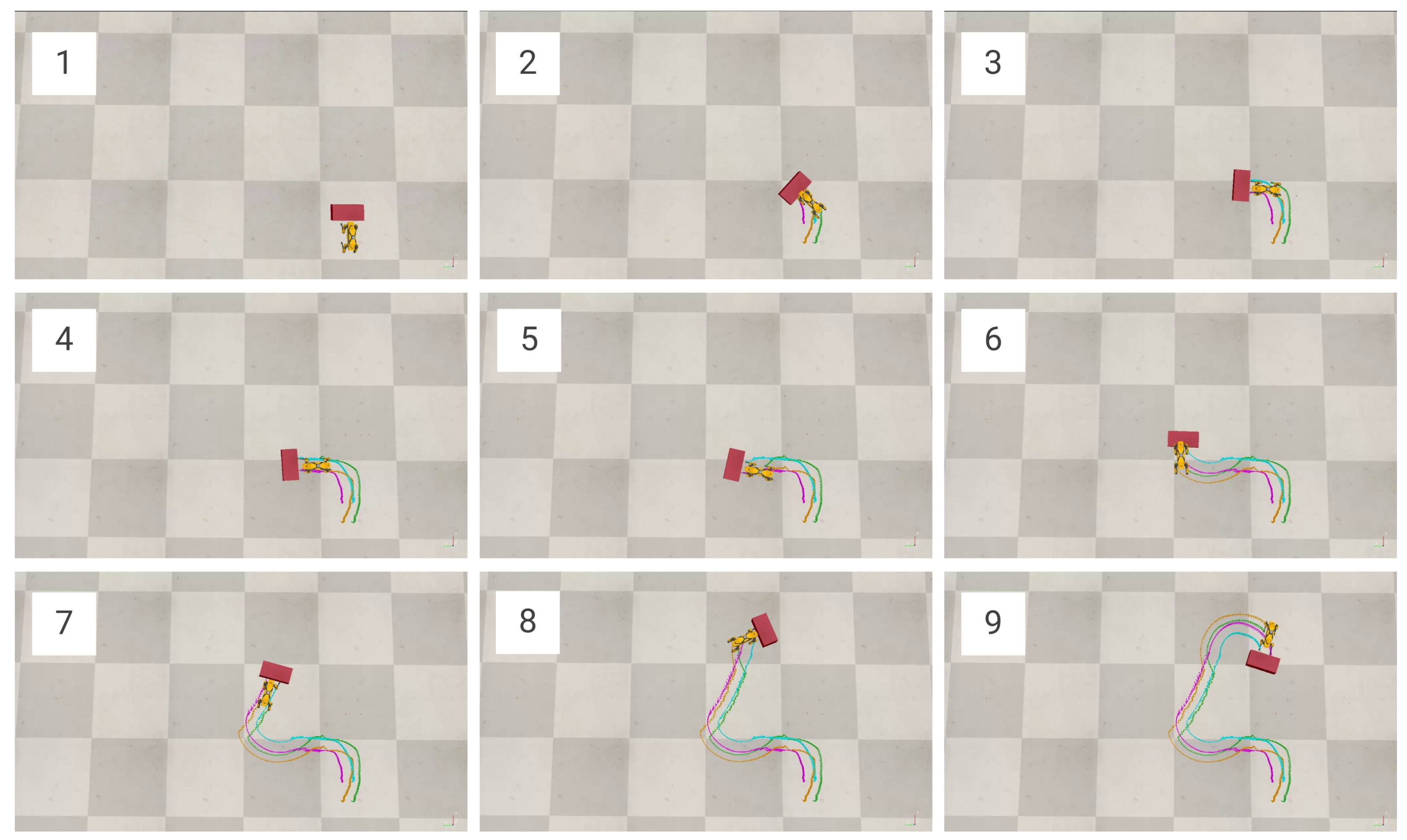
By controlling the rotational speed and direction of the circular motion, the robot can push the box along a range of curved paths composed of these arcs. Figure 20 demonstrates the ability to approximate a sine-wave reference signal by combining left and right circular arcs.

5.6. Dubins Path Extension

The combination of straight-line and circular pushing primitives connects to Dubins path theory [13], which establishes that, for a curvature-constrained vehicle, planar configurations can be connected through sequences of straight segments and circular arcs. In the original formulation, the curvature parameter is the vehicle’s minimum turning radius; in the present setting, the box is rotated by an asymmetric leg push rather than a steering input, so we substitute the empirically measured constant turning speed $\omega$ for that parameter and use this as a planning analogy for composing pushing arcs rather than as a guarantee under contact dynamics. Figure 21 illustrates this principle applied to the robot’s box-pushing task.

6. Discussion

This work demonstrates the feasibility of combining sampling-based motion planning with reinforcement learning for leg-based object manipulation by a quadruped robot. The approach builds on a long line of work on sampling-based planning [6,7,15] and policy-gradient reinforcement learning [11,36,37], and aligns with the broader trend of applying deep reinforcement learning to robotic control tasks [10,16,42,43]. Several key observations emerge from the experimental results.

Complementary strengths of RRT and PPO. The RRT algorithm [6,15] provides reliable global path planning, efficiently generating collision-free trajectories from the robot’s position to the target object; asymptotically optimal variants such as RRT* [7] and informed RRT* [8] can further refine path quality when planning time permits, while anytime RRT [14] bounds the improvement obtained between successive solutions. PPO [11], in turn, learns the fine-grained manipulation actions needed to push the box along a straight-line trajectory; the curved path behavior is produced separately by a deterministic arc-composition extension rather than being learned. This division of labor—global planning via RRT and local manipulation via PPO—mirrors the hierarchical structure of many real-world robotic tasks and is consistent with recent hybrid frameworks that combine sampling-based planners with learned controllers [24,25,26]. The same separation avoids the credit assignment difficulties that arise when a single end-to-end policy must simultaneously handle spatially extensive navigation and contact-rich manipulation [16,42].

Bézier curve parameterization. The use of Bézier curves to parameterize the leg-pushing trajectory proves effective for several reasons. First, it reduces the trajectory representation to two continuous parameters (plus leg selection and an optional push depth parameter in the variable entry configuration), keeping the action space compact and the learning problem tractable. Second, Bézier curves produce geometrically smooth leg paths, which helps reduce abrupt leg motions that could destabilize the robot, although smoothness of the geometric path does not by itself guarantee smooth joint commands or stable contact. Such smooth foot trajectories are widely used in classical legged locomotion to enforce continuous foot-tip motion and bounded acceleration [2,3,32,34], and the same arguments transfer to the pushing context here. Third, the parameterization provides intuitive control over the approach angle and contact dynamics, enabling the agent to discover diverse pushing strategies. Compared to dexterous in-hand manipulation, where high-dimensional joint trajectories must be learned directly [12,18], the present compact action space is far easier to explore and reflects the reduced contact dimensionality of leg-based pushing.

Generalization capability. The trained agent’s ability to handle box masses up to eight times the training mass suggests that the learned policy is not strongly overfit to the training mass, although confirming that it captures the underlying pushing dynamics would require evaluation across varied shapes, friction, and surface conditions. However, this is encouraging for practical applications where object properties may vary; analogous mass and dynamics robustness has been reported for learned quadruped locomotion policies [4,5] and for object manipulation policies trained with sufficiently diverse simulation distributions [12,18]. Sample-efficient off-policy algorithms, such as SAC [20,21] or DDPG [19], may further extend this generalization by allowing more aggressive randomization without exploding interaction budgets [16].

Circular path extension. The deterministic circular pushing approach, based on extracting rotational speed from fixed pushing actions, provides a simple method for extending the learned straight-line pushing to a range of curved paths. The connection to Dubins path theory [13] offers a useful analogy for composing straight and circular segments, although it does not by itself account for the contact dynamics of pushing. The Dubins decomposition has long been used in motion planning for car-like and other curvature-constrained vehicles and is naturally compatible with sampling-based planners [7,8,28] when the local steering function is replaced by the learned straight-line primitive plus arc extensions developed here.

Modular hybrid versus end-to-end design. While recent deep reinforcement learning has produced impressive end-to-end policies for complex sensorimotor tasks [12,17,18,42], jointly solving global navigation, locomotion stability, and contact-rich pushing within a single network remains data-hungry and difficult to debug [16,43]. The modular design pursued here lets each component be developed and validated independently: the gait and center-of-mass control follow established principles for statically stable walking [2,31,33,35]; the planner inherits the asymptotic properties of sampling-based methods [6,7]; and the learning component is concentrated on the narrow subspace—contact-rich pushing—where analytical models are weakest. Other hybrid planner–learner architectures with comparable motivation include RL-RRT [24], PRM-RL [25], and the RRT+PPO combination of [26], each of which reports complementary strengths from this separation of concerns.

Implications for legged manipulation. Leg-based pushing is an underexplored capability that broadens the utility of quadrupeds beyond locomotion-only deployments [4,5]. Treating a leg as an end-effector during the swing phase allows the robot to inherit its existing actuators and sensors without additional hardware, at the cost of more careful stability accounting [1,3]. The framework introduced here—global RRT planning, statically stable transitions, and a compact learned pushing primitive—is intentionally modular so that any single component can be replaced (for example, anytime [14] or informed [8] planners for navigation, off-policy continuous control algorithms [19,21] for the pushing skill, or richer footstep planners [3,34] for the underlying gait) without rederiving the whole system.

Limitations and future work. Several limitations should be noted. First, the generalization analysis only varied the box mass; different shapes, friction coefficients, ground slopes, and surface roughness remain to be evaluated, and the present results therefore characterize robustness to mass alone rather than full generalization to varied object properties. Second, the mass-robustness evaluation in Figure 16 reports one rollout per mass level: variance from random initial conditions is not captured, the linear trend lines are descriptive rather than inferential, and confidence intervals are not provided. A multi-seed extension (e.g., ten random initial conditions per mass) with error bars is the natural way to harden this analysis and is planned for the next iteration. Second, the current system operates in simulation; sim-to-real transfer would require domain randomization or other adaptation techniques and would directly benefit from recent zero-shot transfer methodologies developed for quadruped locomotion [4,5]. Third, the stability analysis relies on penalty-based enforcement rather than formal guarantees from constrained-optimization approaches [1,3]. Future work should address these limitations by extending training to diverse object properties, implementing sim-to-real transfer strategies, and developing more sophisticated stability criteria. Additionally, exploring advanced RL algorithms such as SAC [20,21], DDPG [19], or deterministic policy-gradient methods [37] could further improve learning efficiency and policy robustness, and richer reward structures grounded in the classical RL literature [9,16,36] could enable multi-object or sequential pushing tasks. Finally, the underlying simulation infrastructure—CoppeliaSim [38] together with ZeroMQ-based remote control [39] and the Stable-Baselines3 PPO implementation [40,41]—is openly reproducible and provides a natural base for these extensions.

7. Conclusions

This paper presented a hybrid framework combining the RRT algorithm with PPO-based reinforcement learning for leg-based object manipulation by a quadruped robot. The system integrates four key components: (1) a statically stable walking gait with inverse kinematics and CoM control; (2) RRT-based global motion planning with path smoothing and robot geometry adaptation; (3) PPO-based reinforcement learning with Bézier curve-parameterized leg trajectories for learning straight-line pushing; and (4) a deterministic extension for circular path pushing based on rotational speed extraction.

The experimental results demonstrate that, in the CoppeliaSim simulation, the proposed approach successfully enables a quadruped robot to navigate to a target object and push it in a straight line using the learned policy, with curved path pushing obtained through a deterministic arc-composition extension. The trained agent maintains effective pushing for box masses up to eight times the training mass; since only mass was varied, this indicates robustness to mass rather than to object shape, friction, or surface conditions. The Bézier curve parameterization of the pushing trajectory provides an effective interface between the RL agent and the physical pushing action, balancing expressiveness with learning tractability.

By assigning global navigation to a sampling-based planner and contact-rich pushing to a learned policy with a compact Bézier action space, this work shows that a quadruped can relocate objects with its legs alone—without a dedicated manipulator and without training a single end-to-end navigation-and-manipulation policy. Future work will focus on extending the methodology to diverse environments, object shapes, and real-world deployment through sim-to-real transfer techniques.

References

1. Cong, Q.; Shi, X.; Wang, J.; Xiong, Y.; Su, B.; Xu, W.; Liu, H.; Zhou, K.; Jiang, L.; Tian, W. Stability Study and Simulation of Quadruped Robots with Variable Parameters. Appl. Bionics Biomech. 2022, 2022, 9968042. [Google Scholar] [CrossRef] [Scilit] [PubMed]
2. Zhang, S.; Liu, M.; Yin, Y.; Rong, X.; Li, Y.; Hua, Z. Static Gait Planning Method for Quadruped Robot Walking on Unknown Rough Terrain. IEEE Access 2019, 7, 177651–177660. [Google Scholar] [CrossRef] [Scilit]
3. Xin, G.; Wolfslag, W.; Lin, H.C.; Tiseo, C.; Mistry, M. An Optimization-Based Locomotion Controller for Quadruped Robots Leveraging Cartesian Impedance Control. Front. Robot. AI 2020, 7, 48. [Google Scholar] [CrossRef] [Scilit] [PubMed]
4. Li, H.; Yu, W.; Zhang, T.; Wensing, P.M. Zero-Shot Retargeting of Learned Quadruped Locomotion Policies Using Hybrid Kinodynamic Model Predictive Control. In Proceedings of the 2022 IEEE/RSJ International Conference on Intelligent Robots and Systems (IROS), Kyoto, Japan, 23–27 October 2022; pp. 11971–11977. [Google Scholar] [CrossRef] [Scilit]
5. Shao, Y.; Jin, Y.; Liu, X.; He, W.; Wang, H.; Yang, W. Learning Free Gait Transition for Quadruped Robots Via Phase-Guided Controller. IEEE Robot. Autom. Lett. 2022, 7, 1230–1237. [Google Scholar] [CrossRef] [Scilit]
6. LaValle, S.M. Rapidly-Exploring Random Trees: A New Tool for Path Planning; Technical report; Computer Science Department, Iowa State University: Ames, IA, USA, 1998. [Google Scholar]
7. Karaman, S.; Frazzoli, E. Sampling-Based Algorithms for Optimal Motion Planning. Int. J. Robot. Res. 2011, 30, 846–894. [Google Scholar] [CrossRef] [Scilit]
8. Gammell, J.D.; Srinivasa, S.S.; Barfoot, T.D. Informed RRT*: Optimal Sampling-Based Path Planning Focused via Direct Sampling of an Admissible Ellipsoidal Heuristic. In Proceedings of the 2014 IEEE/RSJ International Conference on Intelligent Robots and Systems, Chicago, IL, USA, 14–18 September 2014; pp. 2997–3004. [Google Scholar] [CrossRef] [Scilit]
9. Sutton, R.S.; Barto, A.G. Reinforcement Learning: An Introduction, 2nd ed.; MIT Press: Cambridge, MA, USA, 2018. [Google Scholar]
10. Kaelbling, L.P.; Littman, M.L.; Moore, A.W. Reinforcement Learning: A Survey. J. Artif. Intell. Res. 1996, 4, 237–285. [Google Scholar] [CrossRef] [Scilit]
11. Schulman, J.; Wolski, F.; Dhariwal, P.; Radford, A.; Klimov, O. Proximal Policy Optimization Algorithms. arXiv 2017, arXiv:1707.06347. [Google Scholar]
12. OpenAI. Solving Rubik’s Cube with a Robot Hand. arXiv 2019, arXiv:1910.07113. [Google Scholar]
13. Dubins, L.E. On Curves of Minimal Length with a Constraint on Average Curvature, and with Prescribed Initial and Terminal Positions and Tangents. Am. J. Math. 1957, 79, 497–516. [Google Scholar] [CrossRef] [Scilit]
14. Ferguson, D.; Stentz, A. Anytime RRTs. In Proceedings of the 2006 IEEE/RSJ International Conference on Intelligent Robots and Systems, Beijing, China, 9–15 October 2006; pp. 5369–5375. [Google Scholar] [CrossRef] [Scilit]
15. Kuffner, J.J.; LaValle, S.M. RRT-Connect: An Efficient Approach to Single-Query Path Planning. In Proceedings of the 2000 ICRA. IEEE International Conference on Robotics and Automation, San Francisco, CA, USA, 24–28 April 2000; Volume 2, pp. 995–1001. [Google Scholar] [CrossRef] [Scilit]
16. Kober, J.; Bagnell, J.A.; Peters, J. Reinforcement Learning in Robotics: A Survey. Int. J. Robot. Res. 2013, 32, 1238–1274. [Google Scholar] [CrossRef] [Scilit]
17. Mnih, V.; Kavukcuoglu, K.; Silver, D.; Rusu, A.A.; Veness, J.; Bellemare, M.G.; Graves, A.; Riedmiller, M.; Fidjeland, A.K.; Ostrovski, G.; et al. Human-Level Control Through Deep Reinforcement Learning. Nature 2015, 518, 529–533. [Google Scholar] [CrossRef] [Scilit] [PubMed]
18. Rajeswaran, A.; Kumar, V.; Gupta, A.; Vezzani, G.; Schulman, J.; Todorov, E.; Levine, S. Learning Complex Dexterous Manipulation with Deep Reinforcement Learning and Demonstrations. In Proceedings of the Robotics: Science and Systems (RSS), Pittsburgh, PA, USA, 26–30 June 2018. [Google Scholar] [CrossRef] [Scilit]
19. Lillicrap, T.P.; Hunt, J.J.; Pritzel, A.; Heess, N.; Erez, T.; Tassa, Y.; Silver, D.; Wierstra, D. Continuous Control with Deep Reinforcement Learning. arXiv 2019, arXiv:1509.02971. [Google Scholar]
20. Haarnoja, T.; Zhou, A.; Hartikainen, K.; Tucker, G.; Ha, S.; Tan, J.; Kumar, V.; Zhu, H.; Gupta, A.; Abbeel, P.; et al. Soft Actor-Critic Algorithms and Applications. arXiv 2019, arXiv:1812.05905. [Google Scholar]
21. Haarnoja, T.; Zhou, A.; Abbeel, P.; Levine, S. Soft Actor-Critic: Off-Policy Maximum Entropy Deep Reinforcement Learning with a Stochastic Actor. arXiv 2018, arXiv:1801.01290. [Google Scholar]
22. Han, J. From PID to Active Disturbance Rejection Control. IEEE Trans. Ind. Electron. 2009, 56, 900–906. [Google Scholar] [CrossRef] [Scilit]
23. Vamvoudakis, K.G.; Lewis, F.L. Online Actor–Critic Algorithm to Solve the Continuous-Time Infinite Horizon Optimal Control Problem. Automatica 2010, 46, 878–888. [Google Scholar] [CrossRef] [Scilit]
24. Chiang, H.T.L.; Hsu, J.; Fišer, M.; Xiao, L.; Faust, A. RL-RRT: Kinodynamic Motion Planning via Learning Reachability Estimators from RL Policies. IEEE Robot. Autom. Lett. 2019, 4, 4298–4305. [Google Scholar] [CrossRef] [Scilit]
25. Faust, A.; Oslund, K.; Ramirez, O.; Francis, A.; Tapia, L.; Fiser, M.; Davidson, J. PRM-RL: Long-Range Robotic Navigation Tasks by Combining Reinforcement Learning and Sampling-Based Planning. In Proceedings of the 2018 IEEE International Conference on Robotics and Automation (ICRA), Brisbane, QLD, Australia, 21–25 May 2018; pp. 5113–5120. [Google Scholar] [CrossRef] [Scilit]
26. Chen, Y.; Ji, C.; Cai, Y.; Yan, T.; Su, B. Deep Reinforcement Learning in Autonomous Car Path Planning and Control: A Survey. arXiv 2024, arXiv:2404.00340. [Google Scholar] [CrossRef] [Scilit]
27. Zeng, A.; Song, S.; Welker, S.; Lee, J.; Rodriguez, A.; Funkhouser, T. Learning Synergies between Pushing and Grasping with Self-Supervised Deep Reinforcement Learning. In Proceedings of the 2018 IEEE/RSJ International Conference on Intelligent Robots and Systems (IROS), Madrid, Spain, 1–5 October 2018; pp. 4238–4245. [Google Scholar] [CrossRef] [Scilit]
28. LaValle, S.M.; Kuffner, J.J. Randomized Kinodynamic Planning. Int. J. Robot. Res. 2001, 20, 378–400. [Google Scholar] [CrossRef] [Scilit]
29. Lynch, K.M.; Park, F.C. Modern Robotics: Mechanics, Planning, and Control; Cambridge University Press: Cambridge, UK, 2017. [Google Scholar]
30. Craig, J.J. Introduction to Robotics: Mechanics and Control, 3rd ed.; Pearson/Prentice Hall: Upper Saddle River, NJ, USA, 2005. [Google Scholar]
31. McGhee, R.B.; Frank, A.A. On the Stability Properties of Quadruped Creeping Gaits. Math. Biosci. 1968, 3, 331–351. [Google Scholar] [CrossRef]
32. Pongas, D.; Mistry, M.; Schaal, S. A Robust Quadruped Walking Gait for Traversing Rough Terrain. In Proceedings of the 2007 IEEE International Conference on Robotics and Automation, Rome, Italy, 10–14 April 2007; pp. 1474–1479. [Google Scholar] [CrossRef] [Scilit]
33. Queiroz, C.; Gonçalves, N.; Menezes, P. A Study on Static Gaits for a Four-Leg Robot. In Proceedings of the UKACC International Conference on Control (CONTROL 2000), Cambridge, UK, 4–7 September 2000; pp. 1–6. [Google Scholar]
34. Ding, L.; Wang, G.; Gao, H.; Liu, G.; Yang, H.; Deng, Z. Footstep Planning for Hexapod Robots Based on 3D Quasi-Static Equilibrium Support Region. J. Intell. Robot. Syst. 2021, 103, 25. [Google Scholar] [CrossRef] [Scilit]
35. Kajita, S.; Kanehiro, F.; Kaneko, K.; Fujiwara, K.; Harada, K.; Yokoi, K.; Hirukawa, H. Biped Walking Pattern Generation by Using Preview Control of Zero-Moment Point. In Proceedings of the 2003 IEEE International Conference on Robotics and Automation, Taipei, Taiwan, 14–19 September 2003; Volume 2, pp. 1620–1626. [Google Scholar] [CrossRef] [Scilit]
36. Sutton, R.S.; McAllester, D.A.; Singh, S.P.; Mansour, Y. Policy Gradient Methods for Reinforcement Learning with Function Approximation. Adv. Neural Inf. Process. Syst. 2000, 12, 1057–1063. [Google Scholar]
37. Silver, D.; Lever, G.; Heess, N.; Degris, T.; Wierstra, D.; Riedmiller, M. Deterministic Policy Gradient Algorithms. In Proceedings of the 31st International Conference on Machine Learning, Beijing, China, 22–24 June 2014. [Google Scholar]
38. Rohmer, E.; Singh, S.P.N.; Freese, M. V-REP: A Versatile and Scalable Robot Simulation Framework. In Proceedings of the 2013 IEEE/RSJ International Conference on Intelligent Robots and Systems, Tokyo, Japan, 3–7 November 2013; pp. 1321–1326. [Google Scholar] [CrossRef] [Scilit]
39. Hintjens, P. ZeroMQ: Messaging for Many Applications; O’Reilly Media, Inc.: Sebastopol, CA, USA, 2013. [Google Scholar]
40. Raffin, A.; Hill, A.; Gleave, A.; Kanervisto, A.; Ernestus, M.; Dormann, N. Stable-Baselines3: Reliable Reinforcement Learning Implementations. J. Mach. Learn. Res. 2021, 22, 1–8. [Google Scholar]
41. Brockman, G.; Cheung, V.; Pettersson, L.; Schneider, J.; Schulman, J.; Tang, J.; Zaremba, W. OpenAI Gym. arXiv 2016, arXiv:1606.01540. [Google Scholar]
42. Arulkumaran, K.; Deisenroth, M.P.; Brundage, M.; Bharath, A.A. Deep Reinforcement Learning: A Brief Survey. IEEE Signal Process. Mag. 2017, 34, 26–38. [Google Scholar] [CrossRef] [Scilit]
43. Li, Y. Deep Reinforcement Learning: An Overview. arXiv 2018, arXiv:1701.07274. [Google Scholar]
Figure 1. Quadruped robot kinematic model, showing the body-frame coordinate axes ( X b , Y b , Z b ) and the segmented leg links used in the kinematic derivation.
Machines 14 00773 g001
Figure 2. Support polygon centroid. The robot shifts its CoM toward the centroid of the triangle formed by the three grounded feet ( P 1 , P 2 , P 3 ) before lifting the fourth leg for a swing phase. The filled marker, labeled COP in the figure, denotes this support polygon centroid c sp of Equation (8), i.e., the target for the horizontal CoM projection.
Machines 14 00773 g002
Figure 3. Dynamic stability during box pushing. The diagram shows the ground reaction forces at the three supporting legs and the reaction force exerted by the box on the fourth (pushing) leg, consistent with F push in Equation (9). The robot must maintain moment balance about the CoM to prevent tipping.
Machines 14 00773 g003
Figure 4. Illustration of the RRT algorithm. The tree (blue) grows incrementally from the start configuration by sampling random points and extending the nearest node, efficiently exploring the configuration space to find a feasible path (red) to the goal, which is then smoothed and adapted to the robot’s footprint (green).
Machines 14 00773 g004
Figure 5. System overview: block diagram integrating RRT-based motion planning with reinforcement learning-based manipulation. The decision block labeled Distance > 3 m keeps the robot following the RRT-planned path while it is farther than the indicated threshold from the box and switches control to reinforcement learning-based pushing once the robot is within that distance.
Machines 14 00773 g005
Figure 6. Bézier curves of increasing degree ( n = 1 to 4), shown with their control points (open circles) and control polygons (dashed lines). Additional control points increase the flexibility of the curve shape; the leg-motion parameterization used in this work is the cubic case ( n = 3 ) developed in Figure 7.
Machines 14 00773 g006
Figure 7. Schematic of the cubic Bézier leg trajectory, running from the leg’s current position P 0 to the target contact point P 3 on the box, shaped by the two intermediate control points P 1 and P 2 , which lie on a circular locus through P 0 and P 3 .
Machines 14 00773 g007
Figure 8. Family of candidate Bézier leg-swing trajectories in 3D (leg-tip coordinates), spanning the range of paths from the rest position toward the contact point on the box. The colors serve only to distinguish the individual candidate trajectories and carry no additional meaning.
Machines 14 00773 g008
Figure 9. Representative leg-on-box pushing sequence (panels (1)–(6), in chronological order, (top-left) to (bottom-right)): close-up of a single Bézier-parameterized leg swing contacting and pushing the box face in CoppeliaSim. The six panels span the last three seconds of the leg-swing Supplementary Video S4; across the panels, the pushing leg descends along its Bézier trajectory (Equation (14)), makes contact with the upper-right edge of the box, and applies a lateral push, which contributes to the box-pose change penalized by Equation (16).
Machines 14 00773 g009
Figure 10. System architecture for the RRT-based motion-planning and simulation-execution pipeline. MATLAB plans and smooths the path, Python bridges the planner to the simulator, and CoppeliaSim executes the leg motion. Solid arrows mark the forward command flow; dashed arrows mark the feedback/state-update flow. The reinforcement learning training loop is shown separately in Figure 11.
Machines 14 00773 g010
Figure 11. Reinforcement learning loop between the PPO agent and the CoppeliaSim environment. At each step, the agent sends the action a t = [ w 1 , w 2 , leg   ID ] (Bézier control parameters and the selected pushing leg) to the simulator. CoppeliaSim executes the motion, updates the robot–box state, and returns the next observation s t + 1 , the scalar reward R t , and a step-completion flag. The reward is computed after execution from the box–target position error, angular error, and a fall penalty (Equation (16)).
Machines 14 00773 g011
Figure 12. Actor–critic network architecture. Both networks consist of four hidden layers with 512 neurons and ReLU activations. The actor outputs action means; the critic outputs the state value.
Machines 14 00773 g012
Figure 13. Qualitative comparison of RRT motion planning and execution. (a) MATLAB planning view in the world frame: black = obstacles, blue = RRT tree, red = raw planned path, and green = smoothed footprint-adapted path (axes in meters). (b) Perspective screenshot of the robot in CoppeliaSim executing the same plan; the colored curves are the four leg-tip traces accumulated during execution. The two views share only the start orientation and are not registered in a common coordinate frame.
Machines 14 00773 g013
Figure 14. Moving average (window size = 30) of the cumulative reward per episode with its confidence interval for the fixed entry value configuration. The sharp increase over the first 50 episodes, followed by a plateau, indicates that learning has largely saturated.
Machines 14 00773 g014
Figure 15. Moving average (window size = 30) of the cumulative reward per episode with its confidence interval for the variable entry value configuration. The cumulative reward increases over training, with the rate of improvement decreasing toward the end of the run, despite the larger action space dimensionality; the confidence interval remains comparatively wide.
Machines 14 00773 g015
Figure 16. Mass-robustness evaluation of the trained pushing agent: both errors increase approximately linearly over the tested range, with no abrupt divergence observed. Eight box mass levels were tested, with one evaluation at each. The horizontal axis is the relative mass increase Δ m / m train , where m train = 0.1 kg; Δ m / m train = 800 % corresponds to adding 0.8 kg, for a total box mass of 0.9 kg. Filled circles are observations; the dashed gray line is a descriptive linear trend (intercept constrained to be non-negative). (a) Angular error grows from 0.59 ° at Δ m / m train = 0 to 6.32 ° at Δ m / m train = 800 % . (b) Position error grows from 0.18 m to 0.64 m. With n = 8 single-run observations per panel, the fits are descriptive guides rather than inferential models.
Machines 14 00773 g016
Figure 17. Straight-line pushing result. (a) Eight chronological overall-view frames from a representative straight-line rollout (Video S2), each zoomed to keep the robot centered via yellow-chassis tracking and stamped with the rollout timestamp. (b) Eight chronological close-up frames from the Supplementary Video S6 showing one leg pushing the box, with the leg-tip Bézier curve trajectory rendered in green on the CoppeliaSim view. (c) Recorded XY trajectories of the two tracked box corners with corresponding target markers. The corners advance toward the targets along an approximately straight but visibly stepwise path. Axes are in meters.
Machines 14 00773 g017
Figure 18. Box pushing along a circular path in the CoppeliaSim simulation environment: four snapshots from a single deterministic rollout (Section 5.6) showing how the leg-tip traces (colored arcs) accumulate as the robot drives the box around a full loop. (a) Initial pose, with the quadruped beside the box and no trace yet visible. (b) After approximately 9 s, a partial arc has been traced as the robot completes the first quarter of the circle. (c) After approximately 17 s, more than half of the circle has been traced. (d) After approximately 25 s, a complete circular trajectory has been closed; the multiple overlapping colored rings correspond to the trajectories of the four leg tips during the swing-and-push cycle. Timestamps are wall-clock times from the recorded video.
Machines 14 00773 g018
Figure 19. Approximately circular box-pushing trajectories. (a) Left (counterclockwise) and (b) right (clockwise) arcs achieved using deterministic fixed actions. Each trace includes transient segments and some irregular looping at the start and end of the motion before settling into an approximately circular arc. By controlling the rotational speed and direction, a range of arc-based paths can be constructed.
Machines 14 00773 g019
Figure 20. Tracked box coordinate under deterministic circular pushing follows an approximately sinusoidal trajectory in both rotation directions, supporting the use of a sinusoidal model to parameterize the arc-based motion. (a) Left-circle (counterclockwise) and (b) right-circle (clockwise) pushing: the solid line is the measured box coordinate q ( t ) recorded during a fixed-action rollout; the dashed line is the fitted model q ( t ) = A sin ( ω t + φ ) + c , refitted independently per panel. The fit is performed on the steady-state segment after an initial transient (shaded region, excluded); the per-panel values of A, ω , T = 2 π / ω , φ , c, together with the coefficient of determination R 2 and root-mean-square error, are annotated. The recovered rotational speed is ω 4 5 × 10 4 rad/s in both panels and is consistent with the deterministic value used in Equation (21); the per-panel phase reflects the direction-dependent initial condition of each rollout. The vertical axis is in CoppeliaSim simulation units (the recorded coordinate is one component of the box centroid relative to the simulation origin).
Machines 14 00773 g020
Figure 21. Frame sequence (19) illustrating a Dubins-style box-pushing path, in which the box is driven from a start toward a goal configuration using a combination of straight pushes and circular arcs. The individual straight and circular segments are not separately annotated in the frames.
Machines 14 00773 g021