FMEA-Guided Selective Multi-Fidelity Modeling for Computationally Efficient Digital Twin-Based Fault Detection

Abstract

Autonomous navigation technologies have been widely adopted in the automotive and aviation sectors, significantly reducing human-error-induced accidents and operational costs. However, their application to maritime systems remains limited due to the complexity of conventional propulsion systems. Electric propulsion ships, with well-defined system boundaries and accessible operational data, offer a promising platform for autonomous navigation. In this study, we propose an FMEA-guided selective multi-fidelity digital twin framework for fault detection, where model fidelity is adaptively selected between low- and high-fidelity models based on risk priority numbers derived from failure mode and effects analysis. This approach enables selective execution of computationally expensive models only under high-risk conditions, thereby improving computational efficiency. In addition, a sliding window-based algebraic aggregation method is employed to achieve lightweight and real-time fault diagnosis. The proposed framework is validated using operational sensor data from a 100 kW electric propulsion ship under multiple fault scenarios, including power supply faults and signal anomalies. Experimental results show that the proposed method reduces computational cost while maintaining stable real-time performance, compared to conventional data-driven AI-based approaches. These results demonstrate that the proposed framework provides an effective and efficient solution for enhancing the reliability and safety of autonomous ship systems.

1. Introduction

1.1. Background

Autonomous operation technologies are rapidly gaining prominence across the mobility sector, particularly in aviation and automotive domains. This trend can be attributed to the several advantages offered by autonomous systems in terms of operational efficiency. For example, in the aviation sector, drone delivery reduces dependence on human labor, thereby lowering personnel costs [1]. In the automotive sector, robotaxis can reduce energy consumption by analyzing real-time data on traffic conditions, weather, and energy usage. Moreover, robotaxis facilitate in minimizing human errors that occur during manual operation [2,3]. These examples illustrate technologies that have already reached advanced stages of development and are progressing toward commercialization.

To align with these developments, the maritime mobility sector is placing increasing emphasis on autonomous operations for ships. Human error accounts for approximately 85% of recurring maritime accidents, and issues, such as the aging of seafarers, have further intensified the need to develop autonomous ships [4]. However, most propulsion systems in currently operating vessels are based on internal combustion engines, which present several challenges in the implementation of autonomous navigation. Internal combustion engines involve complex interactions between multiple physical phenomena, including combustion, heat transfer, and friction, which result in highly intricate system dynamics and ambiguous system boundaries. This characteristic is inherently incompatible with the high-precision model-based predictive control required for autonomous navigation technologies [5,6,7,8]. By contrast, electric propulsion ships feature a relatively simple and clearly defined structure, comprising a power generation source, switchboards, a power converter, and an electric motor. In addition, key operational data, such as the current, voltage, frequency, and state of charge (SOC), can be quantitatively measured. These data exhibit linear or weakly nonlinear characteristics, thereby facilitating system modeling and predictive control [9,10]. Accordingly, the adoption of electric propulsion is indispensable for the practical realization of autonomous ship operations.

Autonomous navigation of ships can be categorized into four levels: Levels 1 and 2 correspond to manned vessels that require crew members to be onboard, whereas Level 3 enables remote control of the vessel from the shore. The final stage, Level 4, represents fully unmanned autonomous ships, which constitutes the ultimate objective of autonomy in maritime mobility [11]. However, unlike land-based systems, ships operate in isolated maritime environments where immediate external assistance is unavailable in the event of an accident. Consequently, delays in the initial response may lead to a rapid escalation of damage, resulting in significant damage to both property and the environment. Therefore, autonomous ship systems must incorporate fault detection and management frameworks capable of promptly identifying system failures and executing optimized response procedures [12,13,14,15]. Furthermore, under actual maritime operating conditions, failures can vary widely in terms of their type, severity, and frequency. Uniform responses to all types of failures can result in inefficient resource allocation and potentially prevent adequate responses to high-risk failures. Therefore, ensuring the safety of autonomous ships requires appropriate fault diagnosis and management strategies.

Despite these requirements, existing maritime research has limitations. Digital twin approaches have primarily focused on one-dimensional data visualization, while fault diagnosis methods often rely on either single high-fidelity models or computationally expensive artificial intelligence techniques. These limitations hinder the development of efficient and scalable real-time diagnostic systems for autonomous ships operating under diverse failure conditions.

Contributions of this study are summarized as follows:

• Risk-based fidelity optimization framework:

This study proposes a novel framework that determines model fidelity using Risk Priority Number (RPN) values derived from FMEA. High-risk failures are analyzed using high-fidelity models (HFMs) for accuracy, whereas low-risk failures are handled using low-fidelity models (LFMs) for computational efficiency. This risk-driven fidelity selection approach has not been previously explored in maritime digital twin research.

2.

Lightweight real-time fault diagnosis method:

Instead of relying on computationally expensive artificial intelligence techniques, this study introduces a sliding window algebraic aggregation method to reduce computational overhead and enable real-time fault diagnosis. This design is particularly suitable for operational environments such as autonomous ships.

3.

Integration with real-world data and system validation:

A data pipeline was developed using real-world data collected from an electric propulsion ship and integrated with a remote-controlled user interface. The proposed framework was validated using actual operational data, demonstrating its practical applicability.

4.

Practical guidelines through propulsion system case study:

A case study on propulsion motor failure scenarios provides concrete guidelines for diagnostic delay times and threshold setting, demonstrating that the proposed framework is deployable in real-world systems.

5.

Enhancement of safety in autonomous ship operations:

The proposed approach addresses critical risks associated with single-line propulsion configurations, where failures may lead to total propulsion loss. By combining risk-based fidelity selection with lightweight diagnostic structures, the framework improves the safety and reliability of autonomous ships.

1.2. Literature Review

The most reliable approach for the fault diagnosis of a system is to compare the current system state with its nominal condition. To achieve this, a nominal model that accurately replicates the physical behavior of an actual system is required. In this context, digital twin technology has recently emerged as a promising solution. A digital twin is defined as the digital replica of a physical system [16]. This technology is primarily employed for real-time monitoring, predictive maintenance, fault detection and diagnosis, and the optimization of operational processes, thereby providing significant support for system operations [17,18,19]. However, in the maritime domain, digital twin applications have predominantly been limited to external or structural representations of ships. Hence, as in other fields, there is a growing need for digital twin research that integrates the internal systems of ships.

A critical consideration in digital twin modeling is fidelity, which refers to the accuracy and complexity of a model and indicates the extent to which it can replicate an actual system. Although ideal modeling would reproduce a real system with complete accuracy, computational resources are inherently limited. Therefore, maintaining a balance between model accuracy and computational cost is essential. Digital twin frameworks typically employ high-fidelity models (HFMs) and low-fidelity models (LFMs). HFMs provide detailed simulations of the behavior of a physical system. However, they are computationally expensive and require long simulation times, making them unsuitable for real-time applications. By contrast, LFMs simplify specific details relative to HFMs, resulting in a lower accuracy but significantly reduced computational costs and faster simulations, rendering them more suitable for real-time applications. Given these characteristics, the fidelity of a digital twin model must be selected based on the specific purpose of the simulation [20,21,22].

Applying the same fidelity level across the system is suboptimal: HFMs will be impractical for real-time applications owing to their computational burden, whereas LFMs will suffer from reduced accuracy. Therefore, to establish objective criteria for selecting the fidelity level of a digital twin model, a systematic fault analysis step is required. This step enables the selection of fidelity levels based on the severity of potential failures, thereby optimizing computational resource usage. The fault tree analysis (FTA) is a technique that traces the underlying causes of system failures. Unlike a simple enumeration of failure modes, the FTA enables logical analysis of failure propagation. However, it primarily yields qualitative results, making it challenging to prioritize failures based on their likelihood of occurrence or severity [23,24]. Consequently, high-criticality failures may not receive timely attention, which is particularly hazardous for ships that do not feature immediate external support.

The hazard and operability study (HAZOP) method is an additional qualitative approach primarily used to identify potential failure scenarios within process flows and devise preventive measures. HAZOP is suitable for the systematic examination of abnormal states and preventive action planning [25]. However, because its analysis is generally performed at the process-line level [26,27,28], direct integration with ship operations is challenging, as operational data in ships are typically collected at the component level.

By contrast, the failure mode and effects analysis (FMEA) can identify potential component or system-level failures in advance, evaluate their impact on overall system performance, and quantitatively assess risk [29,30,31]. The primary objective of the FMEA is to prioritize high-risk failure modes for improvement. It is particularly suitable for autonomous ships, where the early identification of failures and prioritization of countermeasures are essential. The FMEA has been widely applied not only in safety-critical industries, such as the aviation, automotive, maritime, and defense industries, but also across the manufacturing, maintenance, and quality management domains [32,33,34]. More recently, the FMEA has been integrated with digital twin and predictive maintenance systems, extending its application to real-time fault diagnosis and countermeasure planning [35,36].

The selection of an appropriate fault diagnosis method is crucial for detecting failures between digital twin models and actual ship operations employing data analysis. Among the various fault diagnosis techniques, the adaptive window approach dynamically adjusts the window size based on data variation, thereby enabling the sensitive detection of abnormal segments. However, because the window length is not fixed, this approach has limited compatibility with digital twin models, necessitating additional data postprocessing steps such as padding or masking [37,38,39]. Consequently, this method is unsuitable for applications in ship-based digital twin systems, where real-time performance is critical. By contrast, the sliding-window method partitions data into fixed-length segments, thereby enabling fault diagnosis with consistent input sizes. This property ensures high compatibility with digital twin models, eliminating the need for postprocessing. Moreover, the sliding-window method is robust when applied to real-time data subjected to communication delays or noise [40,41,42]. Therefore, this study adopted the sliding-window method owing to its superior performance in terms of real-time applicability, model compatibility, and stability.

Table 1. Summary of prior research.

Ref.	Approach/Method	Limitations	Fidelity
[43]	Data-driven digital twin using machine learning	High computational demand, lack of physical interpretability	Data-driven (not explicitly defined)
[44]	High-fidelity multi-physics EV digital twin	High model complexity and computational burden	High (fixed)
[45]	DT-based fault diagnosis using simulated data + domain adversarial graph neural network	High modeling complexity; domain gap between simulated and real data	High (physics-based, fixed)
[46]	DT-based composite fault diagnosis using virtual and real data	System-specific modeling; fidelity and computational cost not explicitly analyzed	Not explicitly defined
[47]	DT-based gearbox fault diagnosis using physical–virtual data fusion	Requires high-fidelity modeling and still depends on limited real fault data; virtual–physical data gap exists	High (physics-based, validated)
[48]	DT-assisted fault diagnosis using virtual data only with VMD-based feature extraction	Difficulty in high-fidelity modeling; virtual–physical data gap; limited fault generalization	High (physics-based, fixed)
[49]	DT-based data augmentation for imbalanced fault diagnosis using MDOF model and FBC-GAN	Simulation–real data gap; dependence on GAN mapping; need for real data; limited data diversity	High (physics-based + data-driven hybrid)
[50]	DT-driven partial domain fault diagnosis using adversarial transfer learning with weighting module	Virtual–physical distribution gap; assumption on fault type coverage; sensitivity to noise; limited accuracy	Moderate–High (validated but imperfect)
[51]	DT-based aero-engine fault diagnosis using deep multimodal fusion (DBM + MFNN) with degradation adaptive correction (DAC)	Model mismatch; nonlinear system limitation; noise sensitivity; difficulty in PBM–DDM fusion	Moderate–High fidelity (validated with real engine, but mismatch exists)
[52]	DT-driven diesel engine fault diagnosis using RF classification and optimization–simulation coupled virtual model	High database construction cost; system complexity; dependence on virtual model accuracy; use of simulated fault data	Moderate (validated physics-based model)

presents a summary of prior research on digital twins, model fidelity, and fault diagnosis methods.

2. Proposed Method

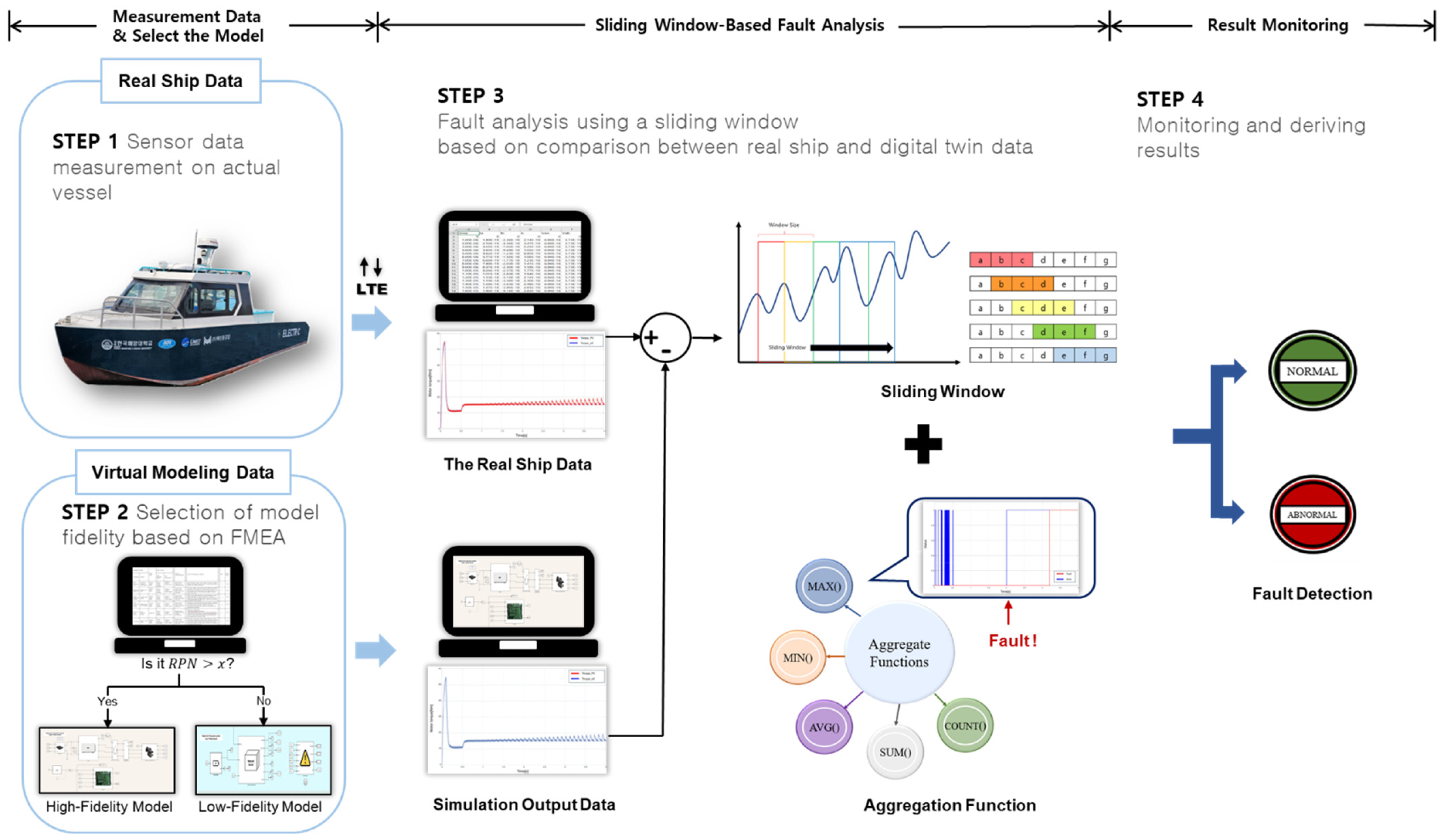
This study proposes a digital twin-based real-time fault diagnosis method for electric propulsion ships that incorporates fidelity models selected based on the results of the FMEA. The proposed method involves the following four steps:

Step 1: Operational data from an actual electric propulsion ship are transmitted in real time to a shore-based control center.

Step 2: A digital twin ship modeled in a MATLAB/Simulink (ver. 2025a) environment with the same configuration as a real vessel helps simulate the nominal operating state. To accurately reproduce the physical behavior, the digital twin model includes detailed implementations of key components such as the battery system, inverter, and propulsion motor. In this stage, fidelity levels are determined based on RPN values derived from the FMEA, considering both computational resources and real-time applicability. High-risk components are simulated using HFMs to capture the detailed dynamics, whereas low-risk components are modeled using simplified low-fidelity representations to enhance operational efficiency.

Step 3: The nominal states generated by the digital twin are compared with real ship data for fault diagnosis. For this purpose, we employed the sliding-window technique, which partitions continuous data into smaller segments, making it highly suitable for comparative analysis. Aggregation functions, such as MIN, MAX, and COUNT, are then applied to determine whether thresholds are exceeded or to measure the frequency of exceedances, thereby enabling fault detection.

Step 4: Finally, the system enables real-time monitoring of the fault occurrence.

Figure 1 shows an overview of the proposed framework, which combines fidelity selection based on the FMEA with a digital twin for real-time fault diagnosis.

2.1. STEP 1—Measuring and Transmitting Ship Data

Table 2. Specifications of the 100 kW electric propulsion ship.

Item	Specification
Owner	Korea Maritime & Ocean University, Marine Application Substantiation Technology Center (MASTC)
Vessel type	Test vessel
Length/beam	8.0 m/2.5 m
Power output	100 kW
Power source	80 kW (Li-ion battery pack)
Main engine	Permanent magnet synchronous motor (PMSM) 1 set
Inverter	120 kW × 1 unit
Propulsion motor	150 kW (peak) × 1 unit

presents the basic specifications of the 100 kW electric propulsion system employed in this study.

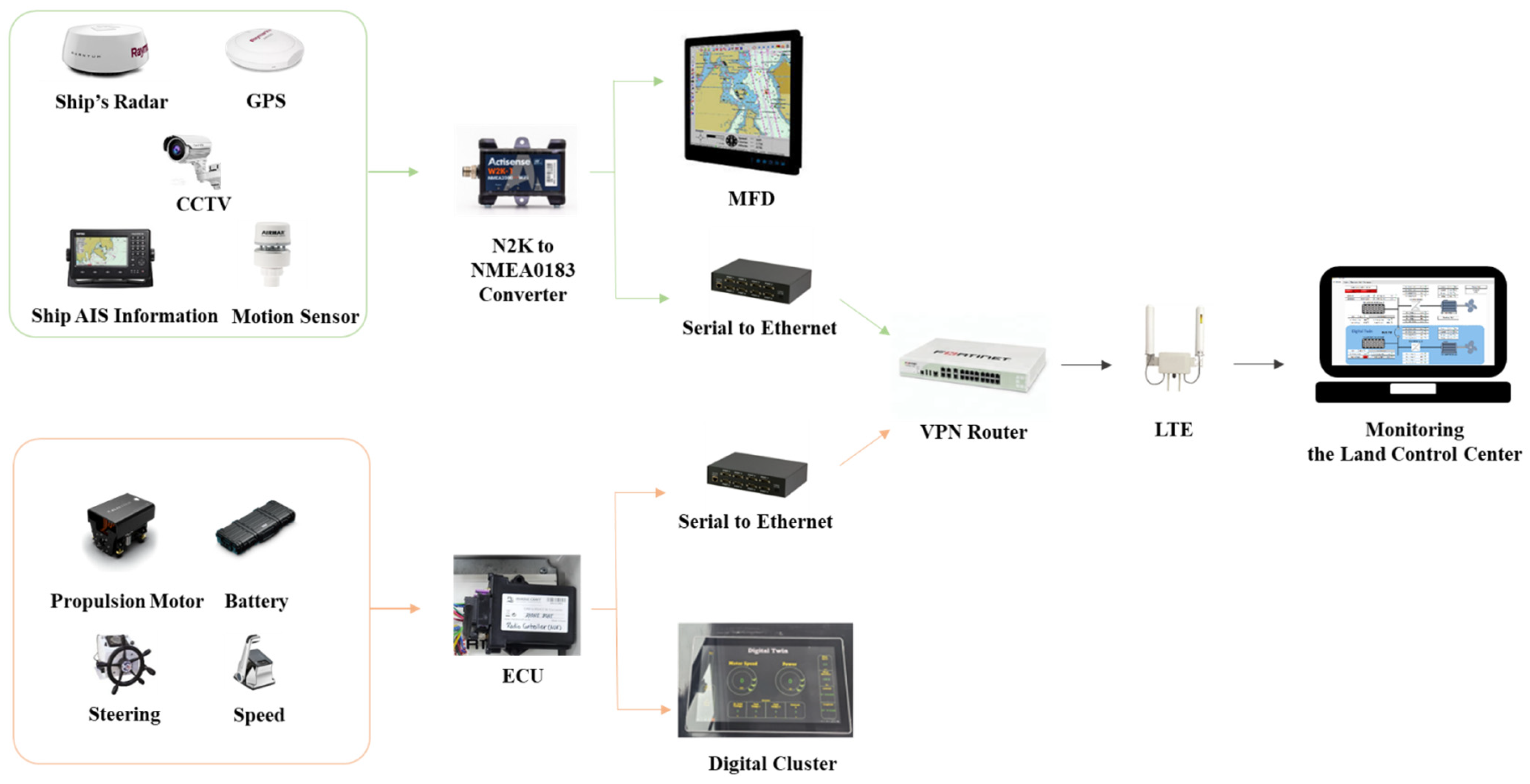
The navigational equipment installed on the ship (e.g., radar, GPS) generated data in the form of NMEA 2000 or NMEA 0183 signals, which were input into the central hub. These data were then displayed onboard on a multifunction display (MFD) console. In addition, the same signals were converted into Ethernet format via a serial-to-Ethernet converter and subsequently stored on an onboard server computer through LAN connections. Data from the electric propulsion system, including the battery, inverter, and propulsion motor, were transmitted via CAN 2.0b communication and displayed on an onboard digital cluster monitor. In particular, the battery, which served as the ship’s power source, provided real-time information, such as the current, SOC, and individual cell voltages, through the cluster monitor.

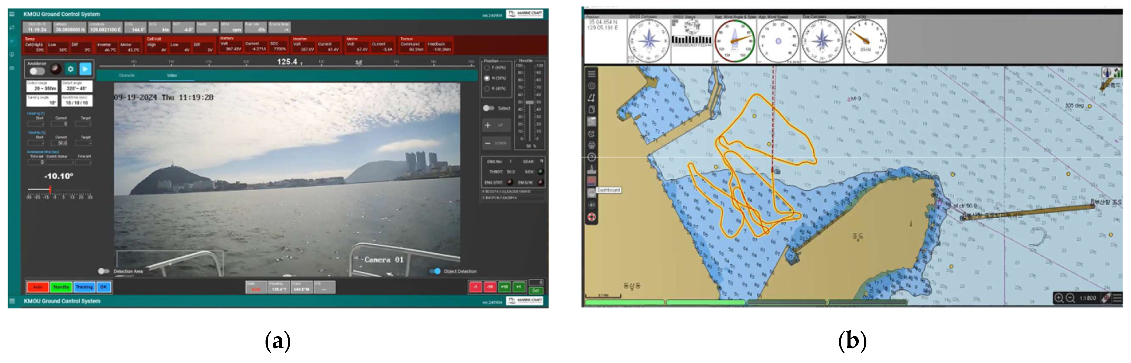
All the measured data were collected using a dedicated data acquisition unit. This unit receives current and voltage signals from various measurement devices and converts them into analyzable data formats. The converted data were stored on an onboard PC using Ethernet. Subsequently, the collected operational data were transmitted to the shore-based control center through an LTE-based data link operating in an encrypted one-to-one VPN environment. The transmitted data were automatically logged on the server at intervals of 0.1 s. At the shore-based control center, a LabVIEW-based data acquisition system was deployed, enabling real-time monitoring of the ship’s operating status. Figure 2 illustrates the real-time monitoring of the actual ship operation at the shore-based control center.

The following procedure must be performed to enable shore-based monitoring. First, the NMEA 0183 signals received from the ship were parsed and converted into a format identical to that displayed on the onboard MFD console. This conversion allowed the operating status of the vessel to be accurately monitored, as if observed directly from within the ship. For real-time data transmission and reception, a network stream protocol implemented in the LabVIEW-based program was utilized. The network stream method operates on a unidirectional communication structure, establishing a fixed one-to-one communication channel between the sender and the receiver. This feature ensured rapid data transfer and reliable communication without data loss. Moreover, LabVIEW provided built-in network stream functions and related properties, which simplified system implementation [53,54]. Based on this approach, the data acquisition systems of both the actual ship and shore-based control center were constructed using LabVIEW. Specifically, the input and output of the NMEA 0183 signals were managed using LabVIEW on the server and supervisory computers. Figure 3 illustrates the conversion and transmission flows of the measured data.

2.2. STEP 2—Determining the Fidelity of the Digital Twin Model Using FMEA

The computation time of a digital twin is directly influenced by the accuracy and complexity of the model, with higher accuracy inevitably leading to greater complexity. As a result, the digital twin model may exhibit slower response times than the actual system, causing time-delay issues. However, for real-time fault detection, the time difference between the digital twin and real system must be minimized. This necessitates careful consideration of model fidelity, which reflects both the accuracy and complexity of the model.

Fidelity is an indicator of how precisely and in detail a model reproduces the behavior of an actual system. HFMs provide detailed representations of the target physical system, capturing effects such as inverter switching harmonics. Although this enables highly accurate simulation results, it also significantly increases computational costs and may lead to time delays. By contrast, LFMs simplify the physical behavior by omitting specific details, thereby reducing the simulation time requirements. However, this simplification inherently reduces the accuracy compared with HFMs. Therefore, the selection of an appropriate fidelity level must consider simulation objectives, hardware specifications, and operational environment, particularly when real-time applications are required. In this study, a low-fidelity inverter model was developed by simplifying its representation relative to its high-fidelity counterparts. Specifically, an average model that approximates the behavior of the inverter over the switching periods was adopted. This approach effectively reduces the computational burden while still capturing the essential dynamics of inverter operation, thereby achieving a balance between accuracy and efficiency.

To selectively employ models with different fidelity levels depending on operational conditions, an objective selection criterion is required. The FMEA was adopted to establish this criterion. Originally developed by the U.S. Department of Defense as a risk assessment methodology to evaluate system reliability, the FMEA has been widely applied not only in safety-critical industries, such as aerospace, automotive, maritime, and defense, but also across the manufacturing, maintenance, and quality management domains [32,33,34]. More recently, the FMEA has been integrated with digital twin and predictive maintenance systems, enabling real-time fault diagnosis and the formulation of response strategies [35,36]. The FMEA can be classified into three categories: design FMEA, process FMEA, and equipment FMEA. For ship applications, the equipment FMEA is the most appropriate because it focuses on analyzing the operational states of the vessel [55,56]. This method systematically evaluates potential failures, their causes, consequences, and associated risks for each system component [29,30,31].

The procedure of the FMEA is as follows. First, potential failures at the system or component level were identified, and their effects on the overall system were analyzed. Subsequently, each failure mode was quantitatively assessed in terms of the risk. Three criteria were used for the evaluation: severity (S), which measures the seriousness of the effect of failure; occurrence (O), which indicates the likelihood of failure occurrence; and detection (D), which assesses the ability to detect failure in advance. Each criterion was rated on a scale of 1 to 10, and its product yielded the RPN, which numerically represented the risk level. A higher RPN indicates a higher priority for corrective action in the corresponding failure mode [57,58].

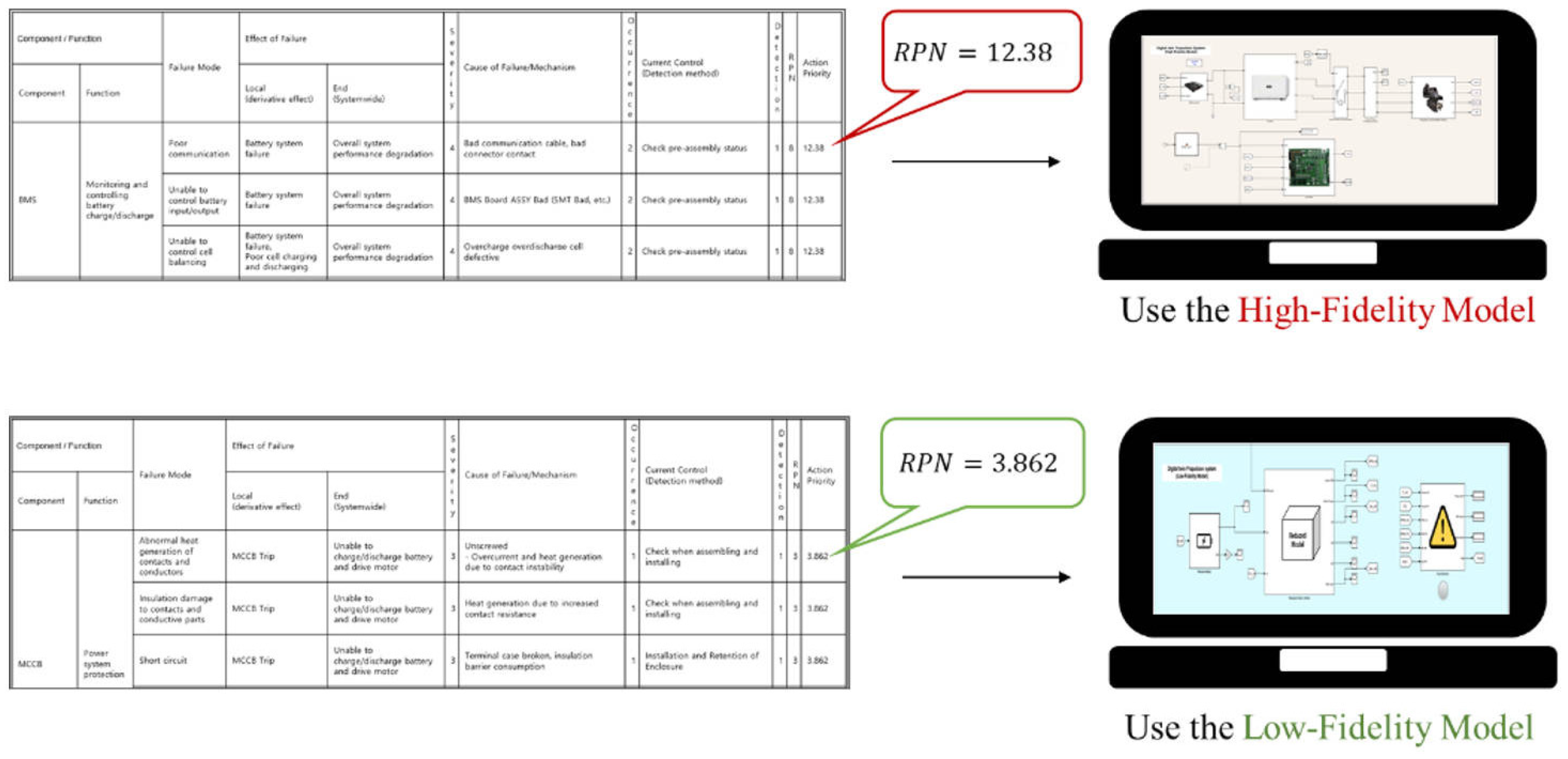
In this study, the FMEA was conducted to determine the appropriate fidelity levels of the models. The propulsion system was first decomposed into its constituent components, and the specific functions performed by each component within the overall system were defined. The potential failure modes were then enumerated for each component. For every identified failure mode, its impact at the component level, as well as on the overall system, was analyzed, and the underlying causes were systematically investigated. Based on these analyses, severity, occurrence, and detection were evaluated, and the RPN was subsequently calculated. Typically, when the RPN is calculated as a simple arithmetic product, equal weights are assigned to severity, occurrence, and detection [59]. However, in this study, each factor had a different level of importance. To address this limitation, we computed a weighted RPN that incorporated the relative significance of each factor. Based on this, classification criteria for the weighted RPN were established, and models with different fidelity levels were selectively employed on the basis of these criteria. Specifically, values from 1 to 5 were considered low risk, values from 5 to 15 as moderate risk, and values greater than 15 as high risk. Considering that ships are inherently vulnerable to failures owing to their operational characteristics, the HFM was applied for the moderate-risk category and above. Figure 4 illustrates the overall process of the fidelity model selection based on the RPN. The specific data are provided in Appendix A.

The digital twin model of the electric propulsion ship was developed in MATLAB/Simulink regardless of the fidelity level. For instance, when modeling an inverter, the key difference between HFMs and LFMs lies in whether inverter switching is explicitly simulated to reproduce the actual output waveform (HFM) or whether an averaged model is employed to compute the output values (LFM). In an actual ship, the inverter operates at a switching frequency of 12 kHz; therefore, in the HFM, both the simulation step size and sampling period must be extremely small. This requirement significantly increases computational demands, necessitating the use of high-performance CPU/GPU resources.

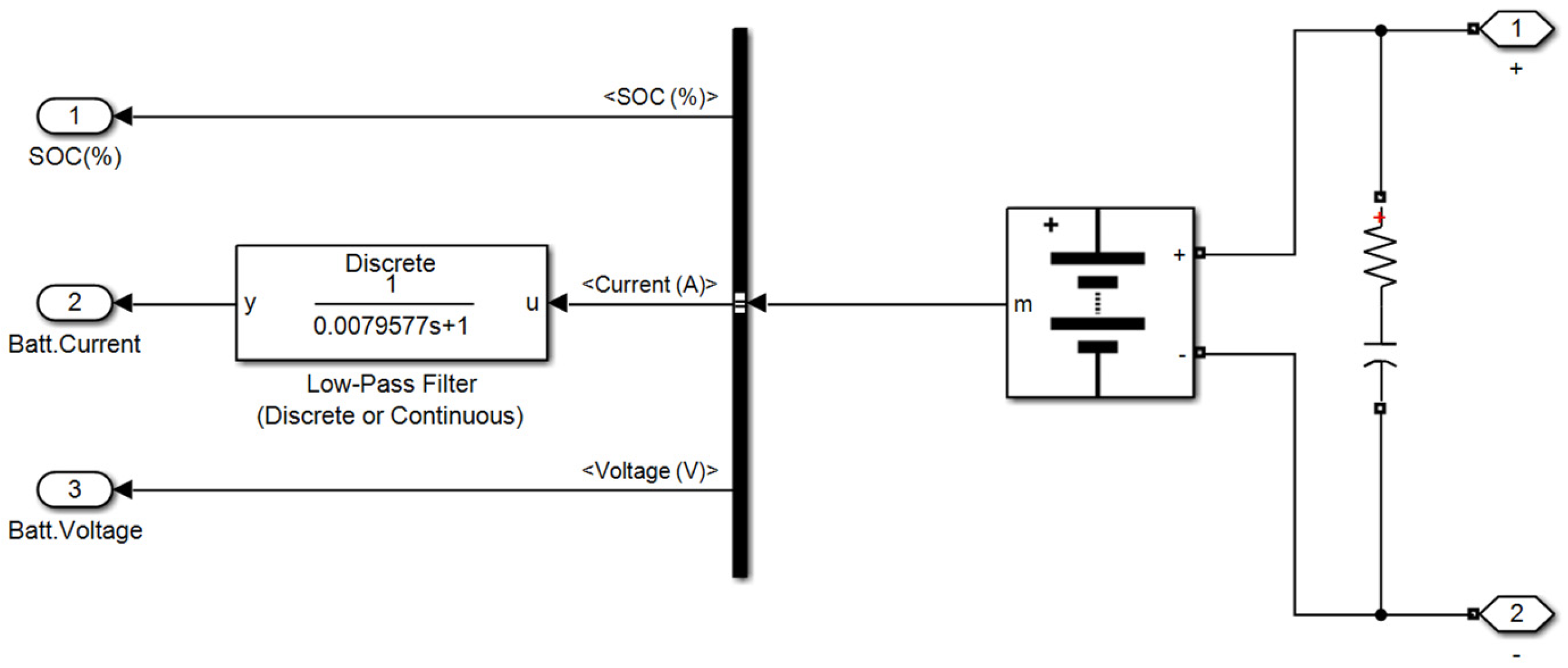
For the battery system, a library-based battery block was employed to construct a baseline model using the battery parameters of an actual ship. To capture the dynamic characteristics, additional resistance and capacitance were connected to the output of the battery block. The system was then modularized into a subsystem by incorporating an outport and a connection port. Moreover, to suppress the noise arising from power semiconductor switching, a low-pass filter was added to the current measurement port. Figure 5 illustrates the battery system used in the digital twin model.

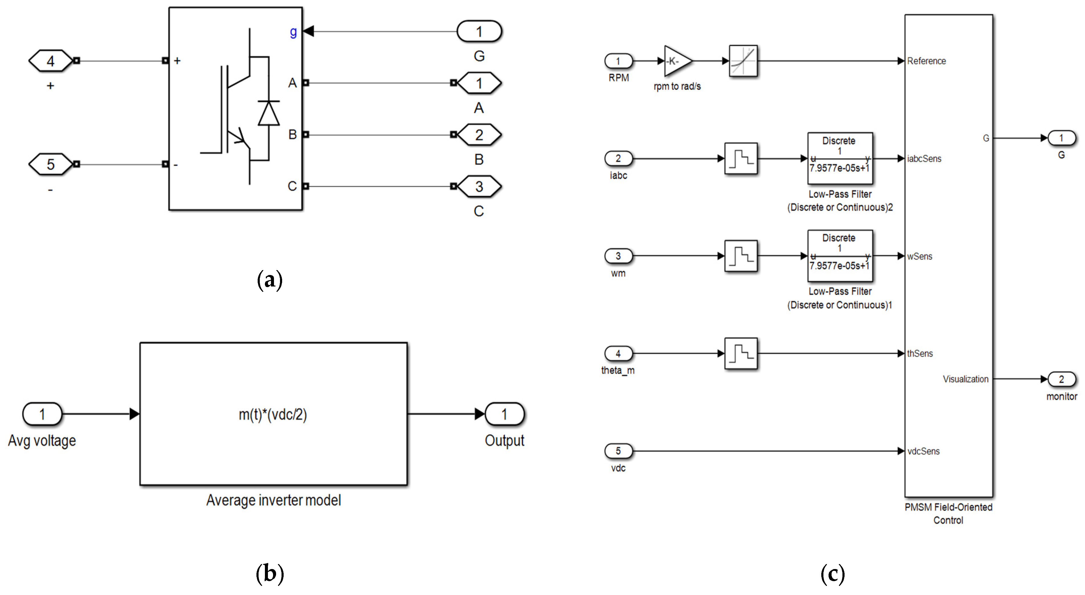
For the inverter, different modeling approaches were applied to the HFM and LFM. In the HFM, a universal bridge block was used to achieve modeling that was largely identical to that of the inverter installed on an actual ship. The inputs were the DC link voltage supplied by the battery system and the gate signals generated by the pulse width modulation (PWM) controller, while the output was the three-phase AC power supplied to the propulsion motor. Because the power semiconductor device used in a real ship is an insulated-gate bipolar transistor (IGBT), the power electronic device was set as the IGBT. In this case, the inverter was controlled using a PMSM field-oriented control block.

By contrast, in the LFM, an averaged inverter model was implemented using the PWM reference generator block. In the averaged model, the switching operation was not simulated, and the calculated three-phase voltage commands were used as the average voltages. Therefore, the high-frequency components related to switching cannot be represented, and analyses, such as total harmonic distortion (THD), are not feasible. However, the reduced-order inverter model used in this study preserved the essential operational characteristics, excluding the switching behavior, while reducing the computational cost and simulation time.

Next, the inverter controller was configured using the PMSM field-oriented control block. In this block, the proportional and integral gains of the speed controller were input into the external loop tab, whereas the proportional and integral gains of the d- and q-axis current controllers were input into the internal loop tab. In addition, the PWM tab was used to set the PWM method and switching frequency for the controller configuration separately. The controller transmits commands to the inverter to generate a specific voltage and frequency through which the inverter regulates the propulsion motor speed. In other words, the controller determines the voltage and frequency to be produced by the inverter, and the inverter adjusts the propulsion motor speed accordingly. Figure 6 shows the models of the inverter and inverter controllers.

The following equations represent the output voltage of the HFM inverter model and the average reference voltage of the LFM inverter model, respectively. Unlike the HFM model, which contains three switching functions, the LFM omits the switching operation, thereby reducing the computational burden. $v_{abc}\left(t\right)$ denotes the three-phase output voltage vector of the inverter, and $v_{dc}$ represents the DC-link voltage supplied to the inverter. $s_a\left(t\right),s_b\left(t\right)$, and $s_c\left(t\right)$ denote the switching functions of phases a, b, and c, respectively. Furthermore, $v_{abc}^{avg}\left(t\right)$ denotes the averaged three-phase output voltage vector of the inverter, and $m_{abc}\left(t\right)$ represents the modulation index vector for each phase, where $f(·)$ represents the nonlinear switching function that maps the DC-link voltage and switching states to the three-phase output voltages. The three-phase voltage vector is defined as $v_{abc}\left(t\right)={\left[v_a\left(t\right),v_b\left(t\right),v_c\left(t\right)\right]}^T$. The switching functions $s_a\left(t\right),s_b\left(t\right),s_c\left(t\right)$ are binary signals taking values of 0 or 1. The modulation index vector is defined as $m_{abc}\left(t\right)={\left[m_a\left(t\right),m_b\left(t\right),m_c\left(t\right)\right]}^T$.

$$v_{abc}\left(t\right)=f\left(v_{dc},s_a\left(t\right),s_b\left(t\right),s_c\left(t\right)\right)$$

(1)

$$v_{abc}^{avg}\left(t\right)=m_{abc}\left(t\right)·{\displaystyle \frac{v_{dc}}{2}}$$

(2)

The transfer function of the outer-loop speed controller of the inverter is defined as follows:

$$C_q\left(s\right)=K_{cq}\left(1+{\displaystyle \frac{1}{T_{iq}s}}\right)$$

(3)

The transfer function of the inner-loop current controller was applied identically to both the d- and q-axes.

$$C_s\left(s\right)=K_{cs}\left(1+{\displaystyle \frac{1}{T_{is}s}}\right)$$

(4)

$C_q\left(s\right)$ denotes the transfer function of the outer-loop speed controller, and $C_s\left(s\right)$ represents the transfer function of the inner-loop current controller. $K_{cq}$ and $K_{cs}$ are the proportional gains of the speed and current controllers, respectively, and $T_{iq}$ and $T_{is}$ denote their corresponding integral time constants. The current controller is applied identically to both the d- and q-axes. The variable $s$ is the Laplace variable representing the system dynamics.

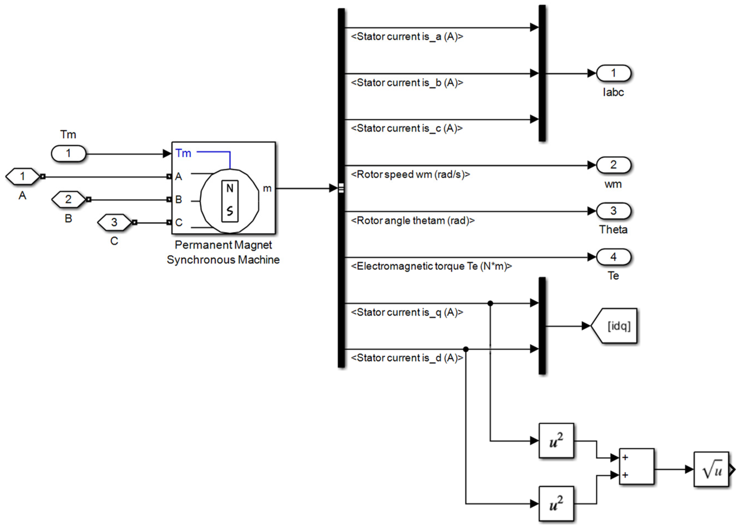
A PMSM block was used as the propulsion motor because the actual ship uses a PMSM. In the block parameter window, values, such as the rotor type, stator resistance, moment of inertia, and friction coefficient, were entered for the simulation. Figure 7 shows the propulsion motor model.

For the PMSM employed in the actual vessel, the following fundamental equations were considered, and the model was developed accordingly.

The following equations represent the d–q axis voltage equations:

$$v_d=R_s{i}_d+L_d{\displaystyle \frac{d{i}_d}{dt}}-{\omega }_e{L}_q{i}_q$$

(5)

$$v_q=R_s{i}_q+L_q{\displaystyle \frac{d{i}_q}{dt}}-{\omega }_e\left(L_d{i}_d+{\lambda }_{pm}\right)$$

(6)

The flux linkage can be formulated as follows:

$${\psi }_d=L_d{i}_d+{\lambda }_{pm},$$

(7)

$${\psi }_q=L_q{i}_q$$

(8)

The electromagnetic torque is defined by the following equation:

$$T_e={\displaystyle \frac{3}{2}}p\left({\lambda }_{pm}{i}_q+\left(L_d-L_q\right)i_d{i}_q\right)$$

(9)

The following expression describes the rotational dynamics:

$$J{\displaystyle \frac{{d\omega }_m}{dt}}=T_e-T_L-{B\omega }_m$$

(10)

The following equation represent the angular velocity transformation:

$${\omega }_e={p\omega }_m$$

(11)

$v_d$ and $v_q$ denote the d-axis and q-axis voltages, respectively, while $i_d$ and $i_q$ represent the d-axis and q-axis currents. $R_s$ is the stator resistance. $L_d$ and $L_q$ denote the d-axis and q-axis inductances, respectively, and ${\omega }_e$ represents the electrical angular speed.

${\lambda }_{pm}$ denotes the permanent magnet flux linkage. ${\psi }_d$ and ${\psi }_q$ represent the d-axis and q-axis flux linkages, respectively, which are determined by the currents and the permanent magnet flux. ${\displaystyle \frac{d{i}_d}{dt}}$ and ${\displaystyle \frac{d{i}_q}{dt}}$ denote the time derivatives of the d-axis and q-axis currents.

$T_e$ denotes the electromagnetic torque, which represents the torque generated by the motor. $p$ is the number of pole pairs. $J$ denotes the moment of inertia of the rotor, and ${\omega }_m$ represents the mechanical angular speed. $T_L$ denotes the load torque, and $B$ represents the viscous friction coefficient. The term ${B\omega }_m$ corresponds to the viscous friction torque. The phase currents are obtained from the inverse transformation of the d–q axis currents and are used as outputs of the propulsion motor model, where $t$ denotes time.

The block inputs were the three-phase power output from the inverter and the load torque obtained from ship dynamics. The block outputs included the phase currents of the propulsion motor, rotor angular speed, and motor output torque, which were transmitted to the inverter controller and monitoring system.

This study focused on a propulsion motor without a redundant structure using a digital twin model that considers fidelity. Because autonomous ships inherently operate in environments in which providing internal and external support is challenging, a loss of propulsion can lead to severe accidents. In particular, for certain ships wherein the propulsion motor is employed in a single-line configuration, failures may have more critical consequences compared with other components.

2.3. STEP 3—Failure Diagnosis Based on the Sliding-Window Approach

In Step 2, a digital twin model was constructed to simulate the nominal operating conditions of the actual ship. In this study, a fault was identified when the actual operating data deviated beyond a specific threshold from the simulated nominal data. For example, if the propulsion motor RPM decreased by more than 5% compared with the nominal state or if a sudden overload persisted for a specified duration, the condition was classified as a fault symptom. The condition of persistence for a specific duration was introduced to avoid misinterpreting the initial startup of the propulsion motor as a fault. During the initial start-up, known as the transient period, overcurrent inevitably occurs because of the characteristics of the motor. Because this is a natural phenomenon that occurs during normal operation, these conditions were excluded to prevent misclassification as faults.

This fault diagnosis approach is analogous to the process, wherein a ship engineer identifies abnormalities at an early stage by empirically assessing the current condition of the system. In conventional shipboard alarm monitoring systems (AMSs), abnormal condition is determined when a sensor measurement exceeds a predefined threshold. By contrast, the method proposed herein can play a critical role in terms of risk management. Risk management refers to identifying and analyzing potential hazards to minimize losses, which is consistent with the objectives of this study.

Consequently, a sliding-window technique was applied to the fault detection process. When applying this method, the window size must be set to ensure that temporary anomalies do not exert an excessive influence on the diagnostic results. Simultaneously, the window size should be adjusted to minimize the time delay associated with event detection. This approach allows trends to be identified by sufficiently reflecting past data within the data stream while maintaining balance so that essential data are not diluted by an excessive amount of information. Because the most recent data generally have the highest relevance, a sliding window provides an intuitive means of emphasizing them [52].

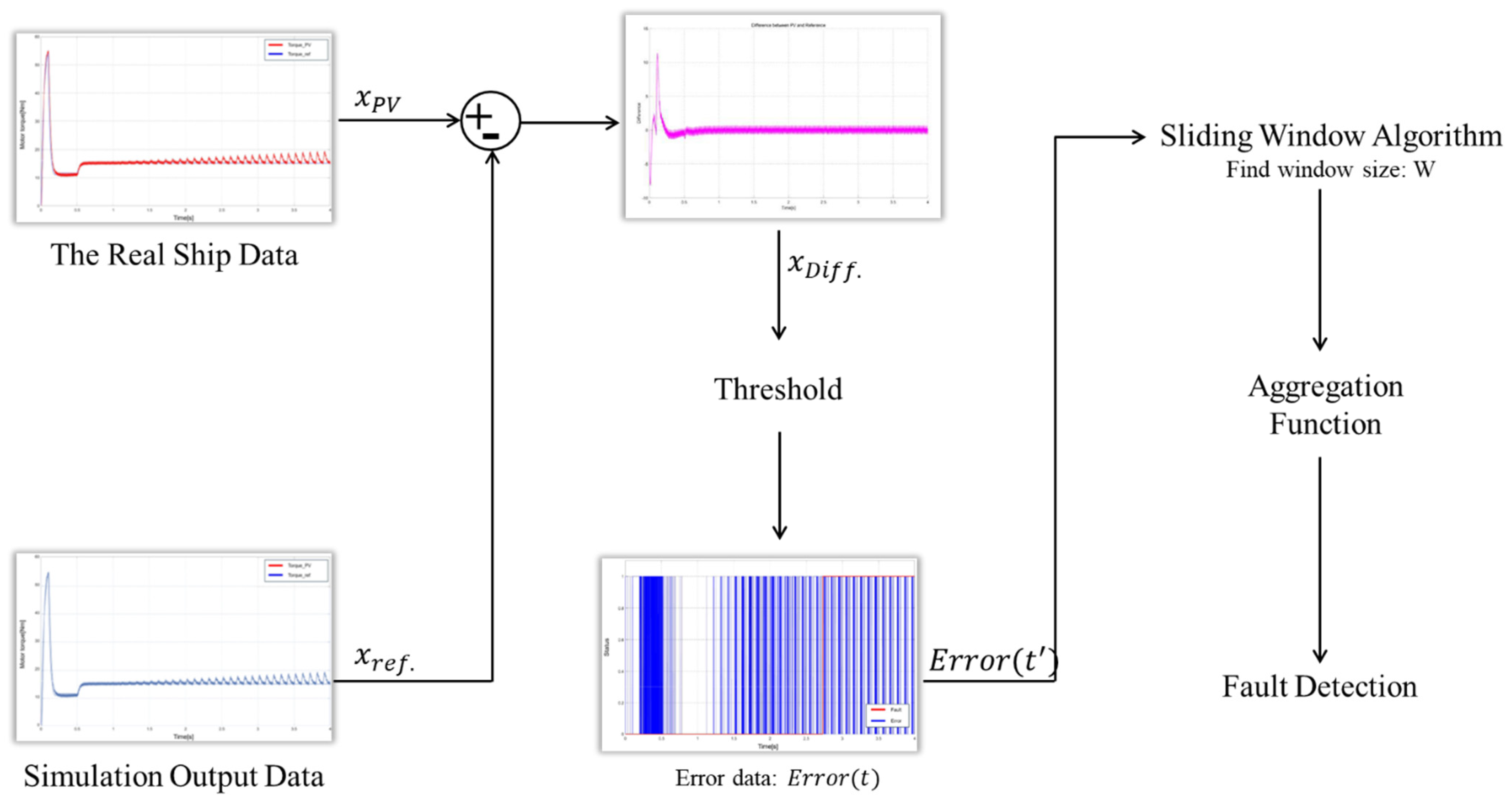
In the proposed fault diagnosis framework, algebraic aggregation functions, such as the average, were applied to ensure computational efficiency. Algebraic aggregation allows for the combination of multiple distributed aggregation functions (e.g., Sum, Count) to produce results, thereby enabling the representation of complex statistical values in a relatively simple form. This makes the proposed framework particularly suitable for real-time streaming data processing and sliding-window-based computation environments. In addition, it provides the advantage of efficiently calculating various statistical values such as the mean, standard deviation, geometric mean, and range. In this study, the Sum and Mean functions were used to diagnose different types of faults. Figure 8 presents an overview of Step 3.

Table 3. Parameters for Sliding Window-based Fault Diagnosis.

Symbol	Definition	Symbol	Definition
$\mathit{x}$	Original time-series data	${\mathit{y}}^{\left(\mathit{i}\right)}$	Aggregated output of window
$\mathit{W}$	Window length	$\mathit{\tau }$	Threshold for fault detection
$\mathit{s}$	Stride (step size for shifting the window)	${\widehat{\mathit{y}}}^{\left(\mathit{i}\right)}$	Predicted/expected outputted from the digital twin model
${\mathit{X}}^{\left(\mathit{i}\right)}$	Subsequence extracted at window starting index $i$	$\mathit{k}$	Repetition criterion
$\mathit{f}$	Aggregation function (e.g., sum, mean, max, min)	$\mathit{F}\mathit{a}\mathit{u}\mathit{l}\mathit{t}\left(\mathit{i}\right)$	Fault decision function

lists the parameters used to apply the sliding-window technique. In addition, the equations presented below show how the algebraic aggregation functions employed in the sliding-window method are utilized.

$$x=\left\{x_1,x_2,\dots ,x_T\right\}$$

(12)

$$X^{\left(i\right)}=\left\{x_i,x_{i+1},\cdots ,x_{i+W-1}\right\},i=1,1+s,1+2s,\cdots$$

(13)

For each window, an aggregation function $f$, such as Sum, Mean, Maximum, or Minimum, was applied to compute the corresponding value.

$$y^{\left(i\right)}=f\left(X^{\left(i\right)}\right)$$

(14)

$$Fault\left(i\right)=\left\{\begin{array}{c}1, if\left|y^{\left(i\right)}-{\widehat{y}}^{\left(i\right)}\right|>\tau \\ 0, otherwise \end{array}\right.$$

(15)

$$Fault\left(i\right)=\left\{\begin{array}{c}1, if{\sum }_{m=i}^{i+k-1}Fault\left(m\right)\ge k\\ 0, otherwise \end{array}\right.$$

(16)

2.4. STEP 4—Monitoring

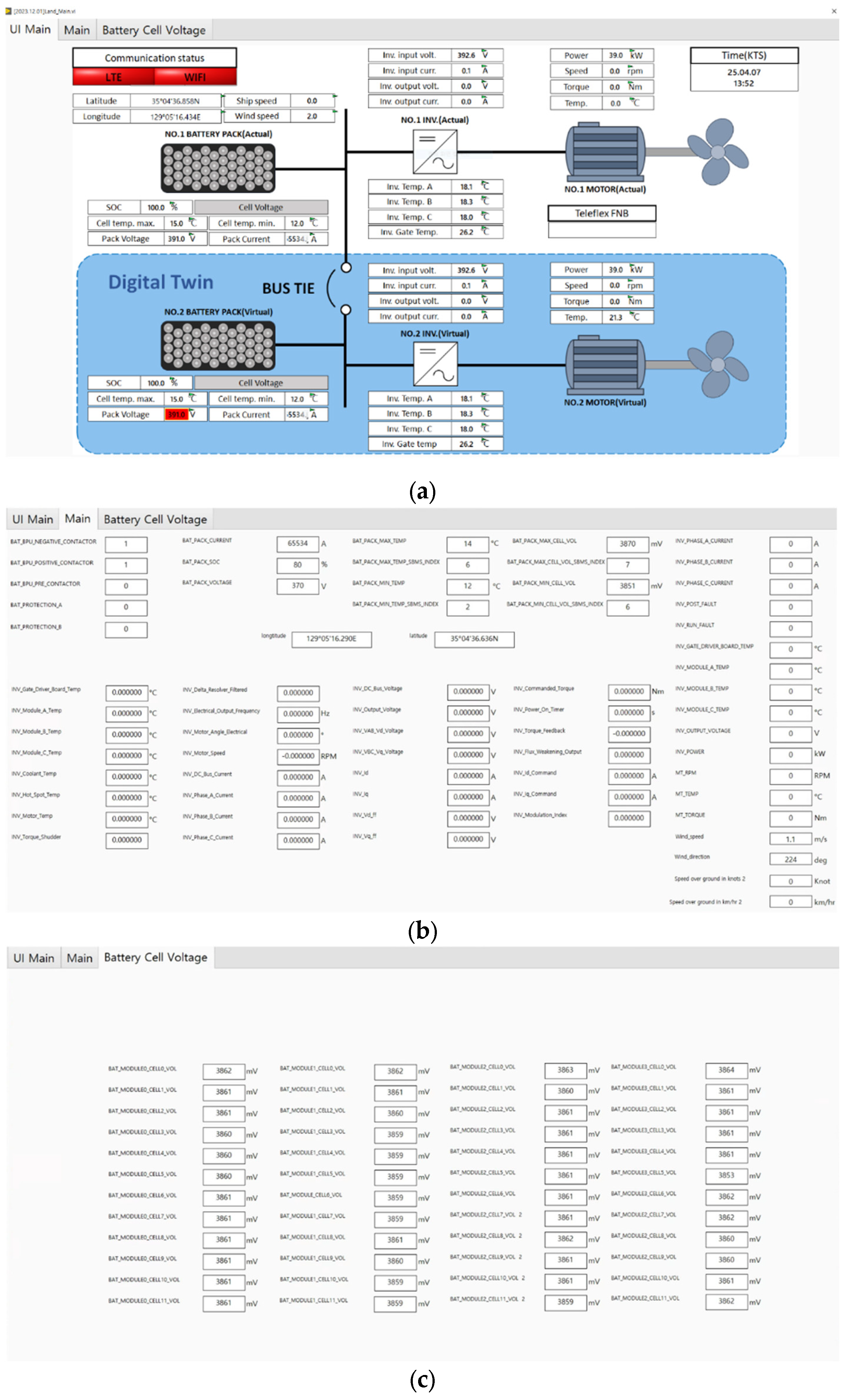
At the shore-based control center, the status of current, voltage, temperature, and other parameters transmitted from the actual ship via LTE can be monitored. The state of the digital twin model, which simulates the nominal conditions based on real ship data, can also be observed. This setup allows the present conditions to be checked and, by analyzing the error between the real ship and the digital twin model, faults can be detected. Actual data are continuously displayed, and when a fault occurs, the fault status is shown alongside the corresponding data.

Figure 9 shows the user interface (UI) of the integrated monitoring system linked with the digital twin, which enables real-time monitoring of the operating status of the ship from the shore-based control center. Here, (a) represents the main UI screen for checking the overall system status, (b) the main screen displaying the key operating data, and (c) the battery cell voltage screen for detailed monitoring of the cell voltage states.

3. Results

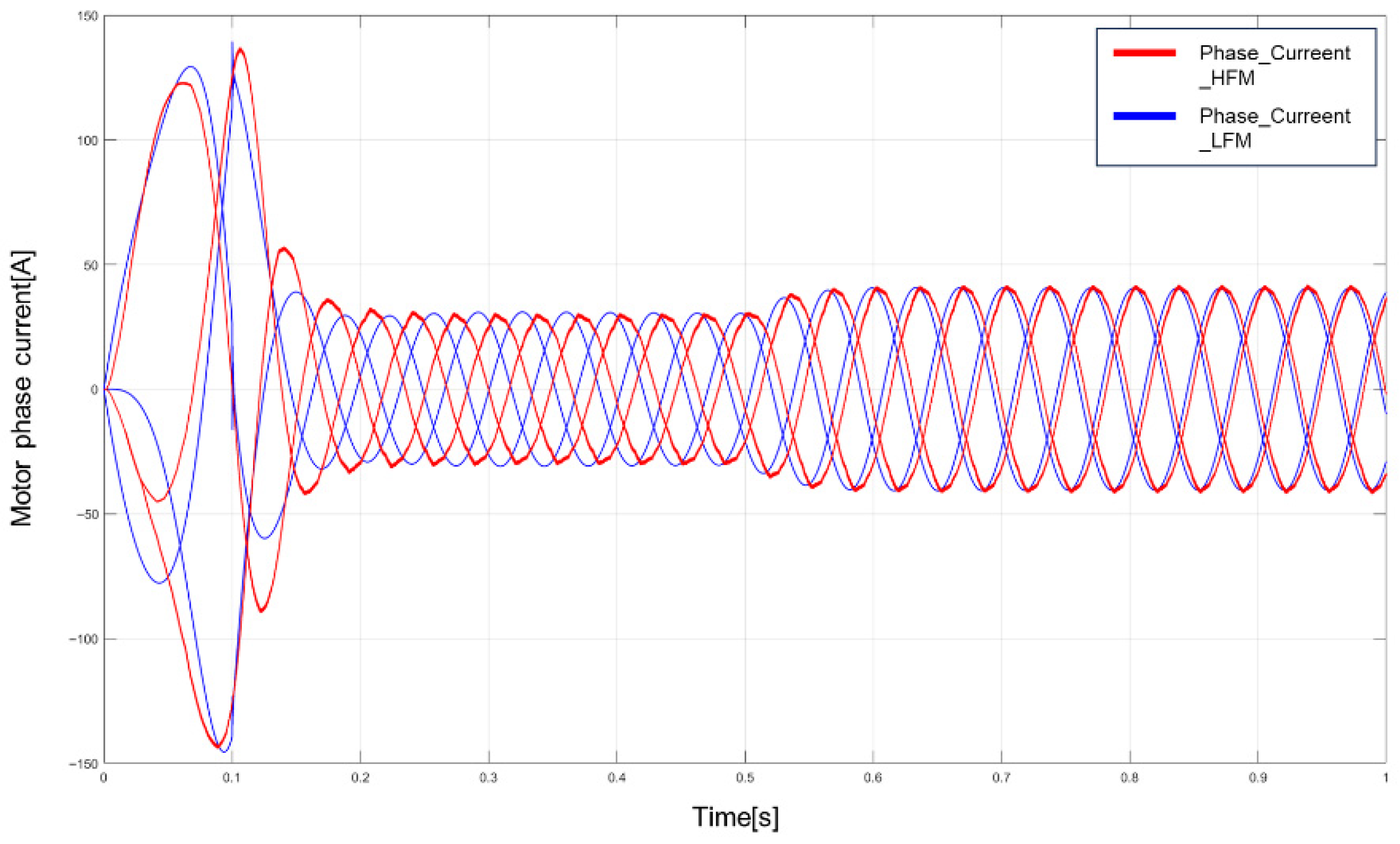
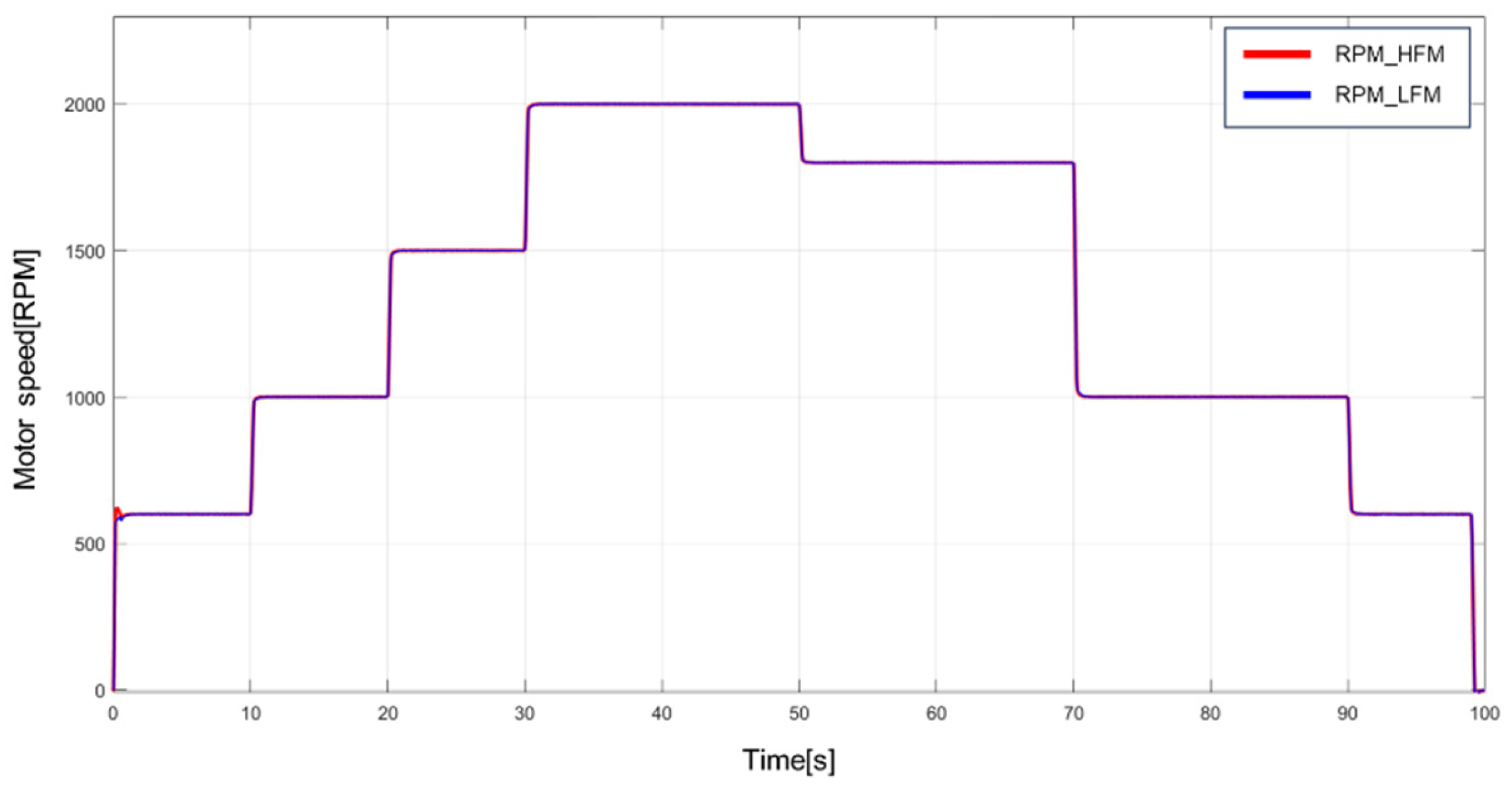
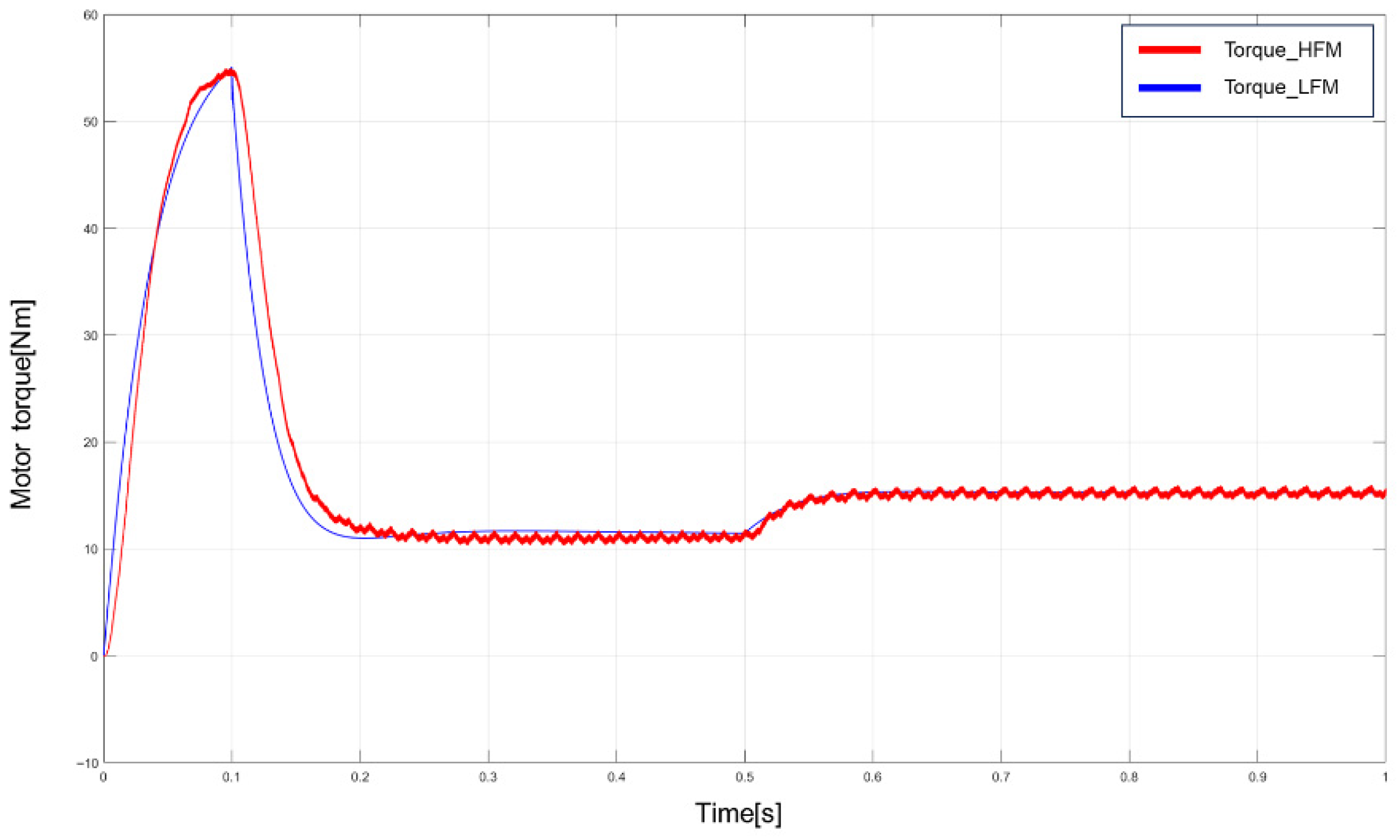
Prior to the fault diagnosis results, the operational characteristics of the HFM and LFM were verified under nominal conditions. The analysis confirmed that, except for the transient region, the system behaviors of the two models were nearly identical across most operating ranges. In addition, the HFM output included harmonic components resulting from the switching operations, and a torque ripple similar to that observed in the actual propulsion motor output. Figure 10, Figure 11 and Figure 12 respectively present the propulsion motor RPM of the HFM and LFM, propulsion motor output torque, and inverter output current.

To validate the proposed method, experiments were conducted on two fault modes that simulated fault data commonly occurring in electrical and mechanical systems.

In Case 1, a specific component of the system is assumed to be fixed in a damaged state or that it exhibits a certain degree of performance degradation. In this fault mode, the scenario of a rope being entangled around the propeller after the propulsion motor starts was considered. This represents a case wherein a sudden overload of constant magnitude is applied to the propeller or shaft, thereby creating a continuous deviation. The fault mode was evaluated by classifying the faults when the average error over a specific period exceeded 10% of the reference value.

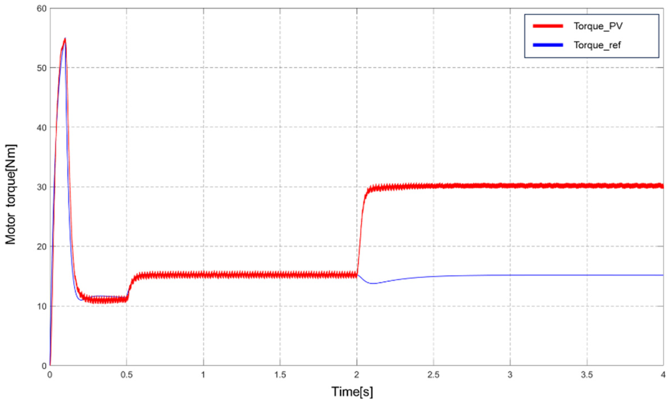
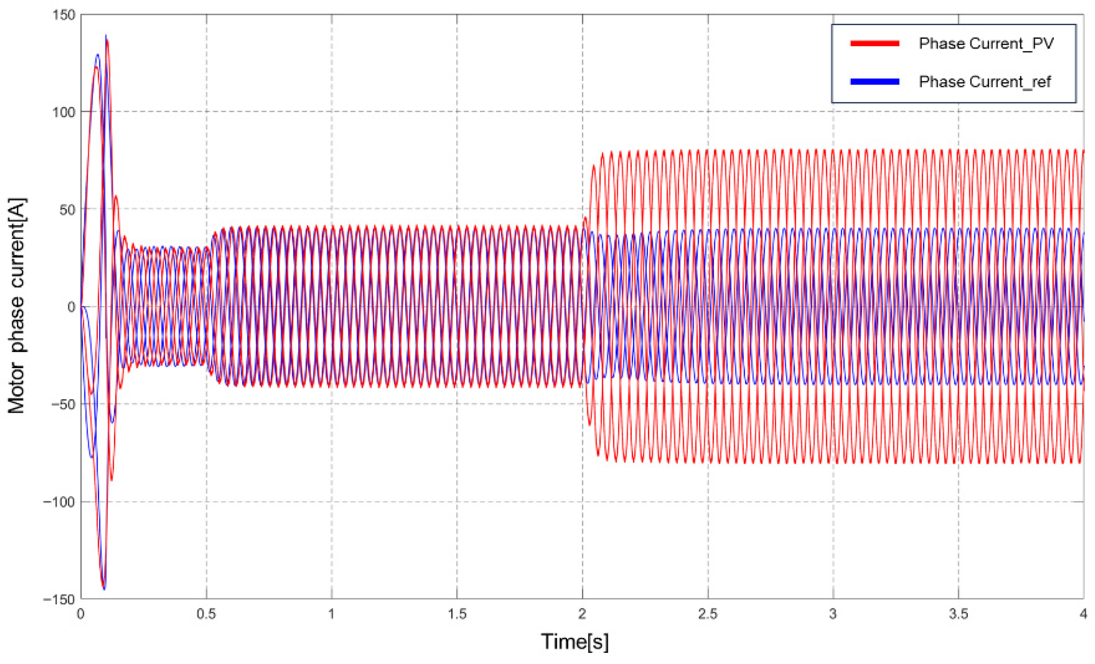
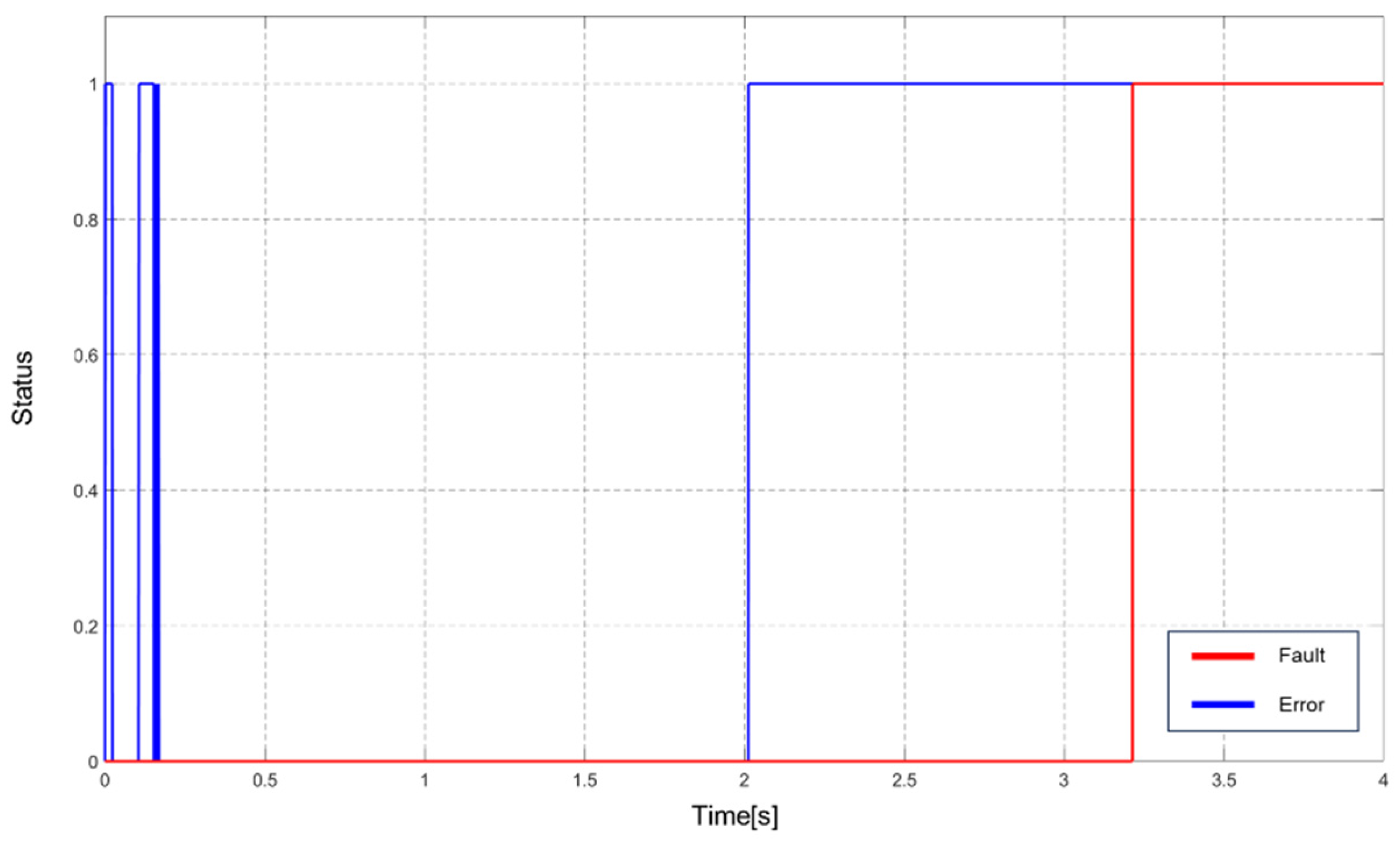
Figure 13 shows the onset of abnormal load torque, which occurs 2 s after the start of the simulation. Figure 14 confirms that an abnormal load current occurs simultaneously, also 2 s after the start of the simulation. Figure 15 shows that when the average error value within the sliding window exceeds a preset threshold, the condition is recognized as a fault. Although the system was in a transient state up to 0.5 s following startup, this was not classified as a fault. However, the error signal occurring at 2 s is recognized as a fault 1.2 s after its occurrence. This represents the optimal time for fault determination. The proposed approach exhibits behavior different from that of a conventional AMS, in which an abnormal condition is declared when the measured value exceeds the threshold for a specified duration.

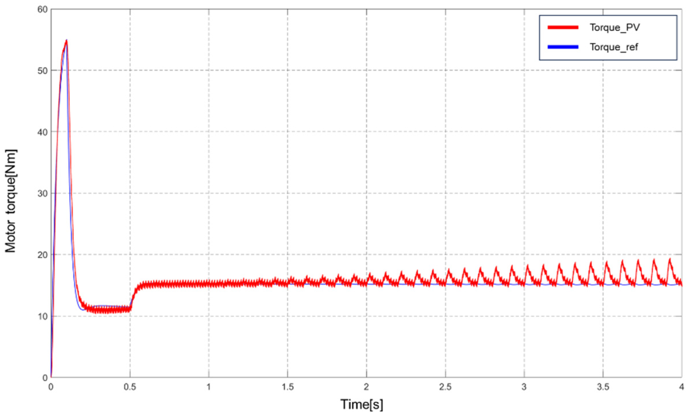
In Case 2, a fault is assumed, which is characterized by periodic oscillations that occur under a mechanical imbalance or cyclic load fluctuations. Unlike Case 1, in which a sudden overload occurred, this case did not exhibit distinct instantaneous changes in the measured values, making fault detection relatively more challenging. In this fault mode, an abnormal torque ripple with a constant period is assumed to occur after the propulsion motor starts, caused by issues such as bearing faults in the shaft system. This fault is characterized by a torque ripple whose error exceeds a specific proportion of the reference torque.

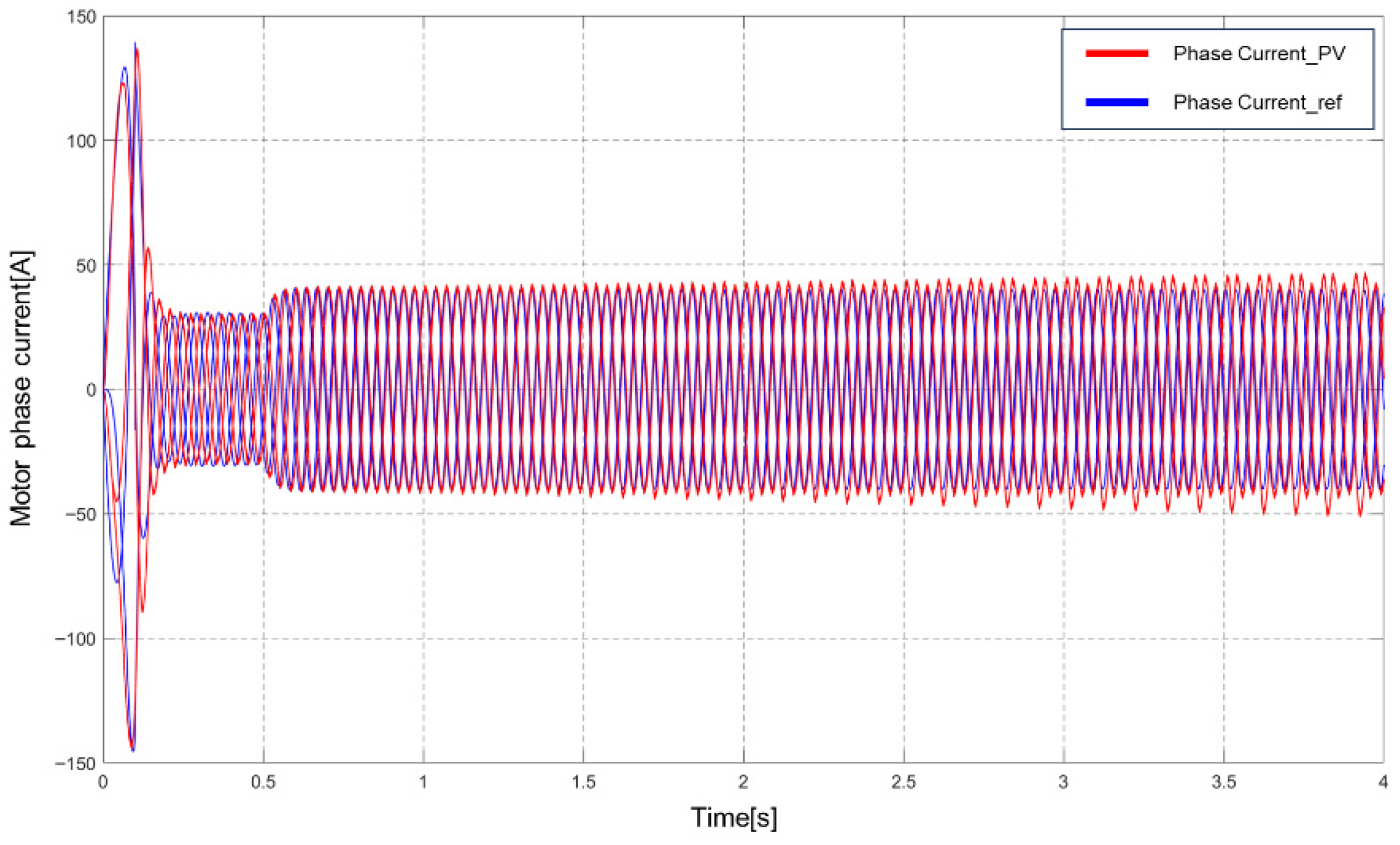
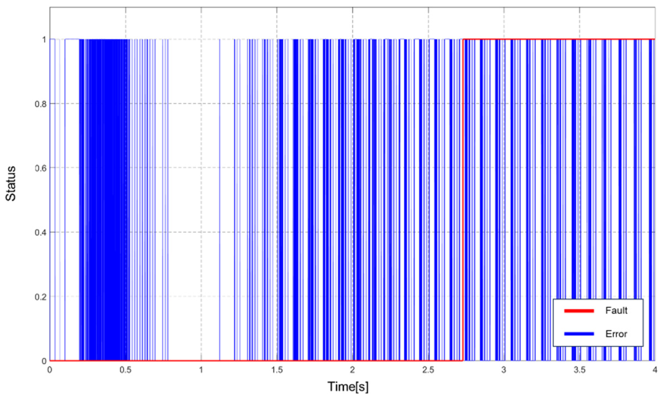
Figure 16 shows that an abnormal oscillating torque occurs after the start of the simulation. Figure 17 indicates that an abnormal load current has occurred under the same conditions. However, the deviation was minimal, with the current being only slightly higher than the reference phase current, making it difficult to clearly identify a fault. Nevertheless, Figure 18 shows that after passing through the transient state (approximately 0.5 s) following startup, a momentary error occurs at approximately 1.1 s, and the system subsequently detects the increase in error magnitude. From this point onward, the number of error occurrences within the sliding window was counted, and the fault was confirmed at approximately 2.7 s. This type of fault is challenging to detect using a conventional AMS, which can only identify faults when the threshold is exceeded for a specified duration and cannot detect faults characterized by periodic fluctuations.

4. Discussion

The validation was conducted employing a single vessel and a limited set of operating scenarios. Therefore, the performance may vary with different ship types or operational profiles. Furthermore, due to constraints on the number and placement of sensors, the sensitivity of observations to certain phenomena may have been insufficient, and additional validation is needed for environments with greater temporal variability. Finally, this study is limited by the fact that statistical optimization of the threshold settings was not performed.

Accordingly, future research directions must include extending the scope beyond propulsion motors to cover batteries, cooling systems, gear/shaft systems, and power converters with internal faults while also considering compound and multiple-fault scenarios. In addition, robust performance under changing environmental conditions could be achieved by introducing threshold automation based on receiver operating characteristic and precision–recall curve analyses, along with adaptive adjustment of the window length, stride, and repetition criteria. Nevertheless, the proposed approach is fundamentally based on a generic structure and procedure, which suggests that it can be applied to different vessel types (e.g., large merchant ships, passenger vessels, and small crafts) and a range of load conditions (e.g., diverse operating modes, load fluctuations, and sea states). This suggests that, despite the identified limitations, the method can be effectively extended to broader maritime applications.

This study presents a practical alternative for real-time fault monitoring by combining risk-based fidelity selection with lightweight real-time diagnosis, employing a simple and interpretable procedure for comparing real ship data with digital twin model outputs. The detection delays observed in Cases 1 and 2 demonstrate that the proposed method responded rapidly and reliably to distinct anomaly patterns. Further developments, such as threshold optimization, expansion of target systems, and validation in connection with standards, are expected to help extend this framework to an integrated digital-twin-based fault diagnosis system for autonomous ships, simultaneously enhancing both safety and operational efficiency.

5. Conclusions

This study developed a lightweight real-time fault diagnosis framework that selects model fidelity (HFM/LFM) based on the RPN obtained from the FMEA and employs a sliding-window technique. The proposed method was validated using real operating data with a sampling interval of 0.1 s, collected from an actual electric propulsion ship. Fault modes focused on the propulsion motor were simulated and linked with the corresponding digital twin model. The results confirmed that the proposed framework provides stable diagnostic performance that satisfies real-time monitoring requirements while reducing the reliance on computationally expensive learning-based artificial intelligence, thereby demonstrating its applicability to autonomous ships.

Employing RPN-based selective fidelity allocation, computational resources were concentrated on high-risk components, and the use of the mean deviation and repetition count within the sliding-window method enabled the efficient detection of continuous and periodic anomalies. In addition, the likelihood of false alarms was reduced by excluding the transient start-up period in advance and setting thresholds depending on the operating environment.

When the HFM is uniformly applied to all components, the real-time performance deteriorates, whereas the uniform application of the LFM results in the inability to capture detailed phenomena such as harmonics or ripples. The selective hybrid strategy proposed in this study achieved a balanced trade-off: HFMs were assigned to high-risk components to ensure diagnostic sensitivity, and LFMs were applied to low- and medium-risk areas to secure computational margins. Algebraic aggregation, based on the mean and count, demonstrated robustness even in streaming environments subject to communication delays and sensor noise. Furthermore, the simplicity of the proposed framework facilitated interpretation by operational and maintenance personnel. Compared with methods requiring large-scale learning and inference pipelines, this approach offers lower deployment and maintenance costs, along with improved interpretability.

In Case 1, a sudden and sustained overload condition was simulated, and a fault was declared when the mean deviation between the digital twin model and the actual ship exceeded a specified threshold owing to the rapid increase in the torque and current. The average detection delay was approximately 1.2 s. In Case 2, a periodic ripple caused by mechanical imbalance was simulated. To incorporate cases where a single threshold exceedance was minor, a repetition count was applied within the sliding window. In this case, the average detection delay was approximately 2.7 s, and the periodic ripple characteristics were stably detected without excessive false alarms. These results indicated that the proposed framework operated robustly against variability and noise in real-world data by addressing continuous-deviation-type anomalies (Case 1) and periodic anomalies (Case 2) using different aggregation rules.

References

1. Dukkanci, O.; Campbell, J.F.; Kara, B.Y. Facility location decisions for drone delivery: A literature review. Eur. J. Oper. Res. 2024, 316, 397–418. [Google Scholar] [CrossRef]
2. Souweidane, N.; Smith, B. State of ADAS, Automation, and Connectivity; Center for Automotive Research: Ann Arbor, MI, USA, 2023; pp. 1–40. [Google Scholar]
3. Zhang, X.; Sun, H.; Pei, X.; Guan, L.; Wang, Z. Evolution of technology investment and development of robotaxi services. Transp. Res. Part E 2024, 188, 103615. [Google Scholar] [CrossRef]
4. Maternová, A.; Materná, M.; Dávid, A.; Török, A.; Švábová, L. Human Error Analysis and Fatality Prediction in Maritime Accidents. J. Mar. Sci. Eng. 2023, 11, 2287. [Google Scholar] [CrossRef]
5. Bondarenko, O.; Fukuda, T. Development of a diesel engine’s digital twin for predicting propulsion system dynamics. Energy 2020, 196, 117126. [Google Scholar] [CrossRef]
6. Deon, B.; Cotta, K.P.; Silva, R.F.V.; Batista, C.B.; Justino, G.T.; Freitas, G.C.; Cordeiro, A.M.; Barbosa, A.S.; Loução, F.L.; Simioni, T.; et al. Digital twin and machine learning for decision support in thermal power plant with combustion engines. Knowl. Based Syst. 2022, 253, 109578. [Google Scholar] [CrossRef]
7. Malozemov, A.A.; Bondar, V.N.; Egorov, V.V.; Malozemov, G.A. Digital twins technology for internal combustion engines development. In Proceedings of the Global Smart Industry Conference (GloSIC); IEEE: New York, NY, USA, 2018; pp. 1–6. [Google Scholar] [CrossRef]
8. Söderäng, E.; Hautala, S.; Mikulski, M.; Storm, X.; Niemi, S. Development of a digital twin for real-time simulation of a combustion engine-based power plant with battery storage and grid coupling. Energy Convers. Manag. 2022, 266, 115793. [Google Scholar] [CrossRef]
9. Kaleem, M.B.; He, W.; Li, H. Machine learning driven digital twin model of Li-ion batteries in electric vehicles: A review. Artif. Intell. Auton. Syst. 2023, 1, 0003. [Google Scholar] [CrossRef]
10. Li, W.; Rentemeister, M.; Badeda, J.; Jöst, D.; Schulte, D.; Sauer, D.U. Digital twin for battery systems: Cloud battery management system with online state-of-charge and state-of-health estimation. J. Energy Storage 2020, 30, 101557. [Google Scholar] [CrossRef]
11. International Maritime Organization (IMO). MASS Code: Maritime Autonomous Surface Ships Code, London, UK, 2023. Available online: https://buly.kr/APvdfM1 (accessed on 22 February 2026).
12. Menis, R.; da Rin, A.; Vicenzutti, A.; Sulligoi, G. Dependable design of all electric ships integrated power system: Guidelines for system decomposition and analysis. In Proceedings of the Electrical Systems for Aircraft, Railway and Ship Propulsion; IEEE: New York, NY, USA, 2012; pp. 1–6. [Google Scholar] [CrossRef]
13. Bai, H.; Yu, B. Position estimation of fault-tolerant permanent magnet motor in electric power propulsion ship system. IEEJ Trans. Electr. Electron. Eng. 2022, 17, 890–898. [Google Scholar] [CrossRef]
14. Lee, J.H.; Park, S.K.; Bazher, S.A.; Seo, D. Development of a fault prediction algorithm for marine propulsion energy storage system. Energies 2025, 18, 1687. [Google Scholar] [CrossRef]
15. Xie, J.; Shi, W.; Shi, Y. Research on fault diagnosis of six-phase propulsion motor drive inverter for marine electric propulsion system based on Res-BiLSTM. Machines 2022, 10, 736. [Google Scholar] [CrossRef]
16. Tao, F.; Zhang, H.; Liu, A.; Nee, A.Y.C. Digital twin in industry: State-of-the-art. IEEE Trans. Ind. Inform. 2019, 15, 2405–2415. [Google Scholar] [CrossRef]
17. Ríos, J.; Staudter, G.; Weber, M.; Anderl, R. Enabling the digital twin: A review of the modelling of measurement uncertainty on data transfer standards and its relationship with data from tests. Int. J. Prod. Lifecycle Manag. 2020, 12, 250–268. [Google Scholar] [CrossRef]
18. Melesse, T.Y.; Pasquale, V.D.; Riemma, S. Digital twin models in industrial operations: A systematic literature review. Procedia Manuf. 2020, 42, 267–272. [Google Scholar] [CrossRef]
19. Tao, F.; Xiao, B.; Qi, Q.; Cheng, J.; Ji, P. Digital twin modeling. J. Manuf. Syst. 2022, 64, 372–389. [Google Scholar] [CrossRef]
20. Desai, A.S.; Navaneeth, N.; Adhikari, S.; Chakraborty, S. Enhanced multi-fidelity modeling for digital twin and uncertainty quantification. Probab. Eng. Mech. 2023, 74, 103525. [Google Scholar] [CrossRef]
21. Xu, Z.; Gao, T.; Li, Z.; Bi, Q.; Liu, X.; Tian, K. Digital twin modeling method for hierarchical stiffened plate based on transfer learning. Aerospace 2023, 10, 66. [Google Scholar] [CrossRef]
22. Kontaxoglou, A.; Tsutsumi, S.; Khan, S.; Nakasuka, S. Towards a digital twin enabled multifidelity framework for small satellites. In PHM Society European Conference; PHM Society: Rochester, NY, USA, 2021; Volume 6, p. 10. [Google Scholar] [CrossRef]
23. Mutlu, N.G.; Altuntas, S. Risk analysis for occupational safety and health in the textile industry: Integration of FMEA, FTA, and BIFPET methods. Int. J. Ind. Ergon. 2019, 72, 222–240. [Google Scholar] [CrossRef]
24. International Electrotechnical Commission (IEC). IEC; Fault Tree Analysis (FTA): Geneva, Switzerland, 2006; Available online: https://buly.kr/4xY9G5X (accessed on 3 March 2026).
25. Ahn, J.; Chang, D. Fuzzy-based HAZOP study for process industry. J. Hazard. Mater. 2016, 317, 303–311. [Google Scholar] [CrossRef]
26. de la O Herrera, M.A.; Luna, A.S.; da Costa, A.C.A.; Lemes, E.M.B. Risk analysis: A generalized Hazop methodology state-of-the-art, applications, and perspective in the process industry. Vigil. Sanit. Debate Soc. Cienc. Tecnol. 2018, 6, 106–121. [Google Scholar] [CrossRef]
27. Wu, J.; Lind, M. Management of system complexity in hazop for the oil & gas industry. IFAC PapersOnLine 2018, 51, 211–216. [Google Scholar] [CrossRef]
28. Penelas, A.J.; Pires, J.C.M. Hazop analysis in terms of safety operations processes for oil production units: A case study. Appl. Sci. 2021, 11, 10210. [Google Scholar] [CrossRef]
29. Nuchpho, P.; Nansaarng, S.; Pongpullponsak, A. Risk assessment in the organization by using FMEA innovation: A literature review. In Proceedings of the 7th International Conference on Education Reform; Industry Council for Electronic Equipment Recycling: London, UK, 2014; pp. 781–789. [Google Scholar]
30. Paciarotti, C.; Mazzuto, G.; D’Ettorre, D. A revised FMEA application to the quality control management. Int. J. Qual. Rel. Manag. 2014, 31, 788–810. [Google Scholar] [CrossRef]
31. Goddard, P.L. Software FMEA techniques. In Proceedings of the Annual Reliability and Maintainability Symposium; IEEE: New York, NY, USA, 2000; pp. 118–123. [Google Scholar] [CrossRef]
32. Feili, H.R.; Akar, N.; Lotfizadeh, H.; Bairampour, M.; Nasiri, S. Risk analysis of geothermal power plants using failure modes and effects analysis (FMEA) technique. Energy Convers. Manag. 2013, 72, 69–76. [Google Scholar] [CrossRef]
33. Subriadi, A.P.; Najwa, N.F. The consistency analysis of failure mode and effect analysis (FMEA) in information technology risk assessment. Heliyon 2020, 6, e03161. [Google Scholar] [CrossRef]
34. Jain, K. Use of failure mode effect analysis (FMEA) to improve medication management process. Int. J. Health Care Qual. Assur. 2017, 30, 175–186. [Google Scholar] [CrossRef]
35. Mascia, A.; Cirafici, A.M.; Bongiovanni, A.; Colotti, G.; Lacerra, G.; Di Carlo, M.; Digilio, F.A.; Liguori, G.L.; Lanati, A.; Kisslinger, A. A failure mode and effect analysis (FMEA)-based approach for risk assessment of scientific processes in non-regulated research laboratories. Accredit. Qual. Assur. 2020, 25, 311–321. [Google Scholar] [CrossRef]
36. Filz, M.A.; Langner, J.E.B.; Herrmann, C.; Thiede, S. Data-driven failure mode and effect analysis (FMEA) to enhance maintenance planning. Comput. Ind. 2021, 129, 103451. [Google Scholar] [CrossRef]
37. Baig, S.R.; Iqbal, W.; Berral, J.L.; Carrera, D. Adaptive sliding windows for improved estimation of data center resource utilization. Future Gener. Comput. Syst. 2020, 104, 212–224. [Google Scholar] [CrossRef]
38. Peng, H.; Huang, S.; Chen, S.; Li, B.; Geng, T.; Li, A.; Jiang, W.; Wen, W.; Bi, J.; Liu, H.; et al. A length adaptive algorithm-hardware co-design of transformer on FPGA through sparse attention and dynamic pipelining. In Proceedings of the 59th ACM IEEE Design Automation Conference; Association for Computing Machinery: New York, NY, USA, 2022; pp. 1135–1140. [Google Scholar] [CrossRef]
39. Bifet, A.; Gavaldà, R. Learning from time-changing data with adaptive windowing. In Proceedings of the SIAM International Conference on Data Mining; Society for Industrial and Applied Mathematics: Philadelphia, PA, USA, 2007; pp. 443–448. [Google Scholar] [CrossRef]
40. Kshirasagar, S.; Guntoro, A.; Mayr, C. Impact of sliding window variation and neuronal time constants on acoustic anomaly detection using recurrent spiking neural networks in automotive environment. Algorithms 2024, 17, 440. [Google Scholar] [CrossRef]
41. Schmidl, S.; Wenig, P.; Papenbrock, T. Anomaly detection in time series: A comprehensive evaluation. Proc. VLDB Endow. 2022, 15, 1779–1797. [Google Scholar] [CrossRef]
42. Kulanuwat, L.; Chantrapornchai, C.; Maleewong, M.; Wongchaisuwat, P.; Wimala, S.; Sarinnapakorn, K.; Boonya-aroonnet, S. Anomaly detection using a sliding window technique and data imputation with machine learning for hydrological time series. Water 2021, 13, 1862. [Google Scholar] [CrossRef]
43. Issa, R.; Badr, M.M.; Shalash, O.; Othman, A.A.; Hamdan, E.; Hamad, M.S.; Abdel-Khalik, A.S.; Ahmed, S.; Imam, S.M. A data-driven digital twin of electric vehicle Li-ion battery state-of-charge estimation enabled by driving behavior application programming interfaces. Batteries 2023, 9, 521. [Google Scholar] [CrossRef]
44. Costa, M.; Del Papa, G. Digital Twins for Intelligent Vehicle-to-Grid Systems: A Multi-Physics EV Model for AI-Based Energy Management. Appl. Sci. 2025, 15, 8214. [Google Scholar] [CrossRef]
45. Feng, K.; Xu, Y.; Wang, Y.; Li, S.; Jiang, Q.; Sun, B.; Zheng, J.; Ni, Q. Digital Twin Enabled Domain Adversarial Graph Networks for Bearing Fault Diagnosis. IEEE Trans. Ind. Cyber-Phys. Syst. 2023, 1, 113–122. [Google Scholar] [CrossRef]
46. Yang, C.; Cai, B.; Wu, Q.; Wang, C.; Ge, W.; Hu, Z.; Zhu, W.; Zhang, L.; Wang, L. Digital twin-driven fault diagnosis method for composite faults by combining virtual and real data. J. Ind. Inf. Integr. 2023, 33, 100469. [Google Scholar] [CrossRef]
47. Xia, J.; Huang, R.; Chen, Z.; He, G.; Li, W. A novel digital twin-driven approach based on physical-virtual data fusion for gearbox fault diagnosis. Reliab. Eng. Syst. Saf. 2023, 240, 109542. [Google Scholar] [CrossRef]
48. Xia, J.; Huang, R.; Li, J.; Chen, Z.; Li, W. Digital Twin-Assisted Fault Diagnosis of Rotating Machinery Without Measured Fault Data. IEEE Trans. Instrum. Meas. 2024, 73, 3531210. [Google Scholar] [CrossRef]
49. Qin, Y.; Liu, H.; Mao, Y. Faulty Rolling Bearing Digital Twin Model and Its Application in Fault Diagnosis with Imbalanced Samples. Adv. Eng. Inform. 2024, 61, 102513. [Google Scholar] [CrossRef]
50. Xia, J.; Chen, Z.; Chen, J.; He, G.; Huang, R.; Li, W. A Digital Twin-Driven Approach for Partial Domain Fault Diagnosis of Rotating Machinery. Eng. Appl. Artif. Intell. 2024, 131, 107848. [Google Scholar] [CrossRef]
51. Huang, Y.; Tao, J.; Sun, G.; Wu, T.; Yu, L.; Zhao, X. A novel digital twin approach based on deep multimodal information fusion for aero-engine fault diagnosis. Energy 2023, 270, 126894. [Google Scholar] [CrossRef]
52. Bo, Y.; Wu, H.; Che, W.; Zhang, Z.; Li, X.; Myagkov, L. Methodology and application of digital twin-driven diesel engine fault diagnosis and virtual fault model acquisition. Eng. Appl. Artif. Intell. 2024, 131, 107853. [Google Scholar] [CrossRef]
53. Kodosky, J. LabVIEW. Proc. ACM Program. Lang. 2020, 4, 78. [Google Scholar] [CrossRef]
54. Ceylan, B.O. Shipboard compressor system risk analysis by using rule-based fuzzy FMEA for preventing major marine accidents. Ocean Eng. 2023, 272, 113888. [Google Scholar] [CrossRef]
55. Hwang, S.K.; Kim, D.H.; Kim, S.C. Analysis of risk priority number of FMEA and surprise index for components of 7 kW electric vehicle charger. J. Loss Prev. Process Ind. 2024, 91, 105375. [Google Scholar] [CrossRef]
56. Garcia, P.A.A.; Schirru, R.; Frutuoso E^Melo, P.F. A fuzzy data envelopment analysis approach for FMEA. Prog. Nucl. Energy 2005, 46, 359–373. [Google Scholar] [CrossRef]
57. Xiao, N.; Huang, H.Z.; Li, Y.; He, L.; Jin, T. Multiple failure modes analysis and weighted risk priority number evaluation in FMEA. Eng. Fail. Anal. 2011, 18, 1162–1170. [Google Scholar] [CrossRef]
58. Chang, K.-H. Evaluate the orderings of risk for failure problems using a more general RPN methodology. Microelectron. Reliab. 2009, 49, 1586–1596. [Google Scholar] [CrossRef]
59. Chen, K.; Kurgan, L.; Ruan, J. Optimization of the sliding window size for protein structure prediction. In Proceedings of the IEEE Symposium on Computational Intelligence and Bioinformatics and Computational Biology (CIBCB); IEEE: New York, NY, USA, 2006; pp. 1–7. [Google Scholar] [CrossRef]
Figure 1. Overview of the proposed fault diagnosis method with fidelity selection.
Machines 14 00480 g001
Figure 2. Operation of an electric propulsion vessel: (a) CCTV footage; (b) Voyage track (Busan Port).
Machines 14 00480 g002
Figure 3. Configuration of the network stream system in the 100 kW electric propulsion ship.
Machines 14 00480 g003
Figure 4. Selection of fidelity model based on risk priority number (RPN).
Machines 14 00480 g004
Figure 5. Configuration of battery system.
Machines 14 00480 g005
Figure 6. Configuration of inverter: (a) Inverter; (b) Averaged model inverter; (c) Controller for inverter.
Machines 14 00480 g006
Figure 7. Configuration of propulsion motor control.
Machines 14 00480 g007
Figure 8. Flowchart of fault detection using sliding window.
Machines 14 00480 g008
Figure 9. User interface (UI) of integrated monitoring system connected to the digital twin: (a) UI Main; (b) Main; (c) Battery cell voltage.
Machines 14 00480 g009
Figure 10. Simulation results of propulsion motor speed (RPM) under nominal condition.
Machines 14 00480 g010
Figure 11. Simulation results of propulsion motor output torque under nominal condition.
Machines 14 00480 g011
Figure 12. Simulation results of inverter output current under nominal condition.
Machines 14 00480 g012
Figure 13. Case 1—Results of propulsion motor output torque under entanglement fault condition.
Machines 14 00480 g013
Figure 14. Case 1—Results of propulsion motor phase current under entanglement fault condition.
Machines 14 00480 g014
Figure 15. Case 1—Results of fault detection under entanglement fault condition.
Machines 14 00480 g015
Figure 16. Case 2—Results of propulsion motor output torque under periodic load fluctuation.
Machines 14 00480 g016
Figure 17. Case 2—Results of propulsion motor phase current under periodic load fluctuation.
Machines 14 00480 g017
Figure 18. Case 2—Results of fault detection under periodic load fluctuation.
Machines 14 00480 g018