An Ensemble-LSTM-Based Framework for Improved Prognostics and Health Management of Milling Machine Cutting Tools

Abstract

Accurate Prognostics and Health Management (PHM) of cutting tools in Computer Numerical Control (CNC) milling machines is essential for minimizing downtime, improving product quality, and reducing maintenance costs. Previous studies have frequently applied deep learning, particularly Long Short-Term Memory (LSTM) neural networks, for tool wear prediction and Remaining Useful Life (RUL) prediction. However, they often rely on simplified datasets or single architectures limiting industrial relevance. This study proposes a novel ensemble-LSTM framework that combines LSTM, BiLSTM, Stacked LSTM, and Stacked BiLSTM architectures using a GRU-based meta-learner to exploit their complementary strengths. The framework is evaluated using the publicly available PHM’2010 milling dataset, a well-established industrial benchmark comprising comprehensive time-series sensor measurements collected under variable loads and realistic machining conditions. Experimental results show that the ensemble-LSTM outperforms individual LSTM models, achieving an RMSE of 2.4018 and an MAE of 1.9969, accurately capturing progressive tool wear trends and adapting to unseen operating conditions. The approach provides a robust, reliable solution for real-time predictive maintenance and demonstrates strong potential for industrial tool condition monitoring.

1. Introduction

Milling machines represent the cornerstone of modern manufacturing infrastructure, serving as critical enablers in precision-dependent industries including aerospace, automotive, defense, and medical device manufacturing [1]. These sophisticated machine tools facilitate the complex shaping of metallic and composite materials through material removal processes, where their operational efficiency directly correlates with product quality, production throughput, and overall manufacturing competitiveness [2].

The operational environment of milling machine cutting tools constitutes one of the most challenging scenarios in manufacturing engineering [3]. Cutting tools are subjected to extreme thermo-mechanical stresses during metal removal operations, experiencing complex interactions of cutting forces, high temperatures at the tool–work-piece interface, and cyclic mechanical loading that induces progressive wear mechanisms [4]. These harsh operating conditions trigger multiple wear phenomena including abrasive wear, adhesive wear, and thermal cracking, collectively contributing to the gradual degradation of cutting tool integrity and performance [5].

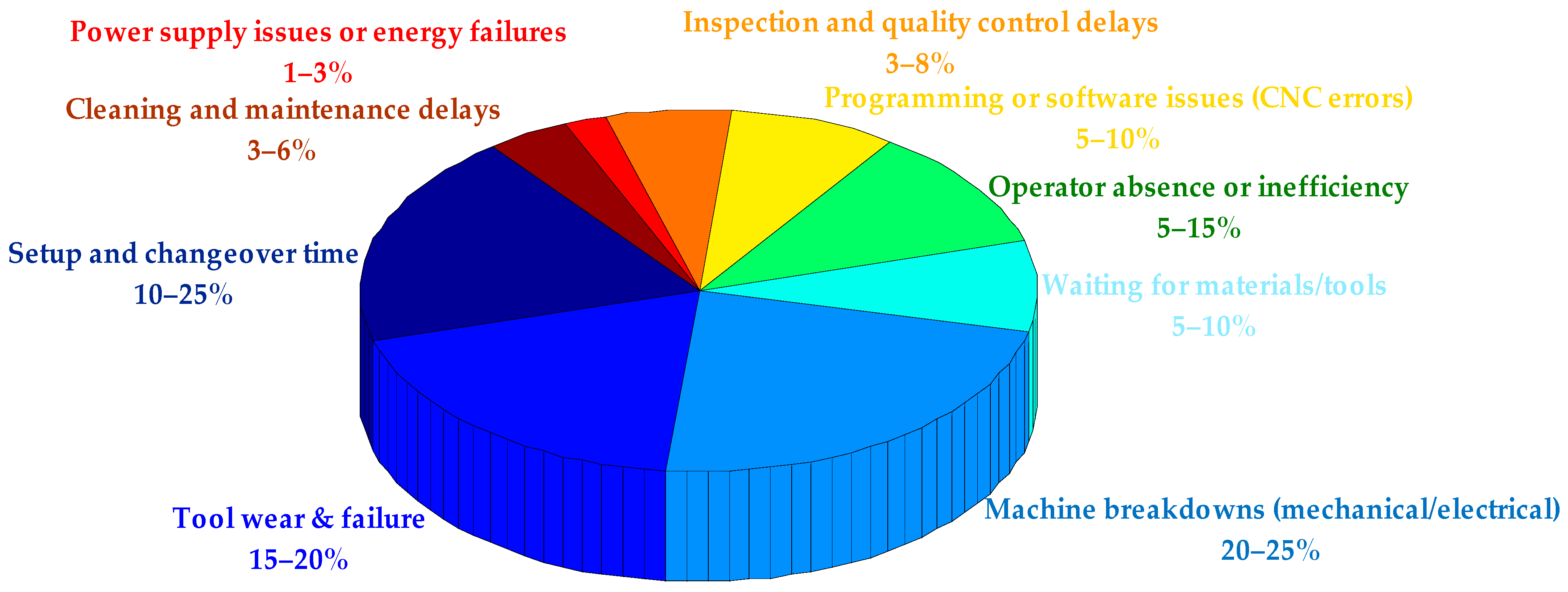
The economic implications of cutting tool performance extend far beyond simple replacement costs [6]. Modern cutting tools and the work-piece materials being machined, often expensive aerospace alloys or sophisticated composites, carry substantial value. As shown in Figure 1, industry studies indicate that tool wear-related issues account for approximately 15–20% of total machine tool downtime in manufacturing facilities. In addition, unexpected tool changes contribute to 3–12% of total manufacturing costs in precision machining operations [7]. This suggests that nearly 1/5 of all downtime could potentially be mitigated with better tool wear monitoring, predictive maintenance, or improved cutting tool materials/coatings. Also, it presents a major cost driver, especially in high-precision environments where tolerances are tight, and downtime or scrap from sudden tool failure can be expensive.

Beyond direct economic impacts, tool degradation manifests in multiple detrimental effects on manufacturing outcomes. Progressive tool wear directly influences surface finish quality, dimensional accuracy, and geometrical tolerances of machined components [8]. Furthermore, worn tools significantly increase energy consumption due to increased cutting forces and reduced machining efficiency [9]. In severe cases, undetected tool wear can progress to catastrophic tool failure, potentially causing collateral destruction to the machine tool components and consequently to the work-piece [10].

The emergence of Prognostics and Health Management (PHM) as a systematic engineering discipline has transformed approaches to manufacturing equipment maintenance and reliability [11]. PHM represents a paradigm shift from traditional maintenance strategies toward predictive methodologies that enable condition-based maintenance decisions. In milling operations, PHM systems aim to predict accurately the Remaining Useful Life (RUL) of cutting tools, thereby optimizing tool utilization and minimizing unplanned downtime [12].

Considering the open literature, two principal methodological frameworks dominate PHM implementation for tool condition monitoring. Model-based approaches leverage physical principles and mathematical models to simulate tool degradation processes [13]. While offering valuable insights into fundamental wear mechanisms, these methods often struggle with the complex, nonlinear nature of tool wear progression under varying operational conditions [14]. Data-driven approaches utilize operative data recorded through sensor systems to model tool health without explicit physical modeling [15]. The proliferation of advanced sensor technologies has enabled comprehensive data collection during machining operations. Data-driven methods excel at capturing complex patterns from multivariate sensor data and adapting to specific operational contexts [16]. Within the data-driven paradigm, machine learning and deep learning techniques have demonstrated significant abilities in tool wear prediction [17]. As shown in

Table 1. Comparative overview of data-driven methods for CNC tool wear prediction.

Method	Key Advantages	Limitations	Typical Performance	References
SVM	Effective in high-dimensional spaces; Strong generalization	Requires feature engineering; Limited temporal modeling	RMSE: 8–15 μm; R2: 0.75–0.88	[21,22]
ANN	Models complex nonlinear relationships; Adaptable to sensors	Prone to overfitting; Extensive tuning required	RMSE: 7–12 μm; R2: 0.80–0.90	[23,24]
BiLSTM	Comprehensive contextual understanding; Superior temporal patterns	High computational requirements; Longer training	RMSE: 5–9 μm; R2: 0.88–0.95	[25,26]
GRU	Faster training convergence; Reduced computational load	Less validation compared to LSTM	RMSE: 6–10 μm; R2: 0.85–0.92	[27,28]
LSTM	Proven long-term dependency modeling; Flexible architecture	Sensitive to hyperparameters; Requires large data	RMSE: 5–8 μm; R2: 0.87–0.94	[29,30]

, traditional algorithms of machine learning such as Support Vector Machines (SVM) and Artificial Neural Networks (ANN) have been extensively applied, but these approaches typically require significant manual feature engineering and may lack temporal modeling capabilities [18]. This table summarizes key data-driven approaches for tool wear prediction, including model types, key advantages, limitations, and reported performance metrics (e.g., RMSE, MAE). It highlights the strengths and limitations of each method, providing a concise overview of existing techniques and their applicability to industrial CNC machining scenarios. The introduction of deep learning has presented more sophisticated architectures specifically designed for sequential data processing. Among these, Long Short-Term Memory (LSTM) networks have developed as particularly suitable for tool wear prediction tanks to their inherent capacity to capture long-term dependences in time-series data [19]. The evolution of LSTM architectures has produced several variants with distinct characteristics, including Bidirectional LSTM (BiLSTM), Stacked LSTM, and Gated Recurrent Units (GRU) [20].

Despite the growing adoption of LSTM-based architectures in manufacturing prognostics, the research landscape lacks comprehensive comparative studies that systematically evaluate different LSTM variants under consistent experimental conditions [31]. This research gap is particularly significant, given the computational resource constraints and accuracy demands in industrial implementations [32].

This study addresses, firstly, this critical research gap by conducting an exhaustive comparative analysis of three fundamental LSTM architectures (single-layer LSTM, Stacked LSTM, and Bidirectional LSTM) for tool wear degradation estimation and RUL prediction. The research employs comprehensive experimental data acquired from industrial-grade CNC milling machines, ensuring practical relevance and industrial applicability. Hence, experimental results were performed in real industrial conditions such as high-speed milling operations and variable loads. Secondly, in order to enhance predictions, we propose a new strategy using the ensemble-LSTM model. Experimental results approve that the proposed approach is accurate and flexible to be implemented in real industrial PHM applications.

The rest of this paper is prearranged as follows: Section 2 presents the theoretical foundations of LSTM architectures and describes the implemented models. Section 3 details the experimental setup, data acquisition methodology, and pre-processing techniques. Section 4 deliberates the experimental results and comparative analysis, while Section 5 concludes with key conclusions and future research guidelines.

2. Materials

2.1. Experimental Setup

In this work, we have used the realistic time-series data of the PHM’2010 tool wear dataset [33]. It provides high-resolution, labeled time-series data suitable for developing and validating PHM algorithms, tool condition monitoring systems, and machine learning models for predictive maintenance in manufacturing environments. It represents real run-to-failure experiments on a milling machine under variable operating conditions. Particularly, tool wear was investigated in a regular cut as well as entry cut and exit cut [34]. To capture comprehensive information about the machine’s condition, multiple sensors were installed at strategic locations on the setup. Acoustic emission sensor, current sensor, and vibration sensor were installed in different locations for accurate data acquisition. These signals reflect dynamic variations in the machining process as the tool degrades over time and enables multi-modal monitoring of tool wear. The data is prepared considering the experimental parameters shown in

Table 2. Cutting conditions and experimental parameters of PHM’2010 dataset.

Cutting Conditions	Parameters
Spindle speed (rpm/min)	10,400
Feeding speed (mm/min)	1555
Axial depth of cut (mm)	0.2
Radial depth of cut (mm)	0.125
Feed amount (mm)	0.001
Sampling frequency (kHz)	50

.

2.2. Data Structure and Organization

In this work, by considering the PHM’2010 dataset, six cases (from C1 to C6) with different runs are investigated. The data acquisition files are in .csv format, with seven columns as presented in

Table 3. Repartition of PHM’2010 data acquisition files.

Column 1	Force (N) in X dimension
Column 2	Force (N) in Y dimension
Column 3	Force (N) in Z dimension
Column 4	Vibration (g) in X dimension
Column 5	Vibration (g) in Y dimension
Column 6	Vibration (g) in Z dimension
Column 7	AERMS (V)

. The size of the compressed data files is ~800 MB each. The runs’ number depended mainly on the flank degree of wear that was defined as the difference between runs at unbalanced intervals up to a wear limit (and sometimes beyond).

Table 4. Summary of the PHM’2010 dataset structure, metadata and key information.

Experimental setup/general overview	✓ The dataset is derived from run-to-failure experiments on a high-speed CNC milling machine: a 6 mm, 3-flute (ball nose or similar) cutter milling stainless-steel work-piece. ✓ Cutting conditions: spindle speed ≈ 10,400 rpm; feed rate ≈ 1555 mm/min; radial depth ≈ 0.125 mm; axial depth ≈ 0.2 mm. ✓ Sampling rate for sensor data: 50 kHz for each channel.
Tools and experiment sets	✓ Six identical tools (labeled C1 to C6) were used in separate full-life experiments. ✓ For each tool: 315 cutting tests (passes/cuts) were recorded. ✓ However, only three tool datasets (C1, C4, C6) include tool wear labels (i.e., measured wear after each cut). The other three (C2, C3, C5) are unlabeled.
Sensor channels and signal data	✓ Seven sensor channels per cut: ✓ Forces in X, Y, Z directions (via 3-component dynamometer) ✓ Vibrations in X, Y, Z directions (via three accelerometers) ✓ Acoustic Emission (AE) sensor (high-frequency stress waves): AE Kistler 8152, Kistler Group, Winterthur, Switzerland. ✓ Thus. each “cut” record consists of a multivariate time series of length ~200,000+ time steps per channel (depending on the cut) sampled at 50 kHz
Wear measurement/Labels	✓ After each cutting pass (for the labeled tools), the flank wear (VB) of each flute/edge was measured using a microscope (LEICA MZ12, Leica Microsystems, Wetzlar, Germany); then, an aggregate wear value (e.g., maximum or average of flute wear) is taken as the tool-state label. ✓ Wear progression is recorded across the full life cycle: initial wear, steady (normal) wear, and severe wear stages.
Data organization	✓ For each tool (C1, C4, C6) you have ~315 cuts each with multivariate time series and associated wear label. 1 ✓ Unlabeled tools (C2, C3, C5) have the same structure (315 cuts, same channel set) but no wear label. ✓ Because each cut generates a large time series (seven channels × ~200k+ samples), the dataset is quite large (many GB) when aggregated.
Key parameters/dataset Properties	✓ Sampling frequency: 50 kHz. ✓ Number of sensors (channels): 7. ✓ Number of cuts per tool: 315. ✓ Number of labeled tool-sets: 3 (C1, C4, C6)

provides a comprehensive overview of the PHM’2010 tool wear dataset, detailing its experimental setup, tool types and experiment sets, sensor channels and signal data, and wear measurement labels. The table also summarizes key data organization, parameters, and dataset properties, offering a clear understanding of how the dataset is structured and how the measurements are recorded. This information is essential for interpreting the results of tool wear prediction models and ensuring reproducibility in industrial CNC machining research.

2.3. Sensor Channels and Wear Measurement

The PHM’2010 dataset was used in this paper to evaluate the proposed tool wear prediction method. Despite that six individual cutter records (C1–C6) were measured, only C1, C4, and C6 were provided for training. Each record includes force measurements (Fx, Fy, Fz) from a dynamometer, vibration signals from accelerometers (Vx, Vy, Vz), and acoustic emission (AERMS) signals. Tool wear was measured after each cut. All these steps are summarized in Figure 2. Each training record contains one “wear” file that lists wear after each cut in 10⁻³ mm and a folder with approximately 300 individual data acquisition files (one for each cut).

The PHM’2010 dataset contains multi-sensor time-series data collected during CNC milling operations, including signals such as cutting forces, vibrations, acoustic emissions, spindle load, and other process parameters. The data were recorded under varying feed rates, cutting speeds, and depths of cut, with the goal of enabling research in tool wear estimation, tool condition monitoring, and RUL prediction. This dataset is publicly available, widely used in PHM research, and serves as a standard benchmark for validating tool wear prediction algorithms.

While the PHM’2010 dataset provides a valuable benchmark for tool condition monitoring in CNC cutting machines, it has several limitations that may affect the generalizability of our findings. First, the dataset includes only a restricted set of tool types, which limits the model’s exposure to diverse cutting geometries and wear behaviors. Second, all experiments were conducted on stainless-steel work-pieces, which may not reflect the performance of tools on other materials with different mechanical properties. Finally, only three tool-sets were fully labeled, constraining the dataset size and variability available for supervised learning. These factors should be considered when interpreting the results and assessing the applicability of the models to other machining scenarios.

3. Methods

Long Short-Term Memory (LSTM) networks are a type of recurrent neural network designed to capture long-term dependencies in sequential data through internal memory mechanisms. Unlike traditional machine learning methods that rely on handcrafted features and struggle with temporal patterns, LSTMs learn these relationships directly from raw sequences by maintaining information over time [35]. In time-series forecasting, LSTM networks are widely used because they can model complex temporal dependencies more effectively than other neural networks such as Feedforward Neural Networks (FNNs) and Convolutional Neural Networks (CNNs), which mainly capture static or spatial features. LSTMs use recurrent connections and gated memory units to selectively retain or discard information, allowing them to handle long-term patterns and avoid issues like vanishing gradients [36]. Although other architectures such as standard Gated Recurrent Unit (GRUs) and Temporal Convolutional Networks (TCNs) offer efficiency advantages, LSTMs often perform better on datasets with long-term dependencies, irregular intervals, or noisy behavior [37].

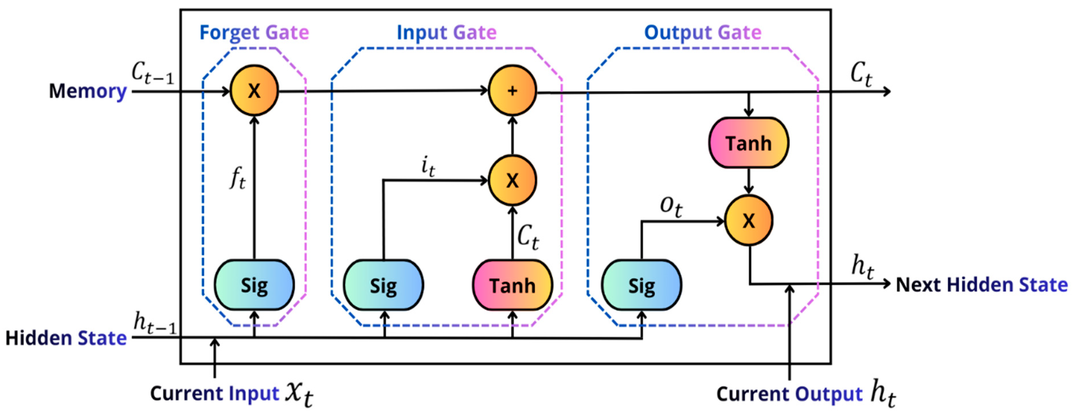
An LSTM unit is the basic component of an LSTM network and controls how information flows from one time step to the next. As shown in Figure 3, each unit includes a cell state with three gates: the input gate, the forget gate, and the output gate. The cell state serves as a memory pathway that preserves long-term information, while the gates regulate what to add, what to forget, and what to pass on to the next hidden state. Using sigmoid activations, these gates filter information between 0 and 1, allowing the LSTM to selectively remember or discard past data and reducing the vanishing gradient problem found in standard recurrent models.

More specifically, the input gate ($i_t$) controls the total information to be integrated from the present input of the sequence, as described in Equation (1). Similarly, the cell information (${\tilde{C}}_t$) is updated using the hyperbolic tangent activation function defined by Equation (2). The forget gate (f_t) fixes the amount of information to forget from the earlier state, as specified in Equation (3). The update gate ($C_t$) associates a fraction of the old cell information, updated by the input gate according to Equation (4), with the information unable to be remembered by the forget gate. Finally, the output gate ($O_t$) produces the new long-term memory ($C_t$) and computes the output of the present state ($h_t$), as expressed in Equations (5) and (6) [38].

$$i_t=\sigma \left(w_i\left[h_{t-1},x_t\right]+b_i\right)$$

(1)

$${\tilde{C}}_t=Tangh\left(w_C\left[h_{t-1},x_t\right]+b_C\right)$$

(2)

$$f_t=\sigma \left(w_f\left[h_{t-1},x_t\right]+b_f\right)$$

(3)

$$C_t=f_t{C}_{t-1}+i_t\cdot {\tilde{C}}_t$$

(4)

$$O_t=\sigma \left(w_O\left[h_{t-1},x_t\right]+b_O\right)$$

(5)

$$h_t=O_{t}Tangh\left(c_t\right)$$

(6)

Recent research has proposed several architectural variants of the LSTM network to enhance its ability to model complex temporal dependencies in time-series data. While an LSTM network uses a single recurrent layer of LSTM cells in one (forward) time direction, modern applications often employ deeper or more complex topologies to better model temporal dynamics. The Bidirectional LSTM (BiLSTM) extends the conventional unidirectional LSTM by processing input sequences in both forward and backward directions, thereby capturing contextual information from both past and future time steps within a given window. This bidirectional structure enables the network to utilize both past and future contextual information and it has been shown to improve forecasting accuracy in domains such as financial and energy load prediction, where temporal dependencies are not strictly causal [39,40]. The Stacked LSTM, on the other hand, consists of multiple LSTM layers stacked hierarchically, allowing the model to learn representations at different temporal scales. Deeper LSTM structures have demonstrated superior performance in capturing both short- and long-term dynamics in complex sequences [41,42]. More recently, the Stacked Bidirectional LSTM (Stacked BiLSTM) integrates both depth and bidirectionality by stacking multiple BiLSTM layers, enabling the extraction of high-level, bidirectional temporal features. This architecture has been successfully applied in short-term load and traffic forecasting, achieving enhanced predictive accuracy compared to single-layer or unidirectional models [40,42]. Collectively, these LSTM variants provide flexible and powerful frameworks for time-series forecasting, offering varying trade-offs between modeling complexity, interpretability, and computational efficiency.

Overall, the aforementioned LSTM variants, namely the Bidirectional LSTM (BiLSTM), Stacked LSTM, and Stacked Bidirectional LSTM (Stacked BiLSTM), have been widely recommended in the literature for their ability to capture complex temporal dynamics in time-series forecasting tasks [39,42]. Each variant offers distinct advantages: BiLSTM effectively leverages bidirectional temporal dependencies, Stacked LSTM enhances feature abstraction through deeper layers, and Stacked BiLSTM combines both mechanisms to achieve richer temporal representations. However, no single configuration consistently outperforms others across all datasets and forecasting horizons, as performance often depends on the specific characteristics of the time series, such as nonlinearity, periodicity, and noise level [43,44]. Therefore, to leverage the complementary strengths of these architectures and improve predictive robustness, we propose a novel combination of ensemble LSTM models. This ensemble framework integrates multiple LSTM-based learners, allowing their outputs to be adaptively combined to minimize generalization error and enhance forecasting accuracy. By fusing the predictive capabilities of different LSTM architectures, the proposed model aims to achieve superior performance and stability across diverse time-series forecasting scenarios.

In this paper, we propose to use four different methods to identify, each time, the accurate prediction between LSTM, BiLSTM, Stacked LSTM, and Stacked BiLSTM. These methods are summarized in

Table 5. Overview of the used benchmark methods for LSTM prediction evaluation and selection.

Method	Process	Rationale	Ref
Median or Trimmed Mean Rule	Take the median of the four predictions (or a trimmed mean if you want to exclude outliers).	The median is robust to extreme predictions and often performs well when no single model consistently dominates.	[45]
Instantaneous Model Selection via Minimized Consensus Error	✓ Compute the average of the four predictions. ✓ Select the model whose prediction is closest to the mean (or median).	The model closest to the consensus is likely the least biased for that instant.	[46]
Winner-Take-All by Minimal Deviation	At each time step, pick the prediction that minimizes a short-term error criterion based on a small recent window of actual values (if available).	This uses only the predictions and recent actuals to decide which model is currently most accurate.	[47]
Instantaneous Weighted Voting (Prediction Pooling)	Assign weights to the four predictions based on their relative agreement: If predictions are close, average them. If one prediction is an outlier, reduce its weight or discard it.	This creates a dynamic, “self-contained” ensemble based only on the predictions’ relative positions.	[48]

. To fully leverage the complementary strengths of different LSTM architectures, we implement an ensemble framework combining LSTM, BiLSTM, Stacked LSTM, and Stacked BiLSTM models. Individually, each architecture captures distinct temporal patterns: LSTM models long-term dependencies; BiLSTM incorporates both past and future context; Stacked LSTM extracts hierarchical features across multiple layers; and Stacked BiLSTM combines depth and bidirectionality for multi-scale temporal representations. By integrating these models, the ensemble adaptively selects the most reliable prediction at each time step, reducing the impact of inaccurate forecasts from any single model. This approach enhances predictive accuracy, stability, and robustness, making it particularly effective for complex and highly variable noisy time-series datasets. Table 5 summarizes four established methods used for evaluating and selecting LSTM model predictions. These benchmark methods serve as reference approaches for combining and/or selecting predictions from multiple models. While these methods are not part of the proposed framework, they provide a useful basis for comparison and highlight the advantages of our ensemble-LSTM approach. Specifically, the proposed ensemble-LSTM model leverages a GRU-based meta-learner to integrate complementary outputs from multiple LSTM architectures, offering improved robustness, predictive accuracy, and adaptability compared to conventional selection or aggregation techniques.

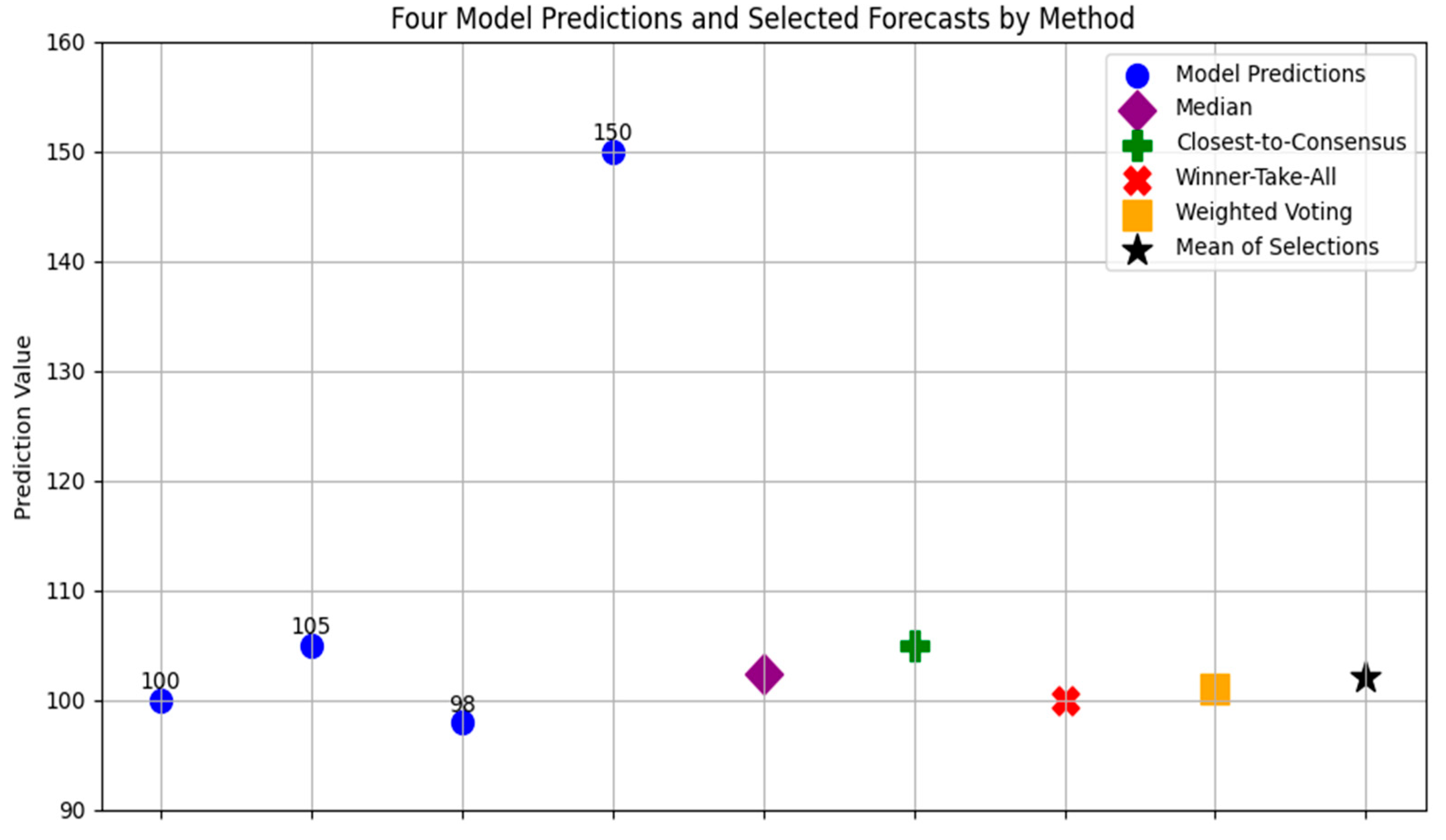
In situations where multiple forecasting models produce predictions for the same time instant, and no single model consistently outperforms the others, instantaneous prediction selection or aggregation methods presented in Table 5 can be applied using only the predicted values. Let us consider four models producing predictions y1(t), y2(t), y3(t), y4(t), at a given time step. A simple and robust approach is the median rule, which selects the median of the four predictions as the final forecast. For instance, if y1(t) = 100, y2(t) = 105, y3(t) = 98, y4(t) = 150, the median is 102.5, effectively mitigating the impact of the outlier (y4(t)). A related approach is the closest-to-consensus method, where the model whose prediction is nearest to the mean or median of the predictions is selected. Using the same example, the mean is (100 + 105 + 98 + 150)/4 = 113.25 and the prediction closest to the mean is y2(t) = 105. The winner-take-all strategy with short-term reference selects the model with minimal recent forecasting error; for example, if the last observed value was 102, the prediction closest to 102 is y1(t) = 100. Finally, the instantaneous weighted voting (prediction pooling) approach assigns dynamic weights based on the relative agreement among predictions. Predictions near the cluster center receive higher weight, while outliers are down-weighted. In our example, ignoring the outlier y4(t) = 150 and averaging the remaining three predictions gives a pooled forecast of (100 + 105 + 98)/3 ≈ 101. For better clarification and visualization, this numerical example is well illustrated in Figure 4. We propose, in this work, to use the mean of the previous four selections (median method result = 102.5, closest-to-mean result = 105, winner-take-all result = 100, and instantaneous weighted pooling result = 101) that is equal to 102.125. These methods have been widely discussed in the literature and provide a systematic way to improve forecast accuracy when multiple models are available without relying on historical performance or external meta-features [45,46,47,48]. In the next section, we will present and discuss the accuracy of the proposed ensemble-LSTM predictions’ selection strategy.

4. Experimental Results and Discussion

Experimental data were collected from a high-speed CNC machine under dry milling conditions using a three-flute ball nose tungsten carbide cutter on stainless steel (HRC 52). The cutting parameters were as follows: spindle speed 10,400 rpm, feed rate 1555 mm/min (X direction), radial depth of cut 0.125 mm (Y direction), and axial depth of cut 0.2 mm (Z direction). The PHM’2010 dataset was acquired at 50 kHz/channel. Despite that it consists of six individual cutters, the corresponding tool wear measurements are available only for three of them. Consequently, only these three cutter records, namely C1, C4, and C6, can be used to evaluate the proposed PHM approach. For each run, time-series sensor signals with lengths exceeding 200,000 time steps were recorded, resulting in a total of 315 runs per cutter. Such long sequences are adequate to evaluate predictive models.

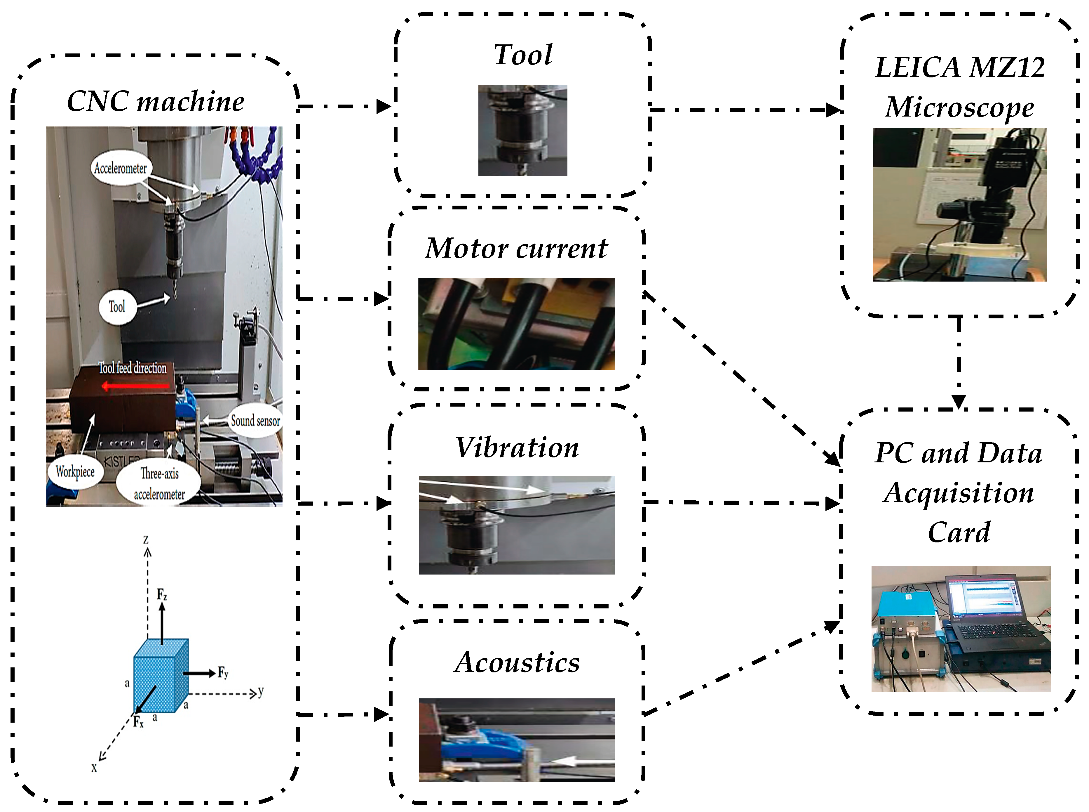
Considering the mechanical product process, each pass contains approximately 200,000 measurements from various sensors: cutting force components (Fx, Fy, Fz), vibration velocities (Vx, Vy, Vz), and the Acoustic Emission Root Mean Square (AERMS) signal. A total of 315 passes per cutter is realized. For each pass we compute the minimum, the average, and the maximum values, considering vibrations and the acoustic emissions. Hence, for each sensor measurement (Fx, Fy, Fz, Vx, Vy, Vz, AERMS), three statistical metrics are computed, considering that each milling cutter has three flutes and wear is recorded after every cut for each one. The cutter is deemed end-of-life when the wear on any single flute exceeds the specified limit. For this reason, the maximum wear among the three flutes is retained as the representative measure of tool degradation. 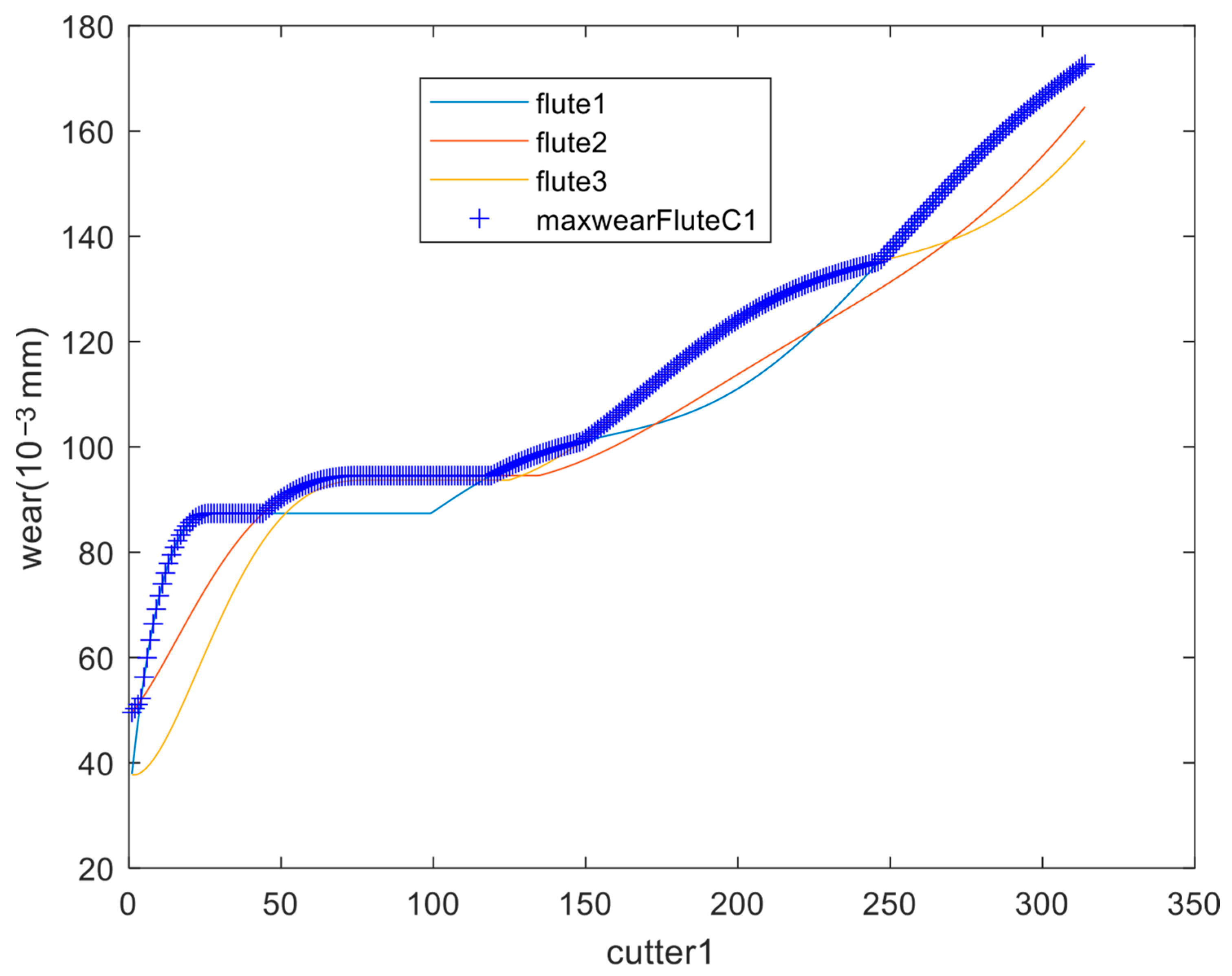Figure 5 shows the wear evolution of the cutter C1 in the three flutes and the maximum wear of them. The maximal accepted tool wear is 0.165 mm to standardize the condition monitoring of milling tools and to facilitate the development and evaluation of predictive models for tool wear and RUL. This threshold is intentionally set lower than the typical industrial standards that suggest for any CNC tool to be replaced when flank wear (VB) reaches approximately 0.3–0.6 mm.

In order to evaluate the prediction capabilities of the different proposed LSTM models, two scenarios are proposed in this paper based on cutter C6:

✓

Without data pre-processing original recoded data;

✓

With normalized data.

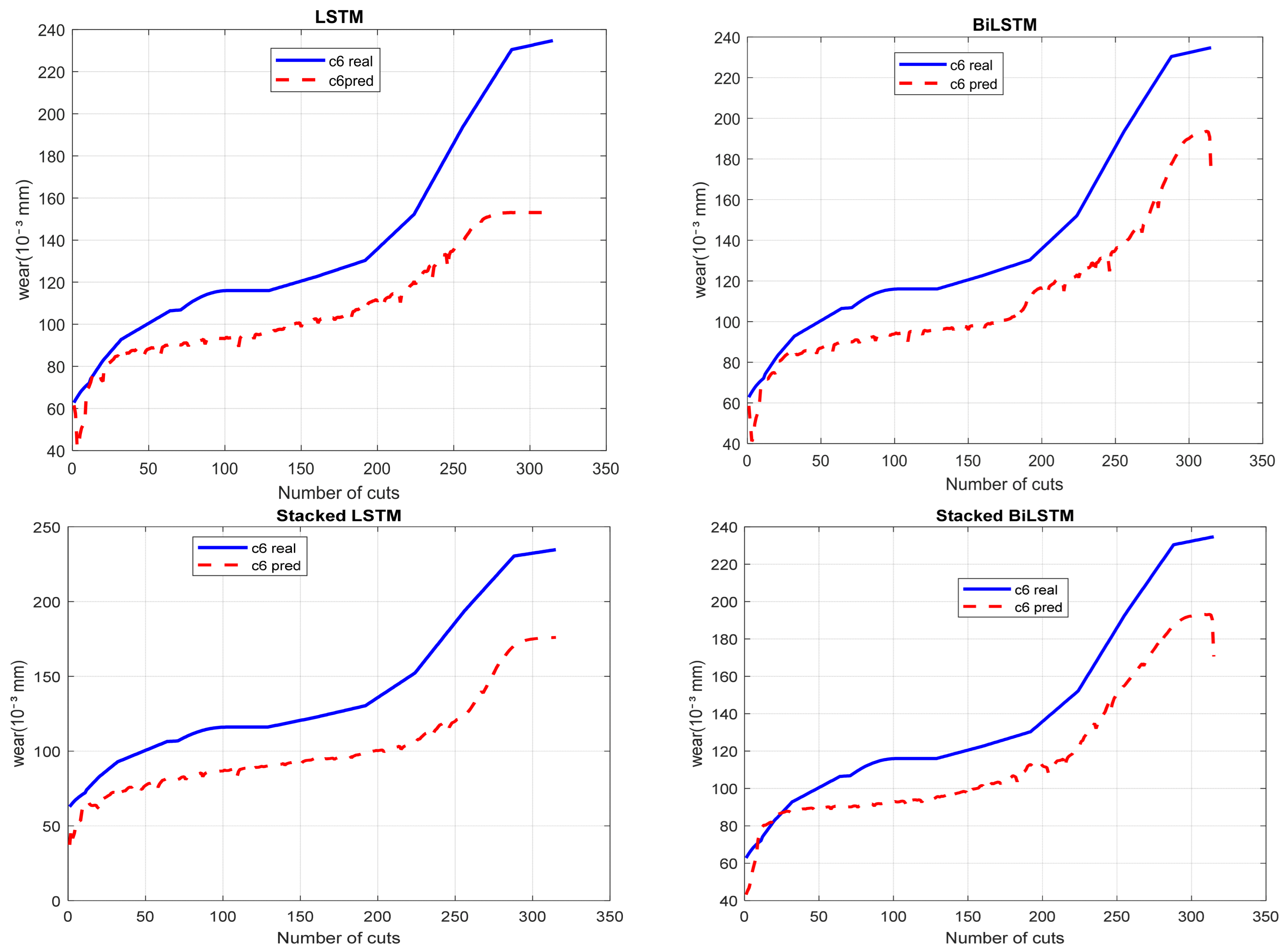
Figure 6 presents the prediction degradation results of milling tool wear using LSTM, BiLSTM, Stacked LSTM, and Stacked BiLSTM models. The cutters C1 and C4 are used for training the models using original recorder signals and the cutter C6 was used for testing. All models closely follow the trend of the real wear, demonstrating their capability to capture the tool degradation pattern, even if they do not fully converge to the exact measured values. In many previously published studies, an 80/20 random split of data from the same cutting tool run-to-failure history is commonly adopted, with 80% of the data used for training and the remaining 20% for testing. However, for time-series forecasting problems, such a strategy may introduce data leakage as degradation patterns from the same cutting tool can appear in both subsets. To provide a more realistic evaluation of model generalizability, a cutting-tool-level split (i.e., a leave-one-case-out assessment) was employed in this study. Specifically, the complete run-to-failure histories of cases C1 and C4 were used for model training, while the full run-to-failure history of case C6 was reserved exclusively for testing.

Graphical analysis reveals that the Stacked BiLSTM model delivers the best performance in both the overall curve trend and prediction accuracy. The Stacked LSTM model also demonstrates strong trend-capturing ability, closely following the actual data pattern but with slightly reduced accuracy compared to the Stacked BiLSTM. The BiLSTM model performs moderately well, while the standard LSTM exhibits the lowest accuracy among the tested models.

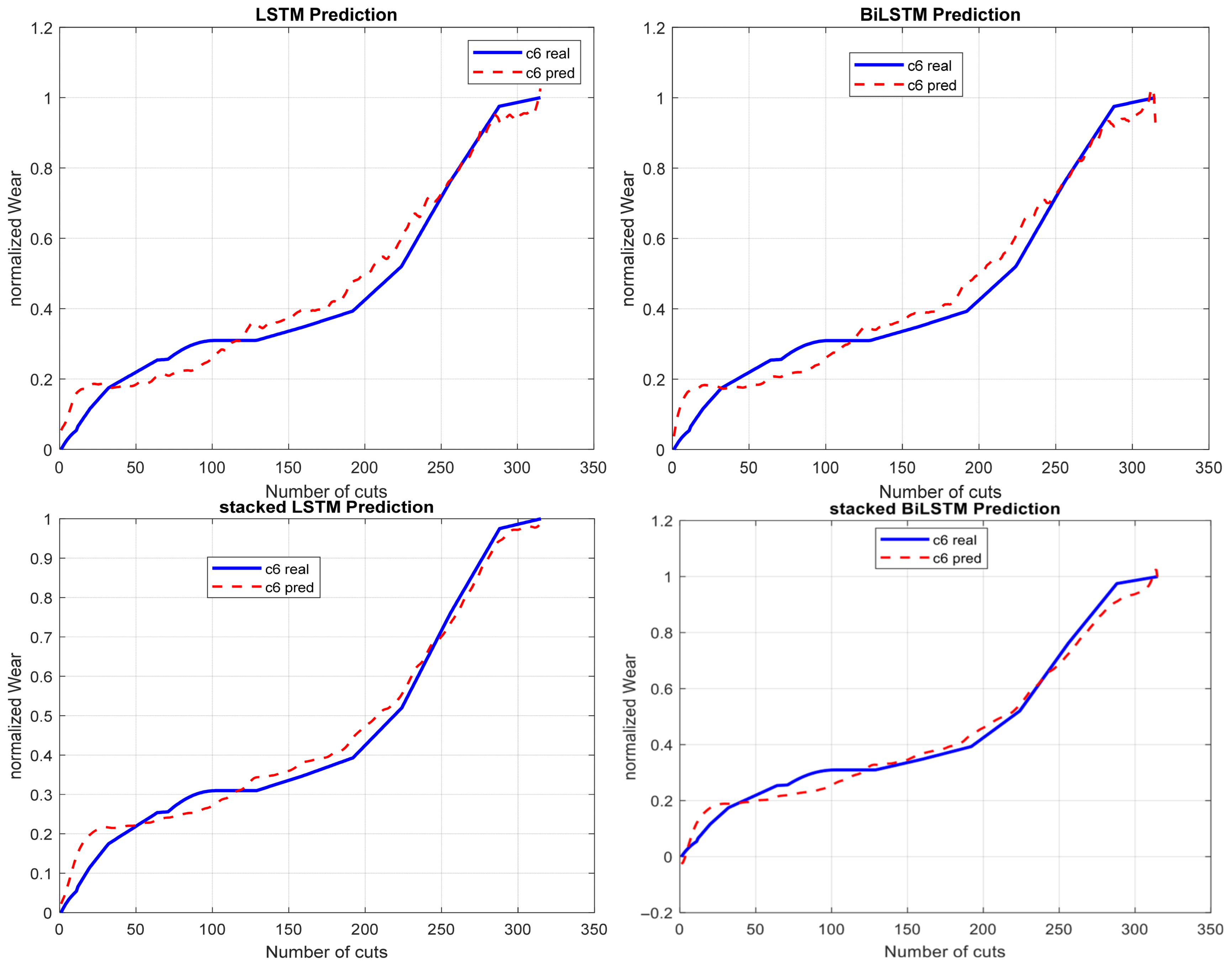
Training LSTM-based architectures on raw (unprocessed data) negatively affects model performance. Variations in the scales of input features (Fx, Fy, Fz, Vx, Vy, Vz, AERMS) and the presence of outliers can slow down the learning process, leading to unstable convergence. As a result, models trained on unprocessed data often exhibit slower convergence rates, limited generalization ability, and a higher risk of overfitting. These findings highlight the importance of data pre-processing, including normalization and outlier mitigation, to enhance the robustness and accuracy of deep learning models in time-series prediction tasks. Thereby, we propose to use the Hamming filtering before the computation of the normalized features (minimum, average, and the maximum) based on vibrations and acoustic emissions. Without normalization or standardization, the model underfits smaller-scale variables. This imbalance leads to slower convergence, reduced generalization, and an increased risk of overfitting. Conversely, applying pre-processing techniques such as min-max normalization and outlier removal improves feature consistency, resulting in faster training and more accurate predictions. As shown in Figure 7, experimental results indicate that pre-processing plays a crucial role in improving the quality and learnability of vibration and acoustic data. By normalizing feature scales, filtering noise, and removing outliers, pre-processing enhances the consistency and reliability of the input signals. These steps help LSTM models to converge more efficiently and produce more stable and accurate predictions. These steps guarantee that features with different physical units, such as forces (Fx, Fy, Fz), velocities (Vx, Vy, Vz), and acoustic emission energy (AERMS) contribute equally to the learning process. Additionally, Hamming filtering noises suppress irrelevant fluctuations while preserving critical features, improving signal-to-noise ratio and model generalization. Overall, pre-processing reduces computational complexity, minimizes the risk of overfitting, and enhances the interpretability of model outputs. As shown in Figure 7 and

Table 6. Evaluation of LSTM models.

	LSTM	BiLSTM	Stacked LSTM	Stacked BiLSTM
RMSE	0.0491	0.0506	0.0347	0.0353
MAE	0.0426	0.0435	0.0298	0.0307

, these pre-processing steps enhance the signal-to-noise ratio and contribute to a more robust and accurate predictive LSTM model.

Data pre-processing further enhances model robustness, emphasizing the importance of input standardization and outlier control in deep learning applications involving sequential data. Overall, the Stacked BiLSTM model demonstrates the most reliable and accurate performance for time-series prediction compared to other models. However, predictions for the same time instant show that Stacked BiLSTM predictions cannot outperform other models each time instant. For example, as shown in

Table 7. Instantaneous evaluation of LSTM models (cutting number 47 and 250).

Cutting Number	LSTM	BiLSTM	Stacked LSTM	Stacked BiLSTM	Real Measure
47	0.174	0.177	0.221	0.191	0.214
250	0.687	0.7	0.663	0.697	0.724

, Stacked outperforms other models at the cutting number 47 and BiLSTM outperforms other models at the cutting number 250. Thereby, instantaneous prediction selection or aggregation methods can be applied using only the predicted values.

More truthful results can be realized through the use of the proposed ensemble framework, which combines the result of each single model to enhance accuracy. The prediction result of the ensemble framework is usually superior to the prediction of a single model [49]. For this, we propose in this study a Gated Recurrent Unit (GRU)-based ensemble framework designed to enhance predictive accuracy by integrating the outputs of multiple LSTM-based models. 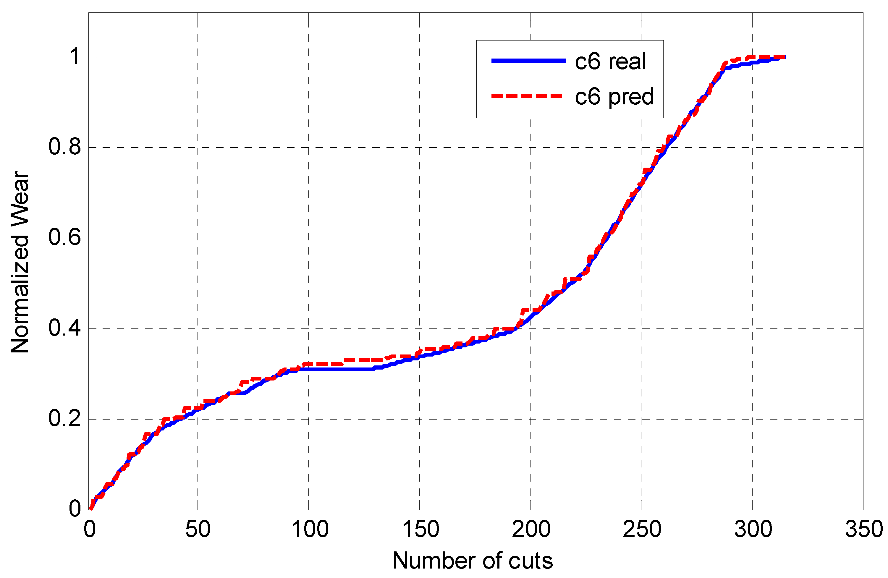Specifically, predictions generated by four distinct LSTM algorithms with the five selected forecasts (see Figure 4) are used as sequential input features to the GRU network, which functions as a meta-learner. The GRU architecture is particularly well-suited for this task due to its ability to capture temporal dependencies and nonlinear interactions among input signals while mitigating issues related to vanishing gradients. By learning complex dynamic relationships among the individual model predictions, the proposed GRU ensemble aims to produce a refined meta-prediction that more closely approximates the true target values than any single constituent model. When using a recurrent neural network such as a GRU for forecasting, the raw predictions may fluctuate due to noise or overfitting, sometimes producing a non-monotonic sequence. Hence, the GRU is adjusted by selecting the maximum value between two successive predictions. This is can be explicated physically by the monotonic behavior of the wear tool degradation. As shown in Figure 8 and

Table 8. Evaluation of the proposed ensemble-LSTM models’ combination.

	Ensemble-LSTM Models’ Combination
Normalized RMSE	0.0102
Normalized MAE	0.0085

, this approach leverages the complementary strengths and compensates for the weaknesses of the individual predictors, thereby achieving improved robustness, stability, and overall predictive performance.

The proposed ensemble-LSTM models’ combination exhibits notable superiority over conventional single-model and traditional ensemble forecasting approaches. By employing the GRU network as a meta-learner to integrate the predictions of multiple LSTM-based models, the framework effectively captures both nonlinear and temporal dependencies among the constituent predictors. This hierarchical learning structure allows the ensemble to exploit complementary features while mitigating the individual weaknesses of each base model, resulting in enhanced generalization capability and reduced predictive uncertainty. Moreover, the incorporation of a monotonic adjustment mechanism ensures that the final forecasts adhere to the physical characteristics of the tool wear process, thereby maintaining consistency with the underlying degradation dynamics. Comparative experimental analyses with some previous works (using the same dataset and the same C6 experiment for an expressive comparison) demonstrate that the proposed ensemble consistently achieves lower prediction errors, smoother degradation trajectories, and higher robustness against noise and outliers compared to the single LSTM predictive model. These results given in

Table 9. Proposed method performance comparison with some previous works based on the C6 PHM’2010 experiment.

Methods	RMSE	MAE
RNN [25]	32.9	25.5
1D-CNN [50]	15.748	13.002
Deep LSTMs [25]	18.9	15.2
LSTM [51]	21.2	14.6
HLLSTM [52]	8.8	7.1
TDConvLSTM [16]	10.22	7.50
ConvLSTM-Att [50]	5.716	4.056
CNN-LSTM [50]	10.646	7.749
Proposed method	2.4018	1.9969

confirm the efficacy and reliability of the proposed method as a superior predictive modeling approach for complex, temporally evolving systems.

Based on the experimental plan and results presented in this study, several important conclusions can be drawn from both the experimental evaluation and the predictive performance of the proposed framework. From an experimental perspective, the comparative analysis of individual LSTM-based architectures demonstrates that no single recurrent model is universally optimal under all machining conditions. Variations in cutting parameters, tool work-piece interactions, and sensor noise significantly affect model behavior, highlighting the necessity of systematic benchmarking under realistic industrial conditions. The tool wear behavior in CNC milling is highly nonlinear and sensitive to variations in cutting conditions, sensor noise, and operational dynamics. The experimental results confirm that deeper and bidirectional architectures improve temporal feature extraction but may suffer from overfitting or reduced robustness when operating conditions deviate from the training distribution. From a predictive standpoint, the ensemble-LSTM framework consistently delivers superior accuracy and stability by integrating complementary temporal representations through a GRU-based meta-learner. This predictive improvement is particularly evident in its ability to track progressive tool wear trends and maintain reliable RUL estimates under unseen operating scenarios, which is critical for deployment in real-world CNC machining environments.

Despite these promising results, several open challenges remain for CNC cutting tool RUL prediction in the context of Industry 4.0 (automation and digitalization of factories (IoT, Big Data) for efficiency and competitiveness) and the emerging paradigm of Industry 5.0 (human-centered dimension, promoting human–machine collaboration (cobots) for sustainable mass personalization, while integrating resilience and environmental and social sustainability). Modern smart manufacturing systems are characterized by highly heterogeneous data sources, including multi-modal sensor streams, cyber–physical systems, digital twins, and human-in-the-loop decision-making. Accurately modeling tool degradation in such environments requires not only higher predictive accuracy but also improved model interpretability, adaptability, and real-time responsiveness. Furthermore, frequent changes in machining tasks, materials, and tool geometries introduce domain shifts that challenge the generalization capability of data-driven models. Future work should therefore focus on incorporating transfer learning, online learning, and domain adaptation techniques to enable continuous model updating without costly retraining. In addition, integrating physics-informed constraints, uncertainty quantification, and explainable Artificial Intelligence (AI) mechanisms will be essential to enhance trustworthiness and decision support for human operators, aligning with the human-centric goals of Industry 5.0. Ultimately, addressing these challenges will enable the development of intelligent, resilient, and scalable PHM systems capable of supporting autonomous and collaborative CNC machining operations in next-generation smart factories.

5. Conclusions

Effective PHM of cutting tools in CNC milling machines is essential for minimizing downtime, improving product quality, and reducing maintenance costs in smart manufacturing environments. This study makes two main contributions. First, a comprehensive comparative evaluation of four LSTM-based architectures was conducted using real industrial CNC machining data under variable loads and dynamic operating conditions. This analysis clarified the strengths and weaknesses of each architecture and highlighted their sensitivity to operating variations, providing actionable insights for model selection in practical scenarios. Second, a novel ensemble-LSTM framework was developed to integrate multiple LSTM architectures using a GRU-based meta-learner. This approach effectively leverages complementary model strengths, resulting in improved robustness, generalization, and predictive performance. Quantitatively, the ensemble-LSTM achieved an RMSE of 2.4018 and an MAE of 1.9969, outperforming individual LSTM models across all test cases. Qualitatively, the model accurately tracks progressive tool wear trends and adapts to unseen machining conditions, demonstrating strong resilience to sensor noise and process variability. For future work, we propose the investigation of physics-informed constraints, uncertainty quantification, and explainable AI methods to enhance model interpretability, reliability, and decision support for human operators, in line with the human-centric objectives of Industry 5.0.