Evaluation of Regression Models for Predicting Cutting Forces Based on Spindle Speed, Feed Speed and Milling Strategy During MDF Board Milling

Abstract

This study investigates the influence of selected technical and technological parameters on cutting forces and power consumption during the milling of medium-density fibreboards. Unlike previous studies that focus primarily on force measurement, this work integrates experimental analysis with machine learning-based predictive modelling to improve process understanding and prediction accuracy. The main objective was to experimentally measure orthogonal cutting force components (F_x, F_y, F_z) and electrical power consumption under varying spindle speeds (14,000, 16,000 and 18,000 rpm), feed speed (6, 8 and 10 m/min), and milling strategies (conventional and climb), and to evaluate the suitability of the obtained data for predictive modelling. Cutting forces were measured using a Kistler 9257B piezoelectric dynamometer, and power consumption was recorded by a three-phase power quality analyser. Statistical analysis confirmed significant effects of machining parameters on force components, total cutting force, and power consumption. Spindle speed showed the strongest influence on total cutting force and power consumption, while milling strategy predominantly affected F_x and F_y components. Power consumption increased with increasing spindle speed. Based on the measured data, several machine learning models were developed to predict the total cutting force. The Fine Tree algorithm demonstrated the best performance, achieving validation metrics of R² = 0.9 and RMSE = 0.60 (MSE = 0.36, MAE = 0.48), and improved testing performance with R² = 0.95 and RMSE = 0.44 (MSE = 0.20, MAE = 0.36). After model comparison using RMSE, R², training time, and model size, a Fine Tree model was identified as the most suitable, achieving high prediction accuracy without signs of overfitting. The results confirm that experimentally obtained data on cutting force and electrical energy consumption are suitable for reliable predictive modelling in CNC milling of MDF boards. However, it is necessary to work with those components that have the greatest dependence on speed, feed, or type of milling, and these are the force components measured on the x and y axes.

1. Introduction

In modern manufacturing, cutting parameters play a vital role in the milling process and have a significant effect on tools and workpieces. As such, it is paramount to consider cutting forces and their effect during the milling process for several reasons, such as tool wear, surface quality, dimensional accuracy, machine stability and energy consumption as mentioned Petre and Găvrus [1], Chatterjee et al. [2], and Hernández-González et al. [3]. Wyeth et al. [4], Anh and Tung [5], and Felhő et al. [6] proposed that considering cutting forces and their effects during milling can help optimize the machining parameters in the manufacturing process.

Despite extensive research on cutting force modelling, several limitations can be identified in the existing literature. Experimental and analytical studies by Petre and Găvrus [1] and Anh and Tung [5] primarily focus on the relationship between machining parameters and cutting forces, often without integrating energy consumption analysis.

Milling is one of the most widely used manufacturing processes, yet accurate understanding of power consumption and cutting forces under milling conditions remains not utilized to its full potential. As power consumption is directly related to energy efficiency and the operational cost manufacturing sector, it requires reliable data and reasons to improve the milling process. Experimental investigations reported by Korkmaz et al. [7] show considerable variability in measured cutting forces and power consumption, particularly with respect to the influence of cutting speed, feed rate, depth of cut and type of materials. Franz [8] described that effect of cutting speed on cutting forces can have no impact. Contradictorily Pahlitzsch and Dziobek [9] and Porankiewicz et al. [10] described an increasing impact of cutting speed on cutting forces. Hlásková et al. [11] and Orlowski and Ochrymiuk [12] described that an increase in feed per tooth corresponds to an increase in chip thickness, which results in greater cutting forces and power consumption. Overall differences in machine tools, measurement systems, and cutting conditions make it difficult to simply compare results or generalize conclusions. Based on this there is a need for measurement of cutting forces and power consumption during the process of milling. Data are required not only to better understand the process of milling but also to validate predictive models and support overall optimization of processes aimed at energy consumption without decreasing quality of milling performance.

Creating a low-cost, constrained-motion dynamometer for milling applications is difficult. Gomez and Schmitz [13] proposed that some designs achieve accurate three-axis force measurement at a fraction of the cost of commercial systems, addressing the need for more affordable and adaptable measurement tools in research and industry.

Luo et al. [14] used a milling table integrated with PVDF thin-film sensors to measure cutting forces without an external dynamometer. This research demonstrated a lightweight, flexible approach to force sensing, showing the evolution toward embedded and intelligent measurement systems in milling operations. Cutting force measurement has a critical role in understanding machining performance, tool wear, and surface quality. Rosca et al. [15] used accurate force data from a dynamometer to analyse tool condition and optimize process parameters in difficult-to-cut materials.

Wood and other types of boards can be created from recycled wood or lower quality wood materials. Wood as a material is plentiful, renewable and resourceful; it is a material that is used in furniture manufacturing. By focusing research on milling wood-based agglomerates we can expand our current knowledge of new types of materials, their energy efficiency and forces applied onto materials during the milling process. As the material is produced locally, it creates the opportunity in the future for expansion of products that would be modified using milling processes.

Dynamometers are the most reliable instruments for direct cutting force monitoring. Sousa et al. [16] mentioned that there are several types of dynamometers that use different sensing methods, such as piezoelectric, strain-gauge, and others. Dynamometers can measure four-component forces in real time. Yun et al. [17] confirmed that this design significantly improves sensitivity and response speed, representing a step forward in dynamic and multi-axis force measurement for high-speed milling. Bal and Dumanoğlu [18] demonstrated that energy consumption increases with higher spindle speeds and decreases with higher feed rates, while surface quality follows the opposite trend. Ji and Zhu [19] described that cutting parameters affect both cutting forces and cutting temperature during face milling of a material. Silva et al. [20] mentioned that milling strategies influence productivity, roughness and vibration; these are important parameters while searching for optimal milling paths.

Reported prediction performance in the literature varies depending on the applied method and dataset, with typical values ranging from R² ≈ 0.80 to 0.93 and RMSE values often exceeding 0.50 in machining applications described by Chatterjee et al. [2], Hernández-González et al. [3], and Ji and Zhu [19]. In comparison, the model developed in this study achieved R² = 0.95 and RMSE = 0.44 on testing data, indicating improved predictive performance and strong generalisation capability. Furthermore, review studies by Korkmaz et al. [7] and Sousa et al. [16] highlight that many models do not simultaneously evaluate prediction accuracy and computational efficiency.

This article deals with the use of cutting force and cutting power data obtained during the milling of medium-density fibre wood boards to create predictive models using machine learning. The study’s conclusions expand current knowledge in the field of predictive modelling in the machining of wood-based agglomerates. First, the measured data are processed and evaluated statistically to determine the statistical significance of the effects of individual technical and technological milling parameters.

Following the statistical evaluation, machine learning models were created and parametrized. These models are then rigorously tested to assess their suitability for the specific type of data. The evaluation is based on the correlation coefficient of measured and predicted data, on their root main square error and on assessing the overfitting or underfitting of the model.

In contrast to previous studies, the present research combines high-precision experimental measurements of cutting force components with simultaneous monitoring of power consumption, providing a more comprehensive dataset for analysis. Additionally, multiple machine learning models are systematically developed and compared using both accuracy metrics (RMSE, R², MAE) and computational performance indicators (training time and model size), which are rarely considered together in existing studies. This integrated approach enables not only accurate prediction but also practical evaluation of model efficiency for industrial applications.

The main contribution of this research are:

• Experimental investigation of cutting force components (F_x, F_y, F_z) and electrical power consumption during CNC milling of MDF under varying machining conditions.
• Development and comparison of multiple machine learning models for predicting total cutting force.
• Quantitative evaluation of model performance using RMSE, R², MAE, as well as computational metrics such as training time and model size.
• Identification of an optimal predictive model (Fine Tree) achieving high accuracy (R² = 0.95, RMSE = 0.44) and efficient performance.

2. Materials and Methods

Samples of medium-density fibre (MDF) boards were used as the experimental material, which were cut to dimensions of 350 mm × 160 mm × 18 mm. Medium-density fibreboard (MDF) is an engineered wood product produced by hot-pressing wood fibres bound with synthetic resins, most commonly urea–formaldehyde (UF), under controlled heat and pressure as mentioned by Hong et al. [21]. The manufacturer of sample material MDF E1 (EN ISO 12460-5) [22], the company KRONOSPAN (Zvolen, Slovakia), guarantees technical specifications according to the technical sheet of the manufactured product. Material density is 750 kg·m³ ± 7%, and tolerance of thickness is ±0.2 mm. All other details are in the technical sheet on the manufacturer’s website. Before experimental measurement occurred, the material was formatted to the required dimensions and milled around the perimeter for the purpose of removal of unwanted shortcomings or inaccuracies.

2.1. Cutting Tool Used in Experiment

The tool used in the experiment was a spiral monolithic 3-spiral end mill SCH3UFN284R 20 × 90 × 20 (Freud, S.p.A, Pavia di Udine, Italy), with parameters in

Table 1. Parameters of cutting tool.

Parameter	Description/Value
Tool type	End mill
Construction	Monolithic (solid tool)
Cutting edge geometry	Spiral/Helical
Number of flutes	3
Tool diameter	20 mm
Chip removal	Positive

.

2.2. CNC Machining Centre

Measurements occurred using a 5-axis CNC machining centre, specifically a Z5-31 SCM TECH (SCM Group, Rimini, Italy). This CNC machine is well-suited for furniture panel production, designed for high-precision tasks in complex 3D shaping, contouring, and drilling operations. At the core of the machine is an 11 kW “Prisma 5” vertical electro-spindle with a high-speed capacity of up to 24,000 rpm, allowing it to handle demanding routing and milling operations. The spindle is belt-driven and water-cooled, ensuring consistent thermal management. The CNC machine spindle follows the HSK 63 standard [23], offering excellent rigidity and fast tool changes.

According to manufacturer [24] The CNC machine’s capability is supported by a broad movement envelope, typically around 3110 mm (X), 1300–1550 mm (Y), and 160 mm (Z), with continuous rotation along axes B (±320°) and C (±640°). This enables complex multi-sided machining without repositioning the workpiece. Safety and ergonomics are embedded into the machine design through features like bumper-style collision protection, automatic lubrication, and dust extraction interfaces. The control system is PC-based.

2.3. Power Consumption Mesurement

The device used for measurement of power consumption of the milling process was an MI 2893 Power Master XT (Metrel d.o.o., Horjul, Slovenia) three-phase power quality analyser, which complies with IEC 61000-4-30 [25] Class A and IEC 61557-12 [26] Class 1 standards. Based on the manufacturer specifications, voltage measurements have an accuracy of approximately ±0.1% of nominal voltage, and active power measurements are expected to have an uncertainty within ±1% of the reading under typical conditions The power analyser was connected to the electrical supply of the CNC machining centre using current probes and voltage clamps. The voltage clamps were attached to the phase conductors, as well as to the neutral and protective conductors, through the installed 32 A 5P socket. The current probes were positioned according to the direction of current flow; if connected in the opposite direction, the measured values at the terminals would appear as negative. After completing the measurement setup, a test measurement of the signal was performed on all phases.

The signal is sampled as 1024 data per cycle at 50/60 Hz frequency. All channels are sampled simultaneously. Power data storage is implemented at 1 s intervals. The program used for measuring power consumption was Metrel PowerView v3.0.

2.4. Cutting Forces Mesurement

Cutting force measurements were performed using a three-component piezoelectric dynamometer (Kistler 9257B, Kistler Group, Winterthur, Switzerland). The Kistler 9257B is a piezoelectric, multicomponent dynamometer designed to capture orthogonal force components F_x, F_y, F_z during machining operations, including milling, turning, and grinding. In our case we will be using it in the process of milling [27]. The dynamometer was operated with a ±100 N range, resulting in a measurement uncertainty of approximately ±1% of full-scale output (±1 N). This corresponds to a relative error of 1–5% depending on the measured force magnitude.

It integrates four three-component quartz force sensors, preload-mounted between a baseplate and a 100 × 170 mm top plate. This assembly enables measurement of forces and moments with high stiffness and natural frequency as is described by manufacturer [27].

The dynamometer was mounted onto wooden particleboard, which was fixed to the CNC machine centre using pneumatic grippers. This method was used for fixing the dynamometer in place during milling. The experimental sample was fastened onto the dynamometer with hex bolts that kept the material during the milling process fixed in place. We set minimal safe distance to be 50 millimetres. This area was monitored and marked. Tool path was closely monitored, and if the tool encroached onto the marked area the milling process would be stopped immediately.

The program used for cutting forces measurements was DynoWare v3.2.5.0. Sampling rate of signal during measurement was 5000 Hz. The entire milling cycle with one sample was recorded in one measurement, which includes 3 conventional and 3 climb millings. Overall force was computed as

$$F_c=\sqrt{F_x^2+F_y^2+F_z^2}$$

(1)

where F_x, F_y and F_z are measured forces in x, y and z axis according to the coordinate system of the dynamometer. Signal filtering was set to low pass with an edge frequency of 100 Hz and filter order n 64 using DynoWare software Version 3.3.2.0 for data analysis.

2.5. Cutting Parameters

The cutting parameters were selected according to the practical operation based on several factors of the CNC milling machine and the recommended cutting conditions for the applied cutting tool. Spindle speeds of 14,000, 16,000, and 18,000 rpm and feed speeds of 6, 8, and 10 m/min were chosen to cover a range of machining conditions commonly used in high-speed milling. These parameters are summarised in

Table 2. Parameters of variation used in experiment.

Parameter	Values
Spindle speed (rpm)	14,000, 16,000, 18,000
Tool feed rate (m/min)	6, 8, 10
Milling type	Conventional, Climb

. This range enabled the investigation of the influence of cutting speed and feed speed on the milling process while maintaining process stability and preventing excessive tool wear. Furthermore, both up milling (conventional milling) and down milling (climb milling) were employed to assess changes in power consumption and measurements of cutting forces. Figure 1 and Figure 2 show simplified drawings of the experiment’s dynamometer and material placed onto the pneumatic system of the CNC machine. There are 4 sensors inside the dynamometer that measure forces in directions F_x, F_y and F_z. The tool path is along axis Y with 3 passes on right side and with 3 passes on the left side; each pass removes a 1 mm layer of material.

The experiment was conducted using a Factorial Design, where spindle speed, tool feed rate, and milling type were selected as input factors. Experimental runs were performed using combinations of these parameters. The experiment consisted of 6 total passes of the milling tool, 3 conventional and 3 climb per sample. Depth of cut is equal to thickness of sample, which is 18 mm. The width of the removed layer was 2 mm. During the milling process on a CNC milling machine, the power consumption of milling and the cutting forces applied onto milled material were measured. The data collected by the measuring device were used to analyse the influence of machining parameters.

2.6. Other Factors

Measurement uncertainty is always a factor to consider, as such devices were calibrated and tested before the experiment occurred. A measuring device for force measurements is mounted onto the CNC machine using pneumatic grippers of the CNC centre. These pneumatic grippers can keep the board holding measuring device with sample in place without risk of movement due to pressure between the CNC and board with measuring device. During the experiment, multiple pneumatic grippers hold the board with measuring device in place. Measured forces will not exceed forces that could force pneumatic locks to fail.

Experiments were conducted in sequential order, which may introduce minor systematic bias. Tool wear was not explicitly considered in this study, as a new cutting tool was used throughout the experiments to maintain consistent conditions. However, tool wear may influence cutting forces and should be included in future studies to improve model generalisability.

3. Results

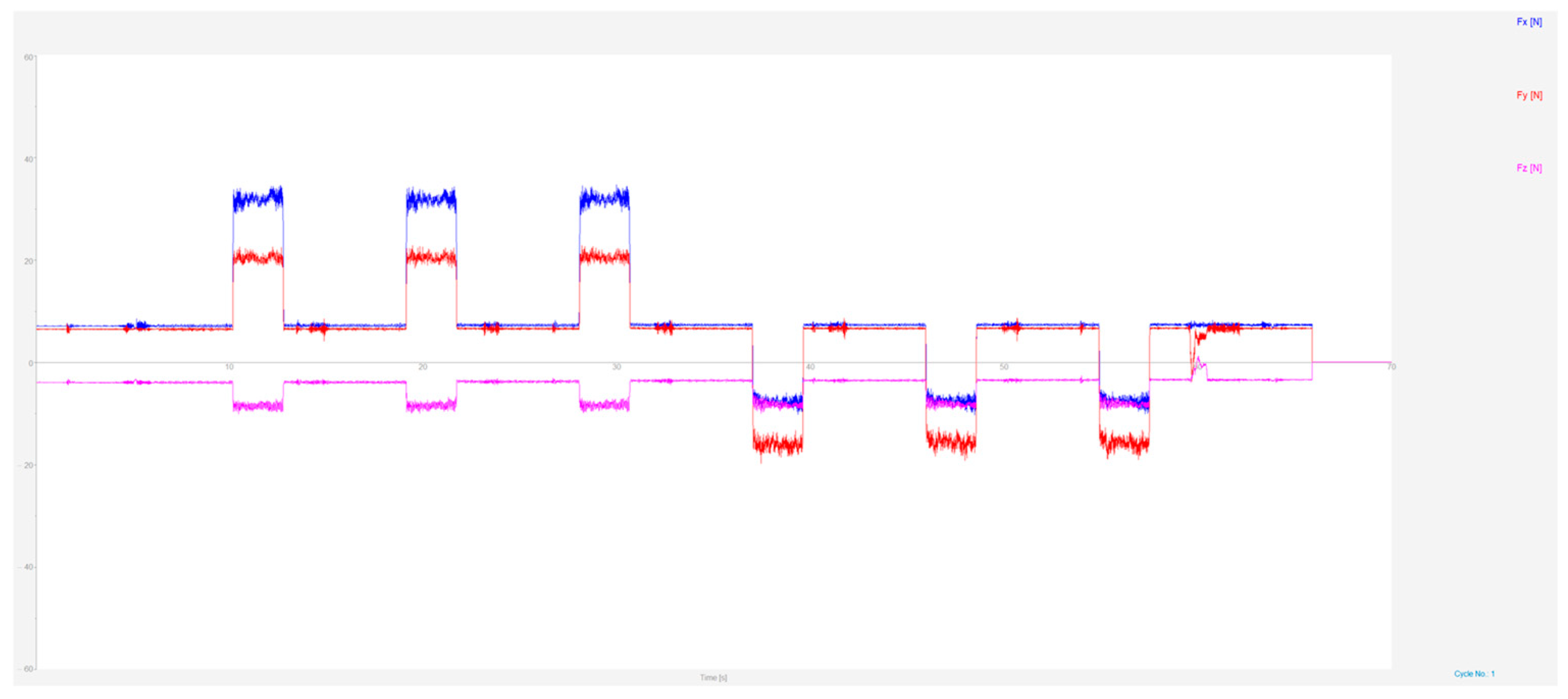
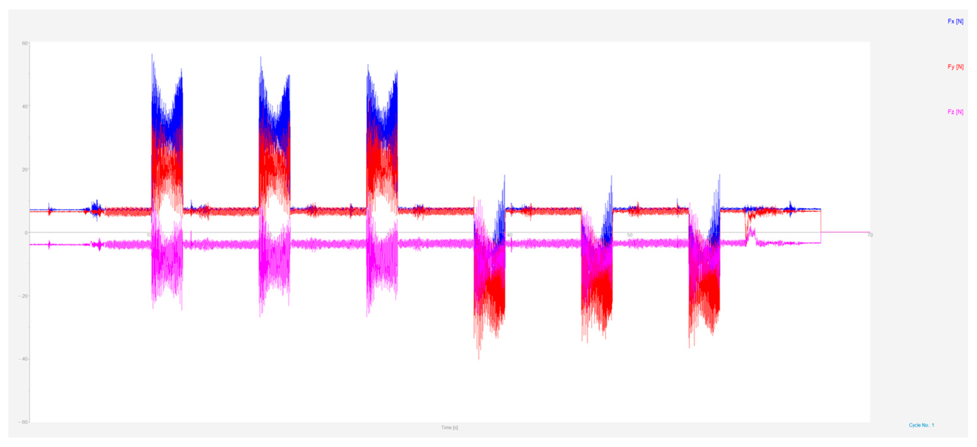
Power consumption was calculated as power consumed during milling process, from which was subtracted power consumption while the CNC machine was in idle mode. Cutting forces were more straightforward as the measuring tool has its own software that showed the entire experimental process with detailed graphs of any components of cutting forces. To work with data, random noise and volatility were reduced. This was done to reveal a clearer, more coherent signal for data analysis. All calculations were made by software, baring the exception of making it an absolute value, as depending on which side forces were applied one was negative. A negative value only meant that forces were applied in the other direction.

Figure 3 shows recorded data after three climb and three conventional millings. Figure 4 shows recorded data after filtering in DynoWare software by low pass filter with a lower edge frequency (−3 dB) of 20 Hz. Based on this figure, forces were calculated as the absolute value of difference between cutting force during idle time and cutting force during milling process. After the last milling pass (time 60 s) there is a slight change in forces; this was due to part of the CNC machine passing over and transferring forces with a rubber curtain.

3.1. Statistical Evaluation

The statistical significance of machining parameters was evaluated using analysis of variance (ANOVA), a method originally developed by Fisher [28] and widely applied in engineering experimental designs like Montgomery [29] to determine the relative contribution of cutting parameters to response variables.

For purpose of statistical evaluation, we used the program STATISTICA version 14.0.0.15 (TIBCO Software Inc., Palo Alto, CA, USA). This program was chosen based on availability, technical understanding of software, utilities and personal preference.

Table 3. Descriptive statistics of F_x.

Effect		Valid N	Mean	Std. Dev.	Std. Err	−95%	95%
Total		180	20.018	4.903	0.365	19.296	20.739
n (rpm)	14,000	60	20.423	5.166	0.667	19.089	21.758
	16,000	60	20.627	4.684	0.605	19.417	21.837
	18,000	60	19.003	4.767	0.615	17.771	20.234
f (m/min)	6	60	19.989	4.199	0.542	18.904	21.074
	8	60	20.158	4.884	0.631	18.896	21.420
	10	60	19.906	5.605	0.724	18.458	21.354
Climb		90	24.788	1.143	0.120	24.549	25.028
Conventional		90	15.247	1.009	0.106	15.035	15.458

,

Table 4. Descriptive statistics of F_y.

Effect		Valid N	Mean	Std. Dev.	Std. Err	−95%	95%
Total		180	19.382	5.088	0.379	18.633	20.130
n (rpm)	14,000	60	20.681	5.046	0.651	19.377	21.984
	16,000	60	19.801	5.192	0.670	18.460	21.143
	18,000	60	17.663	4.608	0.595	16.473	18.853
f (m/min)	6	60	17.628	5.184	0.669	16.289	18.967
	8	60	19.356	4.693	0.606	18.143	20.568
	10	60	21.162	4.827	0.623	19.915	22.409
Climb		90	14.727	2.074	0.219	14.292	15.161
Conventional		90	24.037	1.985	0.209	23.621	24.453

,

Table 5. Descriptive statistics of F_z.

Effect		Valid N	Mean	Std. Dev.	Std. Err	−95%	95%
Total		180	4.915	0.700	0.052	4.812	5.018
n (rpm)	14,000	60	5.512	0.499	0.064	5.383	5.641
	16,000	60	4.757	0.663	0.086	4.586	4.928
	18,000	60	4.476	0.464	0.060	4.357	4.596
f (m/min)	6	60	4.834	0.688	0.089	4.657	5.012
	8	60	4.778	0.595	0.077	4.624	4.932
	10	60	5.133	0.765	0.099	4.935	5.330
Climb		90	4.830	0.752	0.079	4.672	4.987
Conventional		90	5.000	0.636	0.067	4.867	5.134

,

Table 6. Descriptive statistics of P.

Effect		Valid N	Mean	Std. Dev.	Std. Err	−95%	95%
Total		180	0.145	0.041	0.003	0.139	0.151
n (rpm)	14,000	60	0.125	0.023	0.003	0.119	0.132
	16,000	60	0.127	0.030	0.004	0.119	0.134
	18,000	60	0.182	0.038	0.005	0.172	0.192
f (m/min)	6	60	0.122	0.023	0.003	0.116	0.128
	8	60	0.144	0.046	0.006	0.132	0.156
	10	60	0.168	0.037	0.005	0.158	0.177
Climb		90	0.145	0.039	0.004	0.137	0.153
Conventional		90	0.145	0.043	0.005	0.136	0.154

and

Table 7. Descriptive statistics of overall force Fc.

Effect		Valid N	Mean	Std. Dev.	Std. Err	−95%	95%
Total		180	29.101	1.952	0.146	28.814	29.388
n (rpm)	14,000	60	30.409	1.432	0.185	30.039	30.779
	16,000	60	29.785	1.246	0.161	29.464	30.107
	18,000	60	27.109	1.307	0.169	26.771	27.446
f (m/min)	6	60	27.842	1.669	0.215	27.411	28.273
	8	60	29.124	1.040	0.134	28.855	29.393
	10	60	30.337	2.128	0.275	29.787	30.887
Climb		90	29.271	2.008	0.212	28.850	29.691
Conventional		90	28.931	1.891	0.199	28.535	29.327

summarise descriptive statistics of measured variables. The main tool chosen for analysis was ANOVA (analysis of variance), in order to determine statistically significant differences between the means of independent groups for forces F_x, F_y, F_z, overall force F_c, and cutting power P. It is essential for comparing multiple groups simultaneously. For analysis purposes, we took all force components as absolute values, as during the experiment different combinations of feed speed (f), rotation of milling tool (n) and different types of milling (conventional, climb) were used.

Analysis of variance was conducted to examine the groups of data and if there are significant corelations. The Kolmogorov–Smirnov test of normality revealed that measured data are normally distributed and suitable for ANOVA.

Table 8. Analysis of variance.

Variable	SS	df	MS	SS	df	MS	F	p
P	0.250	17	0.0147	0.048	162	0.0003	49.259	<0.001
Fx	4276.886	17	251.582	26.703	162	0.1648	1526.290	<0.001
Fy	4607.697	17	271.041	26.497	162	0.1636	1657.138	<0.001
Fz	79.995	17	4.706	7.728	162	0.0477	98.640	<0.001
Fc	633.681	17	37.275	48.615	162	0.3000	124.212	<0.001

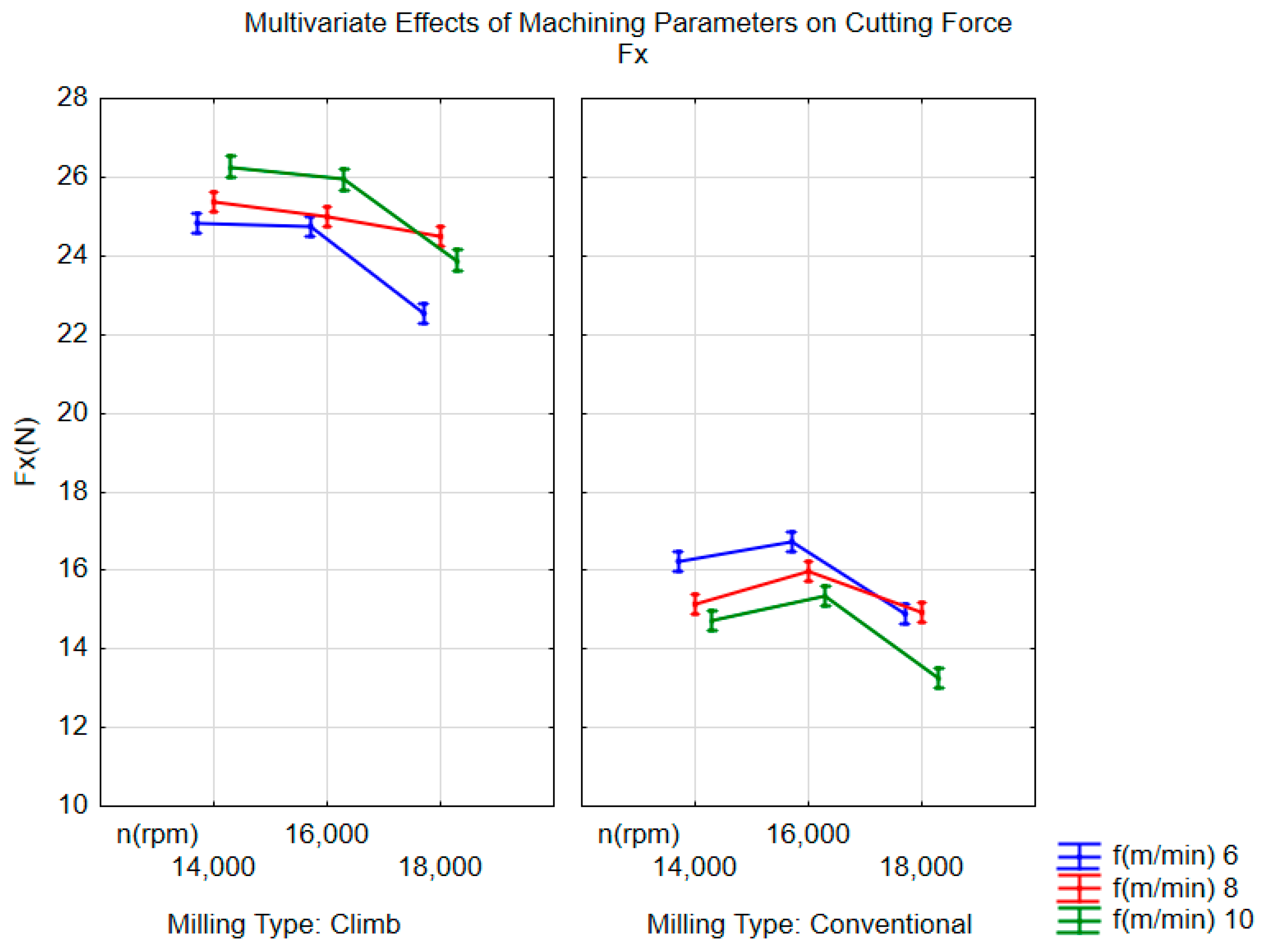
shows comparisons between the data acquired during the experiment. The highest influence of technological parameters was on the measured force F_x.

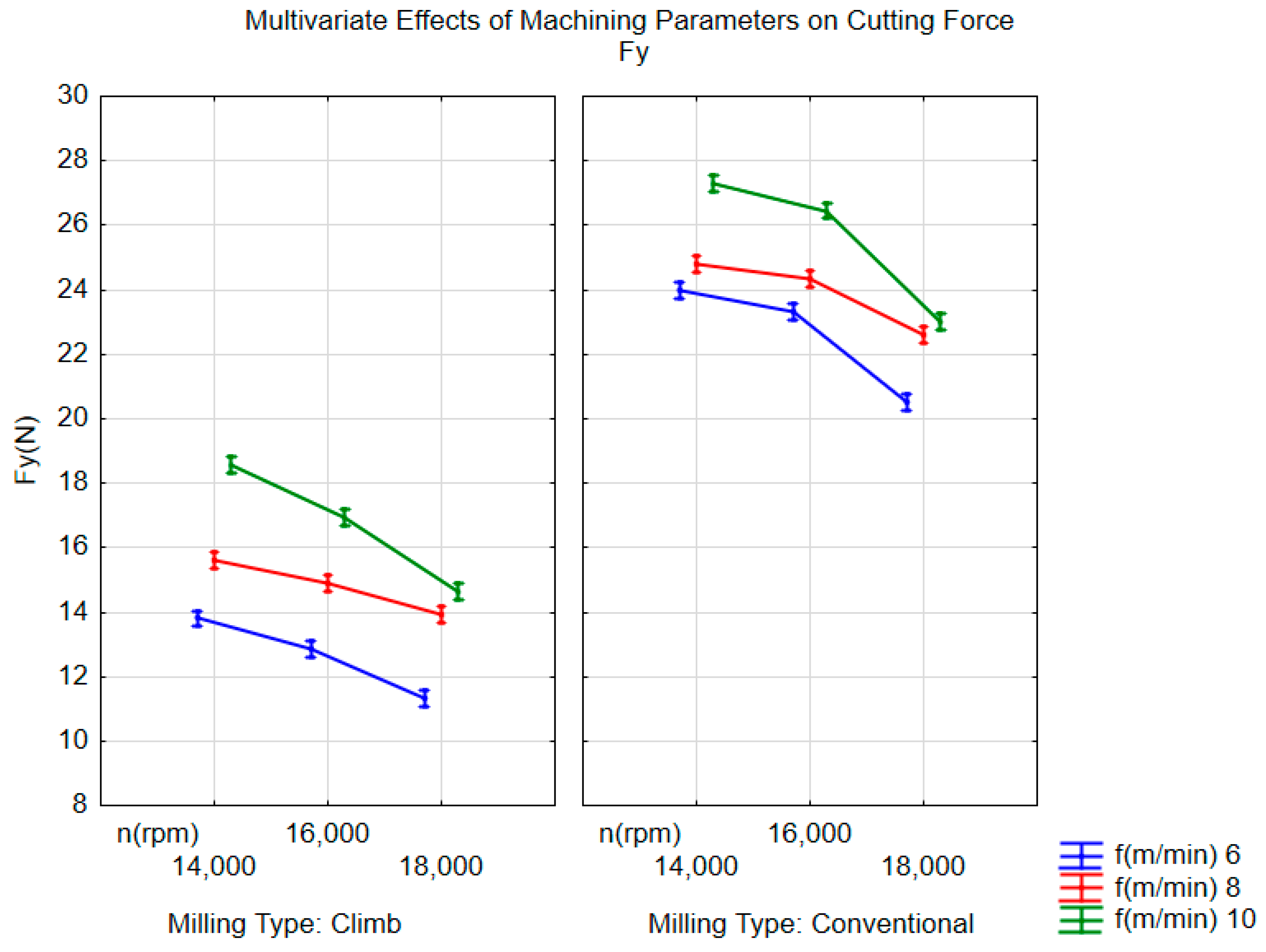
Figure 5 shows how the change of force F_x is influenced by milling parameters. Climb milling had a component of this force greater than conventional. According to Duncan’s test, the influence of individual independent observed factors on this force component is statistically significant (probability of similarity p < 0.05), except for the values at the feed speed of 6 and 10 m/min⁻¹ Figure 6 shows that with increase of feed speed, measured force F_y increases; also, the force decreases with increased revolutions of the cutting tool. Here, on the contrary, climb milling had a smaller component of this force than conventional milling. Duncan’s test showed a statistically significant effect (p < 0.05) of independent technological parameters on this force component. 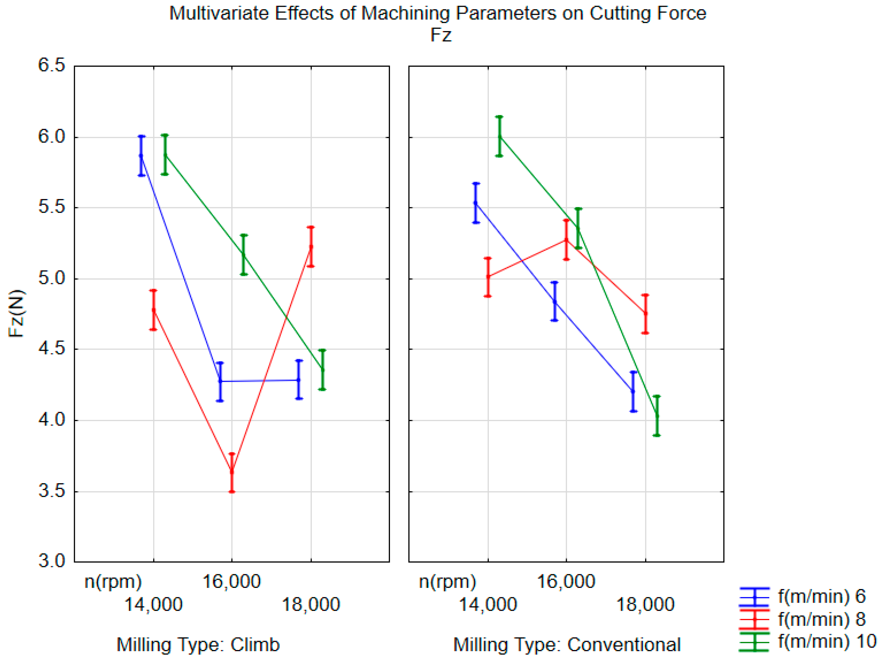Figure 7 shows how cutting parameters influence cutting force in direction F_z; the graph shows all cutting parameters are in range of each other with little change less than 2 N. According to Duncan’s test, the influence of individual independent observed factors on this force component is statistically significant (p < 0.05), except for the values at the feed speed of 6 and 8 m/min. All presented dependencies are related to the theory of wood composites milling, with individual components oriented according to the coordinate system of the force sensor. Their size is also influenced by the shape of the cutting edge of the tool and the change in the cross-section of the removed layer of material according to the type of milling. In terms of cutting energy specifically, the results can also be influenced by the material moisture and temperature. These were constant (8% and 22 °C) and standard for the selected machining conditions. The influence of vibrations was minimized by applying a low filter to the measured signal.

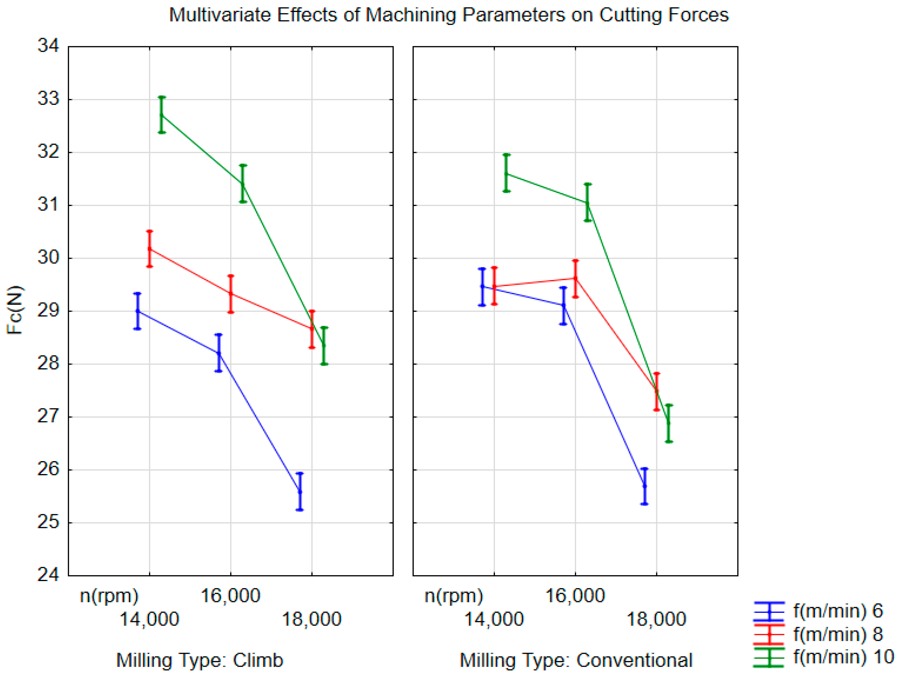
Figure 8 shows the dependence of computed force F_c on technological parameters. Computed force increases with increase of feed speed and decreases with increase of rotation of tool. This fact is also true for theory of cutting, when cutting force decreases with increase in cutting speed due to decreasing thickness of removed material. This dependency shows that force does not change much with change of milling type, although Duncan’s test also showed a statistically significant effect of individual factors on this force.

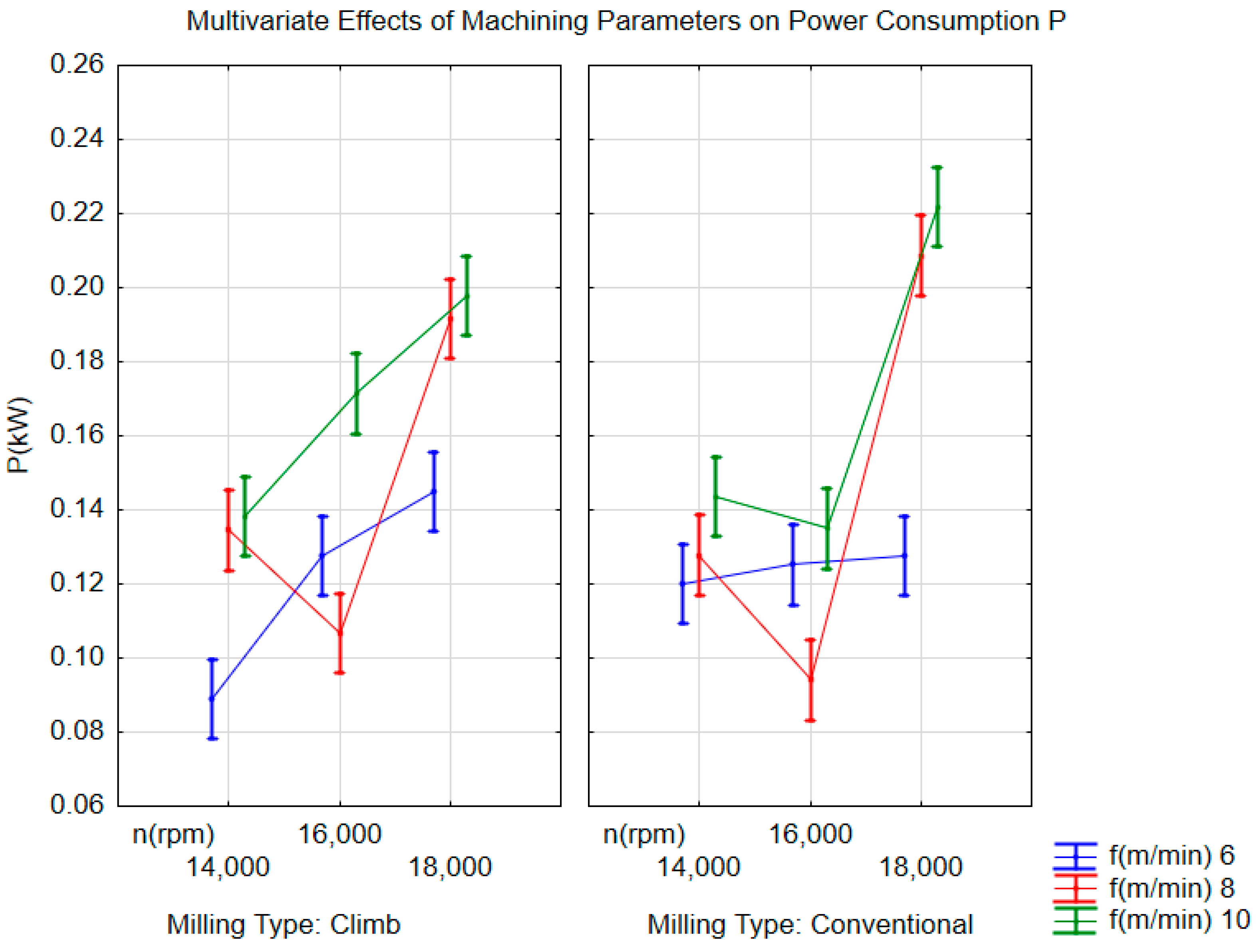
Figure 9 shows the dependence of the consumed power required for material removal by the technological parameters of milling. With increasing speed of rotation of the tool, the consumed electrical power increases mainly due to higher currents flowing through the electrical winding of the electric spindle.

F-test determines whether differences between group means are statistically significant by comparing variability between groups to variability within groups. In ANOVA, SS (Sum of Squares) measures total variation, MS (Mean Square) is SS divided by its degrees of freedom, F is the ratio of between-group variance to within-group variance (MS between/MS within), and p is the probability of observing such an F value if there is actually no real difference between groups.

In the F-test in

Table 9. F-test for parameter F_x.

Effect	SS	MS	F	p
n (rpm)	93.95	46.97	284.98	<0.001
f (m/min)	1.98	0.99	6.00	0.003
Milling Type	4096.73	4096.73	24,853.98	<0.001

,

Table 10. F-test for parameter F_y.

Effect	SS	MS	F	p
n (rpm)	289.00	144.50	883.48	<0.001
f (m/min)	374.74	187.37	1145.58	<0.001
Milling Type	3900.61	3900.61	23,848.25	<0.001

,

Table 11. F-test for parameter F_z.

Effect	SS	MS	F	p
n (rpm)	34.43	17.22	360.90	<0.001
f (m/min)	4.36	2.18	45.66	<0.001
Milling Type	1.31	1.31	27.38	<0.001

,

Table 12. F-test for parameter F_c.

Effect	SS	MS	F	p
n (rpm)	368.85	184.43	614.56	<0.001
f (m/min)	186.85	93.43	311.32	<0.001
Milling Type	5.19	5.19	17.31	<0.001

and

Table 13. F-test for parameter P.

Effect	SS	MS	F	p
n (rpm)	0.13	0.06	210.13	<0.001
f (m/min)	0.06	0.03	104.58	<0.001
Milling Type	0.00	0.00	0.01	0.931

, we can clearly see what parameters are statistically significant. Parameters that influence parameters are in red font.

From the data in Table 9, all examined factors have a statistically significant effect on the force F_x. Spindle speed n (rpm) demonstrates a strong influence (F = 284.98, p < 0.001), while feed rate f (m/min) also shows statistical significance (F = 6.00, p = 0.003). Milling type exhibits the highest F value (F = 24,853.98, p < 0.001), indicating that it is the dominant factor affecting F_x. Based on the magnitude of the F statistics, milling type contributes most substantially to variations in Fy, followed by spindle speed, whereas feed rate has a comparatively smaller effect.

All investigated factors are highly statistically significant (p < 0.001) for force F_y according to results in Table 10. Milling type yields the largest F value (F = 23,848.25), indicating the strongest influence on F_y. Feed rate (F = 1145.58) and spindle speed (F = 883.48) also demonstrate pronounced and statistically significant effects. These results confirm that Fz is strongly dependent on both cutting conditions and the selected milling type.

The F-test results in Table 11 reveal statistically significant effects of all three factors (p ≤ 0.001) for parameters F_z. Spindle speed shows the greatest impact (F = 360.90), followed by feed rate (F = 45.66). Although milling type is statistically significant (F = 27.38, p = 0.000001), its effect is comparatively smaller. Therefore, Fz is predominantly influenced by spindle speed, with secondary contributions from feed rate and milling type.

In Table 12, results indicate that spindle speed (F = 614.56, p < 0.001), feed rate (F = 311.32, p < 0.001), and milling type (F = 17.31, p < 0.001) all significantly influence parameter Fc. Among these factors, spindle speed exhibits the strongest effect, followed by feed rate, while milling type contributes to a lesser extent. Therefore, Fc is predominantly governed by cutting conditions.

The F-test for power consumption in Table 13 indicates that spindle speed (F = 210.13, p < 0.001) and feed rate (F = 104.58, p < 0.001) significantly influence the response. In contrast, milling type does not exhibit a statistically significant effect (F = 0.01, p = 0.931). This suggests that parameter P is determined mainly by cutting conditions rather than by the type of milling process.

3.2. Predictive Modelling

Matlab (R2024b Update 5) Regression Learner was used as a tool for creation of predictive models. The main goal was to predict total force F_c. This program allows a wide selection of different model types, their training, and testing, and is then followed by comparison. Main parameters used for comparison are Root Mean Square Error (RMSE) and coefficient of determination R². The parameters of RMSE of created models should be as close as possible to a value of 0. It is also important to compare RMSE values for the training and testing datasets. If trained and tested data have large differences between each other, it may indicate that the model has memorised the training data and is therefore unsuited for new data.

Measured data were randomly separated into two groups: trained (80%) and tested (20%) data. Data used as predictors for model training were spindle speed (n), feed speed (f) and milling type. The dependent variable was total force created by the milling tool during the process of material removal from workpieces. To choose the right model, initial training and testing were carried out using all available models in the Matlab environment, after which models were subsequently compared. The testing data originated from measured datasets obtained during experiments; this data is about 20% from total measured data. Data were randomly selected from each combination of machining parameters for testing data. Bayesian optimization as optimizer and expected improvement per second as acquisition function for 30 iterations were used for model optimisation.

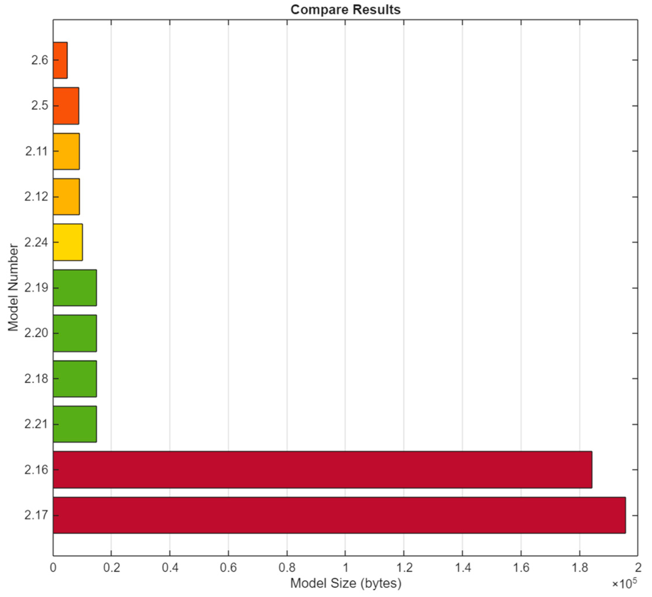
After filtering clearly unsuitable models (RMSE ≥ 0.7 and R² ≤ 0.8), the remaining models were further compared with respect to their size in bytes. The size of the resulting models for Boosted Trees (Model No. 2.16) and Bagged Trees (Model No. 2.17) exceeded 18 × 10⁴ bytes, while the other models were below 1.5 × 10⁴ bytes, as shown in Figure 10. With a larger dataset, this imbalance would be even more apparent, and for this reason models with this high requirement were removed from further analysis.

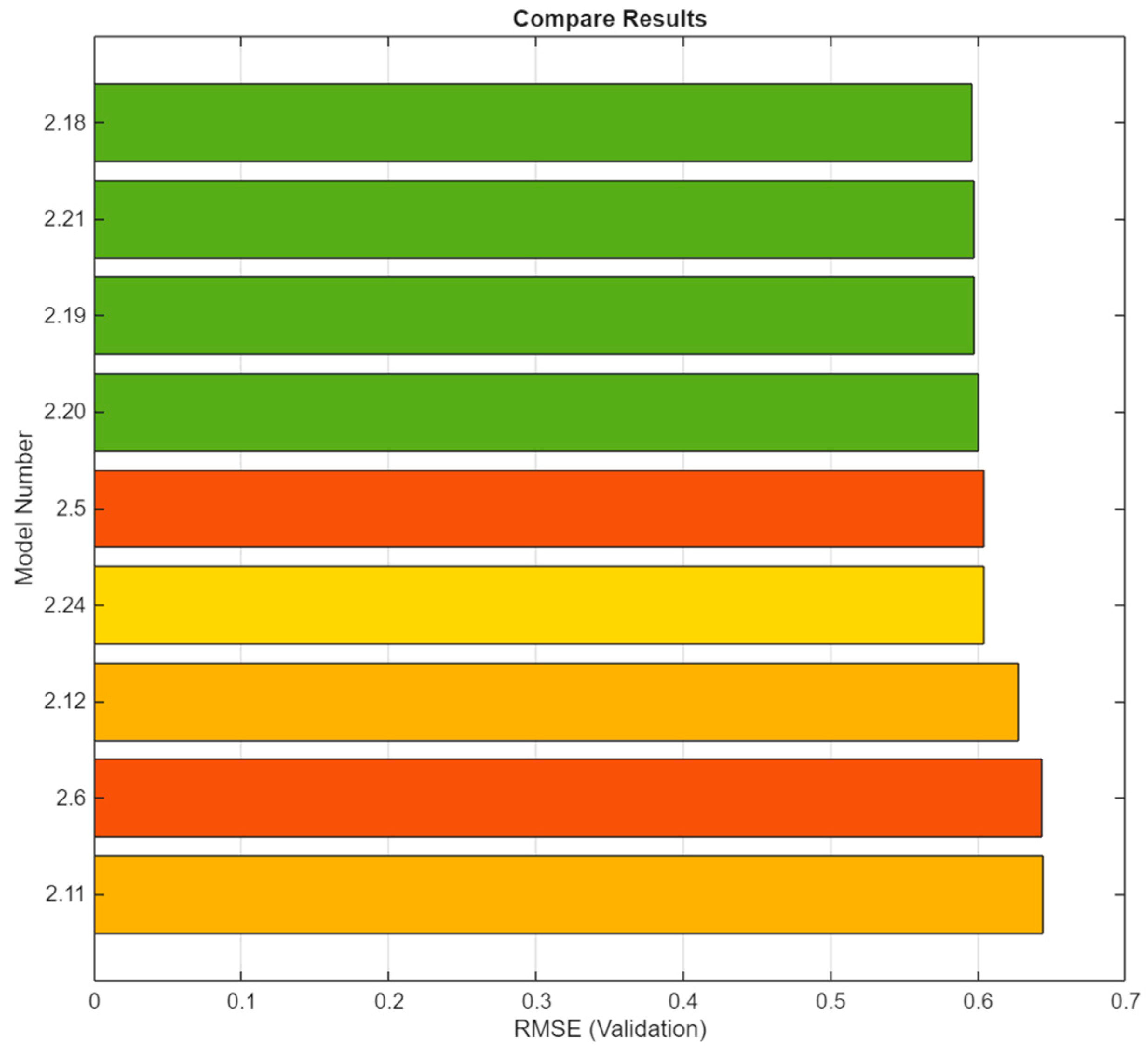
The filtered models (RMSE ≤ 0.7 and R² ≥ 0.8) are shown in Figure 11, with their RMSE and R² being very similar.

The values of RMSE (Root Mean Square Error), MSE (Mean Square Error), R² (Coefficient of determination) and MAE (Mean Absolute Error) for both validation and test are in

Table 14. Comparison of selected models.

Model Number	Model Type	Validated				Tested				Training Time (s)	Model Size (Bytes)
		RMSE	MSE	R2	MAE	MAE	MSE	RMSE	R2
2.18	Squared Exponential GPR	0.6	0.36	0.91	0.48	0.37	0.21	0.46	0.95	3.96	14,957
2.21	Rational Quadratic GPR	0.6	0.36	0.91	0.48	0.37	0.21	0.46	0.95	3.85	14,988
2.19	Matern 5/2 GPR	0.6	0.36	0.91	0.48	0.37	0.21	0.46	0.95	3.89	14,937
2.20	Exponential GPR	0.6	0.36	0.91	0.48	0.36	0.21	0.46	0.95	3.92	14,943
2.5	Fine Tree	0.6	0.36	0.9	0.48	0.36	0.2	0.44	0.95	3.88	8919
2.24	Wide Neural Network	0.6	0.37	0.9	0.49	0.36	0.2	0.44	0.95	4	10,117
2.12	Medium Gaussian SVM	0.63	0.39	0.9	0.51	0.38	0.26	0.51	0.93	3.47	9180
2.6	Medium Tree	0.64	0.41	0.89	0.51	0.52	0.41	0.64	0.9	3.88	4979
2.11	Fine Gaussian SVM	0.64	0.42	0.89	0.51	0.35	0.2	0.45	0.95	3.46	9100

. A 5-fold cross-validation method was used as a resampling technique for the model’s performance evaluation. The table also contains training time and model size. From their comparison, the Fine Tree model appears to be optimal, which has a low RMSE, short training time (3.88 s) and reasonable model size (8919 bytes).

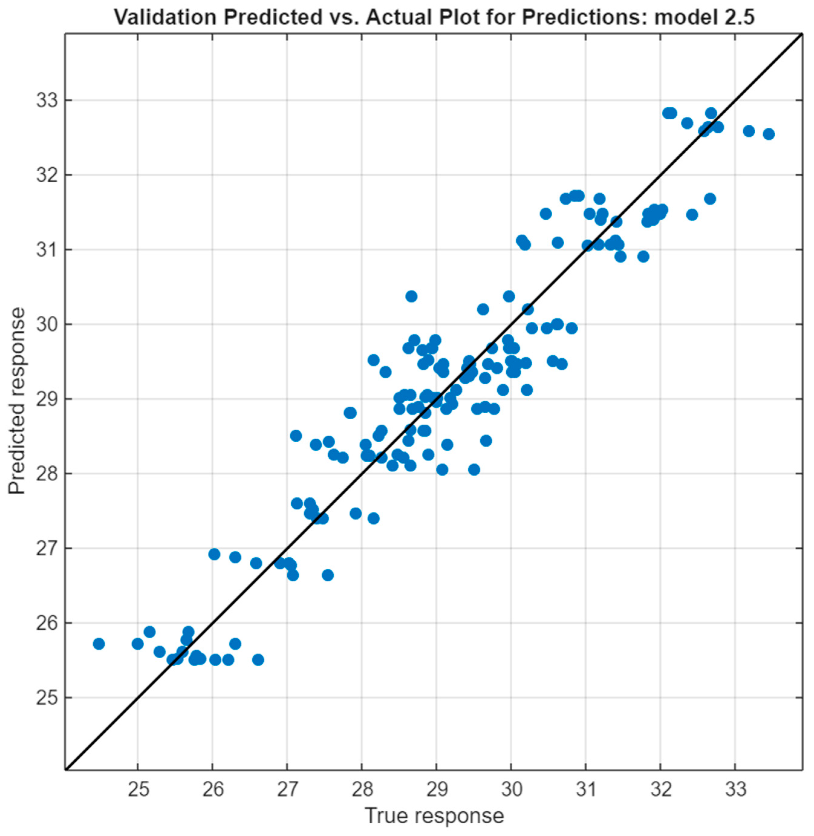
Based on the comparison in Table 14, the Fine Tree model (Model No. 2.5) was further analysed. Figure 12 shows the predicted response compared to the true response. These have an approximate linear relationship, where their distance from the black line represents the prediction model error. Fine Trees are variants of decision tree models, which belong to the class of non-linear models used in supervised learning.

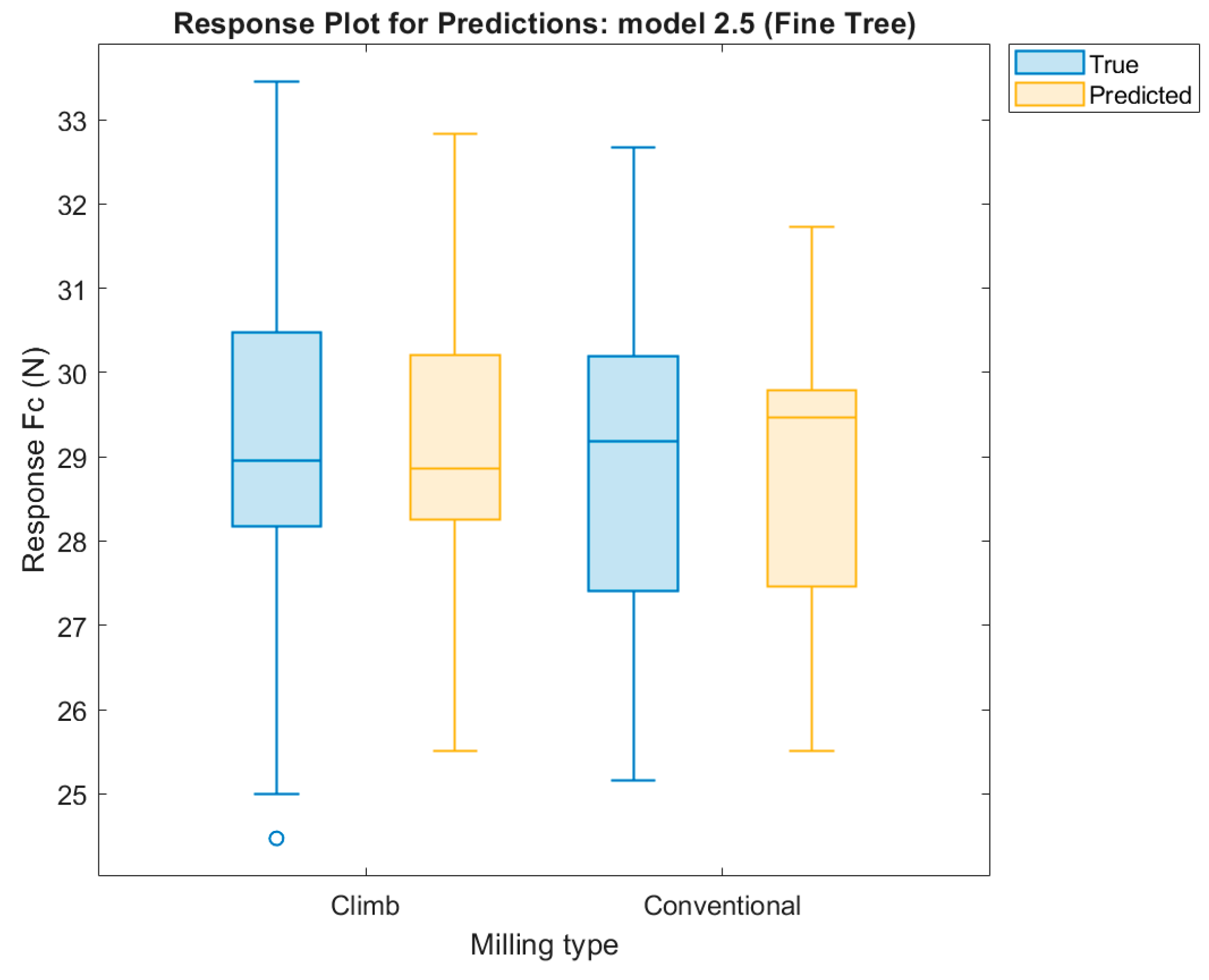
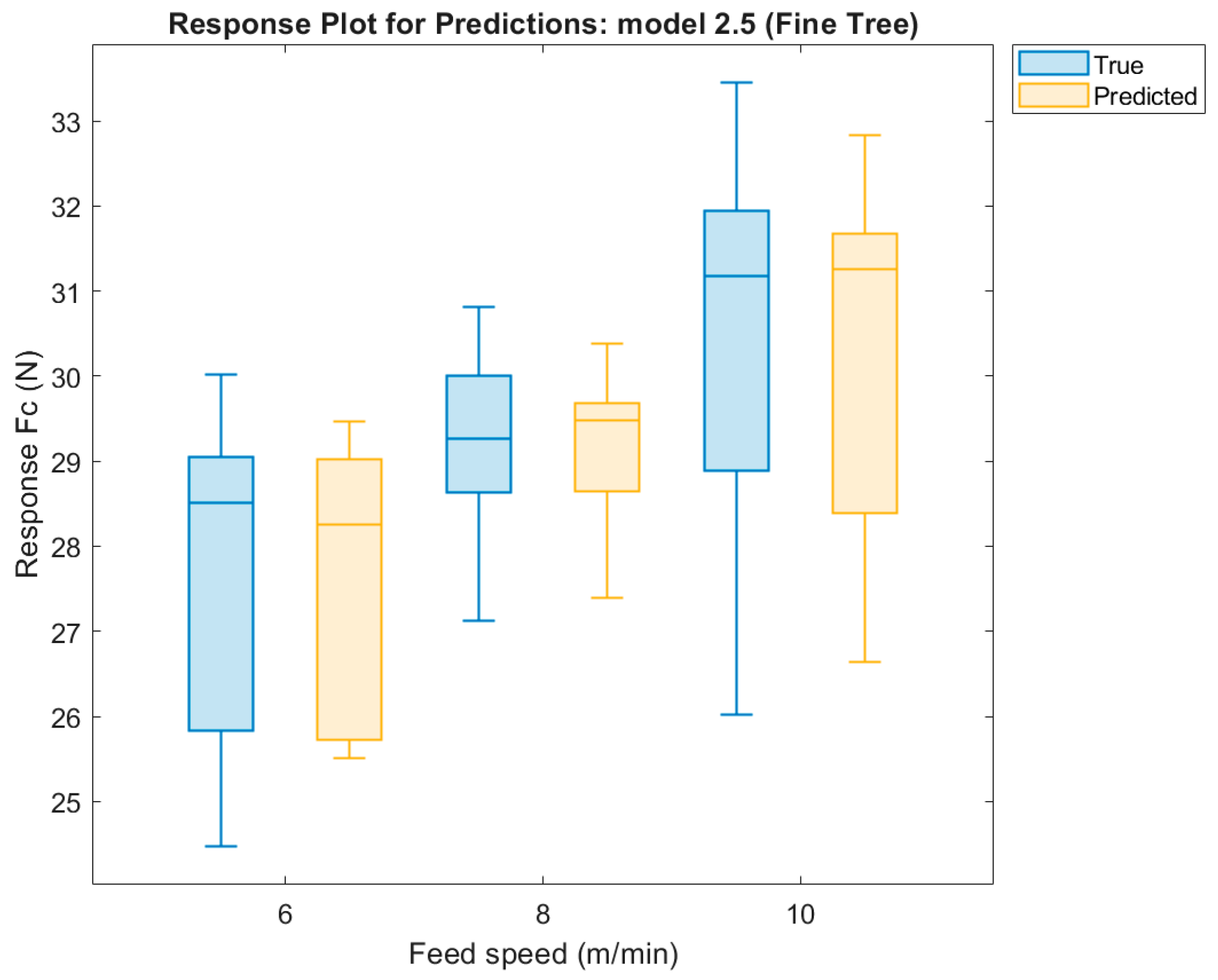
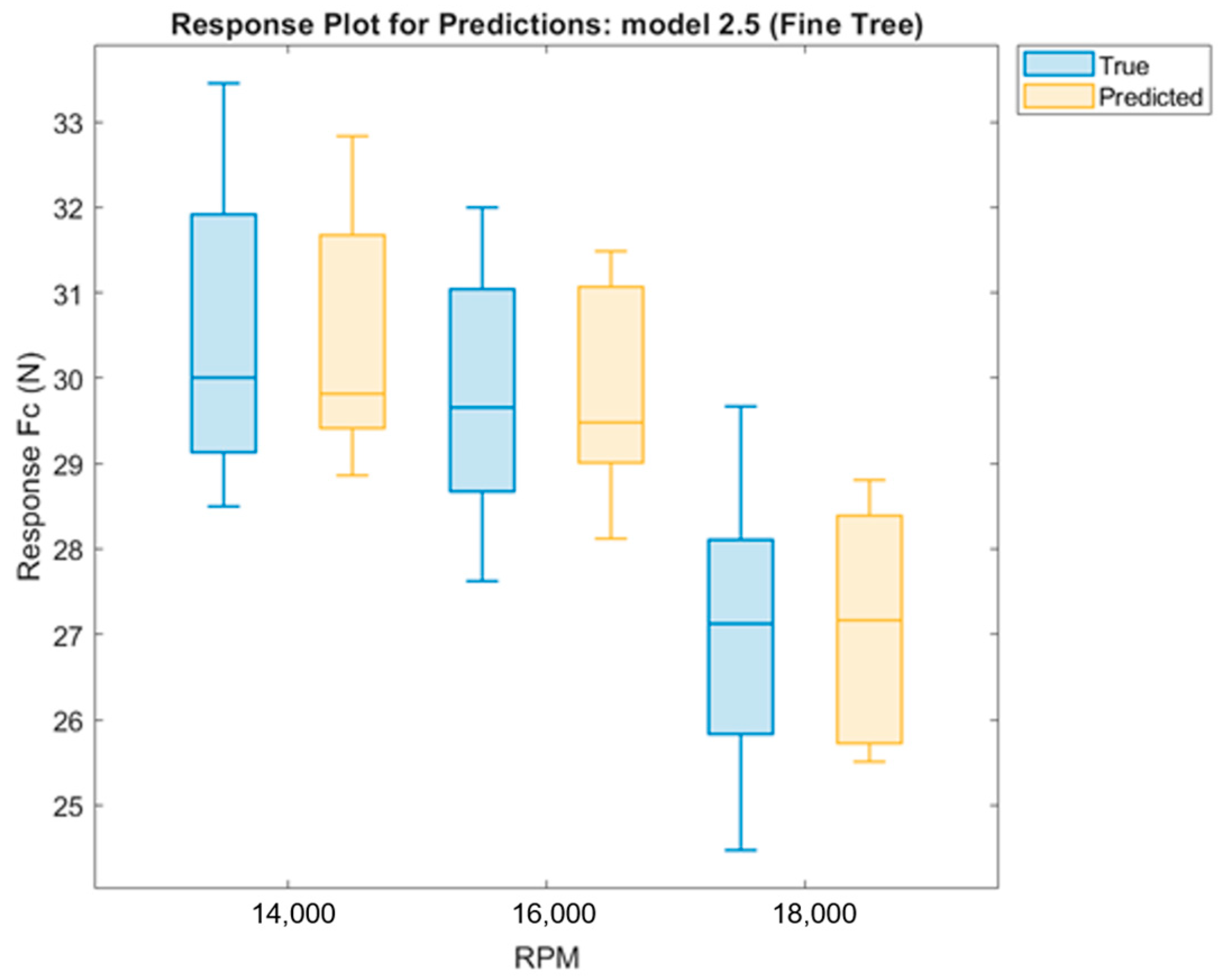
Figure 13, Figure 14 and Figure 15 show the comparison between measured and predicted values for individual predictors in box graph format. From a first look at the figures, the learned model predicts a value that is within the values of experimental measurements. The blue circle in the Figure 13 is extreme value. There is a slight shift that may be a consequence of the amount of training data. By further expanding and learning, the model can decrease in inaccuracy. It should be emphasized that not all predictors and their change appeared to be statistically significant during ANOVA analysis.

3.3. Comparison of Residual Values for Validated and Tested Data

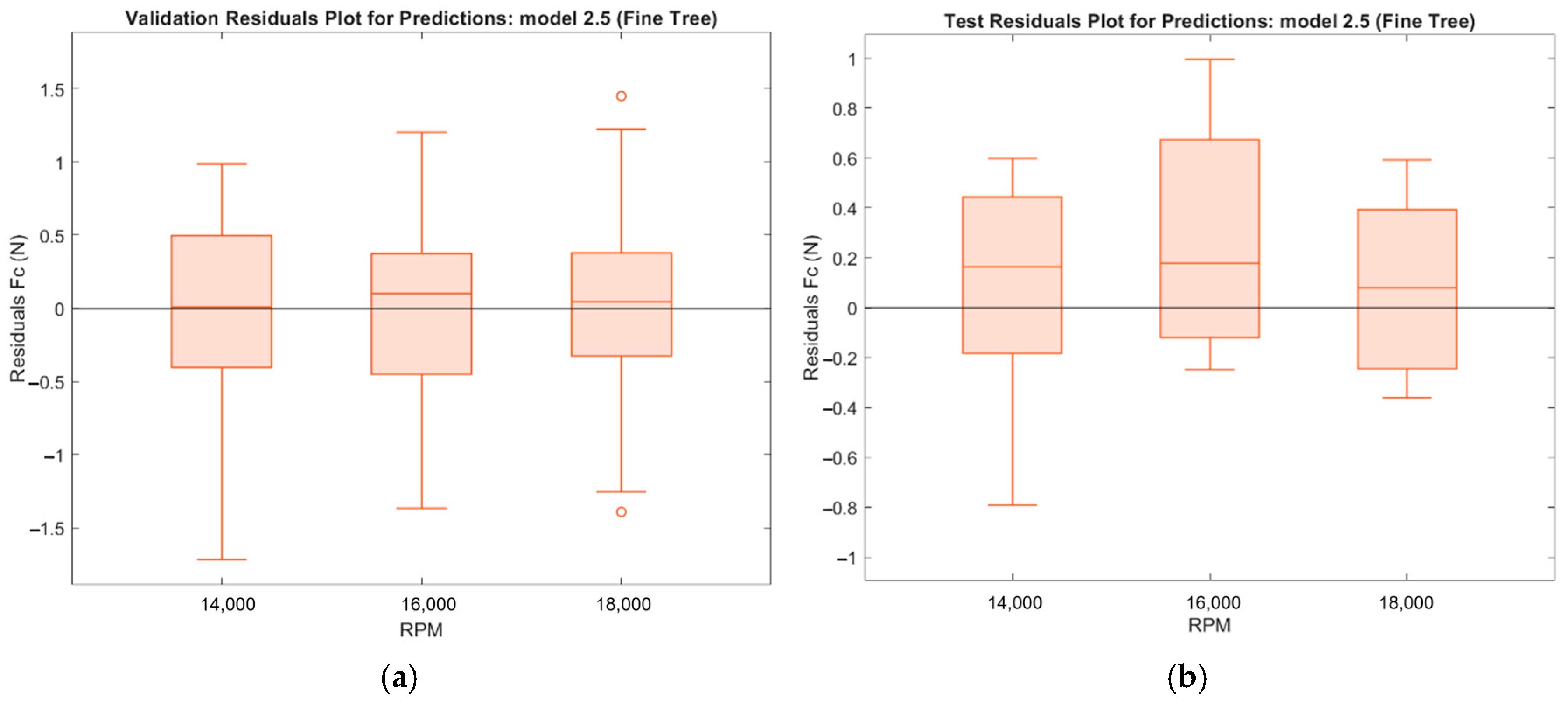
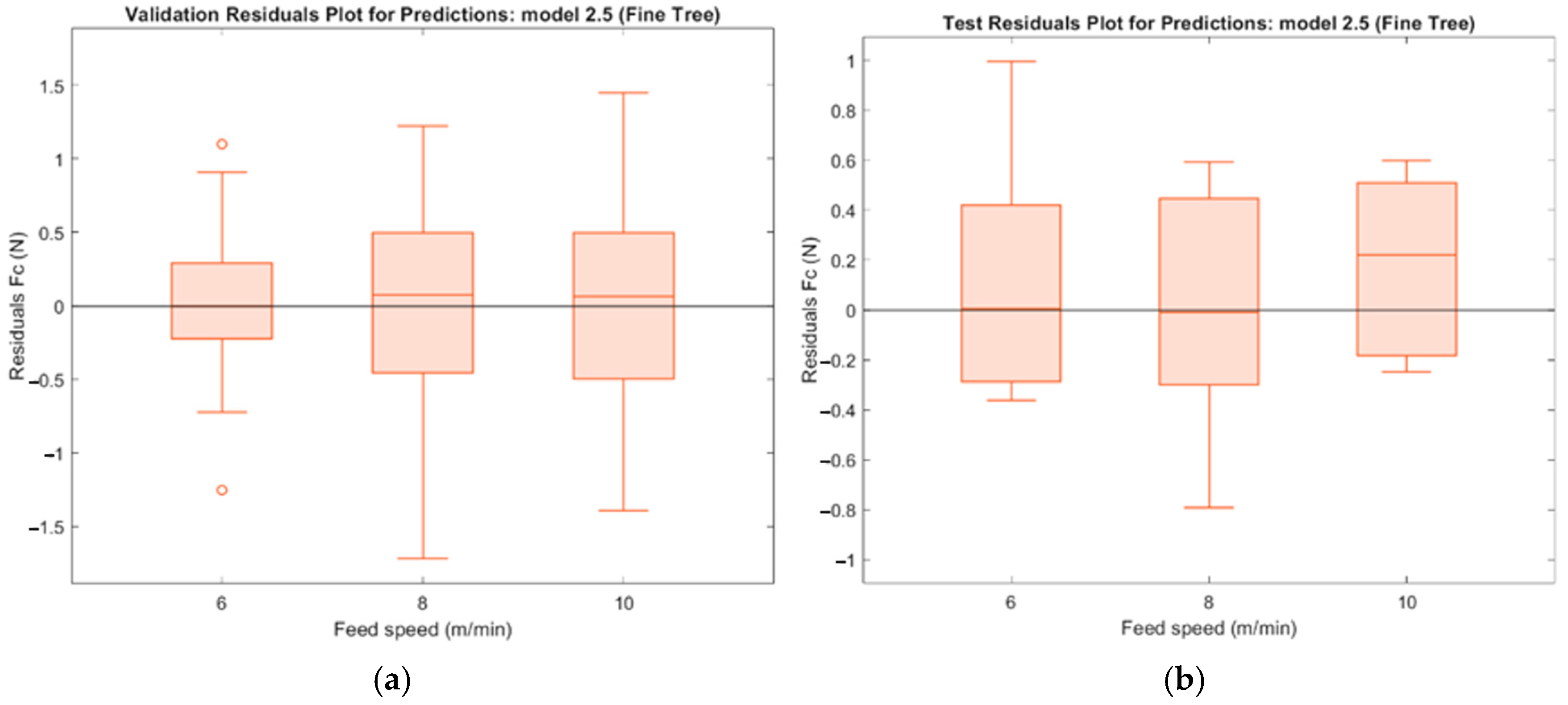
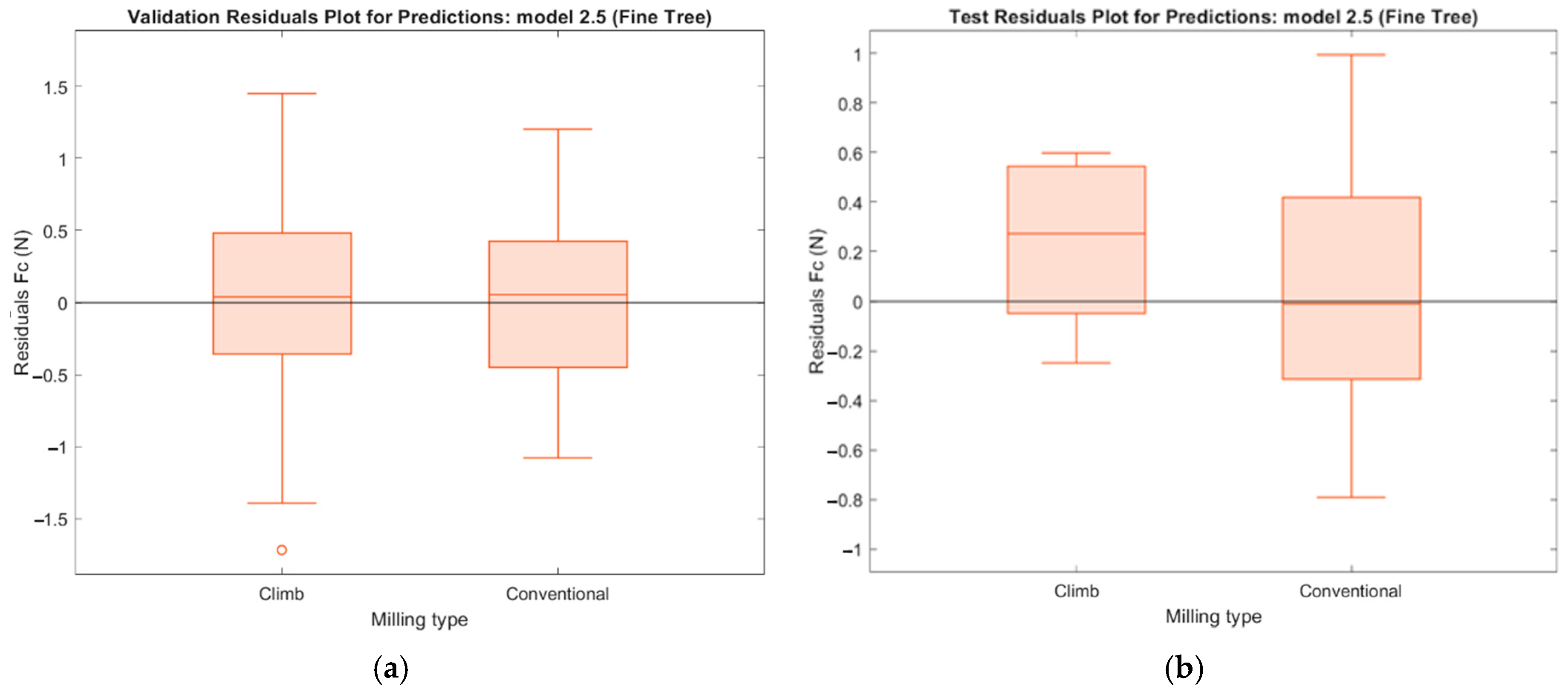
The residuals values should be randomly distributed around zero, without any visible pattern (such as a linear trend). If a pattern appears, it may indicate that the model has memorized the training data rather than learning general relationships, which limits its ability to perform well on new unseen data. The residual comparisons for the Fine Tree model (Model No. 2.5), analysed by individual predictors for the validated and tested values, are presented in Figures. It can be said that model validation was performed by comparing errors (residuals) for training and testing data. Red circles represent extreme values.

Figure 16 shows a comparison of validation residuals (a) and test residuals (b) for the RPM predictor. The distribution for validation residuals is around the zero value in the interval ±0.5 N; some extreme values are +1 and −1.5 N, respectively. The distribution for test residuals has more positive values, but also lies around a value of 0.5, i.e., corresponds to the validated residuals. This means that the model can be considered as suitably trained.

Figure 17 shows a comparison of validation residuals (a) and test residuals (b) for the feed speed predictor. The distribution for validation residuals is around the zero value in the interval ±0.5 N; some extreme values are +1.5 and −1.5 N, respectively. The test residuals are slightly shifted toward positive values; however, most of them also fall within ±0.5 N. Overall, the distribution of test residuals corresponds well to that of the validation residuals. This means that the model can be considered as suitably trained.

Figure 18 shows a comparison of validation residuals (a) and test residuals (b) for the direction of milling predictor. The distribution for validation residuals is around the zero value in the interval ±0.5 N; some extreme values are +1.5 and −1.5 N, respectively. The distribution for test residuals has more positive values, especially for climb milling. Nevertheless, most values remain within ±0.5 N, indicating that the distribution of test residuals is similar to that of the validation residuals. This means that the model can be considered as suitably trained.

4. Discussion

The presented research investigated the influences of technical and technological parameters (rotation speed of tool, feed speed of tool and type of milling) on generated forces and energetical consumption during the milling process of board materials of MDF samples. The next objective of the research was accessing the possibility of using calculated total force F_c for the purpose of developing prediction models and evaluation of their accuracy. From the point of view of evaluating the consumption of electrical energy, this does not seem to be entirely suitable for prediction models. First, the influence of technological variables on it is statistically the least pronounced. Furthermore, the consumed electrical energy and its measurement is an integral function of electrical currents and voltages, which affects its evaluation in real time.

From the perspective of force effects, individual orthogonal force components and cutting total power were evaluated. Force components were oriented according to configuration specified by the sensor manufacturer and were calculated as the absolute difference between the values measured during milling process and during idling of machine. Conventional milling exhibited lower values of the F_x component (average conventional: 15.25 N; climb: 24.79 N) and higher values of the F_y component (average conventional: 24.04 N; climb: 14.73 N). The F_z force component showed similar values regardless of the milling type (average 4.8 and 5.0 N). At the same time, the total cutting force F_c was slightly higher during climb milling (average conventional: 28.93; climb: 29.27 N), whereby similar findings have been reported by Hanincová et al. [30]. Kopecký et al. [31] also noted that climb milling demands significantly more cutting power compared to conventional milling. If the force components F_x and F_y were assessed, the type of milling has the greatest influence on their change based on the F-test (F value over 20,000). However for the calculated total cutting force, spindle speed was the most influential factor (F value 615). For power consumption, the most influential factor was also spindle speed (F value 210). It was also confirmed that power consumption increases with higher spindle speed.

All presented dependencies are related to the theory of wood composites milling, while current practical experimental knowledge is sometimes contradictory, mainly because wood and wood-based materials are heterogeneous materials. The increase in electrical power consumption is apparently due to the faster spindle rotation. The difference in total force for different types of milling is due to a different distribution of cutting forces and also a change in the cross-section of the removed layer. The change in total force when changing the spindle and feed speed is related to the fact that at higher speeds the material is cut off faster. This changes the chip thickness, and increasing the speed reduces the force required to cut it. A similar connection is found with feed rate, where increasing it increases the thickness of the cut layer per unit of time and thus the force required to remove it. Also, Moradpour et al. [32] noted significant increases in cutting forces and cutting power with higher feed speeds during composite material milling.

Model Comparison

From the point of view of assessing the suitability for the obtained data for the creation of predictive models, linear regression was chosen. This is more suitable than classic multi-layer neural networks for this type of obtained data due to their small number and individual dependencies. The models examined more closely had very similar compared features. By comparing individual models with respect to the correlation coefficient, mean square error, and training time, the most suitable type of model is Fine Tree. Similar parameters for comparing the suitability of multiple linear regression models were used in a study by Shen et al. [33] dealing with the influence of pine wood milling parameters on force effects and their prediction. Rodríguez et al. [34], Przybyś-Małaczek et al. [35], and Viswanathan et al. [36] analysed decision tree models as suitable for predicting the quality of the created surface. At the same time, Aggrogeri et al. [37] verified and tested other applications of machine learning to prevent undesirable phenomena occurring during machining, which are often modified for specific applications.

5. Conclusions

The aim of this study was to evaluate the suitability of data on cutting forces and electrical energy consumption generated during the milling of MDF boards for the development of predictive models. Although MDF boards represent a relatively homogeneous material, this characteristic did not present a limitation, particularly in the interpretation of the developed and tested model for the total cutting force F_c. In addition, the statistical significance of technological parameters with respect to the measured variables was assessed. Duncan’s post hoc test confirmed significant effects, especially for the total cutting force, across all independent variables.

The models created and tested in this study will be further developed for other forms of machining and other wood-based materials. Their practical implementation could evaluate the durability of cutting tools. At the same time, their real-time updating or the development of a modified empirical model suitable for specific conditions make predictive maintenance possible, or rather, indicate tool wear. These possibilities will be an area of further research. The main findings can be summarized as follows:

• A statistically significant effect on the measured variables was observed primarily in the force-related responses, particularly in the calculated total cutting force Fc. In contrast, for electrical energy consumption, statistically similar datasets were identified when changing spindle speed from 14,000 to 16,000 rpm and when altering the milling type (climb vs. conventional milling).
• Based on the F-test results, spindle speed exerted the greatest influence on both the total cutting force Fc and electrical energy consumption, while milling type had the smallest overall effect. For the force components in the x and y directions, the direction of milling had the most pronounced influence, which is consistent with the theoretical principles of cutting mechanics and force decomposition in an orthogonal coordinate system.
• Force effects in the z-axis direction were negligible compared to the force components in the x and y directions.
• The development of predictive models appears to be an effective approach for estimating force effects based on input technical and technological parameters. Predictive models in the form of decision trees proved to be easily interpretable and exhibited low prediction error, without indications of overfitting or underfitting.
• The developed model is straightforward to interpret and can be further extended by incorporating additional input variables.