Extended Kalman Filter-Enhanced LQR for Balance Control of Wheeled Bipedal Robots

Abstract

With the rapid development of mobile robotics, wheeled bipedal robots, which combine the terrain adaptability of legged robots with the high mobility of wheeled systems, have attracted increasing research attention. To address the balance control problem during both standing and locomotion while reducing the influence of noise on control performance, this paper proposes a balance control framework based on a Linear Quadratic Regulator integrated with an Extended Kalman Filter (KLQR). Specifically, a baseline LQR controller is designed using the robot’s dynamic model, where the control input is generated in the form of wheel-hub motor torques. To mitigate measurement noise and suppress oscillatory behavior, an Extended Kalman Filter is applied to smooth the LQR torque output, which is then used as the final control command. Filtering experiments demonstrate that, compared with median filtering and other baseline methods, the proposed EKF-based approach significantly reduces high-frequency torque fluctuations. In particular, the peak-to-peak torque variation is reduced by more than 60%, and large-amplitude torque spikes observed in the baseline LQR controller are effectively eliminated, resulting in continuous and smooth torque output. Static balance experiments show that the proposed KLQR algorithm reduces the pitch-angle oscillation amplitude from approximately ±0.03 rad to ±0.01 rad, corresponding to an oscillation reduction of about threefold. The estimated RMS value of the pitch angle is reduced from approximately 0.010 rad to 0.003 rad, indicating improved convergence and steady-state stability. Furthermore, experiments involving constant-speed straight-line locomotion and turning indicate that the KLQR algorithm maintains stable motion with velocity fluctuations limited to within ±0.05 m/s. The lateral displacement deviation during locomotion remains below 0.02 m, and no abrupt acceleration or deceleration is observed throughout the experiments. Overall, the results demonstrate that applying Extended Kalman filtering to smooth the control torque effectively improves the smoothness and stability of LQR-based balance control for wheeled bipedal robots.

1. Introduction

With the continuous advancement of mobile robotics, various novel mobile platforms such as hexapod robots [1], quadruped robots [2,3], and bipedal robots [4,5,6,7] have been developed. Owing to their superior adaptability and flexibility in unstructured environments, legged robots have gradually replaced traditional wheeled or fixed-base robots and are now widely applied in warehouse logistics, environmental monitoring, household services, and other fields [8]. However, legged robots typically feature complex control systems and exhibit limited mobility on flat terrain compared with wheeled robots, making them less efficient for smooth-surface locomotion [9]. To combine the terrain adaptability of legged mechanisms with the high mobility of wheeled platforms, hybrid wheeled–legged robots have become a major development trend, among which wheeled bipedal robots have attracted particular attention. As a typical underactuated system, the balance control of a wheeled bipedal robot forms the foundation for achieving any complex locomotion tasks [10]. Moreover, to ensure the robustness of the balance controller under various noise conditions and to mitigate oscillatory behaviors, it is essential to design a control strategy that maintains stability during both standing and walking while suppressing noise-induced fluctuations. Therefore, this study focuses on developing a balance control algorithm for wheeled bipedal robots that is applicable to both stationary and locomotion scenarios, effectively reducing noise interference and minimizing oscillations to enhance overall stability.

For the balance control of wheeled bipedal robots, existing approaches mainly include state feedback control, optimal control, nonlinear control, and adaptive control [11]. Due to its simplicity and effectiveness around equilibrium configurations, LQR has been widely applied to balance and whole-body control of wheeled bipedal robots [12]. For example, Raza et al. [13] analyzed the motion stability of wheeled-legged robots and applied an LQR controller to regulate balance, verifying through simulations the effectiveness of the LQR method for balancing wheeled-legged systems. Wang et al. [14] proposed a stationary balance controller based on a linear state feedback regulator and further introduced a nonlinear controller based on interconnection and damping assignment to enhance the disturbance rejection capability in standing balance. To address the degradation of controller performance caused by internal and external uncertainties in the dynamic model, Zhang et al. [15] developed an adaptive optimal output controller that handles model uncertainties and disturbances using a data-driven approach. Experimental results demonstrated the strong robustness of the proposed method. Cao et al. [16] linearized and discretized the dynamic model of a wheeled-legged robot around the equilibrium point, and designed a model predictive controller with input constraints to achieve balance control. An extended state observer was also introduced to enhance robustness, and results confirmed good balancing performance. Kim et al. [17] proposed an observer-based proportional controller to handle nonlinearities, parameter variations, and load uncertainties. By treating load variations and modeling errors as a lumped disturbance, the disturbance observer significantly improved the robustness of the wheeled robot controller. Qian et al. [18] proposed an adaptive machine-learning-based dynamic balance control method. Simulation results showed that without adaptive learning, the robot easily lost balance or tipped over, while the proposed approach effectively maintained the dynamic balance of a two-wheeled self-balancing robot. Xin et al. [19] developed a whole-body dynamic model by integrating torso dynamics, wheel–leg dynamics, and wheel–ground contact constraints, and proposed a whole-body control framework that successfully achieved balance control for wheeled-legged robots.

Although the aforementioned balance control methods have demonstrated satisfactory performance in point stabilization of wheeled bipedal robots, most of them have not sufficiently considered complex operating conditions such as walking and turning. Under such scenarios, external disturbances acting on the robot become more intricate, imposing stricter requirements on the robustness and stability of the controller. To address these challenges, researchers have conducted extensive studies to enhance controller robustness under complex locomotion conditions. For instance, Zhao et al. [20] proposed a compliant balance controller by integrating model predictive control with a whole-body dynamic compensator to achieve stable control during locomotion. Experimental results showed that the robot was able to withstand continuous unexpected disturbances and traverse uneven terrains such as grass and stairs smoothly. To improve the walking stability of wheeled bipedal robots, Feng et al. [21] developed a whole-body controller that combines LQR with active disturbance rejection control, and experiments demonstrated improved smoothness in locomotion. Xu et al. [22] proposed a hybrid control framework combining a Linear Quadratic Regulator and Proportional–Derivative control for wheeled bipedal robots, and experimental results demonstrated its effectiveness in achieving stable balance and locomotion. Klemm et al. [10] proposed a hierarchical whole-body controller based on full rigid-body dynamics for the Ascento robot and derived a closed-form expression of its locomotion loop dynamics. Experimental validation confirmed that the controller significantly enhanced terrain adaptability and robustness during locomotion. Wang et al. [23] presented a whole-body motion planning method capable of simultaneously regulating torso posture and maintaining full-body dynamic balance. The proposed approach was validated in a virtual environment, achieving accurate velocity and yaw-rate tracking during turning maneuvers of a wheeled bipedal robot. Li et al. [24] developed a novel hydraulic wheeled-legged robot and experimentally demonstrated its high mobility, adaptability, and robustness during flat-terrain locomotion. Cui et al. [25] investigated adaptive optimal control of wheeled-legged robots via reinforcement learning without relying on an accurate dynamic model. The controller learned from state inputs collected along robot trajectories and was verified to be effective in balancing, walking, and turning tasks. Xin et al. [26] designed a force controller based on uncertainty and disturbance estimation to precisely regulate the posture, balance, and motion of wheeled-legged robots. The controller accurately estimated and compensated for lumped uncertainties without requiring any prior information, thereby achieving effective posture control and balance stabilization.

Although the aforementioned methods improve robustness against internal and external disturbances through complex robust controllers or adaptive learning-based strategies, they considerably increase model complexity and computational cost, thereby limiting real-time applicability. In most operational scenarios of robots, noise primarily originates from onboard sensor systems and is reflected in the control inputs. Therefore, mitigating noise-induced oscillations and enhancing robustness from the perspective of control inputs offers a lower-cost and more practical solution. Among various filtering algorithms designed to suppress noise, the Extended Kalman Filter (EKF) has demonstrated superior performance compared with α–β filters [27], complementary filters [28], median filters, and moving average filters, and has thus been widely adopted in robotic control applications [29]. For instance, Sun et al. [30] combined Kalman filtering with an LQR controller for a two-wheeled self-balancing robot, where the Kalman filter effectively reduced sensor measurement noise and computational burden; experimental results demonstrated strong disturbance rejection and balance stability. Laddach et al. [31] achieved stable control of a two-wheeled balancing robot using measurement filtering, fusing data from a gyroscope, accelerometer, and encoder, and applying a Kalman filter to obtain stable performance. Srichandan et al. [32] employed an Extended Kalman Filter to process sensor data, feeding the filtered output into a reinforcement learning framework to construct a stabilization controller for a two-wheeled self-balancing robot; experiments confirmed that the EKF-based controller achieved superior robustness. Choudhry et al. [33] developed a controller integrating an Extended Kalman Filter with a sliding mode control strategy, and experiments showed that the EKF-enhanced controller achieved zero steady-state error without overshoot, improving the performance of the sliding mode controller and addressing stability challenges. Similarly, Herrera et al. [34] used an Extended Kalman Filter to eliminate gyroscope noise and subsequently designed a fuzzy optimal controller for balance control of a two-wheeled robot, thereby improving robustness and reducing steady-state error.

Based on the above research, this paper proposes an LQR-based balance control algorithm integrated with an Extended Kalman Filter (EKF) for a wheeled bipedal robot. The proposed method aims to address the degradation of stability and robustness in standing and walking balance control caused by noise interference, while improving controller performance and reducing overall complexity.

The main contributions of this paper are summarized as follows:

• To address the limitation that conventional wheeled and legged robots cannot simultaneously achieve terrain adaptability and high mobility, a wheeled bipedal robot is designed by integrating the advantages of both locomotion modes. For the standing and walking balance control problem, an LQR-based balance control algorithm is developed based on the robot’s dynamic model. Considering the presence of various noise sources during motion and aiming to reduce controller complexity, the EKF is incorporated to smooth the LQR control torque. Accordingly, a KLQR balance control algorithm combining EKF and LQR is proposed, where the EKF is applied to the LQR-generated control torque rather than to the system state, in order to enhances the smoothness and robustness of the robot’s motion.
• An experimental platform is established, consisting of the wheeled bipedal robot, an IMU sensing system, and an industrial PC with a real-time operating system. Comparative experiments with different filtering algorithms demonstrate that the integrated the EKF effectively suppresses spikes in the control torque. Furthermore, experimental results verify that the proposed KLQR balance control algorithm mitigates steady-state oscillations, improves robustness, and maintains excellent performance during walking and turning maneuvers at various speeds.

It should be noted that the contribution of this work is not to introduce a new control or filtering algorithm, but to systematically investigate the practical effectiveness of EKF-based control torque smoothing within an LQR balance control framework for wheeled bipedal robots, with a focus on real-time implementation and experimental validation.

The overall structure of this paper is organized as follows. In Section 2, the dynamic model of the robot is established based on Newtonian mechanics, and an LQR balance controller is designed by formulating the corresponding state-space representation. In Section 3, to suppress control torque spikes and alleviate robot oscillations, thereby improving stability and robustness, an Extended Kalman Filter is integrated with the LQR controller to develop a robust KLQR control strategy, and the effectiveness of the filtering method is validated through performance evaluations. In Section 4, an experimental platform for in-place balancing as well as walking and turning control of the wheeled bipedal robot is constructed, and the performance of the proposed algorithm in real-world balance control is analyzed. Finally, Section 5 presents the conclusions of this paper. The overall framework of the paper is illustrated in Figure 1.

2. LQR Balance Control Algorithm for Wheeled Bipedal Robots Based on the Dynamic Model

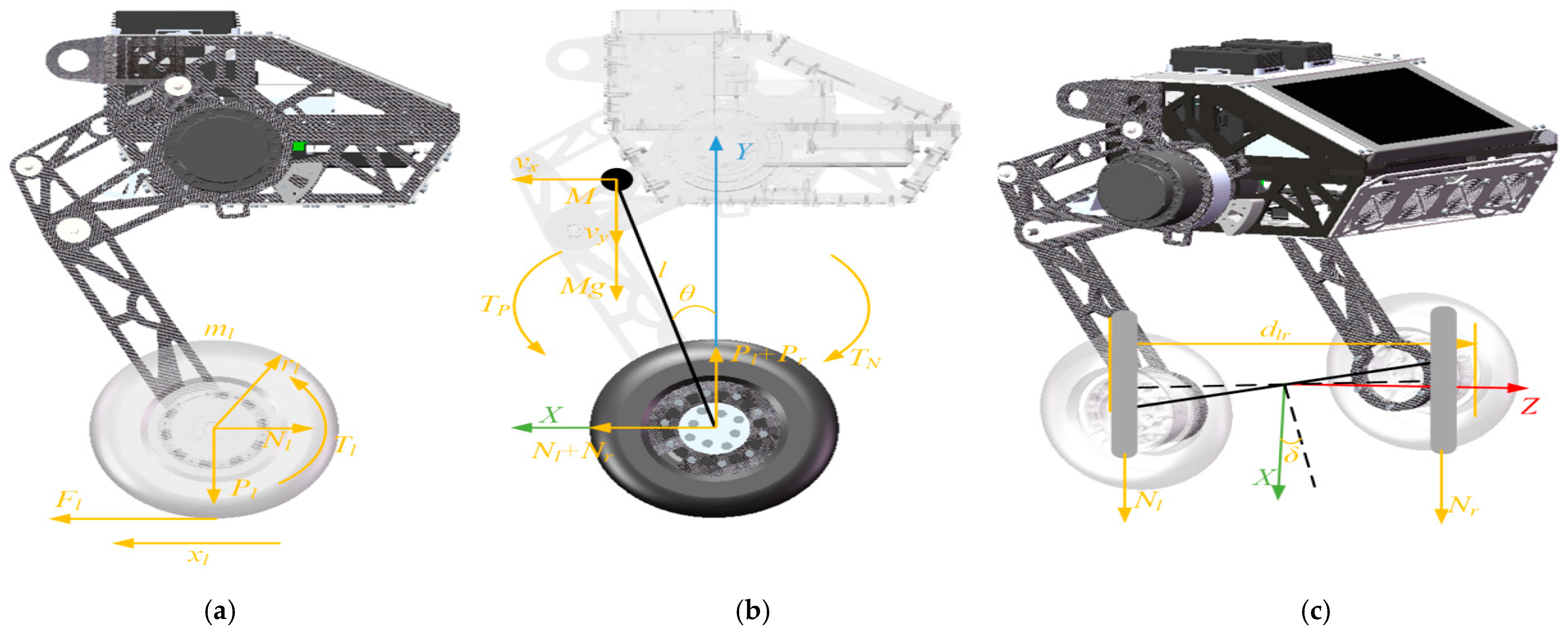
2.1. Dynamic Model Based on Newtonian Mechanics

As shown in Figure 1, to design a balance controller based on the robot’s dynamic model, it is first necessary to establish the dynamic model of the wheeled bipedal robot. For the balance control problem considered in this study, the following idealized assumptions are made: (1) the chassis mass is concentrated at the center of mass; (2) the influence of leg motion is neglected; and (3) the driving wheels roll on the ground without slipping. Based on these assumptions, the balance control model of the wheeled bipedal robot can be equivalently represented as a two-wheeled inverted pendulum with a variable pendulum length. The entire system can be divided into three components—the left driving wheel, the right driving wheel, and the chassis—and the force analysis for each component is illustrated in Figure 2.

From Figure 2, by considering the force balance along the x-direction and the torque balance about the wheel axle, the dynamic relationship of the left driving wheel can be obtained as:

$$T_l-\left(m_l{\ddot{x}}_l+N_l\right)r_l=I_l{\dot{\omega }}_l,$$

(1)

where $F_l$ is the friction force between the left driving wheel and the ground, $N_l$ is the horizontal reaction force exerted by the chassis on the left driving wheel, $m_l$ is the mass of the left driving wheel, and $x_l$ is the displacement of the left driving wheel along the x-direction. $T_l$ is the driving torque applied to the left driving wheel, $r_l$ is its radius, $I_l$ is the moment of inertia of the left driving wheel about its axle, and ${\omega }_l$ is the angular velocity of the wheel.

Furthermore, since the driving wheels undergo rolling without slipping relative to the ground, the angular acceleration can be expressed in terms of the linear acceleration and the wheel radius, yielding the dynamic equations of the left driving wheels:

$${\ddot{x}}_l={\displaystyle \frac{T_l{r}_l - N_l{r_l}^2}{I_l + m_l{r_l}^2}},$$

(2)

The dynamic equation of the right driving wheel can be obtained similarly as:

$${\ddot{x}}_r={\displaystyle \frac{T_r{r}_r - N_r{r_r}^2}{I_r + m_r{r_r}^2}},$$

(3)

where $x_r$ is the displacement of the right driving wheel along the x-direction, $T_r$ is the driving torque applied to the right wheel, $r_r$ is the wheel radius, $N_r$ is the horizontal reaction force exerted by the chassis, $I_r$ is the wheel’s moment of inertia about its axle, and $m_r$ is the wheel mass.

The acceleration of the chassis, ${\ddot{x}}_b$, is the average of the left and right driving wheel axle accelerations, i.e.,

$${\ddot{x}}_b={\displaystyle \frac{{\ddot{x}}_l+{\ddot{x}}_r}{2}},$$

(4)

Considering the chassis center of mass as the reference for force analysis, the horizontal forces $N_l$, $N_l$ and vertical forces $P_l$, $P_r$ applied at the wheels can be transferred to the center of mass, generating additional torques $T_N$ and $T_P$ as:

$$T_N=\left(N_l+N_r\right)lcos\theta ,$$

(5)

$$T_P=\left(P_l+P_r\right)lsin\theta ,$$

(6)

where $l$ is the distance from the center of mass to the center of the driving wheels, and $\theta$ is the angle between the vertical direction and the line connecting the center of mass to the wheel centers.

Decomposing the absolute velocity at the center of mass into x and y components gives.

$$v_x={\dot{x}}_b+{\displaystyle \frac{d\left(lsin\theta \right)}{dt}}={\dot{x}}_b+l\dot{\theta }cos\theta ,$$

(7)

$$v_y={\displaystyle \frac{d\left(l-lcos\theta \right)}{dt}}=l\dot{\theta }sin\theta ,$$

(8)

Based on the velocity expressions of the chassis center of mass given in Equations (7) and (8), the resultant forces acting on the chassis can be expressed directly in terms of the translational and rotational accelerations.

Specifically, the force balance along the x-direction yields:

$$N_l+N_r=M({\ddot{x}}_b+l\ddot{\theta }cos\theta -l{\dot{\theta }}^{2}sin\theta ),$$

(9)

Similarly, the force balance along the y-direction of the chassis center of mass is given by:

$$Mg-P_l-P_r=M(l\ddot{\theta }sin\theta +l{\dot{\theta }}^{2}cos\theta ),$$

(10)

Analyzing the torque of the chassis about the z-axis yields the moment balance equation:

$$J_z\ddot{\theta }=T_P-T_N-T_l-T_r,$$

(11)

where $J_z$ is the moment of inertia of the chassis about the z-axis.

Substituting Equations (5) and (6), Equations (9) and (10) into Equation (11) and simplifying results in the dynamic equation of the chassis:

$$\left(J_z+M{l}^2\right)\ddot{\theta }=Mglsin\theta -Ml{\ddot{x}}_{b}cos\theta -T_l-T_r,$$

(12)

Substituting Equation (9) into Equation (4) gives the complete dynamic equation of the driving wheels:

$$\left(2I_l+2m{r_l}^2+M{r_l}^2\right){\ddot{x}}_b=T_l{r}_l+T_r{r}_l+M{r_l}^{2}l{\dot{\theta }}^{2}sin\theta -M{r_l}^{2}l\ddot{\theta }cos\theta ,$$

(13)

When the chassis tilt angle is small, i.e., the robot maintains balance near the equilibrium position within a small angular range, the following linearization can be applied: $cos\theta =1$, $sin\theta =\theta$, ${\dot{\theta }}^2=0$. Therefore, linearizing Equations (12) and (13) yields the dynamic equations of the Wheeled bipedal robot for balance control:

$$\{\begin{array}{l}\left(J_z+M{l}^2\right)\ddot{\theta }=Mgl\theta -Ml{\ddot{x}}_b-T_l-T_r\\ \left(2I_l+2m{r_l}^2+M{r_l}^2\right){\ddot{x}}_b=T_l{r}_l+T_r{r}_l-M{r_l}^{2}l\ddot{\theta }\end{array},$$

(14)

After establishing the dynamics of straight-line motion, the turning dynamics of the robot are considered. The robot achieves turning through the differential motion of the left and right driving wheels, which generates a yaw moment acting on the chassis. By relating the differential wheel accelerations to the yaw angular acceleration and combining the wheel dynamics, the turning dynamics of the robot can be expressed as:

$$\ddot{\delta }={\displaystyle \frac{\ddot{x_l }-\ddot{ x_r}}{d_{lr}}}={\displaystyle \frac{d_{lr}{r}_l{T}_l - d_{lr}{r}_l{T}_r}{m_r{d_{lr}}^2{r_l}^2 + I_l{d_{lr}}^2 + 2J_y{r_l}^2}},$$

(15)

where $J_y$ is the moment of inertia of the chassis about the y-axis, $\delta$ is the yaw angle.

Based on the established dynamic models of straight-line and turning motion, the robot’s state-space representation can be derived. By combining Equations (14) and (15) and grouping similar terms, we obtain an intermediate set of dynamic relations, which forms part of the state-space representation of the robot.

$$\{\begin{array}{l}{\ddot{x}}_b=\left(T_l+T_r-c_2\ddot{\theta }\right)/c_1\\ \ddot{\theta }={(c}_4\theta -c_5\ddot{x_b}-T_l-T_r)/c_3\\ \ddot{\delta }=c_6{T}_l-c_6{T}_r\end{array}$$

(16)

The coefficients in Equation (16) satisfy the following relationships:

$$\{\begin{array}{l}{c}_1=\left(2I_l+2m{r_l}^2+M{r_l}^2\right)/r_l\\ c_2=M{r}_{l}l\\ c_3=J_z+M{l}^2\\ c_4=Mgl\\ c_5=Ml\\ c_6=d_{lr}{r}_l/\left(m_r{d_{lr}}^2{r_l}^2+I_l{d_{lr}}^2+2J_y{r_l}^2\right)\end{array},$$

(17)

The physical parameters of the wheeled bipedal robot are listed in

Table 1. The physical parameters of the wheeled bipedal robot.

Physical Parameters	Value
m	0.895 kg
M	10.914 kg
$I_l$	257.18 mm
$r_l$	102.5 mm
$l$	0.0031 kg × ${\mathrm{m}}^2$
$J_y$	0.3998 kg × ${\mathrm{m}}^2$
$J_z$	0.5277 kg × ${\mathrm{m}}^2$

, and the meanings of the corresponding symbols have been discussed above.

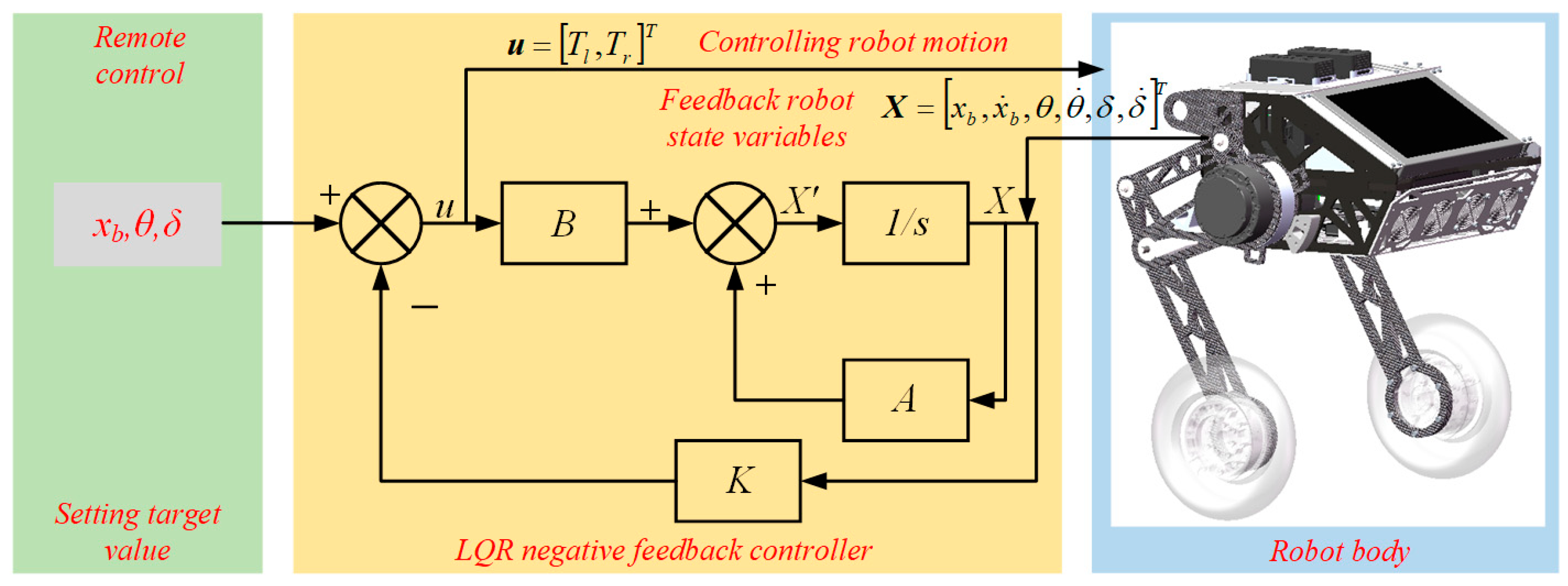
2.2. LQR Balance Control Algorithm Based on the Dynamic Model

Based on Figure 1, a balance motion controller can be constructed from the established dynamic model. To achieve effective motion control, appropriate state variables and control variables must be selected. According to the robot motion control requirements in this study, the robot primarily involves three states: forward/backward motion, turning, and standing balance. To obtain good control performance, six variables are selected as the state variables, including the robot’s position, pitch angle, yaw angle, and their corresponding velocity components. Therefore, the state vector X can be expressed as:

$$\mathit{X}={\left[x_b,{\dot{x}}_b,\theta ,\dot{\theta },\delta ,\dot{\delta }\right]}^T,$$

(18)

The control is implemented by regulating the torque applied to the two driving wheels; thus, the control vector u can be expressed as:

$$\mathit{u}={\left[T_l,T_r\right]}^T,$$

(19)

Combining Equations (18) and (19), the state-space representation is:

$$\{\begin{array}{c}\dot{\mathit{X}}=\mathit{A}\mathit{X}+\mathit{B}\mathit{u},\\ Y= \mathit{u}\end{array}$$

(20)

where A is a 6 × 6 coefficient matrix representing the relationships among the system’s internal state variables, and B is a 6 × 2 control matrix representing the effect of the inputs on each state variable.

Based on the state-space formulation in Equation (20), Equation (16) can be rearranged into the following set of second-order dynamic relations, which forms part of the state-space model construction:

$$\{\begin{array}{l}{\ddot{x}}_b={\displaystyle \frac{-c_2{c}_4}{c_1{c}_3-c_2{c}_5}}\theta +{\displaystyle \frac{c_2+c_3}{c_1{c}_3-c_2{c}_5}}\left(T_l+T_r\right)\\ \ddot{\theta }={\displaystyle \frac{c_1{c}_4}{c_1{c}_3-c_2{c}_5}}\theta -{\displaystyle \frac{c_1+c_5}{c_1{c}_3-{\mathrm{c}}_2{c}_5}}\left(T_l+T_r\right)\\ \ddot{\delta }=c_6\left(T_l-T_r\right)\end{array},$$

(21)

From Equations (20) and (21), the state-space matrix form can be expressed as:

$$\{\begin{array}{c}\left[\begin{array}{c}{\dot{x}}_b\\ {\ddot{x}}_b\\ \dot{\theta }\\ \ddot{\theta }\\ \dot{\delta }\\ \ddot{\delta }\end{array}\right]=\left[\begin{array}{cccccc}0& 1& 0& 0& 0& 0\\ 0& 0& A_{23}& 0& 0& 0\\ 0& 0& 0& 1& 0& 0\\ 0& 0& A_{43}& 0& 0& 0\\ 0& 0& 0& 0& 0& 1\\ 0& 0& 0& 0& 0& 0\end{array}\right]\left[\begin{array}{c}{x}_b\\ {\dot{x}}_b\\ \theta \\ \dot{\theta }\\ \delta \\ \dot{\delta }\end{array}\right]+\left[\begin{array}{cc}0& 0\\ B_{21}& B_{22}\\ 0& 0\\ B_{41}& B_{42}\\ 0& 0\\ B_{61}& B_{62}\end{array}\right]\left[\begin{array}{c}{T}_l\\ T_r\end{array}\right]\\ \left[\begin{array}{c}{y}_l\\ y_r\end{array}\right]=\left[\begin{array}{cc}1& 0\\ 0& 1\end{array}\right]\left[\begin{array}{c}{T}_l\\ T_r\end{array}\right]\end{array},$$

(22)

The state vector X is obtained from robot sensor measurements, while matrices A and B are fully determined by the robot’s mass properties. The parameters satisfy the following relations:

$$\{\begin{array}{c}{A}_{23}={\displaystyle \frac{-c_2{c}_4}{c_1{c}_3-c_2{c}_5}}\\ A_{43}={\displaystyle \frac{c_1{c}_4}{c_1{c}_3-c_2{c}_5}}\\ B_{21}=B_{22}={\displaystyle \frac{c_2+c_3}{c_1{c}_3-c_2{c}_5}}\\ B_{41}=B_{42}=-{\displaystyle \frac{c_1+c_5}{c_1{c}_3-c_2{c}_5}}\\ B_{61}=c_6\\ B_{62}=-c_6\end{array},$$

(23)

To achieve balance control of this inherently unstable system, a state-feedback controller is designed based on the state-space representation to ensure closed-loop stability. The Linear Quadratic Regulator (LQR), as a full-state feedback controller, is widely employed in state-space-based control applications [35]. LQR computes an optimal feedback gain matrix to derive the linear optimal control law. Based on the full-state feedback property of LQR and Equation (20), the resulting control architecture is illustrated in Figure 3.

According to Figure 3, to achieve the desired stability performance, the state-feedback controller is designed as:

$$\mathit{u}=-\mathit{K}\mathit{X},$$

(24)

Combining Equations (20) and (24) gives:

$$\dot{\mathit{X}}=\left(\mathit{A}-\mathit{{\rm B}}\mathit{K}\right)\mathit{X}={\mathit{A}}_{\mathit{c}}\mathit{X},$$

(25)

where K is the 2 × 6 feedback matrix.

To maintain the Wheeled bipedal robot system in a stable state, the elements of K must be adjusted such that all eigenvalues of ${\mathit{A}}_{\mathit{c}}$ are non-positive. To configure the poles for optimal control performance, an objective cost function J is introduced for the LQR balance controller:

$$J={\displaystyle \frac{1}{2}}{\int }_0^{\infty }\left({\mathit{X}}^{\mathit{T}}\mathit{Q}\mathit{X}+{\mathit{u}}^{\mathit{{\rm T}}}\mathit{R}\mathit{u}\right)dt,$$

(26)

where Q is a 6 × 6 semi-positive definite matrix representing the penalty on the state variables, and R is a 2 × 2 positive definite matrix representing the penalty on the control input u. A larger entry in matrix Q indicates that the corresponding state variable converges to zero more rapidly; similarly, each entry in matrix R corresponds to the magnitude of a particular control input. Therefore, according to Equation (26), the optimization process aims to minimize the cost function by tuning matrices Q and R. Since matrices Q and R are associated with the state variable X and control input u, respectively, the objective is to adjust the state-feedback controller in Equation (24) such that the cost function is minimized, which is manifested as finding the optimal feedback gain matrix K. By substituting Equation (24) into Equation (26), we obtain:

$$J={\displaystyle \frac{1}{2}}{\int }_0^{\infty }{\mathit{X}}^{\mathit{T}}\left(\mathit{Q}+{\mathit{K}}^{\mathit{{\rm T}}}\mathit{R}\mathit{K}\right)\mathit{X}dt,$$

(27)

Assuming the existence of a symmetric semi-positive definite constant matrix P such that:

$${\displaystyle \frac{d}{dt}}\left({\mathit{X}}^T\mathit{P}\mathit{X}\right)=-{\mathit{X}}^{\mathit{T}}\left(\mathit{Q}+{\mathit{K}}^{\mathit{{\rm T}}}\mathit{R}\mathit{K}\right)\mathit{X},$$

(28)

Differentiating the left-hand side of Equation (28) yields:

$${\dot{\mathit{X}}}^{\mathit{T}}\mathit{P}\mathit{X}+{\mathit{X}}^{\mathit{T}}\mathit{P}\dot{\mathit{X}}=-{\mathit{X}}^{\mathit{T}}\left(\mathit{Q}+{\mathit{K}}^{\mathit{{\rm T}}}\mathit{R}\mathit{K}\right)\mathit{X},$$

(29)

Substituting Equation (25) into Equation (29) and simplifying results in:

$${\mathit{A}}^{\mathit{T}}\mathit{P}+\mathit{P}\mathit{A}+\mathit{Q}-{\mathit{K}}^{\mathit{T}}{\mathit{B}}^{\mathit{T}}\mathit{P}-\mathit{P}\mathit{B}\mathit{K}+{\mathit{K}}^{\mathit{T}}\mathit{R}\mathit{K}=0,$$

(30)

In Equation (30), A, B, Q, R, and P are constant matrices, and only K is variable. Therefore, the optimization problem reduces to finding a matrix K that minimizes the cost function. By transforming the K-dependent part into a structure similar to ${\left(\mathit{M}+\mathit{N}\right)}^T\left(\mathit{M}+\mathit{N}\right)$, the cost function is minimized when M + N = 0, yielding the matrix K.

Since R is symmetric positive definite, a shift matrix can be found such that $\mathit{R}={\mathit{T}}^{\mathit{T}}\mathit{T}$ satisfies the condition, and substituting it into Equation (30) gives:

$${\mathit{A}}^{\mathit{T}}\mathit{P}+\mathit{P}\mathit{A}+\mathit{Q}-{\mathit{K}}^{\mathit{T}}{\mathit{B}}^{\mathit{T}}\mathit{P}-\mathit{P}\mathit{B}\mathit{K}+{\mathit{K}}^{\mathit{T}}{\mathit{T}}^T\mathit{T}\mathit{K}=0,$$

(31)

By applying the method of undetermined coefficients to transform the K-dependent term $-{\mathit{K}}^{\mathit{T}}{\mathit{B}}^{\mathit{T}}\mathit{P}-\mathit{P}\mathit{B}\mathit{K}+{\mathit{K}}^{\mathit{T}}{\mathit{T}}^T\mathit{T}\mathit{K}$ into the target form ${\mathit{M}}^T\mathit{M}+{\mathit{M}}^T\mathit{N}+{\mathit{N}}^T\mathit{M}+{\mathit{N}}^T\mathit{N}$, we obtain:

$$\{\begin{array}{l}\mathit{M}=-{\left({\mathit{T}}^{-1}\right)}^T{\mathit{B}}^T\mathit{P}\\ \mathit{N}=\mathit{T}\mathit{K}\end{array},$$

(32)

Thus, the K-dependent part can be expressed as:

$$-{\mathit{K}}^{\mathit{T}}{\mathit{B}}^{\mathit{T}}\mathit{P}-\mathit{P}\mathit{B}\mathit{K}+{\mathit{K}}^{\mathit{T}}{\mathit{T}}^T\mathit{T}\mathit{K}={\left(\mathit{M}+\mathit{N}\right)}^T\left(\mathit{M}+\mathit{N}\right)-\mathit{P}\mathit{B}{\mathit{R}}^{-1}{\mathit{B}}^T\mathit{P},$$

(33)

When M + N = 0, we have:

$$\mathit{T}\mathit{K}-{\left({\mathit{T}}^{-1}\right)}^T{\mathit{B}}^T\mathit{P}=0,$$

(34)

Solving Equation (34) yields:

$$\mathit{K}={\mathit{R}}^{-1}{\mathit{B}}^T\mathit{P},$$

(35)

Substituting Equation (35) into Equation (31) and simplifying gives:

$${\mathit{A}}^{\mathit{T}}\mathit{P}+\mathit{P}\mathit{A}+\mathit{Q}-\mathit{P}\mathit{B}{\mathit{R}}^{-1}{\mathit{B}}^T\mathit{P}=0,$$

(36)

By selecting appropriate matrices Q and R and substituting them into Equation (36), the matrix P can be obtained. Then, substituting P into Equation (35) yields the optimal feedback matrix K corresponding to the chosen Q and R. Combining matrix K with the current state variables of the Wheeled bipedal robot allows computation of the control vector for the next time step, achieving balance control.

The linearized model and the corresponding LQR controller are designed around the upright equilibrium configuration and are primarily valid for balance control scenarios involving small-to-moderate attitude deviations.

3. Data Smoothing Using Extended Kalman Filter

3.1. Principle of Data Smoothing with Extended Kalman Filter

In Section 2, an LQR balance control algorithm was proposed based on the dynamic model of the wheeled bipedal robot. The algorithm computes the robot’s control input by integrating real-time measurements from motor encoders and attitude sensors. However, during actual operation, these measurements inevitably contain noise, which can result in inaccurate or highly fluctuating control inputs, severely compromising the robot’s stability. Moreover, the accumulation of errors across different state variables can further amplify noise, degrading control performance. To address this issue, the EKF is incorporated into the LQR controller output to smooth the control signals and mitigate the effects of measurement noise.

It should be noted that, unlike the conventional application of the Extended Kalman Filter for system state estimation, the EKF in this work is employed to smooth the control torque generated by the LQR controller. The motivation for this design lies in the limitations of traditional low-pass filters (LPFs) when applied to balance control of wheeled bipedal robots. Specifically, LPFs rely on fixed cutoff frequencies and may introduce undesired phase delays, which can degrade control responsiveness and negatively affect balance stability.

For clarity, it is emphasized that the proposed KLQR framework differs fundamentally from the conventional Linear Quadratic Gaussian (LQG) control architecture. In LQG control, the Kalman filter is used to estimate the system states, which are subsequently fed into the LQR controller. In contrast, the EKF in this work does not participate in state estimation. Instead, it is employed as a control-output filtering mechanism, operating on the torque signal generated by the LQR controller. This design choice allows effective suppression of torque spikes and high-frequency fluctuations without altering the original LQR state-feedback structure.

In the proposed KLQR framework, the EKF leverages a model-based prediction–correction mechanism to filter the control output in the time domain. The EKF state is defined as the control torque applied to the wheel-hub motors, whose temporal evolution is described by a discrete-time system model with process noise accounting for unmodeled dynamics and external disturbances. The measurement corresponds to the raw LQR control torque, which is treated as a noisy observation due to sensor noise and numerical differentiation. By explicitly modeling the torque evolution and noise characteristics, the EKF effectively suppresses high-frequency fluctuations and eliminates abrupt torque spikes while preserving control continuity and responsiveness.

For real-time control of the wheeled bipedal robot, the LQR control input for the next time step can be either predicted from the previous state or computed directly from the current state measurements. Both approaches, however, are subject to uncertainty. The Extended Kalman Filter serves to optimally fuse these two estimates, thereby reducing system uncertainty and improving the accuracy of the control input [36].

For the implementation of the Extended Kalman Filter, the continuous-time model is discretized, yielding the discrete-time state equation with the state transition matrix ${\mathit{A}}_{\mathit{k}}$.

Considering the state obtained from the state transition equation to compute the LQR control input, the system state description can be expressed as:

$$\mathit{x}\left(\mathit{k}\right)={\mathit{A}}_{\mathit{k}}\mathit{x}\left(\mathit{k}-1\right)+\mathit{w}\left(\mathit{k}\right),$$

(37)

where $\mathit{x}\left(\mathit{k}\right)={\left[T_{lk},T_{rk}\right]}^T$ represents the system state vector at time step k, including the control torques of the left and right driving wheels; $A_k$ is a 2 × 2 state transition matrix, which in this system equals the identity matrix; $\mathit{x}\left(\mathit{k}-1\right)={\left[T_{l(k-1)},T_{r(k-1)}\right]}^T$ is the system state vector at time step k − 1; $\mathit{w}\left(\mathit{k}\right)$ is a 2 × 1 process noise vector following zero-mean Gaussian white noise, i.e., $\mathit{w}\left(\mathit{k}\right)~N\left(0,{\mathit{Q}}_{\mathit{k}}\right)$, where ${\mathit{Q}}_{\mathit{k}}$ is the covariance matrix of the process noise.

Considering the state obtained from the measurement system to compute the LQR control input, the system measurement description can be expressed as:

$$\mathit{z}\left(\mathit{k}\right)=\mathit{H}\mathit{x}\left(\mathit{k}\right)+\mathit{v}\left(\mathit{k}\right),$$

(38)

where $\mathit{z}\left(\mathit{k}\right)={\left[T_{lk},T_{rk}\right]}^T$ is the LQR control vector computed from the measured state variables at time step k; H is a 2 × 2 observation matrix, which in this system equals the identity matrix; $\mathit{v}\left(\mathit{k}\right)$ is a 2 × 1 measurement noise vector, also following zero-mean Gaussian white noise, i.e., $\mathit{v}\left(\mathit{k}\right)~N\left(0,{\mathit{R}}_{\mathit{k}}\right)$, where ${\mathit{R}}_{\mathit{k}}$ is the covariance matrix of the measurement noise.

According to Equation (37), assuming the system estimate at time k − 1 is $\widehat{x}\left(k-1|k-1\right)$, with its covariance $\widehat{P}\left(k-1|k-1\right)$, the predicted state $\widehat{x}\left(k|k-1\right)$ at time k can be obtained as:

$$\widehat{\mathit{x}}\left(\mathit{k}|\mathit{k}-1\right)={\mathit{A}}_{\mathit{k}}\widehat{\mathit{x}}\left(\mathit{k}-1|\mathit{k}-1\right),$$

(39)

The covariance of the predicted state $\mathit{P}\left(\mathit{k}|\mathit{k}-1\right)$ is given by:

$$\mathit{P}\left(\mathit{k}|\mathit{k}-1\right)={\mathit{A}}_{\mathit{k}}\mathit{P}\left(\mathit{k}-1|\mathit{k}-1\right){{\mathit{A}}_{\mathit{k}}}^T+\mathit{Q}\left(\mathit{k}\right),$$

(40)

Combining Equations (38) and (39), the measurement variance can be expressed as:

$$\mathit{y}\left(\mathit{k}\right)=\mathit{z}\left(\mathit{k}\right)-\mathit{H}\widehat{\mathit{x}}\left(\mathit{k}|\mathit{k}-1\right),$$

(41)

The covariance of the measurement residual $\mathit{S}\left(\mathit{k}\right)$ is:

$$\mathit{S}\left(\mathit{k}\right)=\mathit{H}\mathit{P}\left(\mathit{k}|\mathit{k}-1\right){\mathit{H}}^{\mathit{T}}+\mathit{R}\left(\mathit{k}\right),$$

(42)

Thus, when the gain is $\mathit{K}\left(\mathit{k}\right)$, the optimal state estimate $\widehat{\mathit{x}}\left(\mathit{k}|\mathit{k}\right)=\widehat{\mathit{x}}\left(\mathit{k}|\mathit{k}-1\right)+\mathit{K}\left(\mathit{k}\right)\mathit{y}\left(\mathit{k}\right)$ is obtained as:

$$\widehat{\mathit{x}}\left(\mathit{k}|\mathit{k}\right)=\widehat{\mathit{x}}\left(\mathit{k}|\mathit{k}-1\right)+\mathit{K}\left(\mathit{k}\right)\left(\mathit{z}\left(\mathit{k}\right)-\mathit{H}\widehat{\mathit{x}}\left(\mathit{k}|\mathit{k}-1\right)\right),$$

(43)

where $\widehat{\mathit{x}}\left(\mathit{k}|\mathit{k}\right)$ represents the optimal estimate at each iteration; in the next iteration, it serves as the previous system estimate for continuous iteration. The Kalman gain $\mathit{K}\left(\mathit{k}\right)$ represents the update weight between the current measurement and the system model prediction, satisfying:

$$\mathit{K}\left(\mathit{k}\right)=\mathit{P}\left(\mathit{k}|\mathit{k}-1\right){\mathit{H}}^{\mathit{T}}/\left(\mathit{H}\mathit{P}\left(\mathit{k}|\mathit{k}-1\right){\mathit{H}}^{\mathit{T}}+\mathit{R}\left(\mathit{k}\right)\right),$$

(44)

Moreover, based on Equation (43), the covariance of the optimal estimate $\widehat{\mathit{x}}\left(\mathit{k}|\mathit{k}\right)$ is given by $\mathit{P}\left(\mathit{k}|\mathit{k}\right)$ as:

$$\mathit{P}\left(\mathit{k}|\mathit{k}\right)=\left(\mathit{I}-\mathit{K}\left(\mathit{k}\right)\mathit{H}\right)\mathit{P}\left(\mathit{k}|\mathit{k}-1\right),$$

(45)

Therefore, for a sequence of consecutive time steps, by iteratively applying the prediction steps in Equations (39) and (40) and the update steps in Equations (43)–(45), the optimal estimate of the LQR control input $\widehat{\mathit{x}}\left(\mathit{k}|\mathit{k}\right)$ at the current time step is obtained.

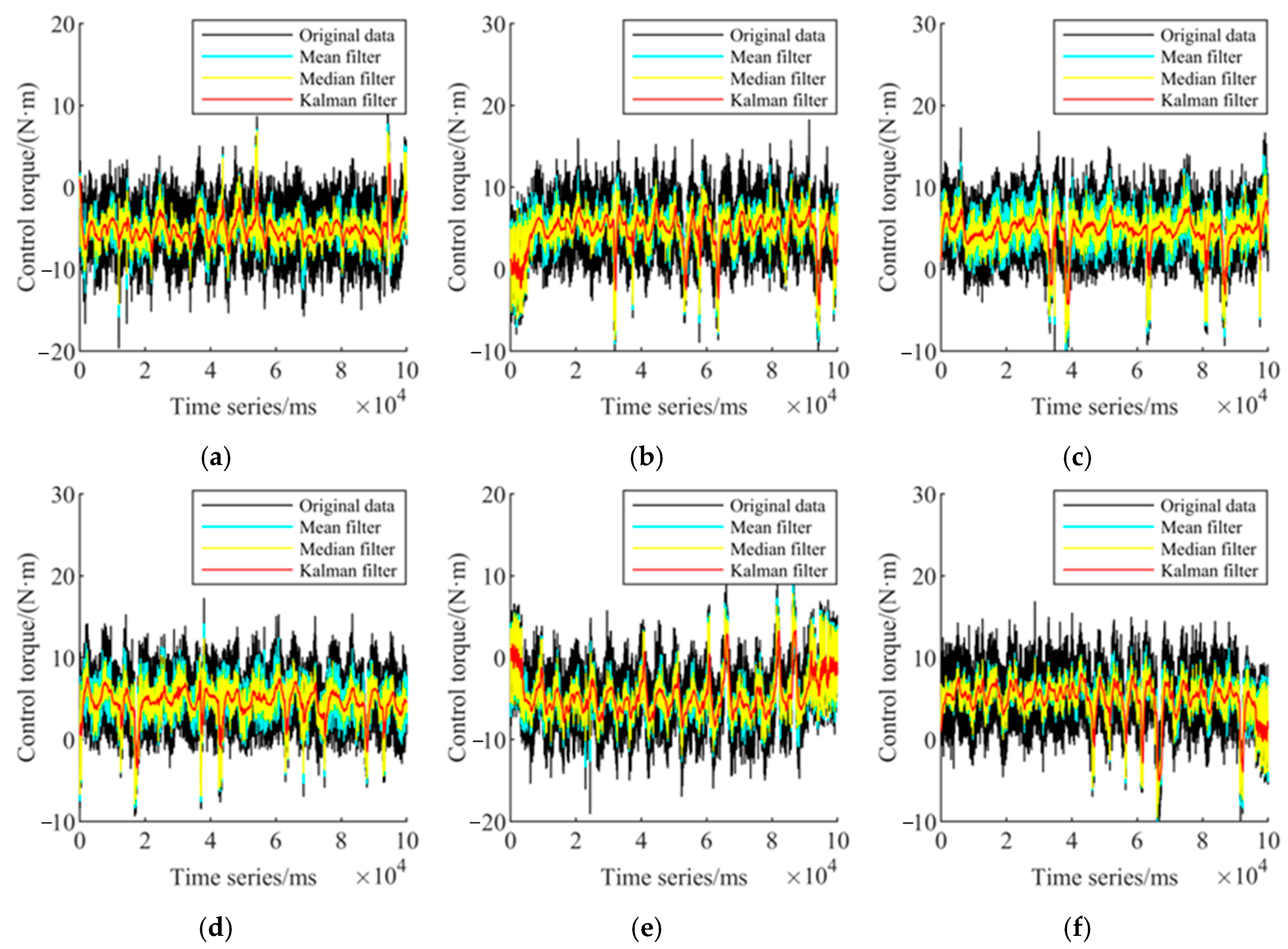
3.2. Performance Evaluation and Analysis of the Extended Kalman Filter

Although Kalman filtering has been widely used in balancing robots, its role is most often associated with state estimation. In contrast, this work focuses on its application to control torque smoothing under real-time balance control constraints. To verify the smoothing effect of the proposed the EKF on the control torques of the LQR balance controller and to mitigate issues such as excessive oscillations and poor convergence caused by large torque fluctuations, the performance of the EKF was evaluated using actual control torque data collected during the robot’s balance control process.

In the experiments, six consecutive time-series data sequences were selected for both the left and right driving wheels, with each sequence spanning 100,000 ms. To further assess the effectiveness of the EKF, two comparative filtering methods—mean filtering and median filtering—were also applied. The resulting performance comparisons for the left and right wheel control torques are shown in Figure 4 and Figure 5, respectively.

As shown in Figure 4 and Figure 5, the raw data exhibit numerous oscillatory spikes, leading to frequent torque jumps under torque control mode and significantly degrading the robot’s real-time control performance. While mean and median filtering can partially attenuate these large spikes, their smoothing capability is limited. In contrast, the EKF provides a markedly superior smoothing effect, effectively reducing spike occurrences and yielding smoother control torques across consecutive time steps.

4. Experiments and Result Analysis

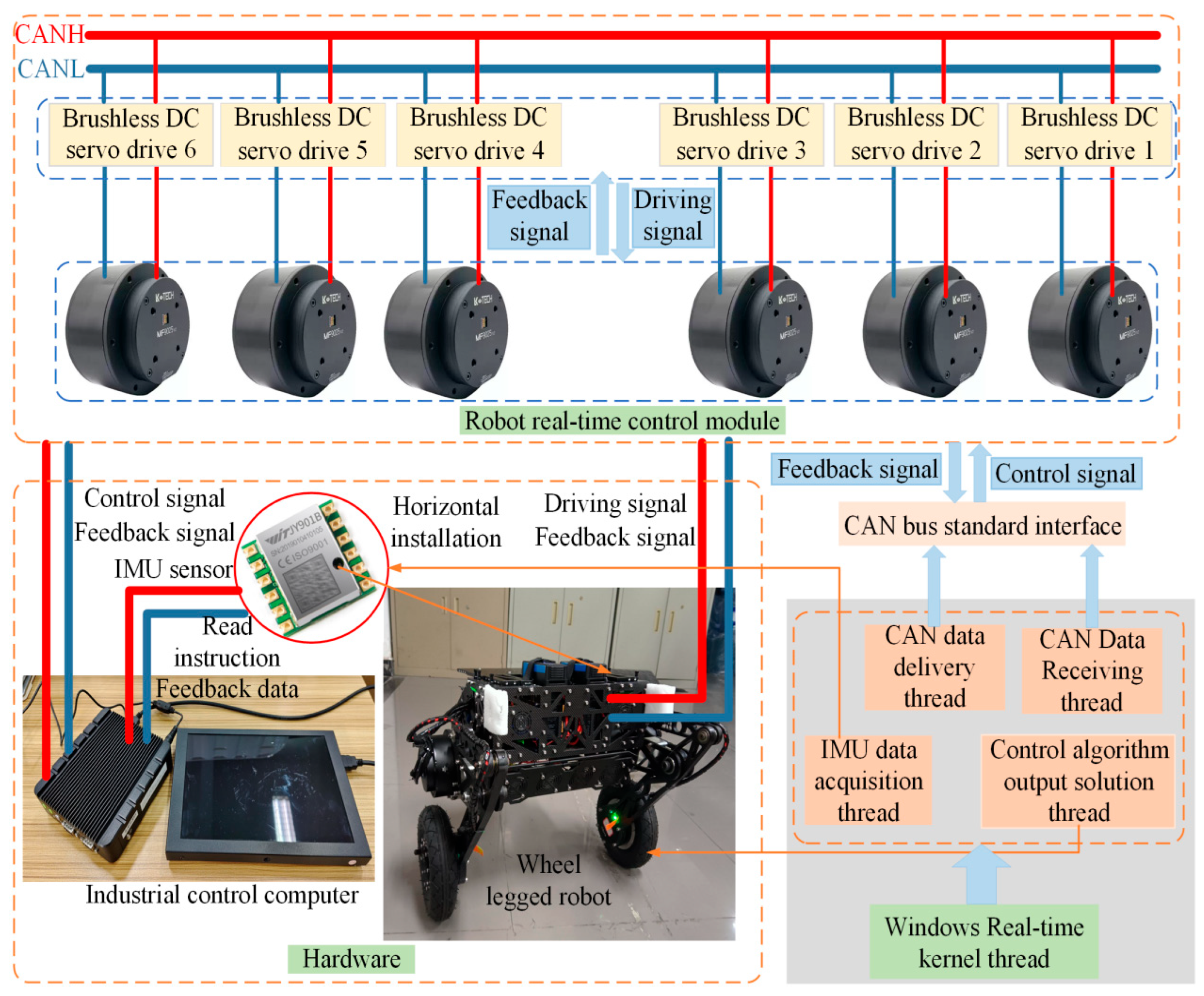
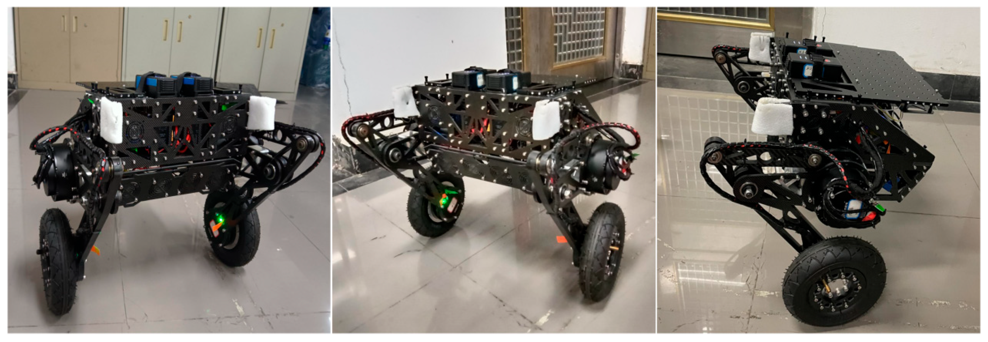
4.1. Balance Control Experiment Platform for the Wheeled Bipedal Robot

To validate the proposed Extended Kalman Filter-based LQR (KLQR) balance control method for the wheeled bipedal robot, a self-designed wheeled bipedal robot and a corresponding balance control experimental platform were developed. A software system was implemented based on the experimental hardware.

The experimental platform primarily comprises the wheeled bipedal robot, an IMU sensor module, an industrial control computer, and a real-time robot control module. The robot is equipped with both wheeled locomotion and leg-based posture adjustment capabilities. The IMU module uses a JY901 nine-axis attitude sensor to acquire the robot’s real-time posture, while the industrial control computer, integrated with the real-time control module, manages the robot’s real-time operations. The detailed configuration of the platform is illustrated in Figure 6.

The real-time control module allocates independent threads for IMU data reception, CAN-protocol motor data handling, and motor control computation, with communication between threads facilitated via global variables. The workflow is as follows: the IMU thread receives and parses sensor data packets, serving as inputs for motor control computation; the motor data reception thread similarly parses CAN messages as additional inputs; the motor control computation thread integrates all state variables to calculate the control input for the current cycle; the motor data transmission thread converts and sends the control input to the motors. The motors execute the control commands to maintain balance, while the real-time system continuously updates the control inputs based on feedback and the algorithm, thereby forming a complete closed-loop control system. The detailed specifications of the motors used in the mechanical system are summarized in

Table 2. The detailed specifications of the motors.

Motor Name	Motor Model	Gear Rate	Max Torque (Nm)	Max Velocity (r/min)
Hip motor	HT8115-J9	9:1	75	57
Knee motor	HT8115-J9	9:1	75	57
Hub motor	MF9025v2		4.9	496

.

4.2. Static Balance Control Experiment and Result Analysis

To validate the proposed KLQR balance control algorithm for the wheeled bipedal robot, the Extended Kalman Filter designed in Section 3 was integrated into the LQR framework to smooth the control torque output, and the controller’s effectiveness was experimentally verified. Each experiment was repeated three times under identical conditions, and consistent performance trends were observed across all trials. For convenience, the LQR controller combined with the filtering algorithm is denoted as KLQR, while the original, unfiltered LQR serves as the baseline for comparison.

To assess whether the proposed algorithm reduces transient fluctuations in the control input and achieves smoother and more stable balance, static balance experiments were conducted on flat ground. To verify repeatability and robustness, three trials were performed. The experimental procedure is illustrated in Figure 7. In each trial, the wheeled bipedal robot operated for approximately 2 min, during which variations in state variables—including displacement, velocity, and pitch angle—were recorded and analyzed.

• Experiment 1

The results of the first static balance experiment are shown in Figure 8. As observed, the pitch angle under the KLQR algorithm remains stable within the range of −0.04 rad to −0.03 rad, with a fluctuation amplitude of only 0.01 rad, corresponding to an estimated RMS value of approximately 0.0035 rad. In contrast, the pitch angle under the LQR algorithm fluctuates between −0.05 rad and −0.02 rad, yielding a fluctuation range of 0.03 rad and an estimated RMS value of about 0.0106 rad, which is approximately three times larger than that of the KLQR algorithm.

In terms of velocity, the KLQR algorithm maintains the speed within ±0.05 m/s, resulting in an estimated RMS velocity of approximately 0.035 m/s. By comparison, the LQR algorithm exhibits a fluctuation range of −0.17 m/s to 0.15 m/s, corresponding to an estimated RMS velocity of about 0.113 m/s—again roughly three times larger than that of KLQR.

Regarding displacement, the KLQR algorithm achieves convergence near 0.01 m with a fluctuation amplitude of ±0.01 m, yielding an estimated RMS displacement of approximately 0.007 m. In contrast, the LQR algorithm shows a wider displacement fluctuation from −0.04 m to 0.1 m, with an estimated RMS value of about 0.050 m, indicating significantly larger position oscillations under LQR control.

2.

Experiment 2

The results of the second static balance experiment are shown in Figure 9. It can be observed that the KLQR algorithm demonstrates consistent performance with that of Experiment 1: the pitch angle stabilizes within −0.04 rad to −0.03 rad with a fluctuation of 0.01 rad, corresponding to an estimated RMS value of approximately 0.0035 rad; the velocity remains within ±0.05 m/s, yielding an estimated RMS velocity of about 0.035 m/s; and the displacement converges at approximately 0.02 m with a fluctuation of ±0.01 m, resulting in an estimated RMS displacement of about 0.007 m.

Although the performance of the LQR algorithm shows slight improvement compared with Experiment 1, it is still inferior to the KLQR algorithm. Specifically, the pitch angle fluctuates from −0.04 rad to −0.01 rad with a fluctuation range of 0.03 rad, corresponding to an estimated RMS value of approximately 0.0106 rad, remaining about three times that of KLQR. The velocity fluctuates from −0.17 m/s to 0.12 m/s, showing a reduced range compared with the previous experiment, but still corresponding to an estimated RMS velocity of about 0.103 m/s, nearly three times larger than KLQR. The displacement fluctuates between −0.05 m and −0.01 m (range of 0.04 m), yielding an estimated RMS displacement of approximately 0.014 m, which is about twice that of the KLQR algorithm.

3.

Experiment 3

The results of the third static balance experiment are presented in Figure 10, showing similar performance trends to those observed in Experiment 2. In particular, the pitch angle under the KLQR algorithm remains confined within a narrow range, corresponding to an estimated RMS value of approximately 0.0035 rad, while the baseline LQR controller exhibits noticeably larger oscillations with an estimated RMS pitch angle of about 0.0106 rad.

Across all three experiments, it is evident that the KLQR algorithm, which incorporates Kalman filtering into the torque output of the baseline LQR controller, is effective. The KLQR algorithm not only maintains the balance of the robot but also significantly reduces convergence oscillations and mitigates shaking behavior around the equilibrium position. Quantitative analysis based on the RMS values of the pitch angle indicates that the oscillatory motion of the robot is reduced by approximately a factor of three compared with the baseline LQR controller.

4.3. Walking and Turning Balance Control Experiments and Result Analysis

The results of the in-place balance experiments indicate that the proposed KLQR algorithm significantly outperforms the LQR algorithm and is more effective for smooth and stable control of the wheeled bipedal robot. To further verify the effectiveness of the KLQR algorithm, uniform linear walking and turning balance experiments were conducted using the KLQR algorithm. Similarly to the in-place balance experiments, to verify the repeatability and stability of the algorithm, three balance experiments were performed for both linear walking and turning scenarios. In each experiment, the wheeled bipedal robot operated for approximately 2 min, and key variables such as displacement, acceleration, and pitch angle were analyzed.

1.

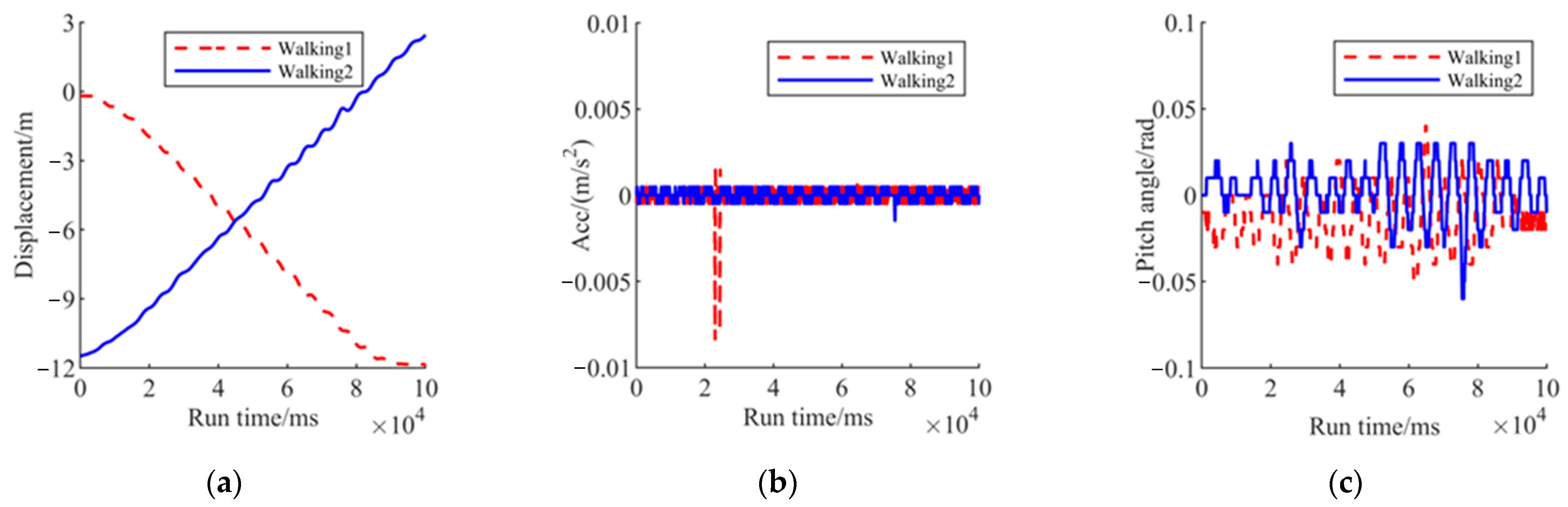
Uniform Linear Walking Balance Experiments

The results of the three uniform linear walking balance experiments are shown in Figure 11, Figure 12 and Figure 13. In Experiment 1, the robot continuously walked forward at a speed of 0.05 m/s; in Experiment 2, it walked forward and then backward at a speed of 0.1 m/s; in Experiment 3, it walked forward at 0.12 m/s and then backward at 0.15 m/s. From the analysis of the results in Figure 11, Figure 12 and Figure 13, it can be seen that in all three experiments, under the control of the KLQR algorithm, the wheeled bipedal robot was able to maintain linear walking with acceleration remaining close to zero, indicating a completely uniform motion state. At the low speed of 0.05 m/s, the pitch angle fluctuations mostly remained within ±0.01 rad, with occasional variations between −0.02 rad and 0.02 rad; at the medium speed of 0.1 m/s, the fluctuations were mostly within ±0.02 rad; at the higher speeds of 0.12 m/s and 0.15 m/s, the pitch angle mostly fluctuated between −0.03 rad and 0.02 rad. As the speed increased, small fluctuations in pitch angle occurred due to factors such as walking resistance and terrain irregularities; however, the robot still maintained excellent stability.

2.

Turning Balance Experiments

The results of the three turning balance experiments are shown in Figure 14, Figure 15 and Figure 16. In Experiment 1, the robot walked forward at a speed of 0.15 m/s and then turned and continued walking forward; in Experiment 2, it walked forward at 0.15 m/s and then turned and walked backward; in Experiment 3, it walked backward at 0.1 m/s and then turned and walked forward. From the analysis of the results in Figure 14, Figure 15 and Figure 16, it can be seen that in all three experiments, under the control of the KLQR algorithm, the wheeled bipedal robot maintained stable linear walking before and after turning, with acceleration remaining close to zero, indicating uniform motion. Meanwhile, the pitch angle fluctuations mostly remained within ±0.03 rad.

The six uniform walking and turning experiments demonstrate that during locomotion control, the KLQR algorithm ensures that the robot remains stable with minimal fluctuation, without noticeable deviations in walking trajectory or sudden acceleration or deceleration. Therefore, applying the Extended Kalman Filter to smooth the control torque effectively eliminates torque spikes and achieves smooth transitions between control inputs over time, which enhances the smoothness performance of the LQR balance controller for the robot.

4.4. Comparison with Existing Methods

Based on the experimental results presented above, this subsection provides a comparison between the proposed KLQR approach and representative balance control methods reported in the literature. Due to differences in robotic platforms, task definitions, and evaluation metrics, the comparison is conducted at a methodological level rather than through direct numerical performance metrics. The comparison focuses on control structure, modeling assumptions, and whether control torque smoothness is explicitly addressed.

Table 3. Comparison with previous studies.

Method	Control Framework	Model Type	Torque Smoothing
LQR-based [37]	Linear feedback	Linearized	NO
MPC-based [16]	Optimization-based	Nonlinear	NO
Robust control [38]	Robust/adaptive	Linear/nonlinear	NO
Ours	LQR + EKF	Linearized	YES

presents a methodological comparison between the proposed KLQR approach and representative balance control methods reported in the literature. LQR-based approaches typically rely on linearized models and focus on stabilizing the robot posture through state-feedback control. While effective for balance regulation, these methods generally do not explicitly address the smoothness of the control torque, which may result in torque spikes when sensor noise or modeling inaccuracies are present.

MPC-based methods formulate balance control as an optimization problem and can incorporate system constraints and predictive behavior. However, their primary objective is trajectory optimization and stability, and control torque continuity is often not explicitly considered. Moreover, the computational complexity of MPC may limit its applicability in high-frequency real-time control scenarios.

In contrast, the proposed KLQR framework explicitly integrates an Extended Kalman Filter into the control loop to smooth the LQR-generated torque output. By modeling the temporal evolution of the control torque and filtering high-frequency fluctuations, the proposed method effectively suppresses torque spikes while preserving balance stability. This distinguishing feature highlights the practical advantage of the KLQR approach for real-world wheeled bipedal robots with actuator and hardware limitations.

5. Conclusions

To address the limitation that conventional wheeled and legged robots cannot simultaneously achieve terrain adaptability and high mobility, a wheeled bipedal robot was designed by integrating the advantages of both locomotion modes. To maintain balance during in-place standing and walking and to reduce the impact of noise on controller robustness, a KLQR balance control algorithm—integrating the EKF with LQR—was proposed to achieve stable balance in both stationary and locomotion scenarios. The conclusions of this study are summarized as follows:

1.

To overcome the trade-off between terrain adaptability and mobility in traditional wheeled and legged robots, a wheeled bipedal robot was developed by leveraging the complementary strengths of legged and wheeled mechanisms. Based on the robot’s dynamic model, an LQR balance control algorithm was constructed to achieve stable balance during in-place standing and walking. Considering the influence of measurement noise and to reduce controller complexity, the EKF was incorporated to smooth the LQR control torque. The resulting KLQR algorithm significantly enhances both the smoothness and robustness of the robot’s motion.

2.

To validate the effectiveness of the proposed KLQR algorithm in reducing noise impact and improving stability, an experimental platform was built using the wheeled bipedal robot, an IMU sensing system, and an industrial PC with a real-time control module. Comparative filtering experiments demonstrated that the integrated EKF effectively suppresses torque spikes. In-place balance tests showed that the KLQR algorithm reduces oscillations by approximately threefold compared with the baseline LQR controller, thereby improving convergence and robustness. Additionally, six experiments involving uniform-speed linear walking and turning at various velocities confirmed that the KLQR algorithm ensures stable locomotion with minimal fluctuation, without noticeable walking deviation or abrupt acceleration and deceleration.

It should be noted that the present study has several limitations regarding the applicability of the proposed method, which also indicate directions for future work. First, the LQR controller is designed based on a linearized dynamic model around the upright equilibrium configuration. Consequently, the effectiveness of the KLQR approach is primarily limited to balance control tasks involving small-to-moderate attitude deviations around this operating point. Extending the proposed framework to handle highly aggressive maneuvers and operating conditions far from the linearization range, for example, by incorporating nonlinear or gain-scheduled control strategies, will be investigated in future studies.

Second, the Extended Kalman Filter in this work is employed to smooth the control torque output rather than to perform state estimation. While this design effectively suppresses high-frequency torque fluctuations and torque spikes, it does not explicitly address severe state estimation errors or large modeling uncertainties. Future work will therefore explore integrating the proposed torque-smoothing mechanism with more advanced state estimation or adaptive modeling techniques to improve robustness under extreme sensor noise and uncertain environments.

Finally, the experimental validation in this study focuses on in-place balancing and constant-speed walking and turning motions on flat ground. The applicability of the proposed method to highly uneven terrain, large external disturbances, and strongly nonlinear dynamic regimes has not been investigated. Future research will aim to extend the KLQR framework to these more challenging scenarios and to validate its performance through more diverse experimental conditions.

References

1. Zhao, Y.; Chai, X.; Gao, F.; Qi, C.K. Obstacle avoidance and motion planning scheme for a hexapod robot Octopus-III. Robot. Auton. Syst. 2018, 103, 199–212. [Google Scholar] [CrossRef]
2. Shi, Q.; Gao, J.; Wang, S.; Quan, X.; Jia, G.; Huang, Q.; Fukuda, T. Development of a Small-Sized Quadruped Robotic Rat Capable of Multimodal Motions. IEEE Trans. Robot. 2022, 38, 3027–3043. [Google Scholar] [CrossRef]
3. Du, W.; Fnadi, M.; Benamar, F. Rolling based locomotion on rough terrain for a wheeled quadruped using centroidal dynamics. Mech. Mach. Theory 2020, 153, 103984. [Google Scholar] [CrossRef]
4. Kim, K.; Spieler, P.; Lupu, E.S.; Ramezani, A.; Chung, S.J. A bipedal walking robot that can fly, slackline, and skateboard. Sci. Robot. 2021, 6, eabf8136. [Google Scholar] [CrossRef]
5. Zhang, Y.; Zhang, L.; Wang, W.; Li, Y.; Zhang, Q. Design and Implementation of a Two-Wheel and Hopping Robot with a Linkage Mechanism. IEEE Access 2018, 6, 42422–42430. [Google Scholar] [CrossRef]
6. Zhu, M.; Zhang, T.; Zou, Y. Imitation-constrained evolutionary learning for multi-locomotion skill of bipedal wheeled robots in unstructured terrains. Eng. Appl. Artif. Intell. 2025, 106, 112079. [Google Scholar] [CrossRef]
7. Yang, J.; Wu, Q.; Li, S.; Ye, Y.; Luo, C. Integrated Modeling and Control Optimization of Biped Wheel-Legged Robot. IEEE Robot. Autom. Lett. 2025, 10, 1465–1472. [Google Scholar] [CrossRef]
8. Miki, T.; Lee, J.; Hwangbo, J.; Wellhausen, L.; Koltun, V.; Hutter, M. Learning robust perceptive locomotion for quadrupedal robots in the wild. Sci. Robot. 2022, 7, eabk2822. [Google Scholar] [CrossRef] [PubMed]
9. Nygaard, T.F.; Martin, C.P.; Torresen, J.; Glette, K.; Howard, D. Real-world embodied AI through a morphologically adaptive quadruped robot. Nat. Mach. Intell. 2021, 3, 410–419. [Google Scholar] [CrossRef]
10. Klemm, V.; Morra, A.; Salzmann, C.; Tschopp, F.; Bodie, K.; Gulich, L.; Küng, N.; Mannhart, D.; Pfister, C.; Vierneisel, M.; et al. Ascento: A Two-Wheeled Jumping Robot. In Proceedings of the IEEE International Conference on Robotics and Automation (ICRA), Montreal, QC, Canada, 20–24 May 2019. [Google Scholar]
11. Zhang, H.; Mohamad Nor, N. Control strategies for two-wheeled self-balancing robotic systems: A comprehensive review. Robotics 2025, 14, 101. [Google Scholar] [CrossRef]
12. Klemm, V.; Morra, A.; Gulich, L.; Mannhart, D.; Rohr, D.; Kamel, M.; Siegwart, R. LQR-assisted whole-body control of a wheeled bipedal robot with kinematic loops. IEEE Robot. Autom. Lett. 2020, 5, 3745–3752. [Google Scholar] [CrossRef]
13. Raza, F.; Owaki, D.; Hayashibe, M. Modeling and Control of a Hybrid Wheeled Legged Robot: Disturbance Analysis. In Proceedings of the IEEE/ASME International Conference on Advanced Intelligent Mechatronics (AIM), Boston, MA, USA, 6–9 July 2020. [Google Scholar]
14. Wang, S.; Cui, L.L.; Zhang, J.F.; Lai, J.; Zhang, D.; Chen, K.; Zheng, Y.; Zhang, Z.; Jiang, Z.P. Balance Control of a Novel Wheel-legged Robot: Design and Experiments. In Proceedings of the IEEE International Conference on and Automation (ICRA), Xi’an, China, 30 May–5 June 2021. [Google Scholar]
15. Zhang, J.; Li, Z.; Wang, S.; Dai, Y.; Zhang, R.; Lai, J.; Hu, J.; Gao, W.; Tang, J.; Zheng, Y. Adaptive optimal output regulation for wheel-legged robot Ollie: A data-driven approach. Front. Neurorobotics 2023, 16, 1102259. [Google Scholar] [CrossRef]
16. Cao, H.X.; Lu, B.; Liu, H.W.; Liu, R.; Guo, X. Modeling and MPC-based balance control for a wheeled bipedal robot. In Proceedings of the 2022 41st Chinese Control Conference (CCC), Hefei, China, 25–27 July 2022; pp. 420–425. [Google Scholar]
17. Kim, S.-K.; Ahn, C.K.; Agarwal, R.K. Observer-Based Proportional-Type Controller for Two-Wheeled Mobile Robots via Simple Coordinate Transformation Technique. IEEE Trans. Veh. Technol. 2021, 70, 11458–11468. [Google Scholar] [CrossRef]
18. Qian, Q.W.; Wu, J.F.; Wang, Z. Dynamic balance control of two-wheeled self-balancing pendulum robot based on adaptive machine learning. Int. J. Wavelets Multiresolution Inf. Process. 2020, 18, 1941002. [Google Scholar] [CrossRef]
19. Xin, Y.X.; Chai, H.; Li, Y.B.; Rong, X.; Li, B.; Li, Y. Speed and Acceleration Control for a Two Wheel-Leg Robot Based on Distributed Dynamic Model and Whole-Body Control. IEEE Access 2019, 7, 180630–180639. [Google Scholar] [CrossRef]
20. Zhao, L.; Yu, Z.; Han, L.; Chen, X.; Qiu, X.; Huang, Q. Compliant Motion Control of Wheel-Legged Humanoid Robot on Rough Terrains. IEEE/ASME Trans. Mechatron. 2024, 29, 1949–1959. [Google Scholar] [CrossRef]
21. Feng, X.; Liu, S.; Yuan, Q.; Xiao, J.; Zhao, D. Research on wheel-legged robot based on LQR and ADRC. Sci. Rep. 2023, 13, 15122. [Google Scholar] [CrossRef]
22. Xu, Y.; Wang, Z.; Lu, C. Design and Control of a Wheeled Bipedal Robot Based on Hybrid Linear Quadratic Regulator and Proportional-Derivative Control. Sensors 2025, 25, 5398. [Google Scholar] [CrossRef] [PubMed]
23. Wang, Y.; Xin, Y.; Rong, X.W.; Li, Y. Whole-body Motion Planning and Control for Underactuated Wheeled-bipdal Robots. In Proceedings of the IEEE International Conference on Robotics and Biomimetics (IEEE ROBIO), Sanya, China, 27–31 December 2021. [Google Scholar]
24. Li, X.; Zhou, H.T.; Feng, H.B.; Zhang, S.; Fu, Y. Design and Experiments of a Novel Hydraulic Wheel-legged Robot (WLR). In Proceedings of the 25th IEEE/RSJ International Conference on Intelligent Robots and Systems (IROS), Madrid, Spain, 1–5 October 2018. [Google Scholar]
25. Cui, L.L.; Wang, S.; Zhang, J.F.; Zhang, D.; Lai, J.; Zheng, Y.; Zhang, Z.; Jiang, Z.P. Learning-Based Balance Control of Wheel-Legged Robots. IEEE Robot. Autom. Lett. 2021, 6, 7667–7674. [Google Scholar] [CrossRef]
26. Xin, Y.X.; Rong, X.; Li, Y.B.; Li, B.; Chai, H. Movements and Balance Control of a Wheel-Leg Robot Based on Uncertainty and Disturbance Estimation Method. IEEE Access 2019, 7, 133265–133273. [Google Scholar] [CrossRef]
27. Khan, J.; Lee, E.; Kim, K. Optimizing the Performance of Kalman Filter and Alpha-Beta Filter Algorithms through Neural Network. In Proceedings of the 2023 9th International Conference on Control, Decision and Information Technologies (CoDIT), Rome, Italy, 3–6 July 2023; pp. 2187–2192. [Google Scholar]
28. Baklouti, S.; Rezgui, T.; Chaouch, A.; Chaker, A.; Mefteh, S.; Sahbani, A.; Bennour, S. IMU Based Serial Manipulator Joint Angle Monitoring: Comparison of Complementary and Double Stage Kalman Filter Data Fusion. In International Conference Design and Modeling of Mechanical Systems; Walha, L., Jarraya, A., Djemal, F., Chouchane, M., Aifaoui, N., Chaari, F., Abdennadher, M., Benamara, A., Haddar, M., Eds.; Lecture Notes in Mechanical Engineering; Springer: Cham, Switzerland, 2023. [Google Scholar]
29. Bai, Y.; Yan, B.; Zhou, C.; Su, T.; Jin, X. State of art on state estimation: Kalman filter driven by machine learning. Annu. Rev. Control. 2023, 56, 100909. [Google Scholar] [CrossRef]
30. Sun, F.; Yu, Z.; Yang, H. A design for two-wheeled self-balancing robot based on Kalman filter and LQR. In Proceedings of the 2014 International Conference on Mechatronics and Control (ICMC), Jinzhou, China, 3–5 July 2014; pp. 612–616. [Google Scholar]
31. Laddach, K.; Łangowski, R.; Zubowicz, T. Estimation of the angular position of a two-wheeled balancing robot using a real IMU with selected filters. Bull. Pol. Acadamy Sci. Tech. Sci. 2022, 70, 1–16. [Google Scholar] [CrossRef]
32. Srichandan, A.; Dhingra, J.; Hota, M.K. An Improved Q-learning Approach with Kalman Filter for Self-balancing Robot Using OpenAI. J. Control. Autom. Electr. Syst. 2021, 32, 1521–1530. [Google Scholar] [CrossRef]
33. Choudhry, O.A.; Wasim, M.; Ali, A.; Choudhry, M.A.; Iqbal, J. Modelling and robust controller design for an underactuated self-balancing robot with uncertain parameter estimation. PLoS ONE 2023, 18, e0285495. [Google Scholar] [CrossRef] [PubMed]
34. Herrera, M.; Benítez, D.S.; Aguirre, O.; Camacho, O. Experimental Validation of Fuzzy-Optimal Control for a Two-Wheeled Inverted Pendulum. In Proceedings of the 2023 IEEE Seventh Ecuador Technical Chapters Meeting (ECTM), Ambato, Ecuador, 10–13 October 2023; pp. 1–6. [Google Scholar]
35. Irfan, S.; Zhao, L.; Ullah, S.; Mehmood, A.; Fasih Uddin Butt, M. Control strategies for inverted pendulum: A comparative analysis of linear, nonlinear, and artificial intelligence approaches. PLoS ONE 2024, 19, e0298093. [Google Scholar] [CrossRef]
36. Cui, Z.; Dai, J.; Sun, J.; Li, D.; Wang, L.; Wang, K. Hybrid Methods Using Neural Network and Kalman Filter for the State of Charge Estimation of Lithium-Ion Battery. Math. Probl. Eng. 2022, 2022, 9616124. [Google Scholar] [CrossRef]
37. Zhang, A.; Zhou, R.; Zhang, T.; Zheng, J.; Chen, S. Balance Control Method for Bipedal Wheel-Legged Robots Based on Friction Feedforward Linear Quadratic Regulator. Sensors 2025, 25, 1056. [Google Scholar] [CrossRef] [PubMed]
38. Zhang, T.; Li, D.; Zou, Y. A robust balance controller of a two-wheeled legged robot based on adaptive neuro-fuzzy inference system. J. Braz. Soc. Mech. Sci. Eng. 2025, 47, 665. [Google Scholar] [CrossRef]
Figure 1. Overall Control Architecture of the Wheeled Bipedal Robot.
Machines 14 00077 g001
Figure 2. Force Analysis of Each Component and State of the Robot (a) Force Analysis of the Left Driving Wheel; (b) Force Analysis of the Chassis; (c) Force Analysis of the Robot during Turning.
Machines 14 00077 g002
Figure 3. LQR Full-State Feedback Controller.
Machines 14 00077 g003
Figure 4. Performance Comparison of Left Wheel Control Torque Filtered by EKF and Other Methods (a) Data sequence 1; (b) Data sequence 2; (c) Data sequence 3; (d) Data sequence 4; (e) Data sequence 5; (f) Data sequence 6.
Machines 14 00077 g004
Figure 5. Performance Comparison of Right Wheel Control Torque Filtered by EKF and Other Methods (a) Data sequence 1; (b) Data sequence 2; (c) Data sequence 3; (d) Data sequence 4; (e) Data sequence 5; (f) Data sequence 6.
Machines 14 00077 g005
Figure 6. Experimental platform of the wheeled bipedal robot for balance control.
Machines 14 00077 g006
Figure 7. Process of Static Balance Experiment on Flat Ground.
Machines 14 00077 g007
Figure 8. Results of Static Balance Experiment 1 on Flat Ground (a) Displacement; (b) Velocity; (c) Pitch Angle.
Machines 14 00077 g008
Figure 9. Results of Static Balance Experiment 2 on Flat Ground (a) Displacement; (b) Velocity; (c) Pitch Angle.
Machines 14 00077 g009
Figure 10. Results of static balance experiment 3 on flat ground (a) Displacement; (b) Velocity; (c) Pitch Angle.
Machines 14 00077 g010
Figure 11. Results of walking balance experiment 1 (a) Displacement; (b) Acceleration; (c) Pitch Angle.
Machines 14 00077 g011
Figure 12. Results of walking balance experiment 2 (a) Displacement; (b) Acceleration; (c) Pitch Angle.
Machines 14 00077 g012
Figure 13. Results of walking balance experiment 3 (a) Displacement; (b) Acceleration; (c) Pitch Angle.
Machines 14 00077 g013
Figure 14. Results of turning balance experiment 1 (a) Displacement; (b) Acceleration; (c) Pitch Angle.
Machines 14 00077 g014
Figure 15. Results of turning balance experiment 2 (a) Displacement; (b) Acceleration; (c) Pitch Angle.
Machines 14 00077 g015
Figure 16. Results of turning balance experiment 3 (a) Displacement; (b) Acceleration; (c) Pitch Angle.
Machines 14 00077 g016