Abstract
Savonius drag-based rotors, a type of vertical-axis wind turbine (VAWT), are well-suited for urban environments—particularly residential rooftops—owing to their compact design and ability to capture wind from all directions. However, their relatively low efficiency and narrow operational range pose significant challenges, such as limited energy output under variable wind conditions and reduced performance across a broad range of tip speed ratios. To address these issues, this study explores flow augmentation using strategically placed deflectors, referred to as Wind Accelerators and Guiding Rotor Houses (WAG-RHs). Four different configurations, including double, triple, oblique, and straight designs, were evaluated against both omni-directional guide vanes (ODGVs) and a conventional rotor. The findings show that the ODGV configuration successfully extends the operational range from a tip speed ratio of 0.5 to 0.6—termed the extended performance point (EPP)—and increases the power coefficient () by up to 300% compared to the conventional design. Among all setups, the straight WAG-RH configuration proved most effective, not only achieving the EPP but also delivering a 385% and 264.3% increase in local and AVE values, respectively compared to the conventional rotor. It also outperformed the ODGV-equipped rotor by 25%, thanks to its radial and dual-plane arrangement.
1. Introduction
The recent surge in air pollution and carbon emissions from fossil fuel consumption has accelerated the development of renewable energy sources such as solar [1], wind [2], and biomass [3]. Among these, wind energy stands out as a reliable, widely accessible, and cost-effective option, making it a strong candidate for promoting clean energy adoption [2]. Wind turbines are the core technology in wind energy systems, designed to convert kinetic wind energy into electrical power. They are typically classified by their axis of rotation into horizontal-axis wind turbines (HAWTs) [4] and vertical-axis wind turbines (VAWTs) [5]. VAWTs, with their omnidirectional operation and low maintenance requirements, have recently emerged as a reliable solution for urban wind power applications, especially for rooftop installations on buildings [6]. They can be categorized based on the aerodynamic forces driving their rotation. The first type, lift-based VAWTs, operate using lift forces generated by pressure differences between the inner and outer sides of the blades. This category includes conventional H-type Darrieus VAWTs [7] and helical Darrieus VAWTs, also known as Gorlov VAWTs [8]. These turbines operate efficiently at high tip speed ratios (TSRs) and provide higher power output. However, they suffer from reduced torque at low TSRs, leading to poor self-starting capability—an important limitation for rooftop applications, where wind speeds are generally lower [9]. In contrast, drag-based VAWTs, such as Savonius VAWTs [10], operate based on the drag forces generated by pressure differences between the convex and concave sides of the turbine buckets. These wind turbines function effectively in low-speed environments and at low TSRs, offering reliable self-starting performance. While their power coefficient () decreases at higher TSRs due to their low-speed design, their simplicity, stability, and consistent start-up capability make them well-suited for urban and rooftop installations [11].
Given the relatively low efficiency of Savonius VAWTs compared to lift-based rotors, there is increasing interest in enhancing their performance and expanding their operational range. Key enhancement strategies include modifying the rotor blade geometry and integrating external flow augmentation devices to better direct airflow toward the buckets [12]. Among blade modification approaches, Tahani et al. [13] demonstrated that helical Savonius VAWTs outperform conventional designs, as their bucket geometry enhances pressure differentials around the convex and concave sections, improving flow discharge. Similarly, Lajnef et al. [14] reported that delta-shaped bucket designs increased the by 29.5% over standard helical rotors. Nasef et al. [15] demonstrated that adding a flipper to the bucket can improve the by 38.5% compared to the conventional Savonius rotor. In contrast, using a dual pair of buckets offers a 28.5% increase in . A scooplet-based design—with non-overlapping main buckets and curved secondary buckets matching the primary shape—achieved a enhancement of up to 39% [16]. Al-Ghriybah et al. [17] demonstrated that adding a wavy pattern to the concave side of the bucket can improve efficiency by up to 14.5% compared to conventional designs. Building on this, Al-Gburi et al. [18] showed that optimizing the wave depth and height further increases the by up to 22.8%. Similarly, Harsito et al. [19] found that a 5 mm slotted bucket enhanced the by 16%, whereas a 9 mm slot resulted in reduced performance compared to the conventional rotor.
In addition to blade-modification methods, the integration of external components—such as flow augmenters—offers a promising strategy for enhancing performance. These devices can be strategically positioned around the rotor within the rotor housing (RH), including configurations like semi-directional guide vanes [20] and omni-directional guide vanes (ODGVs) [21]. Alternatively, they can be positioned in adjacent areas outside the RH, such as a subsonic convergent nozzle [22], offering additional opportunities for performance optimization. As Savonius rotors are significantly affected by the negative torque generated by the returning bucket, various augmentation techniques have been implemented to mitigate this effect and enhance the overall operational performance of the turbine [23]. Deflector systems, placed either inside or outside the RH, have been widely used in numerous studies focused on augmentation. Their primary objective is to divert incoming wind away from the returning bucket and direct it toward the concave surface of the advancing bucket, thereby increasing the pressure differential between the concave and convex sides [24]. When guide vanes or plate shields are arranged in an optimized configuration, they can significantly enhance the , with reported values exceeding 0.5 [25]. Layeghmand et al. [26] demonstrated that installing an airfoil-shaped guide vane (GV) outside the RH can increase the by up to 50% compared to the conventional Savonius VAWT. This airfoil-inspired GV, when optimally positioned, effectively delays flow separation on its upper surface, offering superior performance over flat plate deflectors and conventional GVs. In contrast, a simple plate deflector achieved only a 27% improvement in the [27]. More recently, Salleh et al. [28] demonstrated that incorporating double flat plate deflectors within the RH—tuned to optimal lengths and angles—can enhance the by approximately 66% to 171% compared to baseline rotor configurations.
The most appropriate flow augmentation method for VAWTs in urban environments, particularly on rooftop installations, is the use of flat plate deflectors and GVs within the RH. These configurations, often referred to as ODGV systems, employ multiple flat plate deflectors or GVs arranged at various angles within the RH to regulate airflow and reduce the negative torque acting on the returning bucket [29]. One such ODGV system, featuring eight flat plates positioned at a 20° installation angle, achieved a 28% increase in the by enhancing flow control and mitigating counterproductive torque [30]. Building on the ODGV concept, Manganhar et al. [31] introduced a flow-augmentation system consisting of deflectors positioned at 45° around the rotor. This configuration, termed the Wind Accelerator and Guiding Rotor House (WAG-RH), significantly improved aerodynamic performance, resulting in a 75% increase in the compared to the conventional rotor.
According to the literature, drag-based Savonius VAWTs are suitable for urban applications, particularly for residential settings where they can be installed on building rooftops. However, their low and narrow operational range present significant limitations, necessitating the use of flow-augmentation methods to improve performance. Previous studies have largely focused on enhancing airflow through the use of external components near the rotor at the RH with ODGV configurations or simple deflector setups. However, the optimum deflector arrangement in the form of a WAG-RG remains an open research question. This study addresses this gap by systematically investigating the most effective deflector configurations within the RH on both suction and discharge sections of the rotor, referred to as the WAG-RH. The analysis focuses on evaluating turbine performance and airflow behavior both around the rotor and in the surrounding flow field. To the best of our knowledge, this research represents the first comprehensive effort to identify the strategic position of the deflectors, which refers to the optimal arrangement of deflectors as part of the WAG-RH. Previous studies primarily focused on ODGV or basic deflector configurations. However, the current research offers a detailed analysis of performance metrics in conjunction with flow physics, providing in-depth insights into the most effective positioning of deflectors. The significance of this research lies in its objective to optimize efficiency in rooftop installations while enhancing energy harvesting within urban settings.
2. Model Setup
In the current CFD simulation, a Savonius VAWT rotor based on the design characterized by Wenehenubun et al. [32] was utilized. The geometric specifications of the turbine under investigation are presented in Table 1.

Table 1.
Savonius rotor dimensions [32].
In this simulation, deflectors are strategically arranged, which refers to the appropriate and optimized placement of deflectors around the rotor on both suction and discharge sections, aiming to enhance flow guidance and aerodynamic performance within the RH domain as part of the WAG-RH system to effectively direct airflow toward the rotor. This study examines several deflector configurations, including double, triple, oblique, and straight deflector arrangements—as illustrated in Figure 1.
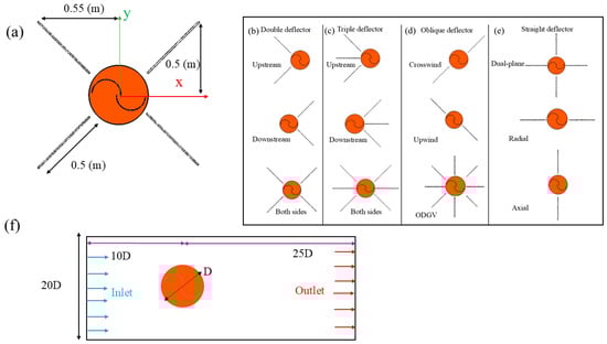
Figure 1.
(a) Rotor with sample deflector; (b–e) rotor with various WAG-RH configurations, (f) conventional rotor and domain setup.
According to Figure 1, deflectors are strategically positioned around the rotor within the RH domain. Each deflector measures 0.5 m in length, with horizontal and vertical extensions of 0.55 m and 0.5 m, respectively, from the rotor center. Four primary WAG-RH configurations are examined: double deflectors, triple deflectors, oblique deflectors, and straight deflectors, along with the ODGV configuration. In double and triple configurations, when the deflectors are positioned on the rotor’s suction side, this arrangement is referred to as the “upstream” configuration. Conversely, when the deflectors are situated on the rotor’s discharge side, it is termed the “downstream” configuration. Additionally, when deflectors are installed on both the suction and discharge sides, this is identified as the “both-side” arrangement. In the context of oblique deflectors, the configuration is referred to as “crosswind” when positioned to face the direction of the prevailing wind. Conversely, when the deflectors are oriented upwards, they are designated as “upwind”. In a straight configuration, deflectors installed vertically and horizontally are referred to as “axial” and “radial”, respectively. When deflectors are positioned in both directions, they are termed “dual-plane”. These configurations are evaluated against both the conventional rotor and the rotor equipped with the ODGV-based WAG-RH system.
3. Governing Equations and Numerical Setup
This section discusses the governing equations underlying the current simulation, along with the numerical setup implemented in the CFD solver.
3.1. Fluid Mechanics Equations
To analyze the complex flow dynamics around turbine buckets or blades, the Unsteady Reynolds-Averaged Navier–Stokes (URANS) equations are utilized, as this approach is highly effective for simulating the VAWT flow field due to its capacity to accurately capture unsteady flow phenomena, such as blade rotation and wake interactions, while effectively managing computational cost and accuracy. This method facilitates the resolution of time-dependent flow separation and vortex shedding, which are critical for accurately predicting rotor performance. URANS, an extension of the Reynolds-Averaged Navier–Stokes (RANS) equation, includes time-dependent terms to more accurately capture transient flow behavior. These equations describe the interaction between pressure and velocity fields using time-averaging methods to evaluate turbulence. Grounded in Newton’s laws of motion, they also satisfy the principles of momentum and mass conservation. The URANS formulation is given as follows [33]:
The terms and represent the mean velocity components in a Cartesian coordinate system, reflecting the principles of fluid flow dynamics. Additionally, the fluctuating velocities and capture the influence of the turbulence in the flow. , and denote the mean pressure, fluid density, and kinematic viscosity, respectively. The term represents the Reynolds stress tensor, which quantifies the correlation between fluctuating velocity components. This tensor provides critical insight into the momentum transfer and turbulence-induced stresses by the fluid flow.
3.2. Turbulence Modeling Equations
The impact of Reynolds stress on fluid flow requires the careful selection of a turbulence model to ensure accurate simulation around blades and buckets. Commonly used models include the and models, both of which solve two transport equations. The model employs empirical damping functions within the viscous sub-layer but tends to be less accurate under adverse pressure gradients, making it less suitable for turbomachinery CFD simulations. In contrast, the model provides greater accuracy near wall surfaces but is sensitive to turbulence conditions such as turbulence intensity. To overcome these limitations, the shear-stress transport (SST) model was developed, combining the model in regions away from rotor walls with the model near the rotor walls, thereby improving overall accuracy [34]. Previous CFD studies on VAWTs indicate that the SST turbulence model is the most accurate option among RANS-based models for simulating turbulent flow around VAWT blades or buckets. It provides more precise results compared to the one-equation Spalart–Allmaras model, which is better suited for low-Reynolds-number flows, as well as the standard two-equation models like and . The SST model effectively captures velocity fluctuations near the blades and accurately represents velocity development in far-field regions [35,36]. Based on this evidence, the SST model is employed in the current simulation. Here, turbulent kinetic energy represents the energy contained in turbulent eddies and vortices, while the specific dissipation rate quantifies the rate at which this energy dissipates due to viscous effects. The governing equations for and are presented below [37].
where and represent the dissipation and generation of turbulent kinetic energy, respectively. Similarly, and denote the generation and dissipation of specific dissipation rate ω, respectively. The turbulent Prandtl numbers for and are denoted by and , respectively. Turbulent viscosity is computed based on the values of and .
3.3. Turbine Mathematical Relations
Rotor performance is evaluated using the torque coefficient ( and power coefficient , which are defined as follows [38]:
where represents the rotor output power, is the air density (taken as 1.225 ), and is the normal wind velocity. The swept area () is calculated as the product of rotor diameter () and height (; in this 2D simulation, is set to 1. The tip speed ratio (TSR) is a crucial dimensionless design parameter, defined as the ratio of the tangential velocity at the bucket tip to the normal wind velocity [38]:
where is the angular velocity of the rotor and is the rotor radius.
3.4. Computational Domain
This study employed a 2D CFD approach to analyze the flow dynamics around Savonius rotor buckets and the downstream wake development. The 2D method was chosen for its effectiveness in accurately capturing wake behavior at the rotor midplane and simulating tip vortices, while offering reduced computational costs [39]. A sensitivity analysis was performed on three key geometrical parameters to ensure consistent upstream and downstream flow behavior and to minimize the influence of the side walls on rotor performance and flow characteristics. The parameters examined include the following: (a) , the distance from the rotor center to the inlet, ranging from to ; (b) , the distance from the rotor center to the outlet, ranging from to ; and (c) the blockage ratio (), where represents the width of the computational domain. The results of this sensitivity analysis are presented in Figure 2.
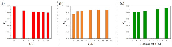
Figure 2.
Computational domain sensitivity analysis: (a) effect of inlet distance, (b) effect of outlet distance, and (c) effect of domain width.
As shown in Figure 2a, inlet distances of and tend to overestimate the power coefficient . The difference in between and is minimal, with a deviation of less than 1%. Therefore, selecting is a suitable and efficient choice, as it ensures accurate results without overestimating while also allowing for proper upstream flow development without reverse flow. In Figure 2b, it is evident that as the outlet distance increases from to , the variation in becomes progressively smaller, with a maximum deviation of only 0.2% within this range. Based on this analysis, is recommended as the optimal outlet distance. Figure 2c indicates that a blockage ratio of 10% leads to an overestimation of due to side-wall-induced flow acceleration. To improve accuracy, a domain width of , corresponding to a blockage ratio of 5%, has been adopted. In summary, to ensure fully developed downstream flow, the outlet was positioned 25 rotor diameters away from the rotor. Similarly, the inlet was placed 10 rotor diameters upstream to maintain uniform inflow and avoid upstream interference.
3.5. Boundary Conditions and Solver Setup
This simulation is based on the assumption of a uniform inlet wind velocity of 10 m/s. At the outlet boundary, a static gauge pressure of zero is applied to represent far-field outflow conditions accurately. In addition, the lateral boundaries are positioned sufficiently far from the rotor to minimize their impact on the flow field; thus, symmetry boundary conditions are applied to these sides. A non-slip condition is imposed on the turbine walls, which also rotate with the angular velocity defined for the rotating domain. To accurately model the interaction between the rotating and stationary regions, an interface condition is employed between the rotor and the surrounding stationary domain. The rotation of the rotor is represented using a mesh motion technique. Therefore, the interface between the rotor and the stationary zone becomes coupled, and the angular velocity applied to the rotor results in the rotation of this coupled interface, consistent with the sliding mesh interface methodology. In accordance with experimental data obtained from low-speed wind tunnel testing under low turbulence intensity (TI), the turbulence intensity is set to 1% at both the inlet and outlet boundaries.
The simulation was conducted using the Ansys Fluent 2021 R1 software package. Due to the unsteady nature of the flow around the rotor buckets and the time-dependent behavior observed in recent numerical studies, a transient analysis approach was adopted. Given that air is treated as an incompressible fluid, a pressure-based solver was selected to resolve the continuity and momentum equations. The SIMPLE scheme was employed for velocity–pressure coupling, while second-order discretization was applied to enhance solution accuracy. For solution convergence, residual thresholds were set to for the continuity, x-velocity, y-velocity, turbulent kinetic energy (k), and specific dissipation rate (ω) equations. To meet these criteria, 30 iterations were performed per time step. The convergence behavior was further assessed by monitoring , ensuring that torque and power fluctuations followed a consistent and repeatable trend before considering any rotor cycle as valid. The power coefficient was computed only after verifying the stabilization of torque oscillations. Thus, a rotor cycle was deemed acceptable for the performance evaluation only after confirming convergence in both residuals and output trends.
3.6. Grid Study
Achieving accurate and reliable CFD results depends heavily on high-quality mesh generation and the appropriate application of boundary conditions. To this end, strict meshing standards were maintained throughout the process to ensure the accuracy and reliability of the simulation results. In this research, Ansys Mesh was utilized to generate an unstructured grid for both the rotor and stationary zones. Unstructured grids are widely used in CFD simulations due to their ability to represent complex geometries with high accuracy. To reduce numerical errors and ensure solution fidelity, a fine mesh of 4 mm was applied at the rotor–stator interface, effectively minimizing abrupt transitions between the rotor and stationary zones. Mesh quality around the buckets is critically important for accurately capturing flow dynamics, especially near the bucket tips where velocity gradients are high. Accordingly, a refined mesh was applied in these zones, along with boundary layer meshing, to enhance the precision of the simulation further. This meshing approach enables a gradual transition in the size of polyhedral triangular grids, effectively approximating the characteristics of prism layers. It is derived from the boundary layer grid, which incorporates inflation layers around the buckets to enhance mesh quality and simulation accuracy. This method successfully addresses sudden changes in grid size by ensuring seamless integration between the boundary layer prism mesh surrounding the buckets and the adjacent triangular grid associated with the rotor. Furthermore, the apex of each triangular element is precisely aligned with the prism layer edges, maintaining mesh continuity. A sliding interface was implemented using a non-conformal mesh with carefully defined element sizing, designed to increase grid density and improve the accuracy of flux calculations across the interface. The resulting grid structure is illustrated in Figure 3.
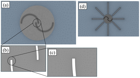
Figure 3.
Grid generation for the following: (a) rotor and stator zones, (b) bucket tips, (c) zoomed-in view of a bucket tip, (d) rotor with WAG-RH configuration (omnidirectional case).
As illustrated in Figure 3, a denser grid network is observed around the bucket tips, with a gradual coarsening of the mesh toward the rotor–stator interface. Similarly, in the rotor equipped with a WAG-RH in an omnidirectional configuration, increased mesh density is evident around the GVs. The grid network specifications for four distinct mesh levels—developed for grid independence and sensitivity analysis—are detailed in Table 2. The necessity of developing a grid network at different levels is to ensure that the simulation results are independent of the mesh and to verify grid convergence. In this study, grid level 1 corresponds to the coarsest mesh, while grid level 4 represents the finest mesh.
Table 2.
Grid independence study summary.
Specific ranges of the dimensionless wall distance are utilized to identify the viscous sublayer and the buffer layer within the turbulent boundary layer. Typically, the viscous sublayer falls within the range 0 5, while the buffer layer spans 5 30. To ensure accurate simulation results when using the SST turbulence model, it is crucial to maintain values below 1, indicating a high-quality near-wall mesh. The value can be calculated using the following equation [40,41]:
where represents the normal distance between the grid center and the bucket wall, and are the density and dynamic viscosity of the fluid at the wall, respectively, and is the friction velocity. The friction velocity is defined as , where is the wall shear stress, calculated as . Figure 4 shows the distribution of around the bucket surfaces, confirming that the mesh meets the near-wall resolution criteria required for the SST model.
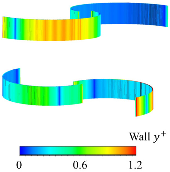
Figure 4.
Spanwise distribution and contour plot of wall on the bucket surface.
According to Figure 4, the maximum values are observed at the bucket tips, reaching approximately 1, which falls within the acceptable range for the SST turbulence model. The concave sides of the buckets exhibit near-zero values, while the convex sides present slightly elevated values, around 0.5. Overall, the distribution of remains within acceptable limits across the bucket surfaces, indicating a high-quality near-wall mesh. Another important grid quality metric is skewness, which must remain below 1 in triangular grid structures to ensure numerical stability and avoid divergence issues [42]. As shown in Table 1 and Figure 4, both and skewness metrics are within acceptable thresholds, confirming the adequacy of the mesh. Additionally, the analysis of various grid levels reveals no significant discrepancies in the AVE and values. Specifically, the differences in AVE between grid level 2 and grid levels 1, 3, and 4 are observed to be 2%, 0.5%, and 0.2%, respectively. Given that the differences in AVE values between grid level 2 and finer grids are below 1%, grid level 2 is deemed sufficient for accurate simulation. This indicates that the CFD solution is independent of the grid density and size and that the governing of fluid dynamic behavior primarily drives the simulation results. A detailed evaluation of the torque profile over a full rotor revolution is essential for a robust grid independence assessment. Figure 5 illustrates the torque coefficient variation over one full cycle for all grid levels.
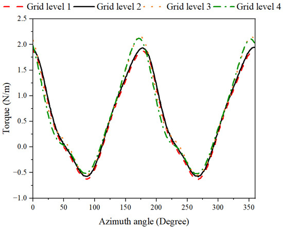
Figure 5.
Rotor torque as a function of the azimuth angle during a complete rotation at TSR = 0.37.
According to Figure 5, the rotor torque fluctuations over a complete rotation are nearly identical across the various grid levels. The most notable deviation occurs between grid levels 4 and 2 at an azimuth angle of 175°, where an 8% variation is observed. This discrepancy remains within acceptable limits and supports the conclusion of grid convergence. Given the convergence behavior and the consistent torque trends across different grid levels, grid level 2 has been selected for this simulation. This choice balances accuracy and computational efficiency, as employing a finer mesh would significantly increase computational costs without yielding proportionate improvements in the results.
3.7. Time Step Size Study
Temporal and spatial discretization play a critical role in CFD simulations, particularly due to the unsteady flow behavior near the bucket walls and the presence of significant velocity gradients. Therefore, conducting a time-step sensitivity study is crucial for accurately capturing these complex flow phenomena [43]. Proper discretization not only ensures the precision of the simulation results but also contributes to the stability of the numerical solution. The Courant–Friedrichs–Lewy (CFL) criterion serves as a fundamental guideline in numerical analysis for selecting appropriate time-step sizes in relation to the spatial resolution of the mesh. The formulation of the Courant number is provided in Equation (8) [44].
where u represents the velocity captured within the bucket, denotes the time-step size, and signifies the average distance between two adjacent cell centroids along the bucket wall. The Courant number quantifies the relationship between the temporal time step and the time required for a fluid particle, traveling at a velocity , to traverse a cell of characteristic length . In viscous turbomachinery flow simulations, maintaining a Courant number close to 10 is generally considered optimal for minimizing computational errors and ensuring solution stability [44]. Also, Equation (10) expresses the relationship between the time step and the rotor’s azimuth angle for varying angular velocities.
The calculation defines the relationship between the time-step size and azimuth angle, where denotes the variation in azimuth angle due to rotor rotation, and Ω represents the angular velocity. Table 3 presents the Courant number values for various grid levels and time steps, corresponding to different values of and at a TSR of 0.37. The differences in time-step values result from specific assignments for each angular velocity, as defined in Equation (10). These variations are expected to have a negligible effect on output parameters, such as . Furthermore, since the CFL condition remains within an acceptable range, simulation can be considered time-step-independent, allowing for the selection of an optimal time step that balances accuracy and computational efficiency.
Table 3.
CFL for various spatial and temporal discretization schemes.
According to Table 3, for or , the CFL number remains within an acceptable range for grid levels 1 and 2. Based on this observation and in view of the grid study results—which demonstrated that grid level 2, with its finer mesh resolution, provides suitable accuracy—it is recommended that grid level 2 with a time-step size of 0.0005 (s) be selected for the remainder of the simulations. To further verify the robustness of the results and confirm their independence from the chosen time-step size, an additional analysis was conducted alongside the CFL number assessment. In this analysis, the coefficient was evaluated at various time-step sizes, as summarized in Table 3, and plotted as a function of the azimuth angle. The corresponding results are presented in Figure 6.
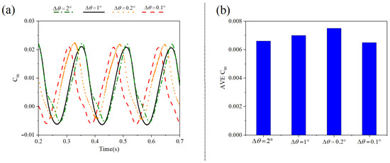
Figure 6.
(a) Variation of over time for different time-step sizes, and (b) time-step sensitivity analysis.
According to the analysis presented in Figure 6, the variations in exhibit a consistent pattern throughout all examined time-step sizes. Notably, the peaks in become more closely spaced as the time step is reduced. Additionally, fluctuations in the values have been observed for , which is commonly encountered in numerical modeling when utilizing very fine time steps. Furthermore, the time-step sensitivity analysis shows that the averaged values for different time steps are in close agreement. The averaged value at (corresponding to ) was selected for the current modeling, despite a 6% deviation from the average at . This deviation is considered minor, and the chosen value is regarded as the most suitable for the requirements of the study. Overall, these findings confirm that the solution is effectively independent of the time-step size and that the chosen discretization does not influence the underlying physics of the flow.
Following the grid-independence study, it was determined that variations in were negligible from grid level 2 onwards. As a result, grid level 2 was selected for use in the discretization process. The simulation time step was set based on (equivalent to which yields a CFL number of approximately 10 for grid level 2. Therefore, this combination of the grid network and time-step size was adopted for the solution discretization.
3.8. CFD Model Validation
Validation of the CFD model is a crucial step in ensuring the reliability of numerical simulations. In this study, validation was performed by comparing the simulation results with the experimental data of Wenehenubun et al. [32]. Since the experimental setup did not account for the blocking effect, this factor was also excluded from the CFD simulations to maintain consistency. In the reference study conducted by Wenehenubun et al. [32], the wind tunnel velocity was established within the range of 1 to 10 m/s, with a specific selection of 6 m/s for evaluating the performance of a two-bladed Savonius VAWT. This experimental investigation included TSR ranges from 0 to 0.51; however, validation of the results was confined to the range of 0.4 to 0.51 and adhered to the selected free wind velocity of 6 m/s. The validation results are presented in Figure 7. Furthermore, Table 4 delineates the Absolute Percentage Error (APE), the Mean Absolute Percentage Error (MAPE), and the Root Mean Square Error (RMSE).
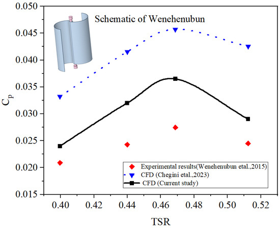
Figure 7.
Comparison of from the present 2D simulation with experimental data and previous CFD results [32,45,46].
Table 4.
Statistical data of validation.
Based on Figure 7, the current CFD results closely align with the experimental data, showing the peak occurring at a TSR of 0.469 or an ω of 25.4 rad/s. Following this TSR, the values declined in accordance with the Betz limit. Also, according to Table 4, the APE between the current CFD model and the experimental results occurs at a TSR of 0.47, yielding a discrepancy of 33.3%. For comparative purposes, the CFD findings reported by Chegini et al. [45], which were derived under similar boundary conditions and configurations, exhibit a comparable trend with the experimental data. However, their results demonstrate a greater APE across all TSR ranges. Notably, at TSR = 0.4, their simulation deviates from the experimental values by more than 58%, in contrast to the current CFD model, which reflects only a 14.8% deviation. Furthermore, the previous CFD model exhibited significant inaccuracies, with an MAPE of approximately 67.6% and an RMSE of 0.01665. In contrast, the current CFD model demonstrates significantly improved alignment with experimental results, with the MAPE reduced to 24.5% and the RMSE to 0.00654. The MAPE is approximately 20%, which falls within the acceptable threshold for 2D-CFD models. Additionally, the RMSE value is almost negligible. Therefore, this CFD model can be considered acceptable. This improvement in accuracy compared to previous CFD findings is primarily attributed to a more precise measurement of distances among the inlet, outlet, and side walls in the present study, leading to a significant reduction in the error margin relative to prior CFD work. It is important to acknowledge that methodologies based on 2D-URANS are frequently favored in CFD studies. Although this approach for solving fluid flow fields may entail certain marginal errors and inaccuracies, the RANS-based methodology is valued for its cost-effectiveness. This advantage mitigates the impact of minimal errors, making it a pragmatic choice in the field. Other minor errors observed between the CFD and experimental results may be attributed to simplifications in the model, such as the omission of the rotor’s mechanical components. Such minor errors are generally acceptable given the significant benefits of reduced computational costs. The 2D simulation was performed on the rotor’s mid-plane, analyzing a single cross-sectional plane through the turbine’s central section. This approach allows for a segmented evaluation of the Savonius VAWT, which features a large bucket aspect ratio that reduces the impact of three-dimensional tip effects. As a result, flow analysis utilizing mid-plane assumptions yields satisfactory accuracy for simulations of vortex shedding and tip vortices around buckets associated with this type of VAWT, particularly when the bucket aspect ratios are sufficiently large.
The CFD solution has been thoroughly validated through a comparison with established literature benchmarks, grid independence verification, and time-step sensitivity studies. The results are consistent with previous CFD trends and experimental data, demonstrating the model’s reliability and accuracy.
4. Results and Discussion
This section examines various deflector configurations for the WAG-RH installation, including double, triple, oblique, and straight arrangements. The performance of these configurations is systematically evaluated and compared against conventional systems and the ODGV utilized for the RH.
4.1. Double-Deflector Arrangement
This section focuses on the double-deflector configuration for the WAG-RH system, which involves positioning two deflector bundles upstream, downstream, and on both lateral sides of the rotor within the RH domain. This configuration is analyzed in comparison to the conventional Savonius rotor and the ODGV system specific to the WAG-RH. Figure 8 illustrates the performance map of the Savonius rotor, incorporating the double-deflector configuration for evaluation.
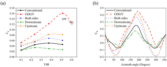
Figure 8.
(a) Power efficiency, and (b) variations as a function of the azimuth angle for a Savonius rotor with different double-deflector arrangements.
According to Figure 8a, the ODGV system represents the most effective configuration among the assessed evaluations for the WAG-RH. This system not only enhanced the across the operational range but also increased the maximum operational range from a TSR of 0.5 to 0.6, known as the Extended Performance Point (EPP). In other words, the peak occurs at a TSR of 0.5 with the ODGV system, whereas both the conventional rotor and the double-deflector arrangements reach their peak at a TSR of 0.4. Notably, at a TSR of 0.5, the ODGV system achieves a 300% increase in compared to the conventional rotor, as the local rises from 0.04 to 0.16. Other WAG-RH configurations have not been able to achieve an effective EPP. However, positioning double deflectors upstream and on both lateral sides of the rotor can enhance to 0.08 and 0.06, increasing performance by up to 100% and 50%, respectively, compared to the conventional rotor at TSR = 0.5. In contrast, placing deflectors downstream of the rotor proves ineffective, resulting in a reduction in across all TSRs. Figure 8b shows the variations in throughout a complete rotation at TSR = 0.5. It is evident that Savonius rotors—whether equipped with WAG-RH or not—exhibit positive values at the initial azimuth angle. This observation indicates that this drag-based rotor possesses self-starting capability without requiring initial torque. Furthermore, rotors integrated with the ODGV system and those with upstream and both-side deflector configurations demonstrate an improvement in values ranging from 52% to 80% compared to the conventional rotor at an azimuth angle of 180°. Conversely, positioning deflectors downstream of the rotor reduced the , making this configuration insufficient. To further elucidate the flow structure around the rotor, the pressure, velocity, and vorticity fields are presented in Figure 9, Figure 10, and Figure 11, respectively.
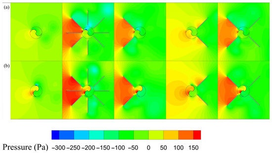
Figure 9.
Pressure field around the rotor for different double-deflector arrangements: (a) , and (b) .
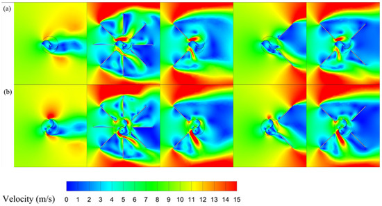
Figure 10.
Velocity field around the rotor for different double-deflector arrangements: (a) , and (b) .
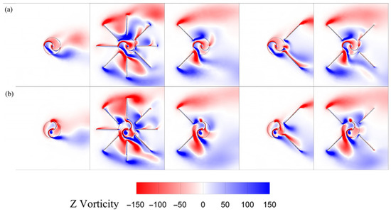
Figure 11.
Z-vorticity field around the rotor for different double-deflector arrangements: (a) , and (b) .
According to Figure 9, at both azimuthal angles of 90° and 180°, incorporating deflectors on the rotor’s suction side modifies the pressure distribution around the rotor. This change produces a high-pressure zone of approximately 150 Pa adjacent to the suction side at both rotor positions. Notably, the ODGV configuration, as well as upstream and dual-side deflector arrangements, generate high-pressure regions around 100 Pa on the concave side of the advancing bucket, thereby increasing the overall pressure differential and enhancing torque potential. In contrast, installing downstream deflectors prevents the formation of a concentrated high-pressure zone; instead, the high-pressure zone between 100 Pa to 150 Pa is distributed along the suction side, affecting both the concave side of the advancing bucket and the convex side of the returning bucket. This altered distribution negatively impacts the convex side of the returning bucket, resulting in reduced torque; therefore, the downstream deflector is not an effective design without significant flow structure improvements compared to the conventional control case rotor.
The control case demonstrates a typical wake pattern with pronounced flow separation and a low-velocity recirculation zone downstream of the rotor. Adding deflectors significantly alters the flow field, particularly in the ODGV and in upstream or both-side configurations. These arrangements produce a more directed, accelerated flow upstream, increasing the inflow velocity on the convex side of the advancing bucket to 15 m/s and shielding the returning bucket from adverse counterproductive flow effects at an azimuth angle of 180°. Such arrangements lead to a more concentrated high-velocity zone on the rotor’s suction side and a reduction in wake-induced energy losses in the rotor discharge region. Upstream deflectors alone offer partial shielding and inflow guidance, whereas downstream deflectors mainly influence wake symmetry without greatly improving incoming flow conditions. At an azimuth angle of 90°, placing deflectors on the rotor’s suction side markedly improves flow acceleration and guidance around the convex side of the returning bucket tip, raising the inflow velocity by 15 m/s. This change reduces the stagnation zone around the rotor and enhances torque.
According to Figure 11, at an azimuth angle of 180°, the positive Z-vorticity field—aligned with the rotor’s direction of rotation on the convex side of the advancing bucket—facilitates rotation when deflectors are positioned on the rotor’s suction side. This positive vorticity originates in the region where the inflow velocity increases to 15 m/s. Under the same configuration, a negative Z-vorticity field is observed at the deflector tips, coinciding with the accelerated inflow region and maintaining alignment with the rotor’s rotational direction. At an azimuth angle of 90°, favorable positive Z-vorticity is evident at the convex portion of the returning bucket, indicating improved inflow velocity. Also, when deflectors are positioned on the rotor’s suction side, a negative Z-vorticity field develops tangentially to the convex side of the returning bucket, further aiding rotation. In contrast, this beneficial vorticity pattern is absent in both the control case and the downstream-only deflector configuration. Overall, the analysis shows that strategic deflector placement—especially the combined upstream–downstream configuration—can effectively shape local flow structures, enhancing energy capture and reducing wake losses in Savonius VAWTs.
4.2. Triple-Deflector Arrangement
This section examines the triple-deflector configuration, designated as the WAG-RH, which involves strategically placing three deflector bundles on the upstream, downstream, and both lateral sides of the rotor within the RH domain. Its performance is compared with that of a traditional Savonius rotor and the ODGV system specifically designed for the WAG-RH. Figure 12 presents the performance map of the Savonius rotor, incorporating the triple-deflector configuration into the evaluation.
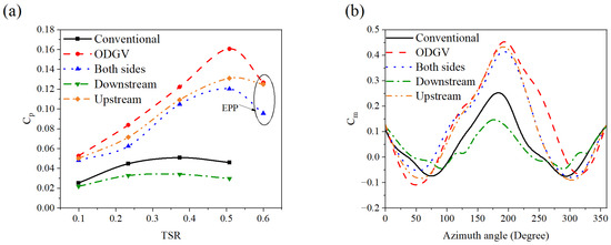
Figure 12.
(a) Power efficiency, and (b) variations as a function of the azimuth angle for a Savonius rotor with different triple-deflector arrangements.
According to Figure 12, positioning the triple-deflector configuration upstream of the rotor and on both sides of the RH increases local values from 0.04 to 0.13 and 0.14, representing increases of up to 225% and 200%, respectively, compared with the conventional rotor at a TSR of 0.5. These configurations also extend the operational range and provide EPP, raising the maximum TSR from 0.5 to 0.6, similar to the ODGV configuration. However, despite these improvements, the triple-deflector configuration remains slightly less effective than the ODGV. Placing a deflector downstream has a detrimental effect on the , mirroring the trend observed in the double-deflector arrangement. As shown in Figure 12b, downstream placement reduces at an azimuth angle of 180° compared with the conventional rotor. In contrast, the upstream and both-side deflector configurations yield nearly identical improvements of about 72%, although still marginally below ODGV performance. To further clarify the flow structure surrounding the rotor, the pressure and velocity fields are presented in Figure 13 and Figure 14, respectively.
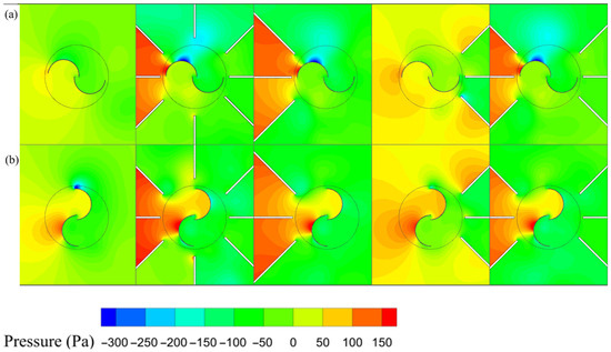
Figure 13.
Pressure field around the rotor with different triple-deflector arrangements: (a) , and (b) .
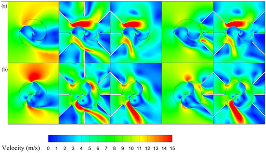
Figure 14.
Velocity field around the rotor with different triple-deflector arrangements: (a) , (b) .
According to Figure 13, adding deflectors on the rotor’s suction side significantly modifies the pressure distribution at both azimuthal angles of 90° and 180°. At 180°, the middle deflector in the triple configuration is specifically designed to enhance pressure accumulation on the convex side of the advancing bucket compared to the double-deflector configuration, resulting in a high-pressure zone of about 150 Pa adjacent to the rotor’s suction side and advancing bucket tip. This is accompanied by a negative pressure zone on the convex side—absent in conventional rotor and downstream-deflector configurations, where pressure is more uniformly distributed without notable accumulation. At 90°, configurations involving the ODGV, upstream, and both-side deflectors generate localized high-pressure regions around the rotor’s suction side. These high-pressure regions are directed toward the convex side of the returning bucket and the concave side of the advancing bucket, supported by the middle deflector. This creates a pressure differential between the suction and discharge sections—due to pressure accumulation around the advancing bucket’s concave side and the returning bucket’s convex side—thus enhancing efficiency. This localized pressure effect is not observed in conventional rotors or downstream-only configurations, where pressure remains broadly distributed rather than concentrated.
In this configuration, which closely resembles the flow structure of the double-deflector arrangement, deflector bundles placed on the rotor’s suction side effectively direct and accelerate the inflow upstream. This increases the inflow velocity on the convex side of the advancing bucket to 15 m/s while shielding the returning bucket from adverse flow effects at an azimuth angle of 180°. These configurations produce a concentrated high-velocity zone on the rotor’s suction side, reducing wake-induced energy loss in the discharge region. At 90°, the flow structure remains consistent with the double-deflector configuration, as the deflectors continue to promote accelerated flow on the convex side of the returning bucket when situated on the suction side. Since the velocity structure closely matches that of the double-deflector arrangement, a Z-vorticity field for the triple configuration is not presented here.
4.3. Oblique Deflector Arrangement
This section analyzes the oblique deflector configuration, designated as the WAG-RH, which strategically places two deflectors oriented in the crosswind and upwind directions within the RH domain. Figure 15 compares the oblique deflector arrangements with both the conventional rotor and ODGV configurations.
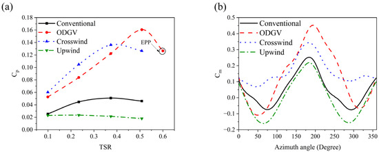
Figure 15.
(a) Power efficiency, and (b) variations as a function of azimuth angle for a Savonius rotor with different oblique deflector arrangements.
According to Figure 15, the oblique deflector configurations do not provide EPP or extend the operational range. However, the crosswind deflector increases the local from 0.04 to 0.13, representing increases by up to 225% compared to the conventional design at a TSR of 0.5, and enhances the across the TSR range of 0.1 to 0.4. It also achieves up to a 20% improvement in the relative to the ODGV configuration, as the local is increased from 0.08 to 0.1 at TSR = 0.25. In contrast, the upwind configuration (WAG-RH) reduces the compared to the conventional rotor, indicating it is not optimal. Figure 15b illustrates that the crosswind configuration improves the by up to 40% over the conventional case at an azimuth angle of 180°. Moreover, it outperforms the ODGV configuration in the across azimuth angles from 0° to 90° and 270° to 360°, provided the concave side of the advancing bucket faces the wind. To further clarify the flow structure around the rotor, pressure, velocity, and vorticity fields are shown in Figure 16, Figure 17, and Figure 18, respectively.
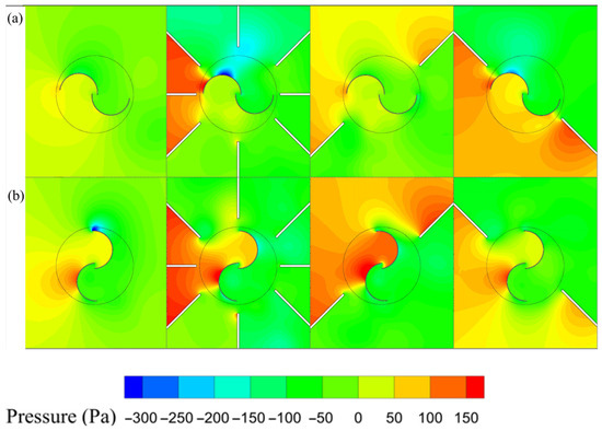
Figure 16.
Pressure field around the rotor for different oblique deflector arrangements: (a) , and (b) .
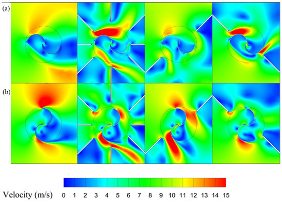
Figure 17.
Velocity field around the rotor for different oblique deflector arrangements: (a) , and (b) .
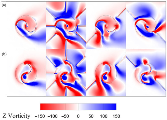
Figure 18.
Z-vorticity field around the rotor for different oblique deflector arrangements: (a) , and (b) .
According to Figure 16a, the implementation of crosswind oblique deflectors significantly alters the pressure field, leading to increased aerodynamic loading. The crosswind arrangement, similar to the ODGV configuration, achieves the most efficient pressure accumulation at an azimuth angle of 180°. In contrast, the upwind configuration, despite generating a localized pressure buildup in front of the rotor near the convex section of the advancing bucket, exhibits the poorest aerodynamic performance compared to ODGV and other configurations, including the crosswind, as well as the previous double and triple configurations (see Figure 9 and Figure 13). The lower deflector in the other configurations helps distribute high-pressure zones on the convex side of the returning bucket. However, in the upwind configuration, the absence of a lower deflector adversely affects pressure distribution on the returning bucket, preventing effective high-pressure localization and thereby reducing the torque. Regarding Figure 16b, the crosswind configuration concentrates a high-pressure zone of 150 Pa primarily on the concave side of the advancing bucket and the convex portion of the returning bucket, with greater intensity than the ODGV configuration. This focused pressure distribution enhances torque performance. In contrast, the upwind configuration fails to localize pressure effectively at optimal locations and does not create a sufficient pressure differential between the advancing and returning buckets. The high-pressure zone is mainly concentrated on the convex side of the returning bucket, resembling the pressure pattern of a conventional rotor. As a result, this configuration does not contribute to a torque improvement due to misalignment between the pressure field and blade motion.
According to Figure 17a, at an azimuth of 180°, the oblique upwind configuration effectively directs inflow towards the convex side of the advancing bucket, achieving performance comparable to the ODGV configuration. However, the absence of a lower deflector—similar to the downstream configurations in both double and triple configurations (see Figure 10 and Figure 14)—leads to an extended stagnation zone on the convex side of the returning bucket. This negatively impacts aerodynamic performance, indicating that the upwind configuration fails to shield the returning bucket from adverse flow and that its flow structure closely resembles that of the conventual rotor without a significant improvement. In contrast, although the crosswind configuration produces significantly less flow acceleration toward the rotor than the ODGV configuration, it avoids a large stagnation zone around the buckets. Furthermore, the deflector arrangements effectively guide the flow. As shown in Figure 17b, the crosswind configuration accelerates inflow on the convex portions of both the advancing and returning buckets, resulting in increased torque at an azimuth angle of 90° compared to the ODGV system. Conversely, the upwind configuration shows no meaningful flow acceleration; the flow field on the convex side of the returning bucket closely matches the conventional case, and the high-velocity region at the advancing bucket tip is absent. This results in performance inferior to the conventional rotor.
According to Figure 18, the crosswind configuration produces negative Z-vorticity at the tip of the deflector on the suction side, coinciding with an accelerated inflow. In contrast, the upwind configuration exhibits positive, favorable Z-vorticity on the convex side of the advancing bucket, similar to the ODGV configuration. However, due to the lack of directional flow guidance by the deflector on the rotor’s suction side, negative Z-vorticity does not form in this section—mirroring the conventional and downstream-deflector cases (see Figure 11)—which reduces rotor efficiency. Figure 18b shows that, in the crosswind configuration, negative Z-vorticity is tangential to the convex side of the returning bucket, consistent with the ODGV configuration. Conversely, the upwind configuration, which retains the conventional flow structure, lacks this negative Z-vorticity; instead, positive Z-vorticity develops near the discharge zone at the lower deflector’s tip, which is considered unfavorable given the rotor’s orientation.
4.4. Straight Deflector Arrangement
This section examines the straight deflector configuration, designated as the WAG-RH, which strategically places four deflectors on both the suction and discharge sides, as well as above and below the rotor—forming a dual-plane arrangement. In this setup, two deflectors are positioned axially (one above and one below), while the remaining two are arranged radially within the suction and discharge zones. All components are located within the RH domain. Figure 19 presents a comparative analysis of the straight-deflector arrangements against both the conventional rotor and the ODGV configurations.
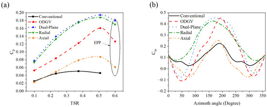
Figure 19.
(a) Power efficiency, and (b) variations as a function of azimuth angle for a Savonius rotor with different straight deflector arrangements.
According to Figure 19a, implementing a straight deflector configuration—regardless of the arrangement—for the WAG-RH application enhances EPP by increasing the maximum TSR from 0.5 to 0.6. Notably, the radial and dual-plane configurations, which deliver nearly identical performance, improve the by approximately 385% compared to the conventional rotor by increasing the local value from 0.04 to 0.194, at a TSR of 0.5 and by up to 25% compared to the ODGV configuration with a of 0.16 at this TSR. Finally, the axial configuration, which represents the weakest among the straight-deflector configurations, still achieves a 100% improvement in the local over the conventional rotor at the same TSR. Figure 19b shows that variations between 90° to 270° are largely comparable for the radial and dual-plane configurations.
Across most azimuth angles, these configurations exhibit higher values compared to the ODGV configuration, underscoring their enhanced torque capabilities. Additionally, the axial configuration demonstrates a superior than the conventional case at an azimuth angle of 180°. To further clarify the flow structure around the rotor with straight deflectors, the pressure, velocity, and vorticity fields are presented in Figure 20, Figure 21, and Figure 22, respectively.
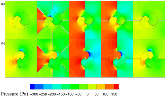
Figure 20.
Pressure field around the rotor for different straight deflector arrangements: (a) , and (b) .
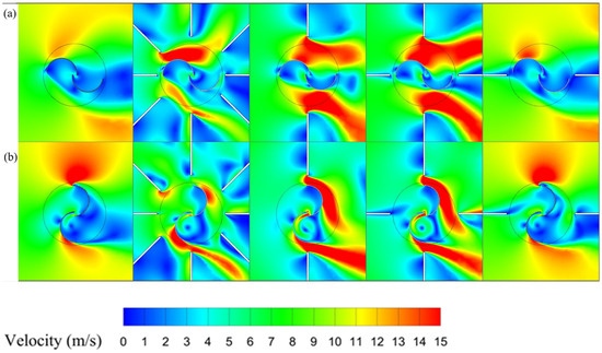
Figure 21.
Velocity field around the rotor for different straight deflector arrangements: (a) , and (b) .
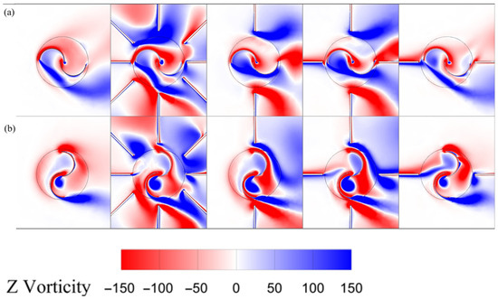
Figure 22.
Z-vorticity field around the rotor for different straight deflector arrangements: (a) , and (b) .
According to Figure 20a, both the dual-plane and axial deflector configurations trap a similar high-pressure zone of 150 Pa on the rotor’s suction side, resulting in nearly identical values (see Figure 19). The pressure accumulation on the rotor suction side in these configurations is more pronounced than in the ODGV system, resulting in superior performance. In contrast, the radial deflector arrangement demonstrates no significant pressure accumulation—similar to the conventional rotor—yielding variations more in line with conventional performance. Figure 20b shows that the benefits of the axial and dual-plane configurations arise from high-pressure accumulation across the entire suction side, rather than localized on the returning bucket’s convex side. This distribution covers both the concave side of the advancing bucket and the convex side of the returning bucket, resulting in a significant pressure differential around the rotor, which in turn enhances the torque. Although the radial deflector does not exhibit substantial suction-side pressure accumulation, its ability to effectively guide the flow still contributes to performance improvements over the conventional rotor.
According to Figure 21a, the dual-plane and axial deflectors effectively direct the inflow toward the rotor, achieving a velocity of 15 m/s on the convex side of the advancing bucket—an effect that is more pronounced than in the ODGV configuration. When positioned radially, the deflectors create a high-velocity zone on the convex portion of the advancing bucket, more pronounced than in the conventional case. As shown in Figure 21b, the axial and dual-plane configurations accelerate flow on the convex sides of both the returning and advancing buckets, thereby facilitating rotor rotation. The flow acceleration achieved by these two configurations exceeds that of the ODGV configuration. The radial configuration, while closely resembling the flow structure of the conventional case, benefits from a reduced stagnation zone due to the presence of the downstream deflector.
According to Figure 22a, both the axial and dual-plane deflector configurations facilitate the generation of positive vorticity on the upper surface of the rotor and negative vorticity on the lower surface, consistent with the direction of rotor rotation. In contrast, the vorticity field for the radial configuration shows little deviation from that of the conventional case. Figure 22b shows that the favorable vorticity formation on the convex side of the advancing and returning bucket tips in the dual-plane and axial configurations is more pronounced than in the ODGV system, resulting in enhanced performance. For the radial configuration, the vorticity field is nearly identical to the conventional case; however, the generation of positive Z-vorticity on the concave side of the advancing bucket contributes to performance gains.
5. Performance Summary
In this section, we will provide a comprehensive summary of the performance of various rotors, which includes the AVE across all TSR ranges. We will compare different rotors with the WAG-RH rotor and a conventional rotor to evaluate their overall performance. Additionally, the values at TSR = 0.5 will be assessed against the conventional rotor to highlight any improvements. The performance summary is presented in Table 5.
Table 5.
Performance summary.
According to Table 5, the WAG-RH configurations featuring double and oblique deflectors are unable to extend the TSR ranges and provide an EPP. In contrast, configurations utilizing straight deflectors and a triple-deflector arrangement with upstream and both-side orientations successfully achieve an EPP. With respect to the AVE , the WAG-RH with downstream deflectors and upwind arrangements does not demonstrate an increase in the AVE when compared to the conventional rotor; thus, these configurations are not recommended for WAG-RH applications. A similar pattern is observed for the local at TSR = 0.5, where the values associated with these configurations are lower than those of the conventional case. However, the dual-plane and radial deflector configurations for straight arrangements, for the WAG-RH design, demonstrate a substantial increase of 385% in the local compared to the conventional rotor. Following closely, the ODGV configuration exhibits a 300% improvement, underscoring their operational efficiency. Notably, the dual-plane configuration achieves the highest enhancements in both the AVE and local , positioning it as the most effective design among the evaluated configurations.
6. Conclusions and Future Directions
This study examined the impact of various deflector configurations, specifically the WAG-RH, on the aerodynamic performance of the Savonius VAWT. The analysis covered several deflector arrangements, including double, triple, oblique, and straight configurations, comparing their effectiveness with both the ODGV WAG-RH and conventional rotor designs. For the ODGV configuration, the operational range extends from 0.5 to 0.6, corresponding to the EPP, also achieving up to a 300% increase in the compared to the conventional rotor at TSR = 0.5. In contrast, the double-deflector configuration, when installed upstream of the rotor, improves the by up to 100% but fails to achieve EPP. The triple deflector configuration performs best when positioned upstream of the RH, enhancing the by 255% at TSR = 0.5 and successfully achieving EPP. In contrast, oblique arrangements do not achieve EPP; however, the crosswind WAG-RG increased the by up to 25% compared to the ODGV system. Conversely, the upwind configuration proves inefficient, similar to the downstream double and triple configurations. Overall, the straight configuration emerges as the most effective configuration. All straight arrangements achieved EPP, with the dual-plane and radial configurations delivering nearly identical performance—improving the by 385% over the conventional rotor and by up to 25% compared to the ODGV WAG-RH rotor at TSR = 0.5. The dual-plane configuration of the rotor for the WAG-RH has not only enhanced the local but has also resulted in a 264.3% increase in the AVE compared to the conventional rotor. Consequently, this configuration may be regarded as the optimal design for the WAG-RH.
The introduction of the WAG-RH invariably incorporates an external device into the system; however, its design is structurally straightforward and employs conventional sheet-metal or lightweight composite fabrication techniques. Unlike active flow-control systems, these deflectors do not possess any moving parts, do not require auxiliary power input, and can be conveniently integrated into rooftop installations and urban applications without necessitating significant structural reinforcement. Consequently, the incremental costs associated with the manufacturing and installation of the WAG-RH are anticipated to be minimal in comparison to the aerodynamic efficiency gains that they provide. Therefore, while an extensive techno-economic assessment is outside the scope of this study, it is reasonable to conclude that the simplicity and low production costs of the WAG-RH will make this approach economically viable for small-scale wind energy applications in urban environments. Future research endeavors should encompass a comprehensive techno-economic assessment of WAG-RH systems to augment the aerodynamic analysis. Such investigations may focus on evaluating manufacturing costs, durability, and the integration of these systems into rooftop structures. Additionally, an analysis of the payback period and the levelized cost of energy (LCOE) will be crucial. It is also advisable to conduct sensitivity analyses concerning wind speed, material selection for both rotor buckets and deflectors, and electricity pricing in order to ascertain the practical feasibility of the concept. Furthermore, given that the rotors are installed on the rooftop, it is advisable to investigate the impact of wind gusts on rotor performance while incorporating the Discrete Phase Model (DPM) into the simulation. Additionally, it is advisable to develop a 3D model to assess the influence of turbine slope angles and the potential blockage effects from neighboring buildings. This analysis should employ a more sophisticated turbulence model, such as Large Eddy Simulation (LES), for enhanced precision.
Author Contributions
Conceptualization, F.G. and M.M.; methodology, F.G. and M.M.; software, F.G.; validation, F.G. and S.R.M.; formal analysis, F.G.; investigation, F.G. and S.R.M.; resources, F.G., S.F. and M.M.; data curation, F.G., M.M., S.R.M. and M.S.; writing—original draft preparation, S.F., F.G. and M.S.; writing—review and editing, S.F., M.M., M.S. and S.R.M.; visualization, F.G.; supervision, M.M. and M.S.; project administration, M.M. and M.S.; funding acquisition, F.G. and M.S. All authors have read and agreed to the published version of the manuscript.
Funding
This research received no external funding.
Data Availability Statement
The original contributions presented in this study are included in the article. Further inquiries can be directed to the corresponding author.
Conflicts of Interest
The authors declare no conflict of interest.
Correction Statement
This article has been republished with a minor correction to the Data Availability Statement. This change does not affect the scientific content of the article.
Nomenclature
The following nomenclature are used in this manuscript:
| Symbols | |
| Inlet flow velocity (m/s) | |
| A | Swept area (m2) |
| Torque (N·m) | |
| Output power (W) | |
| Rotor radius (m) | |
| Torque coefficient | |
| Power coefficient | |
| Greek | |
| Azimuth angle (Degree) | |
| Viscosity () | |
| Angular velocity (rad/s) | |
| Density (kg/m3) | |
| Rotor solidity | |
| Subscript | |
| t | Turbulence |
| Abbreviations | |
| VAWT | Vertical-axis wind turbine |
| HAWT | Horizontal-axis wind turbine |
| CFD | Computational fluid dynamic |
| CFL | Courant–Friedrichs–Lewy (Courant Number) |
| URANS | Unsteady Reynolds Averaged Naiver Stokes |
| TSR | Tip speed ratio |
| ODGV | Omni-directional guide vanes |
| WAG-RH | Wind accelerator and guiding rotor houses |
| RH | Rotor houses |
| EPP | Extended performance point |
| MAPE | Mean Absolute Percentage Error |
| APE | Absolute Percentage Error |
| RSME | Root Mean Square Error |
| Signs | |
| ↓ | Decrease |
| ↑ | Increase |
| ☑ | Present |
| ☒ | Absent |
References
- Petrychenko, O.; Levinskyi, M.; Goolak, S.; Lukoševičius, V. Prospects of solar energy in the context of greening maritime transport. Sustainability 2025, 17, 2141. [Google Scholar] [CrossRef]
- Lu, K.-H.; Hong, C.-M.; Lian, J.; Cheng, F.-S. A Review of Synergies Between Advanced Grid Integration Strategies and Carbon Market for Wind Energy Development. Energies 2025, 18, 590. [Google Scholar] [CrossRef]
- Mignogna, D.; Szabó, M.; Ceci, P.; Avino, P. Biomass energy and biofuels: Perspective, potentials, and challenges in the energy transition. Sustainability 2024, 16, 7036. [Google Scholar] [CrossRef]
- Elkodama, A.; Ismaiel, A.; Abdellatif, A.; Shaaban, S.; Yoshida, S.; Rushdi, M.A. Control methods for horizontal axis wind turbines (HAWT): State-of-the-art review. Energies 2023, 16, 6394. [Google Scholar] [CrossRef]
- Seifi Davari, H.; Seify Davari, M.; Botez, R.M.; Chowdhury, H. Advancements in vertical axis wind turbine technologies: A comprehensive review. Arab. J. Sci. Eng. 2025, 50, 2169–2216. [Google Scholar] [CrossRef]
- Bošnjaković, M.; Veljić, N.; Hradovi, I. Perspectives of Building-Integrated Wind Turbines (BIWTs). Smart Cities 2025, 8, 55. [Google Scholar] [CrossRef]
- Tjiu, W.; Marnoto, T.; Mat, S.; Ruslan, M.H.; Sopian, K. Darrieus vertical axis wind turbine for power generation I: Assessment of Darrieus VAWT configurations. Renew. Energy 2015, 75, 50–67. [Google Scholar] [CrossRef]
- Moghimi, M.; Motawej, H. Investigation of effective parameters on Gorlov vertical axis wind turbine. Fluid Dyn. 2020, 55, 345–363. [Google Scholar] [CrossRef]
- Omer-Alsultan, G.; Alsahlani, A.A.; Mohamed-Alsultan, G.; Abdulkareem-Alsultan, G.; Nassar, M.F.; Kurniawan, T.A.; Taufiq-Yap, Y.H. Towards zero emission: Exploring innovations in wind turbine design for sustainable energy a comprehensive review. Serv. Oriented Comput. Appl. 2024, 1–37. [Google Scholar] [CrossRef]
- Jebelli, A.; Lotfi, N.; Zare, M.S.; Yagoub, M.C. A comprehensive review of effective parameters to improve the performance of the Savonius turbine using a computational model and comparison with practical results. Water-Energy Nexus 2024, 7, 266–274. [Google Scholar] [CrossRef]
- Vadhyar, A.; Sridhar, S.; Reshma, T.; Radhakrishnan, J. A critical assessment of the factors associated with the implementation of rooftop VAWTs: A review. Energy Convers. Manag. X 2024, 22, 100563. [Google Scholar] [CrossRef]
- Sumiati, R.; Dinata, U.G.S.; Saputra, D.A. Enhancing savonius rotor performance with wavy pattren in the concave surface-A short review. In Proceedings of the International Conference on Mechanical Engineering and Emerging Technologies (ICOMEET2023), Padang, Indonesia, 1 November 2023; AIP Publishing: Melville, NY, USA, 2025. [Google Scholar]
- Tahani, M.; Rabbani, A.; Kasaeian, A.; Mehrpooya, M.; Mirhosseini, M. Design and numerical investigation of Savonius wind turbine with discharge flow directing capability. Energy 2017, 130, 327–338. [Google Scholar] [CrossRef]
- Lajnef, M.; Mosbahi, M.; Abid, H.; Driss, Z.; Amato, E.; Picone, C.; Sinagra, M.; Tucciarelli, T. Numerical and experimental investigation for helical savonius rotor performance improvement using novel blade shapes. Ocean Eng. 2024, 309, 118357. [Google Scholar] [CrossRef]
- Nasef, M.H.; Asaad Awad, B.N.; EL-Askary, W.A. Installing new additional blades arrangement for improving Savonius rotor performance. Wind Eng. 2025, 49, 536–556. [Google Scholar] [CrossRef]
- Marinić-Kragić, I.; Vučina, D.; Milas, Z. Computational analysis of Savonius wind turbine modifications including novel scooplet-based design attained via smart numerical optimization. J. Clean. Prod. 2020, 262, 121310. [Google Scholar] [CrossRef]
- Al-Ghriybah, M.; Didane, D.H. Performance improvement of a Savonius wind turbine using wavy concave blades. CFD Lett. 2023, 15, 32–44. [Google Scholar] [CrossRef]
- Al-Gburi, K.A.H.; Alnaimi, F.B.I.; Al-quraishi, B.A.J.; Tan, E.S.; Kareem, A.K. Enhancing Savonius Vertical Axis Wind Turbine Performance: A Comprehensive Approach with Numerical Analysis and Experimental Investigations. Energies 2023, 16, 4204. [Google Scholar] [CrossRef]
- Harsito, C.; Tjahjana, D.D.D.P.; Kristiawan, B. Savonius turbine performance with slotted blades. In Proceedings of the 5th International Conference on Industrial, Mechanical, Electrical, and Chemical Engineering 2019 (ICIMECE 2019), Surakarta, Indonesia, 17–18 September 2019; AIP Publishing: Melville, NY, USA, 2020. [Google Scholar]
- Ghafoorian, F.; Mirmotahari, S.R.; Mehrpooya, M.; Akhlaghi, M. Aerodynamic performance and efficiency enhancement of a Savonius vertical axis wind turbine with Semi-Directional Curved Guide Vane, using CFD and optimization method. J. Braz. Soc. Mech. Sci. Eng. 2024, 46, 443. [Google Scholar] [CrossRef]
- Shahizare, B.; Nazri Bin Nik Ghazali, N.; Chong, W.T.; Tabatabaeikia, S.S.; Izadyar, N. Investigation of the Optimal Omni-Direction-Guide-Vane Design for Vertical Axis Wind Turbines Based on Unsteady Flow CFD Simulation. Energies 2016, 9, 146. [Google Scholar] [CrossRef]
- Mohammadi, M.; Mohammadi, R.; Ramadan, A.; Mohamed, M. Numerical investigation of performance refinement of a drag wind rotor using flow augmentation and momentum exchange optimization. Energy 2018, 158, 592–606. [Google Scholar] [CrossRef]
- Rajpar, A.H.; Ali, I.; Eladwi, A.E.; Bashir, M.B. Recent Development in the Design of Wind Deflectors for Vertical Axis Wind Turbine: A Review. Energies 2021, 14, 5140. [Google Scholar] [CrossRef]
- Chitura, A.G.; Mukumba, P.; Lethole, N. Enhancing the Performance of Savonius Wind Turbines: A Review of Advances Using Multiple Parameters. Energies 2024, 17, 3708. [Google Scholar] [CrossRef]
- Noman, A.A.; Tasneem, Z.; Sahed, M.F.; Muyeen, S.M.; Das, S.K.; Alam, F. Towards next generation Savonius wind turbine: Artificial intelligence in blade design trends and framework. Renew. Sustain. Energy Rev. 2022, 168, 112531. [Google Scholar] [CrossRef]
- Layeghmand, K.; Ghiasi Tabari, N.; Zarkesh, M. Improving efficiency of Savonius wind turbine by means of an airfoil-shaped deflector. J. Braz. Soc. Mech. Sci. Eng. 2020, 42, 528. [Google Scholar] [CrossRef]
- Mohamed, M.; Janiga, G.; Pap, E.; Thévenin, D. Optimization of Savonius turbines using an obstacle shielding the returning blade. Renew. Energy 2010, 35, 2618–2626. [Google Scholar] [CrossRef]
- Salleh, M.B.; Kamaruddin, N.M. Power performance and flow structure analysis of a deflector-augmented savonius hydrokinetic turbine under variable flow speeds. Ocean Eng. 2025, 325, 120789. [Google Scholar] [CrossRef]
- Chong, W.T.; Fazlizan, A.; Poh, S.C.; Pan, K.C.; Hew, W.P.; Hsiao, F.B. The design, simulation and testing of an urban vertical axis wind turbine with the omni-direction-guide-vane. Appl. Energy 2013, 112, 601–609. [Google Scholar] [CrossRef]
- Kalluvila, J.B.S.; Sreejith, B. Numerical and experimental study on a modified Savonius rotor with guide blades. Int. J. Green Energy 2018, 15, 744–757. [Google Scholar] [CrossRef]
- Manganhar, A.L.; Rajpar, A.H.; Luhur, M.R.; Samo, S.R.; Manganhar, M. Performance analysis of a savonius vertical axis wind turbine integrated with wind accelerating and guiding rotor house. Renew. Energy 2019, 136, 512–520. [Google Scholar] [CrossRef]
- Wenehenubun, F.; Saputra, A.; Sutanto, H. An Experimental Study on the Performance of Savonius Wind Turbines Related with the Number of Blades. Energy Procedia 2015, 68, 297–304. [Google Scholar] [CrossRef]
- Sheidani, A.; Salavatidezfouli, S.; Stabile, G.; Rozza, G. Assessment of URANS and LES methods in predicting wake shed behind a vertical axis wind turbine. J. Wind Eng. Ind. Aerodyn. 2023, 232, 105285. [Google Scholar] [CrossRef]
- Menter, F.R. Review of the shear-stress transport turbulence model experience from an industrial perspective. Int. J. Comput. Fluid Dyn. 2009, 23, 305–316. [Google Scholar] [CrossRef]
- Meana-Fernández, A.; Fernández Oro, J.M.; Argüelles Díaz, K.M.; Velarde-Suárez, S. Turbulence-Model Comparison for Aerodynamic-Performance Prediction of a Typical Vertical-Axis Wind-Turbine Airfoil. Energies 2019, 12, 488. [Google Scholar] [CrossRef]
- Spalart, P.; Allmaras, S. A one-equation turbulence model for aerodynamic flows. In Proceedings of the 30th Aerospace Sciences Meeting and Exhibit, Reno, NV, USA, 6–9 January 1992; p. 439. [Google Scholar]
- Didane, D.H.; Rosly, N.; Zulkafli, M.F.; Shamsudin, S.S. Numerical investigation of a novel contra-rotating vertical axis wind turbine. Sustain. Energy Technol. Assess. 2019, 31, 43–53. [Google Scholar] [CrossRef]
- Moghimi, M.; Motawej, H. Developed DMST model for performance analysis and parametric evaluation of Gorlov vertical axis wind turbines. Sustain. Energy Technol. Assess. 2020, 37, 100616. [Google Scholar] [CrossRef]
- Bianchini, A.; Balduzzi, F.; Bachant, P.; Ferrara, G.; Ferrari, L. Effectiveness of two-dimensional CFD simulations for Darrieus VAWTs: A combined numerical and experimental assessment. Energy Convers. Manag. 2017, 136, 318–328. [Google Scholar] [CrossRef]
- Bumrungthaichaichan, E. How can the appropriate near-wall grid size for gas cyclone CFD simulation be estimated? Powder Technol. 2022, 396, 327–344. [Google Scholar] [CrossRef]
- Marsh, P.; Ranmuthugala, D.; Penesis, I.; Thomas, G. The influence of turbulence model and two and three-dimensional domain selection on the simulated performance characteristics of vertical axis tidal turbines. Renew. Energy 2017, 105, 106–116. [Google Scholar] [CrossRef]
- Harris, M. Flow Feature Aligned Mesh Generation and Adaptation. Ph.D. Thesis, University of Sheffield, Sheffield, UK, 2013. [Google Scholar]
- Balduzzi, F.; Bianchini, A.; Ferrara, G.; Ferrari, L. Dimensionless numbers for the assessment of mesh and timestep requirements in CFD simulations of Darrieus wind turbines. Energy 2016, 97, 246–261. [Google Scholar] [CrossRef]
- Trivellato, F.; Castelli, M.R. On the Courant–Friedrichs–Lewy criterion of rotating grids in 2D vertical-axis wind turbine analysis. Renew. Energy 2014, 62, 53–62. [Google Scholar] [CrossRef]
- Chegini, S.; Asadbeigi, M.; Ghafoorian, F.; Mehrpooya, M. An investigation into the self-starting of darrieus-savonius hybrid wind turbine and performance enhancement through innovative deflectors: A CFD approach. Ocean Eng. 2023, 287, 115910. [Google Scholar] [CrossRef]
- Ghafoorian, F.; Hosseini Rad, S.; Moghimi, M. Enhancing Self-Starting Capability and Efficiency of Hybrid Darrieus–Savonius Vertical Axis Wind Turbines with a Dual-Shaft Configuration. Machines 2025, 13, 87. [Google Scholar] [CrossRef]


Disclaimer/Publisher’s Note: The statements, opinions and data contained in all publications are solely those of the individual author(s) and contributor(s) and not of MDPI and/or the editor(s). MDPI and/or the editor(s) disclaim responsibility for any injury to people or property resulting from any ideas, methods, instructions or products referred to in the content. |
© 2025 by the authors. Licensee MDPI, Basel, Switzerland. This article is an open access article distributed under the terms and conditions of the Creative Commons Attribution (CC BY) license (https://creativecommons.org/licenses/by/4.0/).