Article

Global Stiffness Modeling of Robot Drilling System Incorporating End-Effector and Arm Flexibility Based on Virtual Joint Method

College of Mechanical and Electrical Engineering, China Jiliang University, Hangzhou 310018, China
*
Author to whom correspondence should be addressed.
Machines 2025, 13(9), 837; https://doi.org/10.3390/machines13090837
Submission received: 8 August 2025 / Revised: 1 September 2025 / Accepted: 6 September 2025 / Published: 9 September 2025

Abstract

In the new digital era, industrial robots are central to machining and flexible production in intelligent manufacturing. However, the rigidity of the six degrees-of-freedom (DOFs) serial robot is insufficient, which leads to chatter during machining and limits its application in high-precision machining, especially in the field of drilling, reaming and milling. A new method was proposed for modeling the global stiffness of the robot drilling system that incorporated the end-effector. Based on the virtual joint method and linear superposition principle, and considering the flexibility of the robot arm, the global stiffness model of the robot drilling system was established by simplifying the modeling process with dual quaternion. The results of the model validation experiments of deformation show that the maximum relative error of resultant end deformation is 8.80%, and the average relative error of resultant end deformation is 7.21%. This method provides a new method of global stiffness modeling for the robot drilling system, including the end-effector, and a new approach for stiffness improvement to overcoming the problem of insufficient robot stiffness in intelligent manufacturing industry.

1. Introduction

In intelligent manufacturing and Industry 4.0, industrial robots will become the core labor force. As intelligent industrial automation continues to advance, the use of industrial robots in production is on the rise [1,2]. Compared to the CNC machine tool, the core advantages of industrial robots lie in their exceptional flexibility, extensive work envelope, high cost-effectiveness, and the ability to quickly adapt to various tasks by changing end-effectors, making them ideal for flexible manufacturing. The six-DOFs serial robot can approach the machining position in a variety of postures by redundant degrees of freedom [3], which shows strong spatial flexibility and cost advantage in the manufacturing industry [4,5]. However, the structural characteristics of the serial robot lead to insufficient static stiffness, and the resulting machining error is the main factor restricting the serial robot in the actual machining task [6,7]. During the machining, due to the influence of various factors such as the dynamic stiffness and the natural frequency of the robot, the tool and the workpiece generate chatter, which greatly affects the dimensional accuracy and surface roughness of the machined hole [8,9]. Therefore, the numerical simulation analysis of stiffness is an important step for improving the stiffness of serial robots.

1.1. Related Works

At present, the modeling methods for robot stiffness are mainly divided into three categories, including finite element analysis (FEA) [7,10,11,12,13,14], matrix structure analysis (MSA) [15,16,17] and virtual joint method (VJM) [6,18,19,20,21,22]. Doukas et al. [10] took advantage of FEA to model the stiffness of the serial robot based on a CAD digital model and expressed the machining precision accurately and intuitively in the workspace with color coding. In order to better describe the accuracy of the robot stiffness model, Marie et al. [11] proposed a method to establish the elastic geometric model of the robot structure by combining FEA and a fuzzy inference system. Kermanian et al. [12] improved the speed of the FEA method by modeling the flexible rod with the rotation factor in the same direction. Raoofian et al. [15] calculated the Cartesian stiffness matrix of the manipulator through MSA and obtained the stiffness index of the Delta parallel robot to identify the influence of the manipulator on the external deflection. Cammarata [16] proposed an extended MSA method to achieve stiffness analysis of robots with parallelogram joints or inner loops without simplification. The VJM was first proposed by Salisbury and Gossellin [18]. The connecting rod was set to be rigid, the joint was set to be flexible and the virtual springs were applied to build the model. Subsequently, Klimchik et al. [19] improved the VJM by using analytical inversion of submatrices and a dedicated recursive method. On this basis, Dumas et al. [20] and Gao et al. [6] employed conservative congruence transformation (CCT) to analyze the translation and rotation of the end of the robot machining system and proposed a more efficient identification method of joint stiffness for six-DOFs serial robots.
Among the three modeling methods, the advantage of FEA method is that the physical model of the robot is decomposed into a large number of finite degrees of freedom units, which can obtain more accurate modeling results [13,14]. However, it requires a large number of calculations with the cooperation of the computer, and the modeling speed is slow. Unlike the FEA method, the MSA method simplifies the connecting rods into beams and nodes, which effectively reduces the calculation cost and achieves a reasonable balance between calculation time and accuracy [23], but inevitably reduces the modeling accuracy. The VJM, which describes elastic components as lumped parameter models [20], provides a simple method for modeling joint stiffness [22]. Compared with the other two methods, the centralized description of joint stiffness by the VJM greatly simplifies the process of identifying the stiffness of the robot. Moreover, the VJM has better performance in accuracy and computational efficiency and the best comprehensive usability [21]. However, the VJM also has limitations, as it assumes that the connecting components are completely rigid, while only the joints are elastic.
Based on the existing three modeling methods, the combined analysis or processing methods have been applied in recent years for in-depth analysis of stiffness models. Typical studies include the multi-body simulation method (MBS) for predicting the robot dynamic behavior [7,24,25], stiffness ellipsoid evaluation method for stiffness limitations identification [17], dexterity analysis by an inverse kinematic (IK) technique for optimal posture identification [22] and dual quaternion analysis method for simplifying the modeling process of robot stiffness [26,27].
Meanwhile, many scholars have conducted research in recent years on stiffness optimization to improve processing stability [6,7,22], dynamic behavior analysis for chatter suppression [7,28] and considering links weight to improve model accuracy [29]. These could be motivations for future research in the field of machining using robots.
However, most of the developed modeling methods for stiffness-of-robot drilling system were mainly carried out from the perspective of robot kinematics, and the overall stiffness model was not considered from the perspective of the robot and end-effector system and the arm flexibility. For this purpose, this work aims to develop a global stiffness model of the robot drilling system incorporating the end-effector and provide an approach of high computational efficiency for stiffness improvement analysis in robot machining stability solutions, based on the virtual joint method, combined with the dual quaternion analysis method for simplifying the modeling process and avoiding the occurrence of singular solutions, and considering the flexibility of the robot arm. A series of experiments was also conducted to verify the effectiveness of the proposed model.

1.2. Structure of the Paper

This paper is organized into four sections. Section 2 introduces the global stiffness modeling method of the robot drilling system, including the workstation components of the robot drilling system, the joint stiffness modeling method of drilling robot by the VJM and dual quaternion analysis method, the end-effector stiffness modeling method, and the overall stiffness modeling of the robot drilling system. Section 3 presents the stiffness model verification experiments and conducts the analysis of relative errors of end deformation for stiffness model validation. Finally, Section 4 summarizes the major contributions and results of this research.

2. The Global Stiffness Modeling of the Robot Drilling System

2.1. Robot Drilling Workstation

The workstation of the robot drilling system includes a drilling robot and peripheral equipment such as the drilling end-effector, auxiliary workbench, control cabinet and teach pendant, as shown in Figure 1.
The high-speed cutting electric spindle is applied as the end-effector of the robot drilling system, which is controlled by the frequency converter. The I/O signals of the drilling robot are used to control the electric spindle through the frequency converter. The start and stop of the frequency converter and the electric spindle are controlled by the digital output signal, and the speed of the electric spindle is controlled by the analog output signal.

2.2. Joint Stiffness Modeling of Drilling Robot

Li et al. [26] combined the dual quaternion in the D-H parameters to analyze the forward kinematics solution, which provided an efficient analysis method. Considering the advantages of the virtual joint method and the dual quaternion, the virtual joint method was applied in this paper to model the robot stiffness, and the dual quaternion was combined to simplify the modeling process.
The mathematical expression of quaternion q is defined as
q = q s , q v = ( q s , q s i + q s j + q s k )
where q s is the scalar part of q and q v is the vector part of q .
When both the scalar and vector parts of a quaternion are composed of dual numbers, the quaternion is called a dual quaternion. The mathematical expression of a dual quaternion q ^ is defined as
q ^ = ( q ^ s , q ^ 1 i + q ^ 2 j + q ^ 3 k ) = q + ε q o
where q and q o are both quaternions and ε is the dual operator.
With the unit quaternion Q representing rotation and D representing translation vector, the combined motion in three-dimensional space is represented by the dual quaternion as follows:
Q ^ = Q + ε Q o
Q o = 1 2 D Q
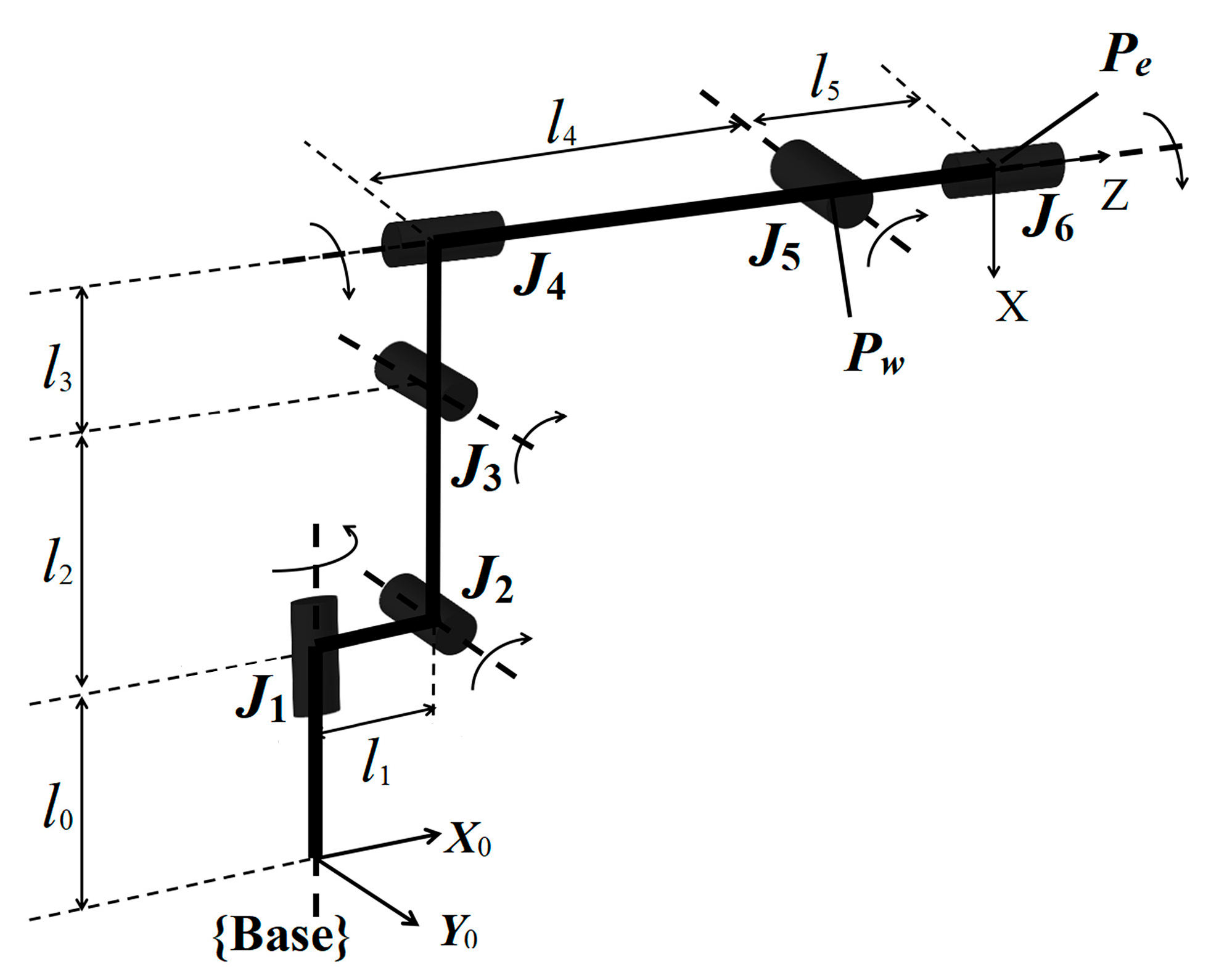
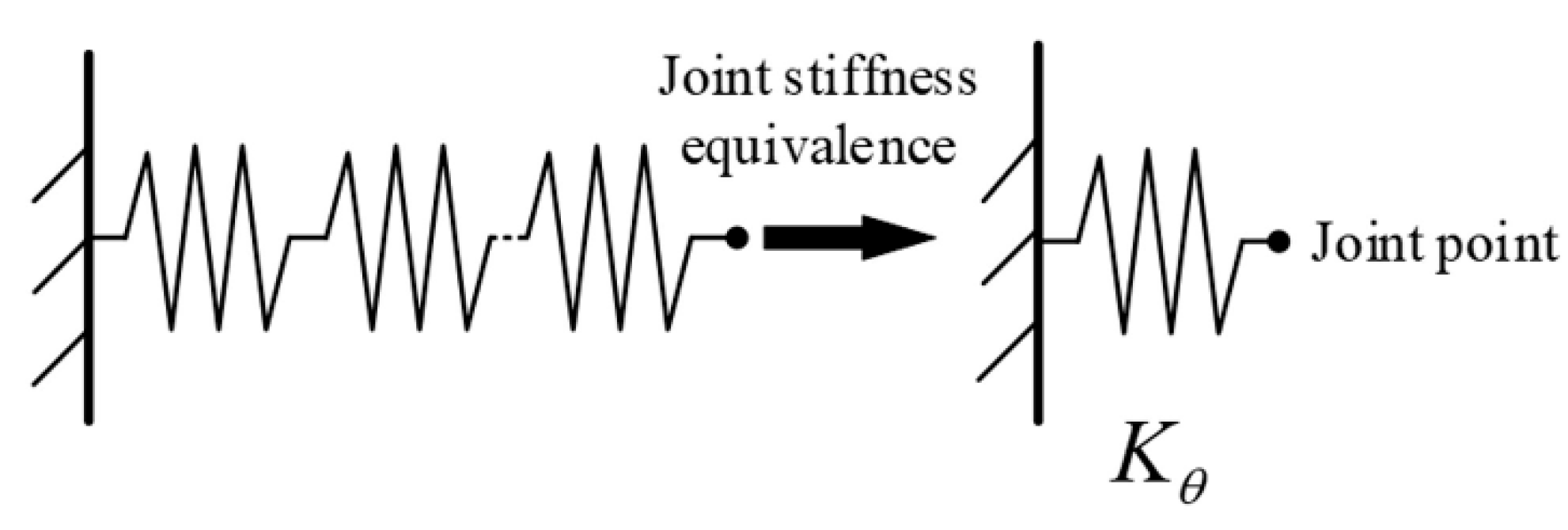
The drilling robot of the robot drilling system is a six-DOFs serial robot with a base connected to the ground. The robot joints are numbered from the base as J n ( n = 1, 2, 3, …, 6) and the links are numbered from the base as i ( i = 0, 1, 2, …,5), as shown in Figure 2. Using the virtual joint method, the power devices and transmission devices inside the robot joints such as motors, gears, chains, etc., are equivalent to springs with the stiffness of K θ as shown in Figure 3, where θ is the joint angular displacement.
Before modeling the stiffness of the robot, two assumptions are made according to the actual force and deformation of the drilling robot end during the machining process as follows:
(1) Assuming that the deformation of the robot is only caused by the external load when the robot is stable or is stationary;
(2) Assuming that the fourth link of the robot is a flexible body and the other five links are rigid bodies since the elastic deformations of the robot joints and the fourth link are the main sources of the robot deformation.
According to Equations (3) and (4) and the above assumption, the instantaneous motion of the robot end-effector V is expressed as
V = ω 6 v 6 = Q ^ 1 Q ^ 2 Q ^ 3 Q ^ 4 Q ^ 5 Q ^ 6 θ ˙ 1 θ ˙ 2 θ ˙ 3 θ ˙ 4 θ ˙ 5 θ ˙ 6
where ω 6 , v 6 is the three-dimensional angular velocity and linear velocity at the robot end, Q ^ i ( i = 1, 2, 3 …,6) represents the i -th joint movement of the robot and θ ˙ i is the i -th joint angular velocity.
The Jacobian matrix of the robot J ( θ ) can be expressed by dual quaternions as
J ( θ ) = Q ^ 1 Q ^ 2 Q ^ 3 Q ^ 4 Q ^ 5 Q ^ 6
According to the principle of virtual work, the external loads cause the generalized deformation of the robot end in the Cartesian space, and the work W ^ b performed by the robot end can be obtained as
W ^ b = s c ( F ^ · D ^ )
where s c ( ) represents the scalar part of the dual quaternion, F ^ is the external load at the robot end and D ^ is the displacement generated by F ^ at the robot end.
The work W ^ j performed by the robot in the joint space can be expressed as
W ^ j = s c ( i = 1 n q ^ τ i · δ ^ q i )
where q ^ τ i is the infinitesimal torque on the joint caused by the external load and δ ^ q i is the corresponding infinitesimal rotation angle.
The scalar sum of the real number and the dual part of W ^ b and W j ^ should be equal. This result can be expressed in matrix form as
τ q T d θ = T F T J d θ
where τ q T is the torque of the robot joint, T = [1 0 0 1 0 0] is the coefficient matrix and J is the Jacobian matrix of the robot. All matrices are in the form of quaternion.
According to the equivalent virtual spring, the joint stiffness matrix of the robot K θ can be expressed as
K θ = d i a g [ k θ 1 , k θ 2 , , k θ 6 ]
where k θ i ( i = 1, 2, …, 6) is the equivalent stiffness of the virtual spring of each joint.
According to Hooke’s law, the joint torque of the robot T q ^ can be expressed as
T q ^ = K θ · α
where α is the joint angular displacement of the robot.
When the external load F and the deformation X ^ at the robot end are small enough, the external load F can be expressed as
F = s c ( K ^ · X ^ )
where K ^ is the Cartesian stiffness matrix of the robot end in dual quaternion form.
Using Taylor’s expansion and ignoring higher-order infinitely small quantities, the external load F can be expressed as
F = K X
where K is the stiffness matrix of the robot end, F and X are 6 × 1 column vectors, and X is the deformation generated by the external load F at the robot end.
After derivation and transposition of Equation (9), combining Equations (11)–(13), the following can be obtained:
K ^ θ d θ = i = 1 6 J θ i d θ i F T T + J T K J d θ T T
According to Chen ‘s theory of the relationship between the torque on the end-effector and the joint torque [30], the inverse of the conservative congruence transformation (CCT) can be applied to simplify Equation (14). If the Jacobian matrix is invertible, its Moore–Penrose generalized inverse is used [31]. K can be expressed as
K = J T K θ K c J 1
where K c is the robot compensation stiffness matrix.
According to the research of Jian and Dumas [32], K c can be ignored when the Kinetostatic Conditioning Index (KCI) is greater than 0.45. Meanwhile, the experimental data with small errors can be obtained in the experiments of joint stiffness identification under this kind of posture. Equation (15) can be simplified as
K = J T K θ J 1
In order to improve the accuracy of the stiffness modeling, the deformation of the drilling robot link is considered. The fourth link, which is slender and prone to deformation compared to other links, is regarded as a flexible link, and is simplified as a simply supported beam with rigid joints and unilateral elastic constraints. According to the actual deformation of the robot during the drilling operation, the main deformation of the fourth link is lateral bending and twisting, and the unit stiffness matrix of the fourth link K J 4 can be expressed as
K J 4 = O ( u ) l 4 0 0 O ( u ) l 4 0 0 0 12 E I l 4 3 6 E I l 4 2 0 12 E I l 4 3 6 E I l 4 2 0 6 E I l 4 2 4 E I l 4 0 6 E I l 4 2 2 E I l 4 O ( u ) l 4 0 0 O ( u ) l 4 0 0 0 12 E I l 4 3 6 E I l 4 2 0 12 E I l 4 3 6 E I l 4 2 0 6 E I l 4 2 2 E I l 4 0 6 E I l 4 2 4 E I l 4
where E I is the bending stiffness, l 4 is the effective length of the fourth link, and O ( u ) is an infinitely small amount of displacement in direction of the link l 4 .
The stiffness matrix K E of the drilling robot considering the flexibility of the fourth link can be expressed as
K E = K K J 4

2.3. End-Effector Stiffness Modeling

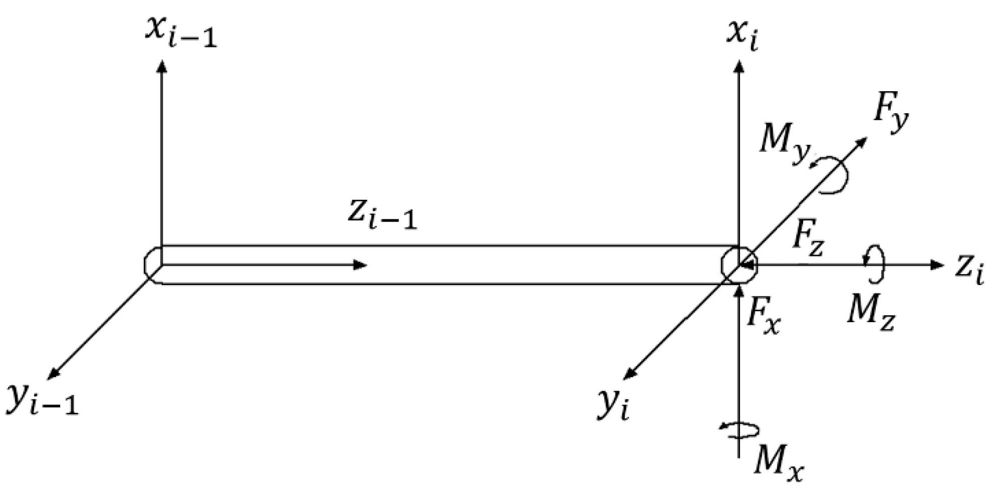
According to the Euler–Bernoulli beam theory, the end-effector can be simplified to a cantilever beam. It is assumed that the parts except for the cutting electric spindle and the drilling tool are rigid bodies, the material of the cantilever beam is isotropic, there is no eccentricity, the shear effect before and after deformation is not considered, and the end-effector conforms to the assumption of small deformation and small strain [33]. In order to analyze the stiffness of the cantilever beam, a coordinate system is established with the tool tip of the drilling tool as the origin, as shown in Figure 4.
The deformation of the cantilever beam in the x-axis direction caused by the force F x and bending moment M x are respectively x 1 and x 2 . The deformations of the cantilever beam in the y-axis direction caused by the force F y and bending moment M y are respectively y 1   and   y 2 . The deformations of the cantilever beam in the z-axis direction caused by the force F z and bending moment M z are respectively z 1 and z 2 .The stiffness matrix of the end-effector unit K E E can be expressed as
K E E = E A L 0 0 E A L 0 0 0 12 E I L 3 6 E I L 2 0 12 E I L 3 6 E I L 2 0 6 E I L 2 4 E I L 0 6 E I L 2 2 E I L E A L 0 0 E A L 0 0 0 12 E I L 3 6 E I L 2 0 12 E I L 3 6 E I L 2 0 6 E I L 2 2 E I L 0 6 E I L 2 4 E I L
where E I is the bending stiffness, E A is the tensile stiffness, and L is the length of the cantilever beam.
Since K E E is irreversible, the Moore–Penrose generalized inverse matrix K E E 1 [31] of the stiffness of the end-effector is expressed as
K E E 1 = a k E E 11 a k E E 16 a k E E 61 a k E E 66
where α k E E i j ( i = 1, 2, …, 6 and j = 1, 2, …, 6) is the element in the i -th row and j -th column of the Moore–Penrose generalized inverse matrix K E E 1 .

2.4. The Overall Stiffness Modeling of the Robot Drilling System

According to the linear superposition principle of the stiffness of the serial mechanism, the theoretical end deformation X t of the robot drilling system under the external load F can be expressed by the robot end deformation X E considering the flexibility of the fourth arm and the end-effector deformation X E E as
X t = K O 1 F = X E + X E E
where X E = K E 1 F , X E E = K E E 1 F , and K O 1 is the overall stiffness inverse matrix of the robot drilling system.
By combining Equations (6), (10), (16), (18) and (20), K O 1 can be expressed as
K O 1 = K E 1 + K E E 1 = K J 4 1 J   K θ 1 J T + K E E 1 = r 11 r 12 r 16 r 21 r 22 r 26 r 61 r 62 r 66
where r i j ( i = 1, 2, …, 6 and j = 1, 2, …, 6) is the element in the i -th row and j -th column of the overall stiffness inverse matrix K O 1 .
According to Equations (21) and (22), the theoretical end deformation considering the flexibility of the robot arm and end-effector in the robot drilling system can be expressed as
X t = ( K J 4 1 J   K θ 1 J T + K E E 1 ) F
It can be concluded that the theoretical end deformation of the robot drilling system is influenced by the robot postures, the flexibility of the robot arm and end-effector.

3. Experiments and Analysis

In order to verify the established stiffness model of the robot drilling system, the experimental setup is shown in Figure 5. The experimental setup is mainly composed of a drilling robot, an end-effector, the turnbuckle bolts and wire ropes, a force sensor, three dial indicators, and a drilling auxiliary workbench.
The ABB IRB-6700 industrial robot(ABB, Zurich, Switzerland) was applied as the drilling robot in the experimental setup, which features a rated payload capacity of 155 kg and an operational range of 2.6–3.2 m. The Denavit–Hartenberg (D-H) parameters of the drilling robot are listed in Table 1.
The robot end was connected to the high-speed cutting electric spindle as the end-effector. The drilling auxiliary workbench and the end-effector were connected by turnbuckle bolts and wire ropes, and the load was adjusted by the built-in lead screw of the turnbuckle bolts. The force sensor was connected to a data acquisition card to measure the external load F at the end-effector. A piezoelectric customized force sensor was applied for the load measurement of the end-effector and the three-axis orthogonal force components. The force sensor was installed between the robot end and the end-effector through the robot connection flange and integrated into the end-effector. The force sensor was installed in a centralized load transmission path, which can actually reflect the force at the end-effector of the drilling robot. The force sensor was calibrated pre-shipment with accuracy of ±0.1%, and a measuring range of 0–2000 N.
The load data acquisition was carried out using a USB data acquisition card, which has three channels configured to correspond to the voltage output of the force sensor in three directions. In the data acquisition, a linear conversion of voltage-to-force signal was performed based on the preset range. During the force loading process, due to the loosening of the screw of turnbuckle bolts, the received signal fluctuated within a certain range. The average of five measurements in the stable state segment was taken as the final measurement of the load.
The dial indicator with a measuring range of 0–10 mm and a measurement accuracy of ±0.010 mm was used to measure the actual end deformation X a of the robot drilling system. In the experimental setup, three sets of dial indicators were orthogonally integrated onto the measurement base via rigid rods, and their sensing axes were mutually perpendicular to form a Cartesian coordinate system. In the deformation measurement, five measurements were repeated for each test.
The experiments were conducted under controlled environmental conditions, with an ambient temperature of 20 ± 2 °C and an environmental vibration that the vibration velocity did not exceed 0.1 mm/s and vibration acceleration did not exceed 0.2 m/s2.
The applications of the experimental setup of the robot drilling system and the experiments aim to the drilling of workpiece of gray cast iron with tensile strength not less than 150 MPa and a hardness range of 150–220 HBS.
In the joint stiffness identification experiment, the actual end deformation X a of the robot drilling system measured by the dial indicator is based on the base coordinate system of the robot, while the reference frame of the force vector measured by the force sensor is its own coordinate system. For the convenience of calculation, the reference frame of the force sensor is converted to the base coordinate system of the robot, and the coordinate system conversion is expressed as
F   B a s e = Q ^ F l g B a s e · Q ^ S e n F l g · F S e n · Q ^ * S e n F l g · Q ^ * F l g B a s e
where F S e n = [ F x F y F z   0   0   0 ] T is the generalized external load in the coordinate system of the force sensor, F B a s e = [ f x f y f z m x m y m z ] T is the generalized external load in the base coordinate system of the robot and Q ^ F l g B a s e is the quaternion transformation from the base coordinate system of the robot to the coordinate system of the robot end flange. Q ^ S e n F l g is the quaternion transformation from the coordinate system of the robot end flange to the coordinate system of the force sensor, and Q ^ * F l g B a s e and Q ^ * S e n F l g are the conjugate quaternions of Q ^ F l g B a s e and Q ^ S e n F l g respectively.
According to the research results of Jian and Dumas [32], the robot compensation stiffness matrix K c can be ignored when KCI is greater than 0.45, and the force-deformation curves can be considered as linear relationship. Ten robotic postures with KCI greater than 0.45 were selected for the stiffness model identification. The load vector F B a s e = [ f x   f y   f z   m x   m y   m z ] T in base coordinate system, the actual end deformation X a = x a x x a y x a z 0 0 0 T and theoretical end deformation X t = x t x x t y x t z 0 0 0 T of the robot drilling system in the coordinate system of the force sensor are shown in Table 2 and Table 3.
Based on the solution method of the robot joint stiffness given by Hou [34] and Equation(10), the joint stiffness matrix of the drilling robot K θ = diag[2.61 × 10⁶ 9.37 × 10⁵ 6.58 × 10⁵ 9.20 × 10⁵ 4.43 × 10⁴ 2.74 × 10⁴] N · m / r a d . Combining Equations (13), (16), (18) and (22), the overall stiffness matrix of the robot drilling system K O can be further calculated.
K O is a 6×6 matrix that changes with the robot postures. In order to visually verify the accuracy of the calculation of K O , five postures were selected under the same experimental conditions, and three different loads were applied to each posture. The theoretical end deformation was calculated as X t (mm) according to Equation (23). The experimental data are shown in Table 3. From the actual and theoretical end deformation data in Table 3, the relative errors of end deformation ( ε x , ε y , ε z ) in the XYZ coordinate axes can be calculated as follows:
ε x = | x t x x a x x a x | × 100 % ε y = | x t y x a y x a y | × 100 % ε z = | x t z x a z x a z | × 100 %
The relative error of resultant end deformation ε d can be expressed as
ε d = | ( x t x ) 2 + ( x t y ) 2 + ( x t z ) 2 ( x a x ) 2 + ( x a y ) 2 + ( x a z ) 2 ( x a x ) 2 + ( x a y ) 2 + ( x a z ) 2 | × 100 %
To ensure the reliability of the experimental results, an uncertainty assessment was conducted on the measured values of the load vector and end deformation. Through statistical analysis of the load and end deformation data obtained from five repeated measurements under the same conditions, the standard deviation was used to determine the standard uncertainty of type A.
The force sensor was installed in a centralized load transmission path, which can actually reflect the force at the end-effector of the drilling robot. The deformation was directly measured by a dial indicator, and the error caused by the angle between the movement direction of the indicator probe and the coordinate axis direction is a second-order infinitesimal. The influence of environmental conditions on measurement results can be ignored, since the environment conditions were controlled. Therefore, the uncertainty of type B mainly comes from the accuracy of the measuring gauge, and the uncertainty of type B can be estimated by the accuracy of force sensor and dial indicator. The results of the measurement uncertainty for stiffness model validation are shown in Table 4.
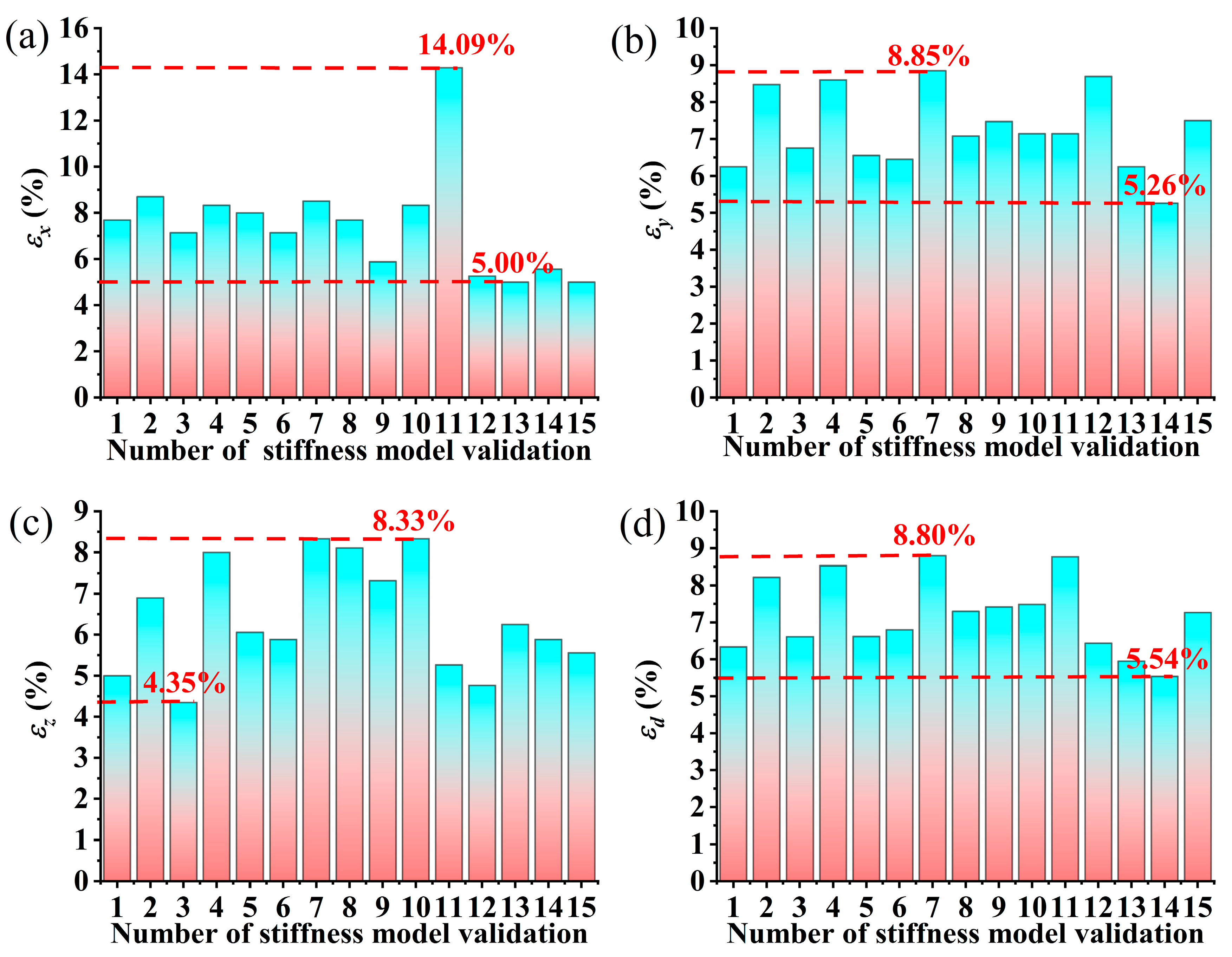
The results of relative errors of end deformation for stiffness model validation are shown in Figure 6.
In Figure 6, the maximum relative error of end deformation in the X-axis is 14.09%, the maximum relative error of end deformation in the Y-axis is 8.85% and the maximum relative error of end deformation in the Z-axis is 8.33%. The maximum relative error of resultant end deformation is 8.80%, the average relative error of resultant end deformation is 7.21% and the relative error of resultant end deformation is controlled within 10%. The experiment results show that this model is capable of predicting the deformation of the robotic drilling system.
The reasons for the error between the measured end deformation and the theoretical end deformation may be as follows:
(1) The arm parameters of the robot are different from theoretical parameters due to the different assembly and matching accessories of the robot drilling system;
(2) The self-weight of the robot in practical use causes the errors of the joint offset;
(3) Equipment wear.
The error from the environmental conditions can be ignored since the environmental conditions were controlled. In the stiffness modeling of industrial robots, incorporating the robot’s own weight requires the introduction of mass parameters and center of gravity positions for various components. This necessitates precise measurement or the calculation of the weight and center of gravity of each robot part, which increases the computational load of the modeling, such as coupled dynamic and static analysis, and may reduce real-time performance and place higher demands on algorithm efficiency.
The maximum relative error of this modeling method (8.80%) is significantly lower than the result reported by Chen et al. (10–15%) [35]. This performance improvement is mainly attributed to the fact that this model takes into account the flexibility of joints and links, thereby enhancing the accuracy of the modeling. By adopting the compact mathematical framework of dual quaternions, the derivation of the robot’s Jacobian matrix has been simplified. Meanwhile, the dual quaternions retain clear physical meaning and are superior to the purely numerical output of FEM. The current model has been verified for serial drilling robots, and when applied to more complex configurations, the kinematic mapping needs to be rederived. Although this model is limited by quasi-static loading conditions, its high accuracy in predicting static stiffness makes it an effective stiffness modeling tool for posture optimization of low-speed operations such as drilling in the fields of automotive and aerospace manufacturing.

4. Conclusions

In order to explore the suppressing method of the machining chatter mainly due to the low stiffness of the robot, a robot drilling workstation was constructed, including a drilling robot, a high-speed cutting electric spindle as the end-effector and an auxiliary workbench. A method was proposed for establishing the overall stiffness model of the robot drilling system, which combined the stiffness of the robot body and the end-effector using the linear superposition principle. Based on the virtual joint method and dual quaternion, the stiffness model was established by considering the flexibility of the robot arm. The stiffness model of the end-effector was built using the Euler–Bernoulli beam assumption. The experiment results show that the maximum relative error of resultant end deformation is 8.80%. This method provides an overall stiffness modeling of the robot drilling system, including the end-effector for stiffness modeling in suppressing the chatter caused by insufficient stiffness and a new approach of stiffness modeling for the intelligent manufacturing industry to overcome the problem of insufficient robot stiffness.

Author Contributions

Conceptualization, Y.-F.Z., B.-G.Y., G.T., Y.-X.G. and T.-F.N.; methodology, Y.-F.Z., B.-G.Y., G.T., Y.-X.G. and T.-F.N.; software, G.T. and Y.-X.G.; validation, Y.-F.Z., G.T., Y.-X.G. and F.Z.; formal analysis, B.-G.Y., Y.-X.G. and X.-F.L.; investigation, Y.-F.Z., G.T., Y.-X.G. and F.Z.; resources, B.-G.Y., F.Z. and X.-F.L.; data curation, B.-G.Y. and G.T.; writing—original draft preparation, Y.-F.Z., B.-G.Y., G.T. and Y.-X.G.; writing—review and editing, Y.-F.Z., B.-G.Y. and G.T.; visualization, B.-G.Y. and G.T.; supervision, B.-G.Y.; project administration, B.-G.Y. and F.Z.; funding acquisition, B.-G.Y., F.Z. and X.-F.L. All authors have read and agreed to the published version of the manuscript.

Funding

This research was funded by National Natural Science Foundation of China (Grant Nos. 52475578 and 32372007).

Data Availability Statement

The original contributions presented in the study are included in the article; further inquiries can be directed to the corresponding authors upon reasonable request.

Conflicts of Interest

The authors declare no conflicts of interest.

Abbreviations

The following abbreviations are used in this manuscript:
DOFDegrees-of-freedom
FEAFinite element analysis
MSAMatrix structure analysis
VJMVirtual joint method
CCTConservative congruence transformation
MBSMulti-body simulation method
IKInverse kinematic
KCIKinetostatic Conditioning Index
D-HDenavit–Hartenberg

References

  1. Wu, K.; Li, J.; Zhao, H.; Zhong, Y. Review of Industrial Robot Stiffness Identification and Modelling. Appl. Sci. 2022, 12, 8719. [Google Scholar] [CrossRef]
  2. Newman, M.; Khoshdarregi, M. Automatic Structural Identification and Vibration Suppression of Industrial Robots using a Custom Active Damper. In Proceedings of the 2022 22nd International Conference on Control, Automation and Systems (ICCAS), Jeju, Republic of Korea, 27 November 2022–1 December 2022; pp. 1033–1038. [Google Scholar] [CrossRef]
  3. Ozakyol, H.; Karaman, C.; Bingul, Z. Advanced robotics analysis toolbox for kinematic and dynamic design and analysis of high-DOF redundant serial manipulators. Comput. Appl. Eng. Educ. 2019, 27, 1429–1452. [Google Scholar] [CrossRef]
  4. Ji, W.; Wang, L. Industrial Robotic Machining: A Review. Int. J. Adv. Manuf. Technol. 2019, 103, 1239–1255. [Google Scholar] [CrossRef]
  5. Cordes, M.; Hintze, W.; Altintas, Y. Chatter stability in robotic milling. Robot. Comput. Int. Manuf. 2019, 55, 11–18. [Google Scholar] [CrossRef]
  6. Gao, Y.; Gao, H.; Bai, K.; Li, M.; Dong, W. A Robotic Milling System Based on 3D Point Cloud. Machines 2021, 9, 355. [Google Scholar] [CrossRef]
  7. Souflas, T.; Gerontas, C.; Bikas, H.; Stavropoulos, P. On the Optimization of Robot Machining: A Simulation-Based Process Planning Approach. Machines 2024, 12, 521. [Google Scholar] [CrossRef]
  8. Li, B.; Cui, G.; Tian, W.; Liao, W. Vibration suppression of an industrial robot with AGV in drilling applications by configuration optimization. Appl. Math. Model. 2022, 112, 614–631. [Google Scholar] [CrossRef]
  9. Zhao, X.; Zheng, L.; Shi, M.; Zhang, Y. Controlling harmful milling vibration for robotic milling system based on the optimization of milling posture and spindle speed. Proc. IMechE. Part B J. Eng. Manuf. 2024. [Google Scholar] [CrossRef]
  10. Doukas, C.; Pandremenos, J.; Stavropoulos, P.; Foteinopoulos, P.; Chryssolouris, G. On an Empirical Investigation of the Structural Behavior of Robots. Procedia CIRP 2012, 3, 501–506. [Google Scholar] [CrossRef]
  11. Marie, S.; Courteille, E.; Maurine, P. Elasto-geometrical modeling and calibration of robot manipulators: Application to machining and forming applications. Mech. Mach. Theory 2013, 69, 13–43. [Google Scholar] [CrossRef]
  12. Kermanian, A.; Kamali, E.A.; Taghvaeipour, A. Dynamic analysis of flexible parallel robots via enhanced co-rotational and rigid finite element formulations. Mech. Mach. Theory 2019, 139, 144–173. [Google Scholar] [CrossRef]
  13. Chen, D.; Song, A.; Ang, L.J. Design and Calibration of a Six-axis Force/torque Sensor with Large Measurement Range Used for the Space Manipulator. Procedia Eng. 2015, 99, 1164–1170. [Google Scholar] [CrossRef]
  14. Kouritem, S.A.; Abouheaf, M.I.; Nahas, N.; Hassan, M. A multi-objective optimization design of industrial robot arms. Alex. Eng. J. 2022, 61, 12847–12867. [Google Scholar] [CrossRef]
  15. Raoofian, A.; Taghvaeipour, A.; Kamali, E.A. On the stiffness analysis of robotic manipulators and calculation of stiffness indices. Mech. Mach. Theory 2018, 130, 382–402. [Google Scholar] [CrossRef]
  16. Cammarata, A. Unified formulation for the stiffness analysis of spatial mechanisms. Mech. Mach. Theory 2016, 105, 272–284. [Google Scholar] [CrossRef]
  17. Xu, H.; Xue, J.; Guo, G.; Liu, Y.; Liu, M.; Zhang, D. Stiffness Optimization of a Robotic Drilling System for Enhanced Accuracy in Aerospace Assembly. Actuators 2025, 14, 86. [Google Scholar] [CrossRef]
  18. Gosselin, C. Stiffness mapping for parallel manipulators. IEEE Trans. Robot. Autom. 1990, 6, 377–382. [Google Scholar] [CrossRef]
  19. Klimchik, A.; Pashkevich, A.; Caro, S.; Chablat, D. Stiffness Matrix of Manipulators with Passive Joints: Computational Aspects. IEEE Trans. Robot. 2012, 28, 955–958. [Google Scholar] [CrossRef]
  20. Dumas, C.; Caro, S.; Garnier, S.; Furet, B. Joint stiffness identification of six-revolute industrial serial robots. Robot. Comput. Int. Manuf. 2011, 27, 881–888. [Google Scholar] [CrossRef]
  21. Gorgulu, I.; Dede, M.; Kiper, G. Stiffness modeling of a 2-DoF over-constrained planar parallel mechanism. Mech. Mach. Theory 2023, 185, 105343. [Google Scholar] [CrossRef]
  22. Singh, A.; Padayachee, J.; Bright, G. An experimental approach to improve the joint stiffness of industrial robots through dexterous posture identification. South Afr. J. Ind. Eng. 2021, 32, 113–128. [Google Scholar] [CrossRef]
  23. Cao, W.; Ding, H. A method for stiffness modeling of 3R2T overconstrained parallel robotic mechanisms based on screw theory and strain energy. Precis. Eng. 2018, 51, 10–29. [Google Scholar] [CrossRef]
  24. Stavropoulos, P.; Gerontas, C.; Bikas, H.; Souflas, T. Multi-Body dynamic simulation of a machining robot driven by CAM. Procedia CIRP 2022, 107, 764–769. [Google Scholar] [CrossRef]
  25. Huynh, H.; Assadi, H.; Dambly, V.; Rivière-Lorphèvre, E.; Verlinden, O. Direct method for updating flexible multibody systems applied to a milling robot. Robot. Comput. Integr. Manuf. 2021, 68, 102049. [Google Scholar] [CrossRef]
  26. Li, G.; Zhang, F.; Fu, Y.; Wang, S. Kinematic calibration of serial robot using dual quaternions. Ind. Robot 2019, 46, 247–258. [Google Scholar] [CrossRef]
  27. Li, G.; Zhang, F.; Fu, Y.; Wang, S. Joint Stiffness Identification and Deformation Compensation of Serial Robots Based on Dual Quaternion Algebra. Appl. Sci. 2019, 9, 65. [Google Scholar] [CrossRef]
  28. Souflas, T.; Papaioannou, C.; Manitaras, D.; Gerontas, C.; Stavropoulos, P. In-process Detection of Low and High Frequency Chatter in Robot Machining. Procedia CIRP 2024, 130, 824–829. [Google Scholar] [CrossRef]
  29. Xu, P.; Yao, X.; Liu, S.; Wang, H.; Liu, K.; Senthil, K.; Lu, W.; Bi, G. Stiffness modeling of an industrial robot with a gravity compensator considering link weights. Mech. Mach. Theory 2021, 161, 104331. [Google Scholar] [CrossRef]
  30. Chen, S.F.; Kao, I. Conservative Congruence Transformation for Joint and Cartesian Stiffness Matrices of Robotic Hands and Fingers. Int. J. Rob. Res. 2000, 19, 835–847. [Google Scholar] [CrossRef]
  31. Klimczak, M.; Cecot, W. On Moore-Penrose Pseudoinverse Computation for Stiffness Matrices Resulting from Higher Order Approximation. Math. Probl. Eng. 2019, 2019, 5060397. [Google Scholar] [CrossRef]
  32. Dumas, C.; Caro, S.; Chérif, M.; Garnier, S.; Furet, B. Joint stiffness identification of industrial serial robots. Robotica 2011, 30, 649–659. [Google Scholar] [CrossRef]
  33. Qian, Z.; Zhang, D. Impact Dynamics of Multi-Link Robots with Link and Joint Flexibility. Appl. Mech. Mater. 2012, 226–228, 685–692. [Google Scholar]
  34. Qu, W.; Hou, P.; Yang, G.; Huang, G.; Yin, F.; Shi, X. Research on the Stiffness Performance for Robot Machining Systems. Hangkong Xuebao/Acta Aeronaut. 2013, 34, 2823–2832. [Google Scholar] [CrossRef]
  35. Chen, S.; Zhou, T.; Hu, T. Stiffness modeling and error compensation method of 6-DOF milling robot. Comput. Integr. Manuf. Syst. 2023, 29, 404–418. [Google Scholar] [CrossRef]
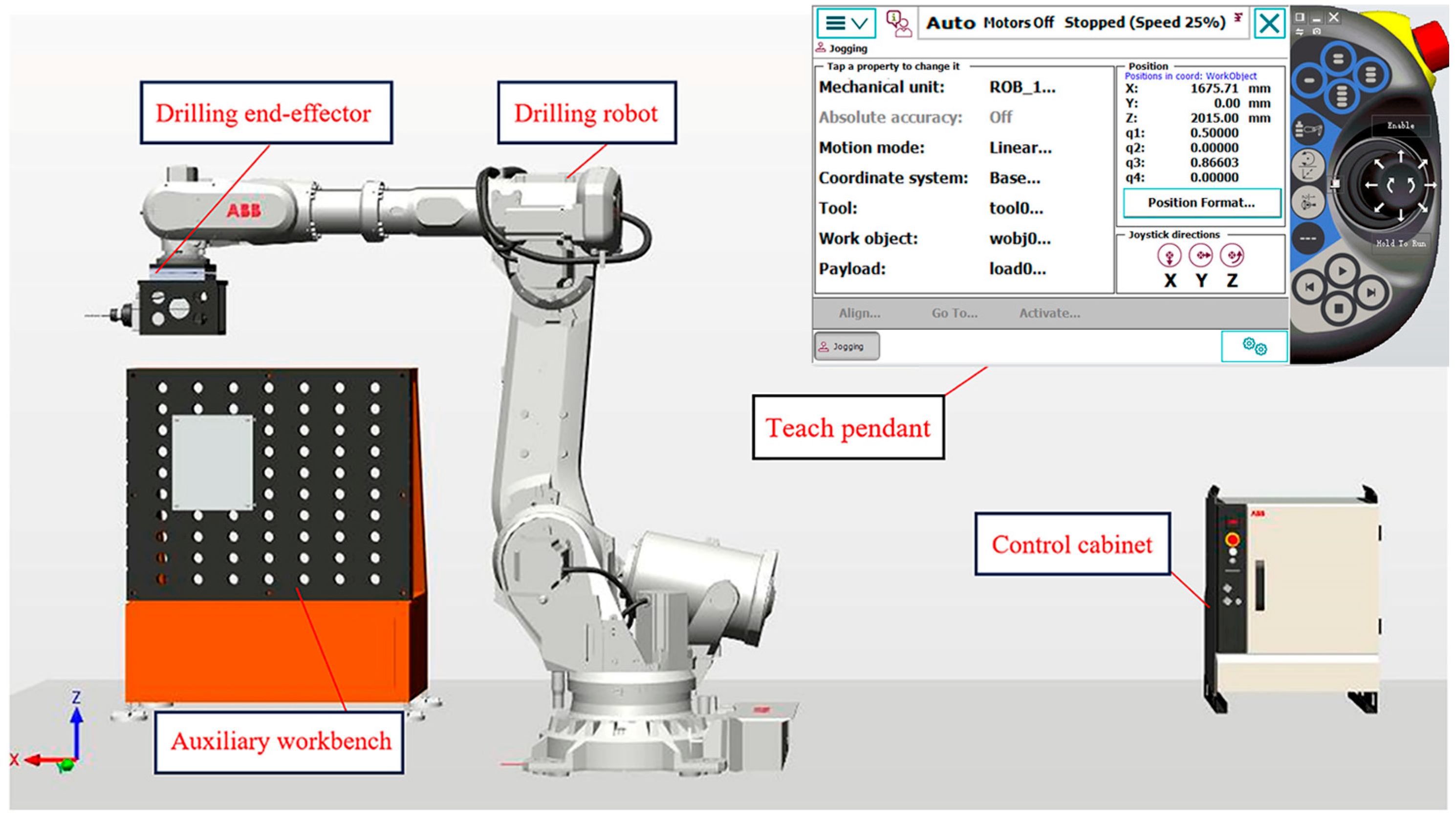
Figure 1. Workstation of the robot drilling system.
Machines 13 00837 g001
Figure 2. Schematic diagram of the robot link and joint.
Machines 13 00837 g002
Figure 3. Joint equivalent spring.
Machines 13 00837 g003
Figure 4. Coordinate system of end-effector cantilever beam.
Machines 13 00837 g004
Figure 5. Stiffness model verification experiment.
Machines 13 00837 g005
Figure 6. Results of relative end deformation error: (a) Relative end deformation error in X-axis ε x ; (b) relative end deformation in Y-axis ε y ; (c) relative end deformation error in Z-axis ε z ; (d) relative error of resultant end deformation ε d .
Machines 13 00837 g006
Table 1. The D-H parameters of the drilling robot.
Joint   No .   i Link   Length   a i 1 ( m m ) Joint   Torsion   Angle   α i 1 ( ° ) Joint   Angle   θ i ( ° ) Link   Offset   d i ( m m )
1 0 0 θ 1 780
2 320 90 θ 2 90 0
3 1125 0 θ 3 0
4 200 90 θ 4 1393
5 0 90 θ 5 0
6 0 90 θ 6 180 200
Table 2. Results of stiffness model identification.
PostureJoint Rotation Angle (°) Load   Vector   F B a s e (N, N, N, N·m, N·m, N·m) Actual   End   Deformation   ( x a x , x a y , x a z ) (mm)
1(0.69, −10.52, 46.04,
−1.15, −36.12, 182.16)
(1770.25, −778.50, 1133.60, −2.99 × 10⁵, −2.90 × 10⁵, −7.54 × 10⁵)(0.33, −1.28, −1.25)
(1610.98, −472.72, 892.64, −3.01 × 10⁴, 2.53 × 10⁵, −2.43 × 10⁵)(−0.15, −0.51, −0.13)
(1588.61, −673.75, 706.61, −8.67 × 10⁴, 6.11 × 10⁵, −6.24 × 10⁵)(−0.41, −1.32, −0.31)
2(2.48, 12.24, 20.30, 0.58, 57.02, 91.13)(2001.42, −218.76, 1170.64, 2.63 × 10⁴, −5.01 × 10⁵, 3.65 × 10⁵(−0.32, −0.83, −0.10)
(1846.22, −655.67, 792.49, −1.06 × 10⁵, 2.96 × 10⁵, −4.99 × 10⁵)(0.35, −1.31, 0.93)
(2068.95, −174.51, 915.41, 1.42 × 10⁵, −6.68 × 10⁴, 4.71 × 10⁵)(−0.37, −0.98, 0.28)
3(3.58, −19.55, 47.11, 0.54, 61.99, 92.30)(1718.11, −522.88, −48.82, −1.15 × 10⁵, −1.02 × 10⁵, −2.98 × 10⁵)(0.07, −0.56, −0.15)
(1673.29, −433.74, 1003.38, −4.53 × 10⁴, 9.50 × 10³, −1.49 × 10⁵)(0.06, −0.25, 0.11)
(1706.20, −467.53, 948.36, −4.65 × 10⁴, 9.17 × 10⁴, −1.99 × 10⁵)(0.10, −0.39, 0.26)
4(0.94, −13.23, 45.53, 182.69, 32.24, 0.80)(1708.22, −490.13, 1068.68, −1.02 × 10⁵, −1.33 × 10⁵, −2.41 × 10⁵)(0.18, −0.51, −0.60)
(1725.45, −565.85, 829.61, −6.44 × 10⁴, 3.01 × 10⁵, −3.76× 10⁵)(−0.34, −0.73, −0.62)
(1800.51, −657.77, 837.28, −1.23 × 10⁵, 2.47 × 10⁵, −5.20 × 10⁵)(−0.48, −0.92, −1.02)
5(6.45, −5.73, 56.42,
−0.01, 39.30, 6.45)
(2038.88, −177.64, 1023.05, 1.03 × 10⁵, −2.48 × 10⁵, 4.55 × 10⁵)(−1.12, −0.71, 0.58)
(1998.64, −160.10, 931.37, 1.46 × 10⁵, −5.38 × 10⁴, 4.73 × 10⁵)(0.63, −0.85, 0.57)
(1878.51, −56.16, 780.87, 2.61 × 10⁵, 2.98 × 10⁵, 6.24 × 10⁵)(0.29, −0.85, 0.44)
6(169.13, −34.85, −168.16, −2.24, −68.34, 174.59)(1753.28, −324.17, 1011.00, 1.84 × 10⁴, −5.31 × 10⁴, 8.28 × 10⁴)(0.44, −0.14, 0.32)
(1684.76, −321.17, 985.54, 2.91 × 10⁴, 3.57 × 10⁴, 6.44 × 10⁴)(−0.15, −0.05, 0.21)
(1696.50, −300.85, 953.10, 5.28 × 10⁴, 8.88 × 10⁴, 1.06 × 10⁵)(0.20, −0.17, 0.29)
7(168.12, −29.40, −176.2 6, −1.38, −67.99, 78.67)(1636.90, −267.16, 960.01, 7.07 × 10⁴, 1.12 × 10⁵, 1.48 × 10⁵)(0.25, −0.11, 0.18)
(1675.84, −221.22, 980.08, 9.15 × 10⁴, 5.13 × 10⁴, 2.47 × 10⁵)(0.21, −0.04, 0.36)
(1631.69, −181.80, 860.59, 1.57 × 10⁵, 3.00 × 10⁵, 3.04 × 10⁵)(0.50, −0.37, 0.43)
8(169.53, −37.18, −164.63, −1.26, −67.15, 257.83)(1796.83, −251.28, 901.44, 1.01 × 10⁵, 1.24 × 10⁵, 2.33 × 10⁵)(−0.21, −0.43, 0.35)
(1639.75, −369.52, 943.39, 1.46 × 10⁴, 1.41 × 10⁵, −4.11 × 10⁴)(0.15, −0.28, 0.26)
(1639.30, −485.30, 908.94, −4.34 × 10⁴, 2.05 × 10⁵, −2.56 × 10⁵)(0.94, −0.73, 0.56)
9(168.07, −34.74, −177.73, −1.45, −61.99, 168.82)(1888.07, −199.11, 839.03, 1.54 × 10⁵, 1.85 × 10⁵, 3.62 × 10⁵)(0.87, −0.29, 0.36)
(1753.77, −238.39, 872.75, 1.19 × 10⁵, 2.03 × 10⁵, 2.42 × 10⁵)(0.20, −0.21, 0.53)
(1850.06, −299.35, 981.58, 4.37 × 10⁴, −5.71 × 10⁴, 1.63 × 10⁵)(0.27, −0.06, 0.40)
10(168.52, −39.09, −161.67, −1.30, −71.95, −11.03)(1347.98, −374.87, 925.40, 1.76 × 10⁴, 3.51 × 10⁵, −1.53 × 10⁵)(0.69, −0.51, 0.44)
(1384.50, −360.66, 909.98, 3.16 × 10⁴, 3.58 × 10⁵, −1.14 × 10⁵)(0.62, −0.42, 0.47)
(1489.67, −329.45, 892.74, 5.66 × 10⁴, 3.26 × 10⁵, −1.93 × 10⁴)(0.44, −0.32, 0.52)
Table 3. Results of stiffness model validation.
Posture Load   Vector   F B a s e
(N, N, N, N·m, N·m, N·m)
Actual End Deformation Value ( x a x , x a y , x a z ) (mm)Theoretical End Deformation Value ( x t x , x t y , x t z ) (mm)Relative End Deformation Error ( ε x , ε y , ε z ) (%)
1(1530.16, −454.39, 1090.01, −8.82 × 10⁴, −6.46 × 10⁴, −2.37 × 10⁵)
(1414.39, −511.27, 1096.12, −1.25 × 10⁵, −5.88 × 10³, −3.83 × 10⁵)
(1669.30, −364.78, 1122.40, −4.52 × 10⁴, −2.09 × 10⁵, −2.20 × 10⁴)
(−0.26, −0.64, −0.20)
(−0.23, −0.59, −0.29)
(−0.28, −0.74, −0.23)
(−0.24, −0.60, −0.19)
(−0.21, −0.54, −0.27)
(−0.26, −0.69, −0.22)
(7.69, 6.25, 5.00)
(8.70, 8.47, 6.90)
(7.14, 6.76, 4.35)
2(1622.84, 549.23, 812.21, 2.88 × 10⁵, 3.95 × 10⁵, 6.49 × 10⁵)
(1811.02, −158.42, 864.27, 1.70 × 10⁵, 1.84 × 10⁵, 4.11 × 10⁵)
(1788.64, −266.74, 988.35, 6.11 × 10⁴, −3.24 × 10⁴, 2.02 × 10⁵)
(−0.36, −0.93, −0.25)
(−0.25, −0.61, 0.33)
(0.42, −0.31, 0.17)
(−0.33, −0.85, −0.23)
(−0.23, −0.57, 0.31)
(0.39, −0.29, 0.16)
(8.33, 8.60, 8.00)
(8.00, 6.56, 6.06)
(7.14, 6.45, 5.88)
3(1508.01, −79.93, 965.83, 1.82 × 10⁵, 1.79 × 10⁵, 4.50 × 10⁵)
(1457.17, −20.77, 1067.37, 1.82 × 10⁵, 2.16 × 10⁴, 5.42 × 10⁵)
(1607.32, −120.16, 892.32, 1.83 × 10⁵, 2.56 × 10⁵, 4.10 × 10⁵)
(−0.47, −1.13, 0.12)
(−0.65, −1.13, −0.37)
(−0.17, −1.07, −0.41)
(−0.43, −1.03, 0.11)
(−0.60, −1.05, −0.34)
(−0.16, −0.99, −0.38)
(8.51, 8.85, 8.33)
(7.69, 7.08, 8.11)
(5.88, 7.48, 7.32)
4(1527.92, −415.79, 927.15, −7.74× 10³, 2.39 × 10⁵, −1.66 × 10⁵)
(1603.52, −306.89, 916.25, 6.20 × 10⁴, 2.13 × 10⁵, 6.24 × 10⁴)
(1625.42, −371.78, 981.66, 1.63 × 10³, −3.72 × 10², 9.82 × 10²)
(−0.24, −0.42, 0.12)
(0.28, −0.42, −0.19)
(0.19, −0.23, −0.21)
(−0.22, −0.39, 0.11)
(0.24, −0.39, −0.18)
(0.18, −0.21, −0.20)
(8.33, 7.14, 8.33)
(14.29, 7.14, 5.26)
(5.26, 8.70, 4.76)
5(1607.13, −454.34, 943.38, −3.68 × 10⁴, 1.61 × 10⁵, −2.10 × 10⁵)
(1623.55, −669.43, 925.26, −1.61 × 10⁵, 1.85 × 10⁵, −6.03 × 10⁵)
(1641.85, −611.41, 848.49, −9.86 × 10⁴, 3.16 × 10⁵, −4.89 × 10⁵)
(0.20, −0.32, −0.16)
(−0.18, −0.19, −0.17)
(−0.20, −0.80, −0.18)
(0.19, −0.30, −0.15)
(−0.17, −0.18, −0.16)
(−0.19, −0.74, −0.17)
(5.00, 6.25, 6.25)
(5.56, 5.26, 5.88)
(5.00, 7.50, 5.56)
Table 4. Results of measurement uncertainty in stiffness model validation.
PostureStandard Uncertainty of Type A for Load in (x,y,z) of Base
(N, N, N)
Estimated Uncertainty of Type B for Load in (x,y,z) of Base
(N, N, N)
Standard Uncertainty of Type A for End Deformation in (x,y,z) (mm)Estimated Uncertainty of Type B for End Deformation in (x,y,z) (mm)
1(0.282, 0.153, 0.282)
(0.532, 0.217, 0.333)
(0.379, 0.355, 0.571)
(0.883, 0.262, 0.629)
(0.817, 0.295, 0.633)
(0.964, 0.211, 0.648)
(0.0054, 0.0073, 0.0018)
(0.0036, 0.0075, 0.0052)
(0.0057, 0.0082, 0.0022)
0.0069
2(0.788, 0.283, 0.433)
(0.527, 0.065, 0.279)
(0.338, 0.095, 0.398)
(0.937, 0.317, 0.469)
(1.046, 0.091, 0.499)
(1.033, 0.154, 0.571)
(0.0049, 0.0083, 0.0044)
(0.0028, 0.0066, 0.0063)
(0.0067, 0.0054, 0.0040)
0.0069
3(0.564, 0.033, 0.328)
(0.368, 0.012, 0.287)
(0.257, 0.055, 0.230)
(0.871, 0.046, 0.558)
(0.841, 0.012, 0.616)
(0.928, 0.069, 0.515)
(0.0059, 0.0100, 0.0018)
(0.0080, 0.0108, 0.0046)
(0.0022, 0.0091, 0.0073)
0.0069
4(0.413, 0.102, 0.377)
(0.442, 0.166, 0.349)
(0.430, 0.184, 0.411)
(0.882, 0.240, 0.535)
(0.926, 0.177, 0.529)
(0.938, 0.215, 0.567)
(0.0036, 0.0061, 0.0022)
(0.0066, 0.0052, 0.0033)
(0.0044, 0.0018, 0.0059)
0.0069
5(0.464, 0.221, 0.272)
(0.410, 0.343, 0.336)
(0.382, 0.183, 0.221)
(0.928, 0.262, 0.545)
(0.937, 0.386, 0.534)
(0.948, 0.353, 0.490)
(0.0052, 0.0061, 0.0046)
(0.0028, 0.0018, 0.0036)
(0.0033, 0.0098, 0.0057)
0.0069
Disclaimer/Publisher’s Note: The statements, opinions and data contained in all publications are solely those of the individual author(s) and contributor(s) and not of MDPI and/or the editor(s). MDPI and/or the editor(s) disclaim responsibility for any injury to people or property resulting from any ideas, methods, instructions or products referred to in the content.