Reinforcement Learning-Based Finite-Time Sliding-Mode Control in a Human-in-the-Loop Framework for Pediatric Gait Exoskeleton

Abstract

Rehabilitation devices such as actuated lower-limb exoskeletons can provide essential mobility assistance for pediatric patients with gait impairments. Enhancing their control systems under conditions of user variability and dynamic disturbances remains a significant challenge, particularly in active-assist modes. This study presents a human-in-the-loop control architecture for a pediatric lower-limb exoskeleton, combining outer-loop admittance control with robust inner-loop trajectory tracking via a non-singular terminal sliding-mode (NSTSM) controller. Designed for active-assist gait rehabilitation in children aged 8–12 years, the exoskeleton dynamically responds to user interaction forces while ensuring finite-time convergence under system uncertainties. To enhance adaptability, we augment the inner-loop control with a twin delayed deep deterministic policy gradient (TD3) reinforcement learning framework. The actor–critic RL agent tunes NSTSM gains in real-time, enabling personalized model-free adaptation to subject-specific gait dynamics and external disturbances. The numerical simulations show improved trajectory tracking, with RMSE reductions of 27.82% (hip) and 5.43% (knee), and IAE improvements of 40.85% and 10.20%, respectively, over the baseline NSTSM controller. The proposed approach also reduced the peak interaction torques across all the joints, suggesting more compliant and comfortable assistance for users. While minor degradation is observed at the ankle joint, the TD3-NSTSM controller demonstrates improved responsiveness and stability, particularly in high-load joints. This research contributes to advancing pediatric gait rehabilitation using RL-enhanced control, offering improved mobility support and adaptive rehabilitation outcomes.

1. Introduction

Gait impairments, often arising from neurological conditions such as cerebral palsy, spinal cord injury, or stroke, affect millions of individuals globally, significantly reducing their mobility and quality of life [1,2]. These conditions are particularly challenging in pediatric populations, where the rapid changes in anthropometric parameters complicate rehabilitation efforts [3]. Traditional therapeutic interventions, although effective, rely heavily on manual assistance, which is labor-intensive, costly, and difficult to scale [4]. Consequently, robotic rehabilitation devices like lower-limb exoskeletons (LLEs) have emerged as transformative solutions for delivering repetitive task-oriented training that is essential for motor recovery [5,6]. LLEs offer two main assistance modes: passive assistance (PA), which uses position/trajectory control to drive limb motion, and active assistance (AA), which combines user muscle effort with admittance or impedance control—suitable for patients with residual limb strength.

While passive-assisted LLERs have been widely studied [7], position control alone is inadequate for AA modes where patient muscle participation is essential. This has led to growing interest in combining admittance or impedance control with trajectory control, referred to as human-in-the-loop control, to promote active user involvement. Early work in [8] introduced a method of generalized elasticities to diminish the interaction forces. However, the interaction forces should not be minimized in the case of AA training mode to increase the varying forms of assistance by the user. The researchers in [9] presented a patient-human-in-the-loop control strategy for a single-degree-of-freedom (1-DOF) lower-limb exoskeleton system in which the dynamics of impedance is controlled using fuzzy logic, specifically aimed at reducing the interaction forces at the points of contact with the user. The researchers in [10] introduced a fuzzy logic admittance control system for a 2-DOF ankle therapeutic device with varying levels of assistance or resistance. In related research on human-in-the-loop control, Chen et al. [11] introduced an adaptive impedance control strategy to enable AA, using a disturbance observer to estimate interaction forces under cost constraints. More recently, Mosconi et al. [12] conducted simulations to evaluate the effectiveness of impedance control in supporting lower-limb impairments during the swing phase.

Despite the human-in-the-loop control promise, exoskeleton control remains challenging due to nonlinear system dynamics, user variability, and unpredictable external disturbances such as involuntary muscle contractions [3,13]. Conventional trajectory feedback controllers like PD and PID are easy to implement but often fail under significant parameter variations or perturbations [3]. Model-based strategies such as computed torque control (CTC) and sliding-mode control (SMC) offer robustness against uncertainties but typically rely on accurate system models and meticulous gain tuning. Recent examples include hierarchical torque control for active assistance [14], time-delay robust CTC [15], and adaptive SMC variants using fuzzy logic [16], radial basis function compensators [17], and fast terminal sliding modes for sit-to-stand transitions [18]. While these methods have achieved high tracking performance in simulations and early prototypes, a shared limitation is their dependence on accurate modeling and manually tuned parameters.

To address this, reinforcement learning (RL) has gained traction as a model-free approach to adaptive control. Unlike classical controllers, RL enables agents to learn optimal policies directly from environment interactions, making it particularly valuable in human–exoskeleton systems where dynamics are uncertain and user-specific. Deep reinforcement learning (DRL), which uses neural networks as function approximators, has shown promise in continuous high-dimensional control tasks characteristic of lower-limb rehabilitation robotics. Early studies applied Q-learning and DDPG for mapping sensory inputs to control torques [19,20], while more recent efforts have used Proximal Policy Optimization (PPO) to dynamically adjust assistance levels [21] and achieve robustness via domain randomization.

Hybrid control frameworks that combine the robustness of SMC with the adaptability of DRL have recently emerged as powerful alternatives. For instance, Hfaiedh et al. [22] used a DDPG approach to adapt a non-singular terminal SMC for upper-limb exoskeleton control, achieving improved tracking and disturbance resilience. Similarly, Khan et al. [23] integrated SMC with an Extended State Observer and DDPG to enhance multibody robot tracking, outperforming optimal PID and H-infinity controllers. Zhu et al. [24] used PPO to tune a terminal SMC controller online, improving robustness to matched and mismatched disturbances. Notably, TD3 has become a preferred actor–critic algorithm in such contexts due to its delayed policy updates and clipped double-Q estimation, which mitigate overestimation bias and improve learning stability [25,26]. A notable example is the work by Sun et al. [27], who proposed a reinforcement learning framework for soft exosuits that combines a conventional PID controller with a learned policy. This approach enables the system to adaptively modify assistive torques in response to user-specific gait variations, demonstrating improved performance and wearer comfort in both simulations and physical trials. Similarly, Li et al. [28] applied TD3 to augment an active disturbance-rejection controller (ADRC) for lower-limb exoskeletons, achieving enhanced tracking and disturbance rejection in both simulated and experimental settings. These hybrid designs often outperform standalone SMC, PID, or neural approaches, especially under uncertainty and parameter drift [29].

Building on these promising advances, further research is needed to translate hybrid DRL–model-based control frameworks into practical human-in-the-loop systems for pediatric gait rehabilitation. In AA modes, inner-loop controllers must not only provide robust trajectory tracking under disturbances and user variability but should also adapt safely and effectively to joint-specific dynamics and subject-specific behaviors. Achieving real-time gain adaptation in such nonlinear human-interactive systems remains challenging, particularly given the safety-critical nature of pediatric applications and the need to balance responsiveness with stability. Motivated by these challenges, this work proposes a novel human-in-the-loop control framework that integrates outer-loop admittance control with a TD3-tuned finite-time NSTSM inner-loop controller for gait tracking in pediatric exoskeletons. The key contributions are as follows:

(i)

We introduce human-in-the-loop control with admittance control in the outer loop and finite-time sliding-mode control in the inner loop, improving robustness without requiring precise modeling of a pediatric exoskeleton system.

(ii)

We introduce a TD3-based DRL approach to tune and adjust the gains of the NSTSM controller (TD3-NSTSM) online in the human-in-the-loop control.

(iii)

We test the proposed human-in-the-loop control numerically for a gait trajectory of a healthy pediatric participant of age 12 years.

(iv)

We compare the admittance control performance of the baseline NSTSM with that of the TD3-tuned admittance using standard tracking metrics: maximum absolute deviation (MAD), root mean square error (RMSE), and integral of absolute error (IAE).

2. Exoskeleton Setup, Parameters, and Dynamic Modeling

2.1. Exoskeleton Setup and Parameters

The structural integrity and stability of the exoskeleton are critical considerations in its design. This entails ensuring that the exoskeleton can withstand various static and dynamic forces. Furthermore, the exoskeleton must incorporate the required degrees of freedom (DOFs) to prioritize the user’s safety. A significant drawback of current pediatric exoskeletons is their limited structural stability. To address this, the proposed RL-augmented finite-time control approach is applied to a stand-supported lower-limb exoskeleton designed for pediatric gait rehabilitation, aiming to enhance balance and stability during overground gait training. Considering the specified design requirements, Narayan et al. [3] introduced a 6-DOF stand-aided exoskeleton robot (LLES v2) aimed at pediatric gait rehabilitation. It is specifically designed for children aged 8–12 years with a body weight of 25–40 kg and a consistent height of 130 ± 2 cm. The design incorporates three active joints in the sagittal plane to facilitate lower-limb movements: hip flexion/extension (f/e), knee flexion/extension (f/e), and ankle dorsiflexion/plantarflexion (d/p). Figure 1a–c provides an overview of the CAD model of the LLES v2. To ensure user safety, the maximum range of motion (ROM) for each lower-limb joint is set as follows: 30°/−12° for hip (f/e), 60°/−10° for knee (f/e), and 13°/−20° for ankle (d/p).

Table 1. Labeled components of the LLES v2 exoskeleton as shown in Figure 1.

Label	Component Description
Exoskeleton Limbs (Figure 1a)
1	Thigh segment
2	Shank segment
3	Foot segment
4	Hybrid stepper motor
5	Lead screw actuator
6	Extended shank segment
7	Lead screw mechanism
8	Stepper motor
9	Supporting splints
10	Coupling element
Fully Assembled System (Figure 1b)
1	Base frame
2	Wheel-mounted support

Table 1. Labeled components of the LLES v2 exoskeleton as shown in Figure 1.

Label	Component Description
Exoskeleton Limbs (Figure 1a)
1	Thigh segment
2	Shank segment
3	Foot segment
4	Hybrid stepper motor
5	Lead screw actuator
6	Extended shank segment
7	Lead screw mechanism
8	Stepper motor
9	Supporting splints
10	Coupling element
Fully Assembled System (Figure 1b)
1	Base frame
2	Wheel-mounted support

The breakdown of lower-limb parameters for the pediatric participant and the exoskeleton is summarized in

Table 2. Specifications of LLES v2 and human child.

	Part	Mass (kg)	Length (m)	COM (m)
LLES	Thigh link	$m_{1e}$ = 4.55	$l_{1e}$ = 0.30	$l_{c1e}$ = 0.15
	Shank link	$m_{2e}$ = 1.70	$l_{2e}$ = 0.28	$l_{c2e}$ = 0.14
	Foot link	$m_{3e}$ = 0.75	$l_{3e}$ = 0.08	$l_{c3e}$ = 0.04
Child (12 yrs)	Thigh	$m_{1h}$ = 4.40	$l_{1h}$ = 0.28	$l_{c1h}$ = 0.14
	Shank	$m_{2h}$ = 2.12	$l_{2h}$ = 0.28	$l_{c2h}$ = 0.14
	Foot	$m_{3h}$ = 0.84	$l_{3h}$ = 0.05	$l_{c3h}$ = 0.02

. The parameters of the exoskeleton system, such as mass and length, were determined using the SolidWorks 2021 model [3]. Conversely, the masses of the lower-limb segments for the human participant were estimated based on the well-established anatomical research conducted by Jensen [30]. The segment lengths for the human subject were directly measured with a tape and further validated using a Kinect-LabVIEW-based motion capture (MOCAP) system. The desired joint and Cartesian trajectories for a 12-year-old male child (body mass: 40 kg; height: 132 cm) were derived using the MOCAP system, with its methodology detailed in Narayan and Dwivedy [31]. The recorded ranges of motion (ROMs) for the hip, knee, and ankle joints of the child were 22.23° to −8.93°, 58.21° to 1.15°, and 5.18° to −7.96°, respectively.

2.2. Dynamic Modeling

To determine the functional joint torques in a human–exoskeleton system, dynamic modeling is essential. The exoskeleton robot must coordinate its joint movements with the human user and enable effective physical interaction. This study incorporates physical interaction by developing a dynamic model of the combined human–exoskeleton system. A three-link structure resembling the human lower limb is considered Figure 2a, and the system’s behavior is modeled using the Euler–Lagrange approach [32,33] to derive the state-space equations.

$$\begin{array}{cc}\hfill {\tau }_{i,h}& =M_h\left(q_{i,h}\right){\ddot{q}}_{i,h}+C_h\left(q_{i,h},{\dot{q}}_{i,h}\right){\dot{q}}_{i,h}+G_h\left(q_{i,h}\right)\hfill \end{array}$$

(1)

$$\begin{array}{cc}\hfill {\tau }_{i,e}& =M_e\left(q_{i,e}\right){\ddot{q}}_{i,e}+C_e\left(q_{i,e},{\dot{q}}_{i,e}\right){\dot{q}}_{i,e}+G_e\left(q_{i,e}\right)\hfill \end{array}$$

(2)

The terms h and e denote human and exoskeleton robot, and $i($=$1,2,3)$ represents the hip, knee, and ankle joint, respectively. The variables ${\tau }_{i,h}$ and ${\tau }_{i,e}$ indicate the torque inputs applied at the joints of the human and the exoskeleton, respectively. The vectors $q_{i,h}$ and $q_{i,e}$ describe the joint positions (i.e., angular states) for the human and exoskeleton systems, whereas ${\dot{q}}_{i,h}$ and ${\dot{q}}_{i,e}$ represent the corresponding joint velocities. The second derivatives, ${\ddot{q}}_{i,h}$ and ${\ddot{q}}_{i,e}$, capture joint accelerations for both entities. The terms $M_h\left(q_{i,h}\right)\in {\mathbb{R}}^{3\times 3}$ and $M_e\left(q_{i,e}\right)\in {\mathbb{R}}^{3\times 3}$ define the inertia matrices for the human and exoskeleton systems and are symmetric and positive definite. Similarly, the matrices $C_h(q_{i,h},{\dot{q}}_{i,h})$ and $C_e(q_{i,e},{\dot{q}}_{i,e})$, both in ${\mathbb{R}}^{3\times 3}$, encapsulate the Coriolis and centrifugal force terms arising from motion dynamics. Finally, the gravitational influences acting on the joints are denoted by $G_h\left(q_{i,h}\right)$ and $G_e\left(q_{i,e}\right)$, each in ${\mathbb{R}}^3$. Detailed formulations of these mass, velocity-dependent, and gravity-related components can be found in [34].

The stiffness of bracing pads makes interaction forces in PA mode seem insignificant. In contrast, AA mode captures flexible interactions by permitting relative motion between the exoskeleton and the human leg. While sensors measure interaction forces in real setups, simulations often approximate them using viscoelastic (spring-damper) models [35,36,37]. To depict compliant connections at the thigh, shank, and ankle–foot between the human (red) and exoskeleton (blue), three linear Voigt models are used, as shown in Figure 2b.

$${\tau }_{i,\mathrm{int}}=c\left({\dot{q}}_{i,e}-{\dot{q}}_{i,h}\right)+k\left(q_{i,e}-q_{i,h}\right)$$

(3)

Here, $\left({\dot{q}}_{i,e}-{\dot{q}}_{i,h}\right)$ and $\left(q_{i,e}-q_{i,h}\right)$ are the differences in angular velocity and position for the ith joint, with c representing the damping coefficient and k representing the spring coefficient of the bracing pads.

Additionally, it is worth acknowledging that the actual behavior of an exoskeleton robot often deviates from its mathematical model due to uncertainties in parameters and unexpected external influences. To account for these differences, the dynamic equation of the exoskeleton (Equation (2)) is revised accordingly.

$$\begin{array}{cc}\hfill {\tau }_{i,e}-{\tau }_{i,int}+{\tau }_d=& \left(M_{oe}\left(q_{i,e}\right)+\delta M_e\left(q_{i,e}\right)\right){\ddot{q}}_{i,e}+\left(C_{oe}\left(q_{i,e},{\dot{q}}_{i,e}\right)+\delta C_e\left(q_{i,e},{\dot{q}}_{i,e}\right)\right){\dot{q}}_{i,e}\hfill \\ \hfill & +\left(G_{oe}\left(q_{i,e}\right)+\delta G\left(q_{i,e}\right)\right)+F\left({\dot{q}}_{i,e}\right)\hfill \end{array}$$

(4)

where ${\tau }_d\in {\mathbb{R}}^3$ is the disturbance vector; $M_{\mathrm{oe}}\in {\mathbb{R}}^{3\times 3},C_{\mathrm{oe}}\in {\mathbb{R}}^{3\times 3}$, and $G_{\mathrm{oe}}\in {\mathbb{R}}^3$ denote the inertia, Coriolis, and gravity matrix with nominal values, respectively; $\delta$ is the uncertain scaling factor; and $F\left({\dot{q}}_{i,e}\right)\in {\mathbb{R}}^3$ is the friction effect of the Coulomb friction $C_f\in {\mathbb{R}}^3$ and viscous friction $V_f\left(=\sigma {\dot{q}}_{i,e}\right)\in {\mathbb{R}}^3$, as mentioned as follows [38]

$$F\left({\dot{q}}_{i,e}\right)={\mathrm{C}}_f\mathrm{sgn}\left({\dot{q}}_{i,e}\right)+V_F={\mathrm{C}}_f\mathrm{sgn}\left({\dot{q}}_{i,e}\right)+\sigma \left({\dot{q}}_{i,e}\right)$$

(5)

Here, $\sigma$ represents the parameter for angular velocity, expressed in $\mathrm{Nm}/{\mathrm{rad}}^{-1}$, while sgn signifies the sign function.

Rearranging Equation (4), one can get

$${\tau }_{i,e}-{\tau }_{i,int}+\nu =M_{oe}\left(q_{i,e}\right){\ddot{q}}_{i,e}+C_{oe}\left(q_{i,e},{\dot{q}}_{i,e}\right){\dot{q}}_{i,e}+G_{oe}\left(q_{i,e}\right)$$

(6)

with

$$\nu ={\tau }_d-F\left({\dot{q}}_{i,e}\right)-\delta \left(M\left(q_{i,e}\right){\ddot{q}}_{i,e}+C\left(q_{i,e},{\dot{q}}_{i,e}\right)+G\left(q_{i,e}\right)\right)$$

(7)

where $\nu$ denotes the lumped form of parametric uncertainties and external disturbances.

Remark 1.

The modeling of the human–exoskeleton system is based on several key assumptions to ensure both computational tractability and physiological relevance. First, the entire system is represented using rigid body dynamics, which allows for a simplified yet effective description of limb motion. To simulate the compliant coupling between the human and the exoskeleton, the interaction forces are modeled using linear spring-damper (Voigt) elements. Additionally, it is assumed that ground reaction forces at the ankle are adequately compensated through the subject’s own foot, thereby minimizing their direct influence on exoskeleton control. Finally, actuation torque limits are imposed to reflect the physical constraints of the hardware and to guarantee the system operates within safe bounds.

3. Human-in-the-Loop Control

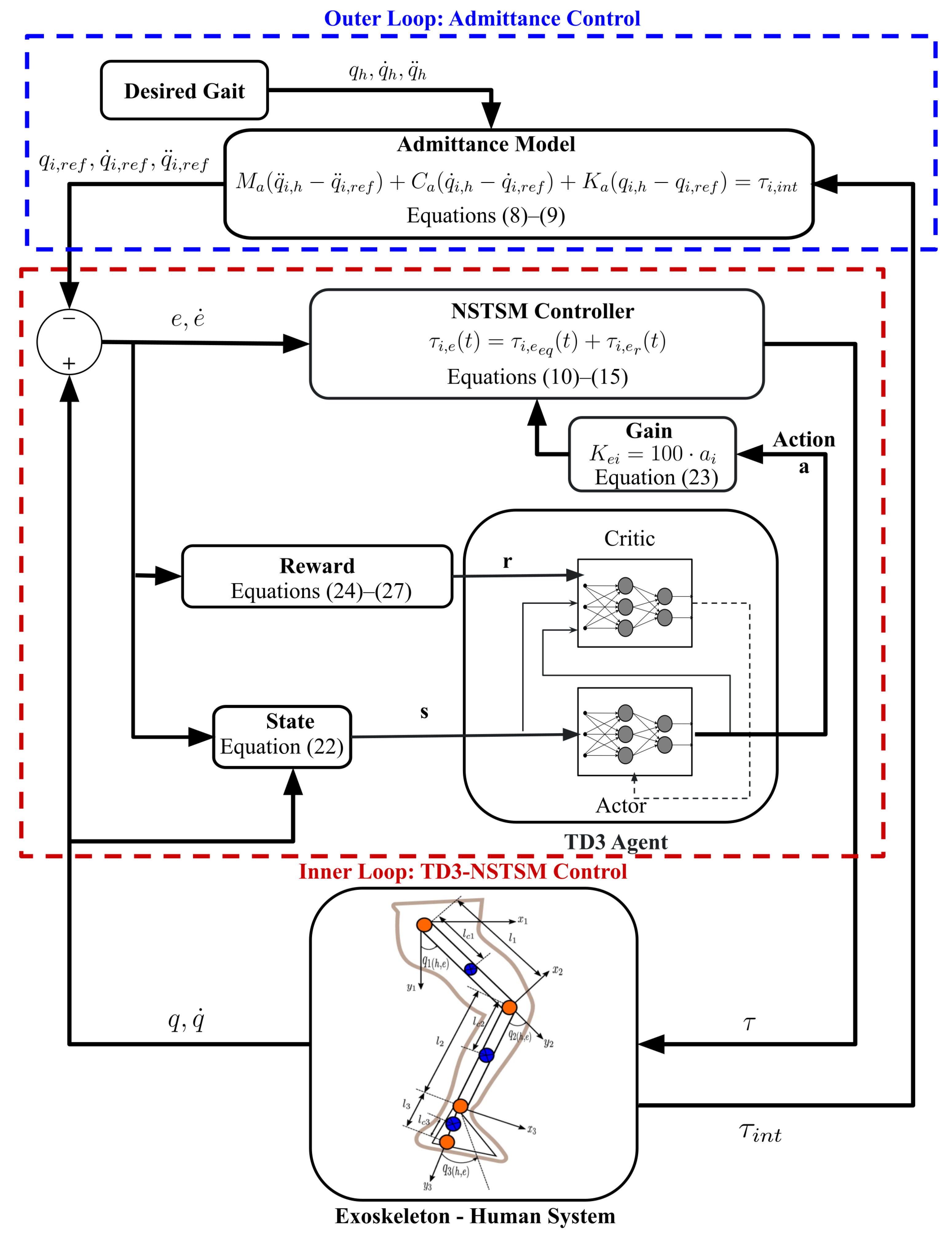
Human-in-the-loop control (see Figure 3) is structured using a layered control approach that encourages active involvement from the user, as outlined earlier in the Introduction. In this study, the outer loop is designed using an admittance control strategy, which interprets interaction forces to adjust motion. Meanwhile, the inner loop implements a robust finite-time sliding-mode method to ensure precise gait tracking. The next subsections detail the development of the admittance controller, followed by the position control strategy tailored for the integrated pediatric exoskeleton system.

3.1. Admittance Control

In the admittance model, the exoskeleton robot can adjust its planned trajectory in reaction to the user’s applied force. Depending on how much the actual exoskeleton path differs from the original gait trajectory, the modified trajectory complies with the interaction force between the subject and the exoskeleton. The coupled subject–exoskeleton system uses a servo-level control scheme to regulate the reference trajectory it adapts. The following version of the admittance model can be applied if the reference trajectory, $q_{i,ref}$, and the intended gait trajectory for a human, $q_{i,h}$, are provided.

$$\begin{array}{cc}\hfill & M_a({\ddot{q}}_{i,h}-{\ddot{q}}_{i,ref})+C_a({\dot{q}}_{i,h}-{\dot{q}}_{i,ref})+K_a(q_{i,h}-q_{i,ref})={\tau }_{i,int}\hfill \end{array}$$

(8)

$$\begin{array}{cc}\hfill & {\ddot{q}}_{i,ref}={\ddot{q}}_{i,h}-M_a^{-1}\left\{C_a({\dot{q}}_{i,h}-{\dot{q}}_{i,ref})+K_a(q_{i,h}-q_{i,ref})-{\tau }_{i,int}\right\}\hfill \end{array}$$

(9)

In this context, $M_a$, $C_a$, and $K_a$ represent the inertial, damping, and stiffness components of the admittance model. In the AA mode explored here, the difference between the desired human motion and the reference trajectory is actively modeled to reflect human–robot interaction.

3.2. NSTSM Trajectory Tracking Control

In traditional terminal sliding-mode (TSM) control, the use of negative fractional powers introduces singularities, which can lead to unbounded control inputs and compromise the system’s performance. To address these issues, this section presents a novel design for a non-singular terminal sliding-mode (NSTSM) controller. The proposed approach offers the advantages of avoiding singularities and demonstrating robustness against parametric uncertainties as well as unmodeled or external disturbances. The discussion begins with a clear definition of the problem, considering the error dynamics, sliding surface, and the newly proposed control law. Following this, a Lyapunov stability analysis is conducted to confirm the finite-time convergence of the system states.

Let ${\zeta }_i=q_{i,e}-q_{i,ref}$ represent the tracking error and ${\dot{\zeta }}_i={ϵ}_i={\dot{q}}_{i,e}-{\dot{q}}_{i,ref}$ denote its derivative. The error dynamics can then be formulated in state-space representation as

$$\left\{\begin{array}{cc}\hfill \dot{{\zeta }_i}& ={ϵ}_{i,e}\hfill \\ \hfill {\dot{ϵ}}_i& =M_{oe}^{-1}\left(q_{i,e}\right)\left(-C_{oe}(q_{i,e},{\dot{q}}_{i,e}){\dot{q}}_{i,e}-{\mathcal{G}}_{oe}\left(q_{i,e}\right)-M_{oe}\left(q_{i,e}\right){\ddot{q}}_{i,ref}-{\tau }_{i,int}+{\tau }_{i,e}+\nu \right)\hfill \end{array}\right.$$

(10)

In the absence of prior knowledge about the upper bounds of dynamic parameters, the following design approach can be utilized for this purpose [39].

$$∥{\mathcal{M}}_{oe}^{-1}\left(q_{i,e}\right)\nu ∥\le \Omega ={\beta }_o+{\beta }_1\parallel q_{i,e}\parallel +{\beta }_2{\parallel {\dot{q}}_{i,e}\parallel }^2$$

(11)

The parameters ${\beta }_0$, ${\beta }_1$, and ${\beta }_2$ are required to be positive, and $q_{i,e}$ along with ${\dot{q}}_{i,e}$ must remain within defined limits to reduce the adverse impact of uncertainties and external disturbances.

Consider the exoskeleton dynamics described in Equation (10), which satisfies the upper bound condition specified in Equation (11) with known constants ${\beta }_0$, ${\beta }_1$, and ${\beta }_2$. If the NSTSM surface $(s_i\forall i=1,2,3)$ is defined as

$$s_i={\zeta }_i+\Lambda {{ϵ}_i}^{a/b}$$

(12)

where $\Lambda =1/\alpha$ is a diagonal design matrix with $\alpha >0$, and a and b are positive odd integers with $a>b$, the proposed control law is expressed as the combination of equivalent control law ${\left({\tau }_{i,e}\right)}_{eq}$ and reaching control law ${\left({\tau }_{i,e}\right)}_r$:

$${\tau }_{i,e}\left(t\right)={{\tau }_{i,e}}_{eq}\left(t\right)+{{\tau }_{i,e}}_r\left(t\right)$$

(13)

where

$$\begin{array}{cc}\hfill {{\tau }_{i,e}}_{eq}\left(t\right)& =-\left(-C_{oe}(q_{i,e},{\dot{q}}_{i,e}){\dot{q}}_{i,e}-G_{oe}\left(q_{i,e}\right)-M_{oe}\left(q_{i,e}\right){\ddot{q}}_{i,ref}-{\tau }_{i,int}+{\displaystyle \frac{b}{a}}{M}_{oe}\left(q_{i,e}\right){\Lambda }^{-1}{{ϵ}_i}^{2-a/b}\right)\hfill \end{array}$$

(14)

and

$${{\tau }_{i,e}}_r\left(t\right)=-{\mathcal{M}}_{oe}\left(q_{i,e}\right)(\Omega +\eta )\mathrm{sat}\left(s_i\right).$$

(15)

Here, the parameters satisfy $1<(a/b)<2$, and $\eta$ is a small positive constant. The use of the $\mathrm{sat}\left(s_i\right)$ function instead of the traditional $\mathrm{sign}\left(s\right)$ function is intended to mitigate chattering effects. Under these conditions, the system’s gait tracking error is guaranteed to converge to zero within a finite time.

Stability Proof

Let us define the proposed Lyapunov function as follows:

$$\mathcal{V}={\displaystyle \frac{1}{2}}{s}_i^T{s}_i$$

(16)

By taking the time derivative of the above function and applying Equation (12), the resulting expression can be obtained.

$$\dot{\mathcal{V}}=s_i^T{\dot{s}}_i=s_i^T\left({ϵ}_i+{\displaystyle \frac{a}{b}}\Lambda {{ϵ}_i}^{(a/b)-1}{\dot{ϵ}}_i\right)$$

(17)

By replacing ${\dot{ϵ}}_i$ as defined in Equation (10) and subsequently applying the relations from Equation (13) through Equation (15),

$$\begin{array}{cc}\hfill \dot{\mathcal{V}}& =s_i^T{\dot{s}}_i\hfill \\ \hfill & =s_i^T\left({ϵ}_i+{\displaystyle \frac{a}{b}}\Lambda {{ϵ}_i}^{(a/b)-1}{M_{oe}}^{-1}\left(q_{i,e}\right)\left(-{\displaystyle \frac{b}{a}}{M}_{oe}\left(q_{i,e}\right){\Lambda }^{-1}{{ϵ}_i}^{2-a/b}+{{\tau }_{i,e}}_r\left(t\right)+\nu \left(t\right)\right)\right)\hfill \\ \hfill & =s_i^T\left({\displaystyle \frac{a}{b}}\Lambda {{ϵ}_i}^{(a/b)-1}{M_{oe}}^{-1}\left(q_{i,e}\right)({{\tau }_{i,e}}_r\left(t\right)+\nu \left(t\right))\right)\hfill \\ \hfill & =s_i^T\left({\displaystyle \frac{a}{b}}\Lambda {{ϵ}_i}^{(a/b)-1}{M_{oe}}^{-1}\left(q_{i,e}\right){{\tau }_{i,e}}_r\left(t\right)\right)+s_i^T\left({\displaystyle \frac{a}{b}}\Lambda {{ϵ}_i}^{(a/b)-1}{M_{oe}}^{-1}\left(q_{i,e}\right)\nu \left(t\right)\right)\hfill \\ \hfill & =-s_i^T\left({\displaystyle \frac{a}{b}}\Lambda {{ϵ}_i}^{(a/b)-1}(\Omega +\eta )sat\left(s_i\right)\right)+s_i^T\left({\displaystyle \frac{a}{b}}\Lambda {{ϵ}_i}^{(a/b)-1}{M_{oe}}^{-1}\left(q_{i,e}\right)\nu \left(t\right)\right)\hfill \\ \hfill & =-s_i^T\left({\displaystyle \frac{a}{b}}\Lambda {{ϵ}_i}^{(a/b)-1}(\Omega +\eta )\left|\right|s_i\left|\right|\right)+s_i^T\left({\displaystyle \frac{a}{b}}\Lambda {{ϵ}_i}^{(a/b)-1}{M_{oe}}^{-1}\left(q_{i,e}\right)\nu \left(t\right)\right)\hfill \end{array}$$

(18)

i.e., using Equation (11),

$$\dot{\mathcal{V}}=-{\eta }_1\left|\right|s_i\left|\right|\le 0,\forall \left|\right|s_i\left|\right|\ne 0$$

(19)

where

$$-{\eta }_1={\displaystyle \frac{a}{b}}\Lambda {{ϵ}_i}^{(a/b)-1}\eta >0$$

According to Lyapunov’s stability criteria, Equation (19) guarantees that the system states asymptotically converge to the origin under the condition that $s_i\left(t\right)=0$. Additionally, to demonstrate the finite-time convergence $\left(t_f\right)$, Equation (19) can be reformulated utilizing Equation (16) as follows:

$$\dot{\mathcal{V}}\le -{\eta }_1\sqrt{2\mathcal{V}}$$

(20)

Reorganizing the inequality and performing integration on both sides

$$\begin{array}{cc}\hfill {\int }_0^{t_f}t& \le -{\displaystyle \frac{{\int }_{\mathcal{V}\left(0\right)}^{\mathcal{V}\left(t_f\right)}{\mathcal{V}}^{-1/2}d\mathcal{V}}{-{\eta }_1\sqrt{2}}}\hfill \\ \hfill \mathrm{or},t_f& \le {\displaystyle \frac{\sqrt{2\mathcal{V}\left(0\right)}}{{\eta }_1}}\hfill \end{array}$$

(21)

Equation (21) demonstrates that the gait tracking error diminishes to zero within a finite time frame, provided the sliding surface $s_i\left(t\right)$ also achieves zero convergence within the same finite duration.

3.3. TD3-Augmented NSTSM

To enhance the robustness and adaptability of the NSTSM controller, we integrate an RL framework based on the TD3 algorithm. In this TD3-NSTSM approach, the RL agent learns to adapt the gains of the diagonal design matrix in Equation (12) in real time based on observed state dynamics and tracking errors. By replacing heuristic gains or fixed tuning rules with a learned policy, the controller continuously adapts to parameter variations, external disturbances, and subject-specific changes, thereby improving tracking accuracy and ensuring more reliable and effective gait rehabilitation assistance.

Remark 2.

The reinforcement learning agent functions solely in inference mode during deployment, with all training conducted offline. NSTSM gains adapted by the TD3 agent remain within pre-defined safe bounds.

3.3.1. RL Environment

The environment is critical to any RL model. Here, the RL environment is designed to simulate the interaction between the lower-limb exoskeleton and its control system. It incorporates the aforementioned dynamics of the human–exoskeleton system and the NSTSM controller as part of the environment. The RL agent interacts with this environment by receiving observations and selecting actions that update control parameters to minimize tracking errors. The key components of the RL environment are described below.

State Space: The state space consists of continuous variables representing the system’s dynamic behavior and tracking performance, including joint angles and velocities to reflect the current state of the exoskeleton joints and position and velocity tracking errors that indicate deviations from the reference trajectory. Consequently, the state vector for each joint is five-dimensional and is defined as

$$s_t={\left[\begin{array}{c}{q}_{i,ref},q_{i,e},{\dot{q}}_{i,e},{\zeta }_i,{\dot{\zeta }}_i\end{array}\right]}^T$$

(22)

where $q_{i,ref}$ is the reference position, $q_{i,e}$ and ${\dot{q}}_{i,e}$ are current joint positions and velocities, and ${\zeta }_i$ and ${\dot{\zeta }}_i$ are current position and velocity errors, as mentioned earlier.

Since there are three joints, the combined state vector has 15 dimensions. Each dimension is bounded to a realistic range of values based on the limits of the exoskeleton and the baseline performance of the NSTSM controller.

Action Space: The action space is a continuous 3-dimensional vector a $=[a_1,a_2,a_3]$, corresponding to the hip, knee, and ankle joints. Each action component is used to adaptively tune the diagonal design matrix $\Lambda =\mathrm{diag}(K_{e1},K_{e2},K_{e3})$ of the NSTSM controller (see Equation (12)). Specifically, the mapping is defined as

$$K_{ei}=100·a_i,a_i\in [0.01,1],i\in \{1,2,3\}$$

(23)

This results in effective gain values $K_{ei}\in [1,100]$, allowing the RL agent to modulate the convergence behavior of each joint’s sliding surface independently. This formulation ($K_{ei}>1$) ensures all actions remain within a physically meaningful and safe range for pediatric exoskeleton actuation. By varying these gains online, the controller can adapt to changing dynamics and user-specific characteristics without requiring manual gain tuning or precise system modeling. To further ensure safe and realistic control, actuator saturation limits were enforced during simulation. Torque outputs were clipped at 50 Nm for the hip, 20 Nm for the knee, and 5 Nm for the ankle, consistent with the rated capabilities of the LLES v2 exoskeleton actuators.

Reward Function: The reward function is designed to guide the RL agent toward achieving precise gait trajectory tracking. The reward starts with a default value of 1 and is reduced based on the deviation from the reference trajectory. At each time step t, the reward $R_t$ is defined as

$$R_t=1-w_{pos}{r}_{pos}-w_{vel}{r}_{vel}$$

(24)

where $w_{pos}$ and $w_{vel}$ are the weights of the combined position error reward $r_{pos}$ and combined velocity error reward $r_{vel}$, respectively.

The combined position error reward $r_{pos}$ is given by

$$r_{pos}=w_{ph}·r_{ph}+w_{pk}·r_{pk}+w_{pa}·r_{pa},$$

(25)

where $w_{ph}$, $w_{pk}$, and $w_{pa}$ are the weights for the position errors of the hip ($r_{ph}$), knee ($r_{pk}$), and ankle ($r_{pa}$) joints, respectively.

Similarly, the combined velocity error reward $r_{vel}$ is given by

$$r_{vel}=w_{vh}·r_{vh}+w_{vk}·r_{vk}+w_{va}·r_{va},$$

(26)

where $w_{vh}$, $w_{vk}$, and $w_{va}$ are the weights for the velocity errors of the hip ($r_{vh}$), knee ($r_{vk}$), and ankle ($r_{va}$) joints, respectively.

The position/velocity error reward for each joint j is calculated as

$$r_i={\displaystyle \frac{\min \left(\left|{\zeta }_i\right|,{\max }_i\right)}{{\max }_i}},$$

(27)

where ${\zeta }_i$ represents the position/velocity error for joint i, and ${\max }_i$ is the maximum allowable error for that joint. This maximum is determined based on the expected errors regarding the baseline NSTSM performance, as well as the limits of the exoskeleton.

The weights in each equation are selected to uniformly sum to one. Consequently, the overall reward $R_t$ is bounded $[0,1]$ to help prevent numerical instability during training. This is particularly relevant for policy gradient algorithms where large reward values can lead to exploding gradients or overly aggressive updates.

3.3.2. Twin Delayed Deep Deterministic Policy Gradient (TD3)

TD3 is an actor–critic RL algorithm designed for continuous control tasks—such as exoskeleton control. It builds upon the deep deterministic policy gradient (DDPG) algorithm by addressing overestimation bias in value function approximation and improving stability during training [40]. TD3 achieves these improvements through three key modifications: clipped double-Q learning, target policy smoothing, and delayed policy updates.

In TD3, the state of the system at time t is represented as $s_t\in {\mathbb{R}}^n$ and the action as $a_t\in {\mathbb{R}}^m$. The algorithm maintains two critic networks, $Q_{{\theta }_1}(s,a)$ and $Q_{{\theta }_2}(s,a)$, parameterized by ${\theta }_1$ and ${\theta }_2$, which approximate the state–action value function. The actor network, ${\pi }_{\varphi }\left(s\right)$, parameterized by $\varphi$, maps the state to a deterministic action. A replay buffer $\mathcal{D}$ stores transitions $(s_t,a_t,r_t,s_{t+1})$, enabling the algorithm to sample data uniformly for updates.

Clipped Double-Q Learning

To mitigate overestimation bias, TD3 uses two independent critic networks and takes the minimum of their value estimates when computing the target value [40]:

$$y_t=r_t+\gamma \underset{i=1,2}{\min }{Q}_{{\theta }_i}^{\mathrm{target}}(s_{t+1},{\tilde{a}}_{t+1}),$$

(28)

where $\gamma$ is the discount factor, and $Q_{{\theta }_i}^{\mathrm{target}}$ is the slowly updated target version of the i-th critic network. The target action ${\tilde{a}}_{t+1}$ is computed as

$${\tilde{a}}_{t+1}={\pi }_{\varphi }^{\mathrm{target}}\left(s_{t+1}\right)+ϵ,$$

(29)

where ${\pi }_{\varphi }^{\mathrm{target}}$ is the target actor network, and $ϵ\sim \mathrm{clip}\left(\mathcal{N}\right(0,\sigma ),-c,c)$ is clipped Gaussian noise added to smooth the policy and improve robustness. The loss for each critic is given by

$$L_{{\theta }_i}={\mathbb{E}}_{(s_t,a_t,r_t,s_{t+1})\sim \mathcal{D}}\left[{(y_t-Q_{{\theta }_i}(s_t,a_t))}^2\right],i=1,2.$$

(30)

Delayed Policy Updates

TD3 updates the actor network less frequently than the critic networks to improve training stability. Specifically, after every d updates to the critics, the actor is updated using the deterministic policy gradient [40]:

$${\nabla }_{\varphi }J\left(\varphi \right)={\mathbb{E}}_{s_t\sim \mathcal{D}}\left[{\nabla }_a{Q}_{{\theta }_1}{(s,a)|}_{a={\pi }_{\varphi }\left(s\right)}{\nabla }_{\varphi }{\pi }_{\varphi }\left(s\right)\right].$$

(31)

The target networks for both actor and critics are updated using a soft update rule:

$${\varphi }^{\mathrm{target}}\leftarrow \rho \varphi +(1-\rho ){\varphi }^{\mathrm{target}},{\theta }_i^{\mathrm{target}}\leftarrow \rho {\theta }_i+(1-\rho ){\theta }_i^{\mathrm{target}},$$

(32)

where $\rho \in (0,1)$ is the update rate (target smooth factor). Note that the symbol $\rho$ is used here instead of the standard notation $\tau$ since $\tau$ represents torque in this work.

Target Policy Smoothing

To prevent overfitting and reduce variance in the target value estimate, noise $ϵ$ is added to the target action during critic updates. The noise is clipped to a small range $[-c,c]$ to ensure that the target remains near the learned policy [40]:

$$ϵ\sim \mathrm{clip}\left(\mathcal{N}\right(0,\sigma ),-c,c).$$

(33)

This modification ensures that the learned policy is robust to small perturbations and avoids exploiting narrow peaks in the value function.

These enhancements make TD3 more robust and stable than the predecessor in DDPG for continuous control problems, addressing issues like overestimation bias and instability while maintaining efficient learning in high-dimensional action spaces.

3.3.3. Hyperparameter Tuning

The selection and tuning of hyperparameters play a crucial role in the training performance and stability of RL agents such as TD3. Key hyperparameters include the learning rates of the actor and critic networks (${\alpha }_{\mathrm{act}}$ and ${\alpha }_{\mathrm{cr}}$), the target smooth factor ($\rho$), the discount factor ($\gamma$), and the exploration noise parameters ($\sigma$), all of which can significantly influence the agent’s learning behavior.

The learning rates control how quickly the networks update their weights in response to gradient signals. Lower learning rates promote stable convergence but can result in slower learning, while higher rates accelerate learning at the risk of instability or suboptimal convergence. Proper selection ensures that the networks adapt efficiently to the exoskeleton control task without diverging or overfitting. The discount factor ($\gamma$) determines the relative importance of future rewards compared to immediate rewards. A higher discount factor ($\gamma \to 1$) encourages the agent to prioritize long-term performance, which can improve overall policy robustness but may introduce additional computational complexity. Conversely, a lower discount factor biases the agent toward short-term rewards, which can enhance responsiveness to real-time disturbances—a critical feature for practical exoskeleton control applications. Exploration noise parameters, particularly Gaussian noise in TD3, regulate the agent’s exploration of the action space during training. Appropriately tuned noise parameters ensure a balance between exploration and exploitation. Excessive exploration can delay convergence, while insufficient exploration may result in the agent becoming trapped in suboptimal policies. To address this, our training process employs an exploration schedule, where exploration is emphasized in early episodes and gradually reduced in later stages to encourage exploitation of the learned policy. Additional factors, such as batch size and the target network update frequency, also impact the training process. A larger batch size tends to stabilize policy updates by reducing variance, although at the expense of increased computational requirements. The target smooth factor ($\rho$) governs the rate of updates to the target networks; smaller values ensure gradual changes, which contribute to more stable learning.

3.4. Implementation and Training

The proposed human-in-the-loop control framework, with the novel TD3-NSTSM, is implemented using Simulink combined with MATLAB 2024b’s reinforcement learning Toolbox. This platform provides an intuitive interface for creating custom environments and for training and evaluating reinforcement learning agents. The control parameters used in the baseline NSTSM controller are summarized in

Table 3. Control parameters used in the NSTSM controller.

Parameter	Value
a	13
b	9
$\eta$	2
${\beta }_0$	24
${\beta }_1$	14
${\beta }_2$	6
$K_{e1}$	100
$K_{e2}$	100
$K_{e3}$	100

. For the TD3 agent, optimized for the exoskeleton control task, the training and model configurations are summarized in

Table 4. Key hyperparameters for training the TD3 agent.

Parameter	Value
General Training Options
Max steps per episode	2000
Discount factor ($\gamma$)	0.99
Target Smooth Factor ($\rho$)	0.005
Mini-batch size	256
Experience buffer length	5 × 104
Sample time	0.001
Target Policy Smoothing Parameters
Mean	0
Standard deviation	0.447
Standard deviation decay rate	0
Minimum standard deviation	0.1
Lower limit	−0.5
Upper limit	0.5
Exploration Noise Parameters
Standard deviation (${\sigma }_n$)	0.7
Standard deviation decay rate	1 × 10−5
Minimum standard deviation	0.1
Lower limit	−Inf
Upper limit	Inf
Actor and Critic Networks
Learning rate—actor (${\alpha }_{\mathrm{act}}$)	0.01
Learning rate—critic 1 (${\alpha }_{\mathrm{cr}1}$)	0.01
Learning rate—critic 2 (${\alpha }_{\mathrm{cr}2}$)	0.003
Gradient threshold	inf
Gradient threshold method	L2norm
L2 regularization factor	1 × 10−4
Optimizer	adam
Optimizer parameters (epsilon)	1 × 10−8
Optimizer parameters (gradient decay factor)	0.9
Optimizer parameters (squared gradient decay factor)	0.999
Device used	gpu

. To fine-tune these hyperparameters, Bayesian optimization was employed, with the objective of maximizing episodic return. This method systematically explores the hyperparameter space, allowing for the identification of optimal settings.

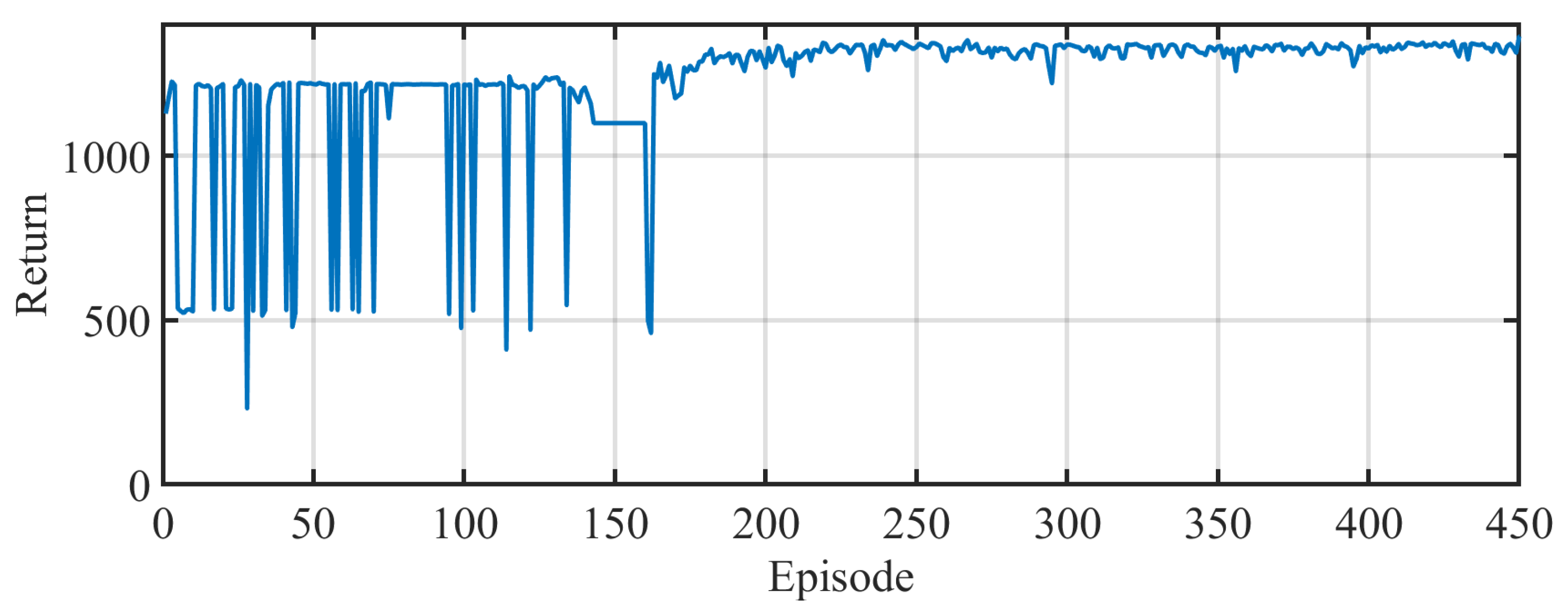
The training performance of the TD3 agent is illustrated in Figure 4, which shows the learning curve over 450 episodes. The early phase (approx. episodes 0–200) is characterized by high variability in return, indicative of the agent’s exploratory behavior as it searched the action space to learn effective gain combinations. After this exploratory phase, the best-performing model was saved based on return and thus controller performance. In the subsequent phase (episodes 200–450), the agent was fine-tuned from this checkpoint, leading to a marked increase in return stability and convergence to a robust policy. This two-stage training strategy enabled efficient policy refinement and accelerated convergence toward optimal gain tuning.

3.5. Model Evaluation

The performance of the TD3-NSTSM controller within the wider human-in-the-loop control scheme is evaluated through numerical simulations conducted in MATLAB. The evaluation focuses on the controller’s tracking performance based on the following metrics:

• Maximum Absolute Deviation (MAD): Quantifies the maximum tracking error observed across the gait cycle.
• Root Mean Square Error (RMSE): Measures the overall accuracy of the exoskeleton in tracking the desired gait trajectory.

  $$\mathrm{RMSE}=\sqrt{{\displaystyle \frac{1}{T}}\sum _{t=1}^T{{\zeta }_t}^2}.$$

  (34)
• Integral of Absolute Error (IAE): Evaluates the total accumulated error over time.

  $$\mathrm{IAE}={\int }_0^T\left|\zeta \left(t\right)\right|dt,$$

  (35)

  where T is the total duration of the evaluation and $\zeta \left(t\right)$ is the tracking error as a function of time.

4. Results

This section presents and compares the results for the proposed human-in-the-loop control framework with an inner-loop TD3-NSTSM controller against the same framework with a standalone NSTSM controller, highlighting the performance and adaptability of the RL framework. The uncertainty parameter and disturbance vector are defined as $\delta =0.1$ and ${\tau }_D={[5\sin \left(2\pi t\right),3\sin \left(\pi t\right),\sin \left(\pi t\right)]}^T$, respectively. The analysis begins with a comparison of joint-space trajectory tracking performance, quantified by the RMSE, MAD, and IAE metrics. This is followed by an evaluation of Cartesian tracking accuracy. A torque analysis is then provided to assess the efficiency of the different control strategies. Finally, a gain analysis illustrates how the TD3 agent adapts the inner-loop NSTSM control parameters throughout the gait cycle.

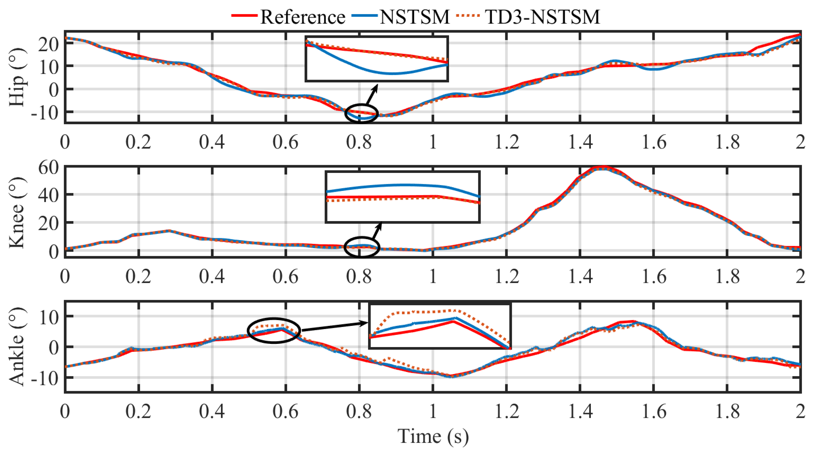
4.1. Tracking Performance: Joint Space

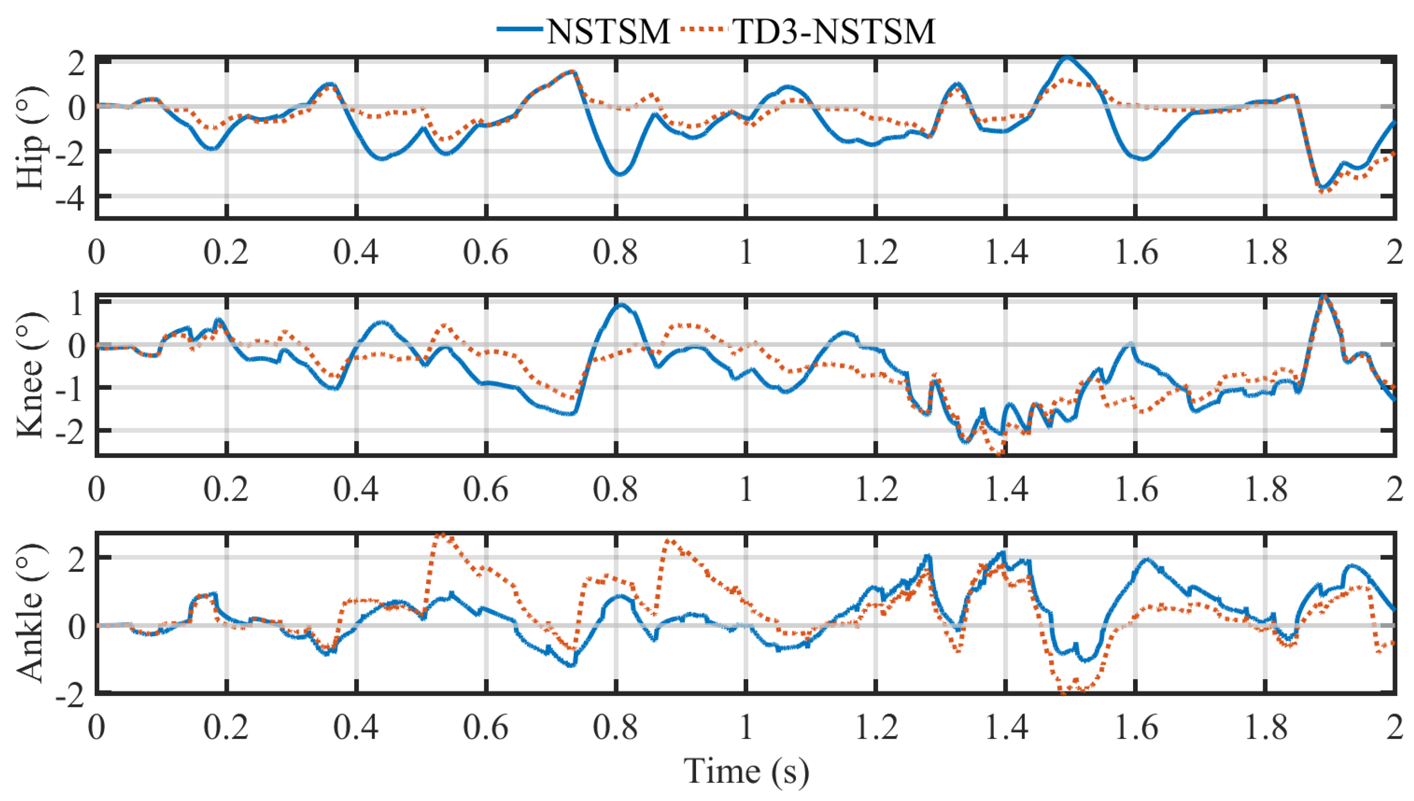
Figure 5 and Figure 6 illustrate the joint-space tracking performance of the baseline NSTSM and the proposed TD3-NSTSM for the hip, knee, and ankle joints. Figure 5 compares the reference trajectory (solid red) with the trajectories achieved by each controller, highlighting key regions where differences are most pronounced. Figure 6 presents the corresponding tracking errors over time, showing how each controller responds throughout the gait cycle.

Table 5. Summary of computed metrics for each joint and improvements attained by TD3-NSTSM.

Metric	Joint	NSTSM	TD3-NSTSM	Improvement (%)
MAD (°)	Hip	3.61	3.83	−6.09
	Knee	2.30	2.60	−13.04
	Ankle	2.2	2.74	−24.55
RMSE (°)	Hip	1.33	0.96	27.82
	Knee	0.92	0.87	5.43
	Ankle	0.81	0.97	−19.75
IAE (°·s)	Hip	2.13	1.26	40.85
	Knee	1.47	1.32	10.20
	Ankle	1.27	1.44	−13.39

complements the visual analysis by providing a quantitative summary of the maximum absolute deviation (MAD), root mean square error (RMSE), and integrated absolute error (IAE) for each joint, along with the percentage improvements achieved by TD3-NSTSM.

For the hip joint, TD3-NSTSM demonstrates clear improvement over the baseline NSTSM controller. The observed trajectory tracks the reference more closely, especially during transitions, as emphasized by the inset in Figure 5. The error curve in Figure 6 shows consistently lower deviations for TD3-NSTSM across most of the gait cycle. Quantitatively, TD3-NSTSM reduces the RMSE by 27.82% and IAE by 40.85%, although the MAD slightly increases by 6.09%, possibly due to brief overshoots in specific segments. For the knee joint, TD3-NSTSM also improves tracking accuracy across all the metrics. Figure 5 shows better alignment with the reference trajectory, particularly during the mid-swing phase, while the error plot in Figure 6 reveals reduced peak errors. TD3-NSTSM achieves a 5.43% reduction in RMSE and a 10.20% reduction in IAE, although the MAD again shows a modest increase of 13.04%, suggesting more frequent—but smaller—corrections over time. For the ankle joint, TD3-NSTSM does not show consistent improvements over the baseline. As seen in Figure 5, both controllers follow the reference trajectory reasonably well, but TD3-NSTSM exhibits greater deviations during certain portions of the gait cycle. The error plot in Figure 6 highlights larger fluctuations in the TD3-NSTSM error profile, particularly in the early and mid-stance phases. This is reflected quantitatively by increases in all three error metrics: MAD rises by 24.55%, RMSE by 19.75%, and IAE by 13.39%. These degradations may stem from the more complex dynamics and higher sensitivity of the ankle joint to rapid trajectory changes. Overall, the results demonstrate that TD3-NSTSM effectively enhances the tracking performance for the hip and knee joints, with moderate trade-offs at the ankle.

Furthermore, when comparing the performance of the TD3-NSTSM controller with other state-of-the-art approaches such as fuzzy adaptive sliding-mode control (FASMC) [41], it appears that NSTSM shows considerably reduced MAD at both the hip (3.83° vs. 3.96°) and knee joints (2.60° vs. 2.94°). However, such a comparison is not fully justified as the FASMC [41] was designed for an entirely different lower-limb exoskeleton design with varying system dynamics, uncertainties, and external perturbations. Moreover, the authors in [41] did not account for human–exoskeleton interaction effects, which are explicitly addressed in our work.

4.2. Tracking Performance: Cartesian Space

Figure 7 presents the foot trajectory tracking performance in the Cartesian plane, comparing the reference trajectory with those generated by NSTSM and TD3-NSTSM. While both controllers approximate the target loop, TD3-NSTSM follows the trajectory more closely, especially during the terminal swing phase.

The inset highlights a region near the end of the gait cycle where TD3-NSTSM significantly reduces deviation compared to NSTSM, which exhibits more noticeable overshooting and undershooting. This improvement suggests that adaptive gain tuning enables more precise path following in two-dimensional space—crucial for maintaining smooth and symmetric gait patterns during gait rehabilitation.

4.3. Torque Analysis

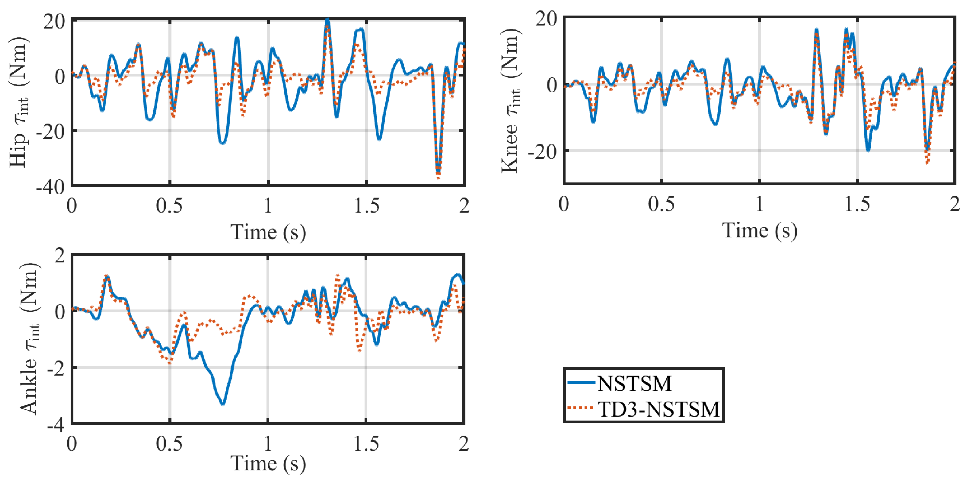
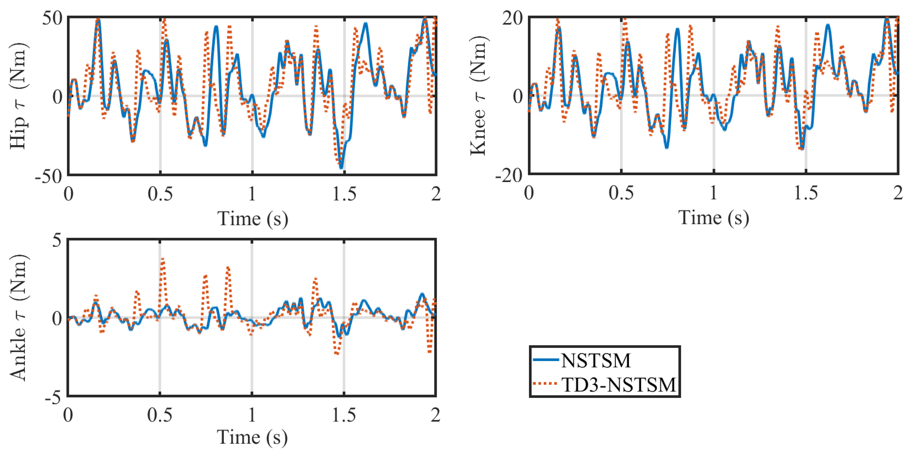
Figure 8 and Figure 9 present the interaction torques and applied control torques for the hip, knee, and ankle joints under both NSTSM and TD3-NSTSM. Figure 8 shows the measured interaction torques between the user and the exoskeleton, revealing significant joint-dependent variability across the gait cycle. At the hip joint, TD3-NSTSM generally reduces interaction torques compared to NSTSM, with typical reductions of about 5–15 Nm. However, near the end of the gait cycle, there is a notable peak where both controllers exhibit similar magnitudes. The knee joint shows reduced interaction torques under TD3-NSTSM for much of the gait cycle; however, after about t = 1.25 s, the reduction becomes less consistent, with TD3-NSTSM at times producing higher interaction torques than NSTSM. For the ankle joint, TD3-NSTSM effectively reduces interaction torques during the first half of the gait cycle, particularly by mitigating a major spike; however, it shows less consistent behavior in the second half. These patterns suggest that TD3-NSTSM offers more compliant and comfortable assistance by better accommodating user movements and reducing user–exoskeleton conflict, although further refinement is needed to ensure consistent performance across all the gait phases.

Figure 9 compares the actuator torques generated by each controller. To improve visual clarity and emphasize the overall trends in Figure 9, a moving average and a Savitzky–Golay filter were applied to smooth both NSTSM and TD3-NSTSM signals. Overall, both controllers produced periodic torque patterns, with TD3-NSTSM generally exhibiting sharper peaks and corrections. This behavior reflects the controllers’ adaptive gain adjustments, which respond more aggressively to tracking errors—particularly evident in the hip and knee joints. In contrast, at the ankle joint, the torque magnitude is lower and more stable for both controllers, although TD3-NSTSM displays slightly more high-frequency variability.

Table 6. Chattering index comparison between NSTSM and TD3-NSTSM.

Joint	NSTSM CI	TD3-NSTSM CI	% Change
Hip	51.86	50.57	$-2.49$%
Knee	21.87	21.18	$-3.14$%
Ankle	2.71	2.70	$-0.11$%

quantifies the chattering behavior using the chattering index (CI) [42]. Although chattering is characteristic of sliding-mode control, the NSTSM control avoids chattering by using a saturation function instead of the signum function, as mentioned in Section 3.2. Moreover, in our proposed RL-NSTSM implementation, the reinforcement learning component helped to mitigate chattering by achieving a reduction of 2.49% at the hip and 3.1% at the knee through responsive tuning of the NSTSM gains. It is also pertinent to mention that the CI observed with NSTSM and TD3-NSTSM is significantly less compared to conventional sliding-mode control schemes, with a range of ${10}^3$–${10}^4$ [42].

Overall, these results suggest that TD3-NSTSM not only delivers more assertive yet targeted control at high-load joints but also provides assistance that could enhance user comfort and engagement by minimizing unnecessary user–exoskeleton conflict.

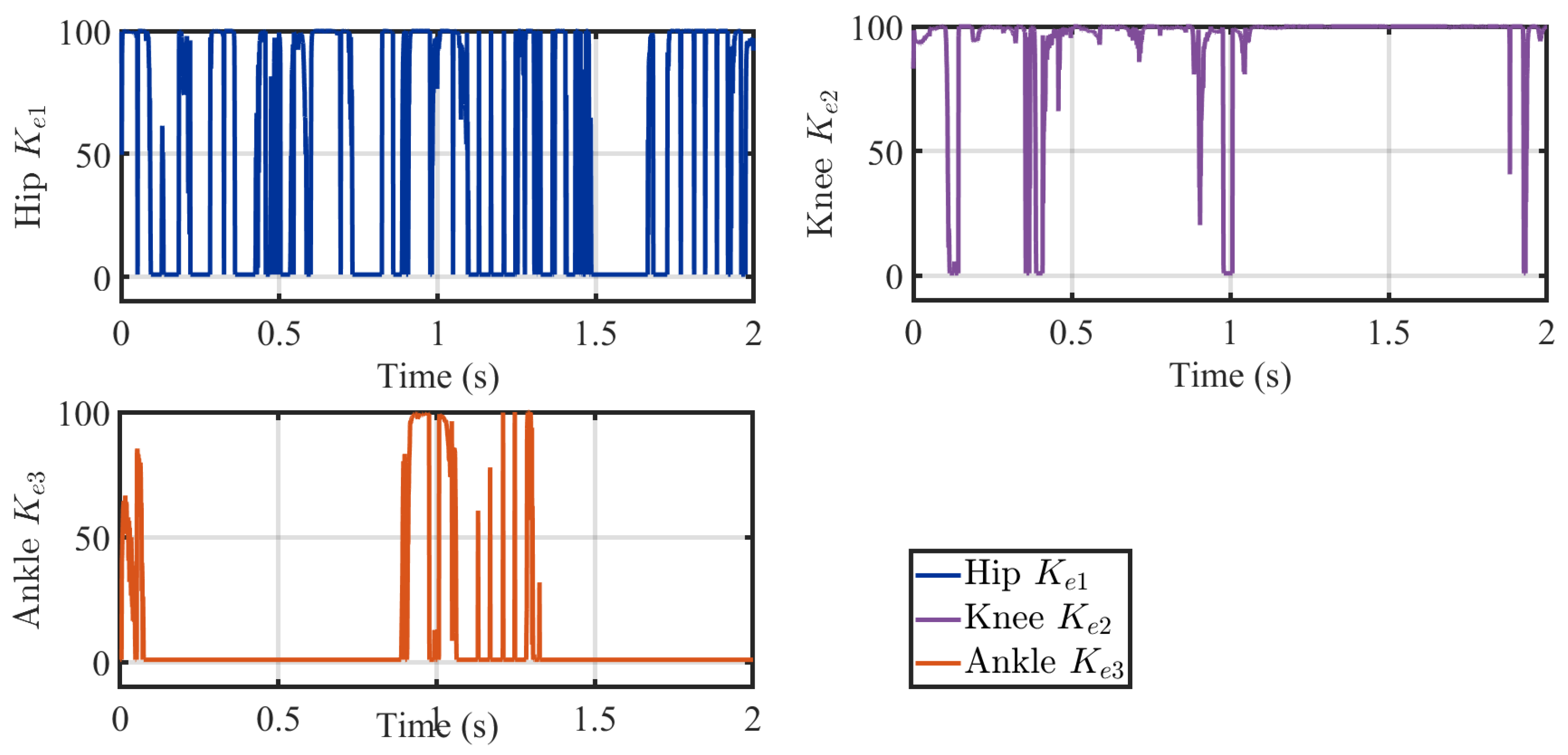
4.4. Gain Analysis

Figure 10 shows the time-varying gain values $K_{e1}$, $K_{e2}$, and $K_{e3}$ for the hip, knee, and ankle joints, respectively, as adapted by the TD3 agent during the gait cycle. The results highlight how the reinforcement learning policy modulates these gains in response to joint-specific dynamics and tracking demands. At the hip, $K_{e1}$ fluctuates frequently to provide rapid corrections during phases of high load transfer. The knee gain $K_{e2}$ exhibits periods of near-maximal values, suggesting stronger corrective effort during stance transitions, while the ankle gain $K_{e3}$ shows more sporadic activation, reflecting both the lower torque requirements and the agent’s less consistent tuning at this joint. These patterns demonstrate how TD3-NSTSM adaptively allocates control authority across joints, although the variability at the ankle indicates further refinement may be needed to achieve smoother gain modulation.

5. Discussion

The results of this study demonstrate that the proposed human-in-the-loop controller, comprising outer-loop admittance control and an inner-loop TD3-NSTSM controller, improves the gait tracking of a pediatric exoskeleton in AA mode. By integrating reinforcement learning with a model-based NSTSM control scheme, the hybrid controller achieved reduced tracking errors in both joint and Cartesian spaces, along with sharper and more responsive torque profiles in high-load joints such as the hip and knee. These findings suggest that real-time adaptation of control gains via deep reinforcement learning can compensate for modeling uncertainties and joint-specific dynamics in pediatric gait rehabilitation. TD3-NSTSM also reduced peak interaction torques compared to the baseline NSTSM controller, indicating more compliant assistance that may enhance user comfort, engagement, and motor learning.

This work advances the field in two primary directions: (i) improving robustness through model-based frameworks and (ii) enabling online adaptability using deep reinforcement learning. Traditional inner-loop controllers such as SMC and NSTSM control have shown strong robustness to disturbances and parameter variations [18,43] but rely on fixed gains or heuristic offline tuning, limiting their responsiveness to dynamic user-specific changes during gait. Recent efforts to introduce learning-based adaptivity have shown promise. Hfaiedh et al. [22] used DDPG to tune gains in an NSTSM controller for upper-limb rehabilitation, while Luo et al. [21] employed PPO to adjust assistance levels in lower-limb gait tasks. Sun et al. [27] used a TD3-based residual reinforcement learning framework to fine-tune PID control for soft exosuits, achieving significant improvements in metabolic efficiency during real-world trials. Li et al. [28] combined TD3 with an active disturbance-rejection controller (ADRC) for lower-limb exoskeletons, demonstrating enhanced tracking and robustness to disturbances in both simulation and experimental settings.

While Sun et al. [27] applied TD3 to fine-tune PID gains, our method directly modulates the gains of an NSTSM controller—a more robust nonlinear framework with finite-time convergence and improved resilience to disturbances. The observed improvements in hip and knee tracking validate this deeper integration of learning with robust control. However, the ankle joint remains a challenge, likely due to its lower torque requirements, increased sensitivity to trajectory timing, or convergence to a suboptimal policy. These characteristics may necessitate joint-specific learning strategies or adaptive reward weighting to achieve more consistent performance.

Despite its advantages, the TD3-NSTSM controller has certain limitations. Although the simulation includes interaction torques to emulate user input and operates in AA mode, it remains an idealized environment that omits real-world complexities such as sensor noise, joint friction, and inference latency. Additionally, because the TD3 policy is deployed in inference mode without online learning, its effectiveness depends heavily on the quality and diversity of the offline training data. Furthermore, the inner loop NSTSM control can be improved by exploiting the latest disturbance-rejection controllers [28,44,45]. On the other hand, exposure to a broader range of patient variability, including variations in effort, fatigue, engagement, and pathological gait patterns such as spasticity, is needed to improve generalization. Finally, while user effort is partially modeled, direct sensing of human intent (e.g., via EMG or force sensors) was not incorporated. These limitations must be addressed through hardware implementation and user-in-the-loop testing prior to clinical deployment.

6. Conclusions

This work introduced a human-in-the-loop control framework combining outer-loop admittance control with a novel TD3-NSTSM inner-loop controller for pediatric lower-limb exoskeletons. The system dynamically adapts both the reference trajectory and control gains in response to user interaction forces and gait tracking demands. The simulation results show that TD3-NSTSM reduced the RMSE at the hip and knee by 27.82% and 5.43%, respectively, and the IAE by 40.85% and 10.20%, while generating responsive control torques that better accommodate joint-specific dynamics. Although the ankle tracking performance was less consistent, the approach maintained stable adaptive control throughout the gait cycle, highlighting areas for further refinement. The reduction in peak interaction torques further indicates the potential of TD3-NSTSM to provide more comfortable and user-aligned assistance.

Future work should focus on real-time implementation of this layered control architecture on the LLES v2 exoskeleton, including robust safety mechanisms, to validate its robustness under unstructured conditions. Enhancing the outer loop with biosignal-based intent detection (e.g., EMG or force sensors) could further personalize assistance in line with assist-as-needed principles. To address the current limitations, researchers should conduct ablation studies to evaluate reward sensitivity and explore joint-specific learning strategies. Furthermore, improving the diversity of the offline dataset through variation in gait profiles, user dynamics, and simulated disturbances will help to ensure that the learned policy generalizes across a wide range of patient scenarios. Ultimately, clinical trials will be necessary to assess the therapeutic impact, usability, and long-term efficacy, ensuring that the proposed human-in-the-loop controller translates effectively into pediatric gait rehabilitation practice.