


End-of-Line Quality Control Based on Mel-Frequency Spectrogram Analysis and Deep Learning


Abstract
1. Introduction
- A deep learning-based classification model using a CNN–BiGRU architecture trained on MFSs generated from acoustic and vibration signals of BLDC motors.
- An evaluation strategy that includes bootstrap resampling to estimate 95% confidence intervals, providing a more robust estimate of model reliability.
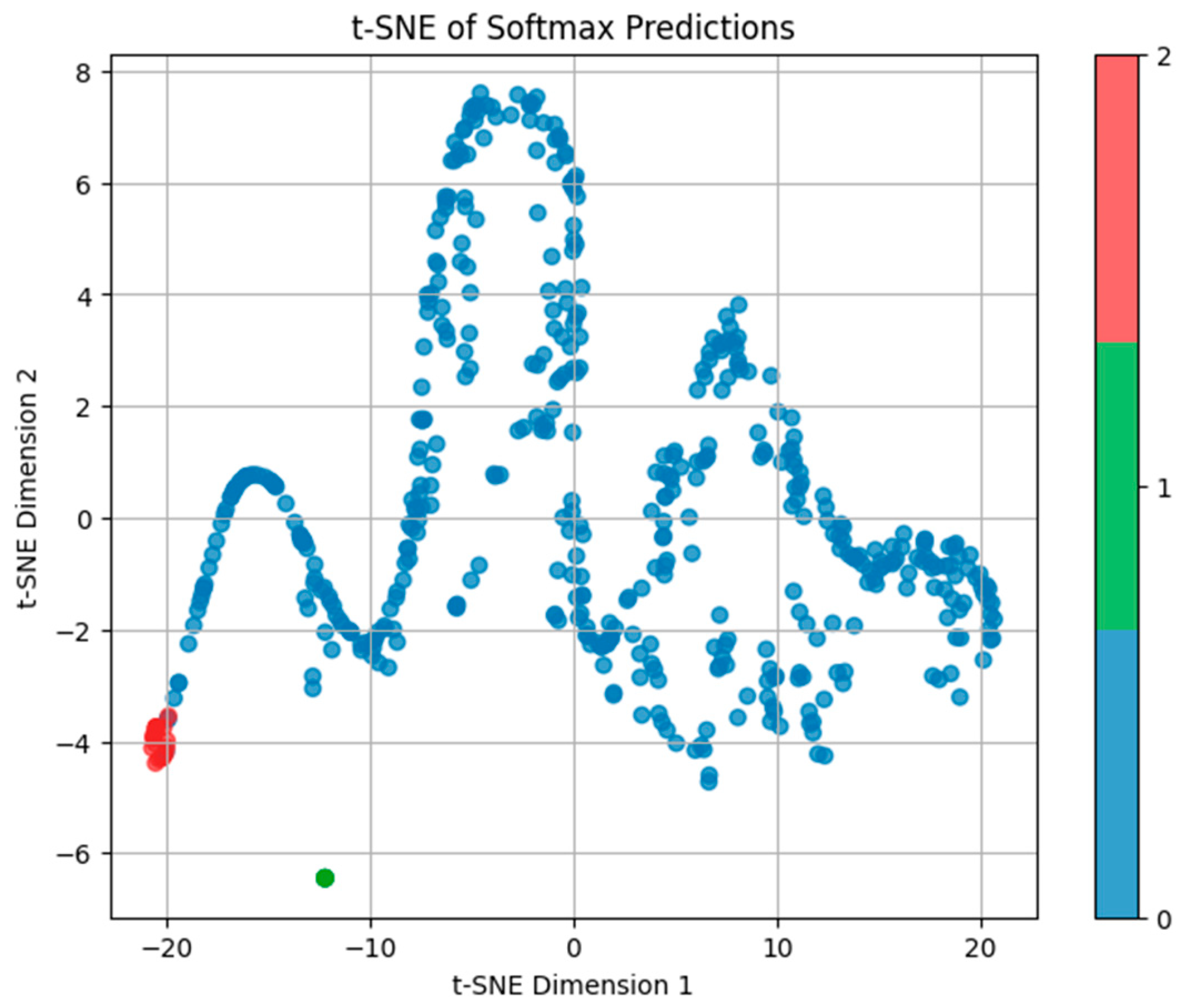
- The use of t-SNE visualization to analyse feature resolution and improve the interpretability of the learned representations in the output space.
- Section 2 describes the problem and outlines key challenges.
- Section 3 presents the proposed fault detection approach.
- Section 4 explains the data preparation and feature reduction process.
- Section 5 describes the neural network architecture and training procedure.
- Section 6 presents classification results and performance evaluation.
- Section 7 concludes the paper and discusses future directions.
2. Problem Description
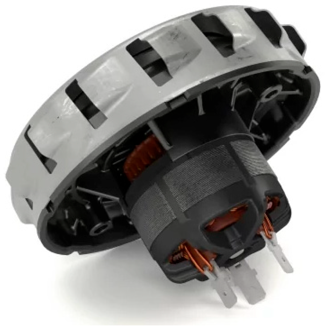
2.1. Motor Description
2.2. Existing EoL Quality Algorithm and Inspection System
3. Proposed Novel EoL Quality Inspection Algorithm
3.1. Overview
- MFSs are used to transform raw time-series signals into 3D time–frequency representations that can be presented as a colour image;
- A hybrid deep learning architecture that combines a CNN and a BiGRU network.
3.2. MFSs
- Efficient dimensionality reduction while preserving perceptually and diagnostically relevant features;
- Enhanced sensitivity in the low- and mid-frequency ranges (up to 5 kHz), where mechanical issues such as imbalance, misalignment, and bearing defects usually occur;
- Increased robustness to noise and minor variations in signal phase or speed.
3.3. Neural Network Architecture: CNN–BiGRU
4. Data Preparation
4.1. Data Structure
- Class 0: motors with no detected faults (good);
- Class 1: motors with faults detected in TC 2;
- Class 2: motors with faults detected in TC 3.
4.2. MFS Generation
4.3. MFS Processing and Dimensionality Reduction
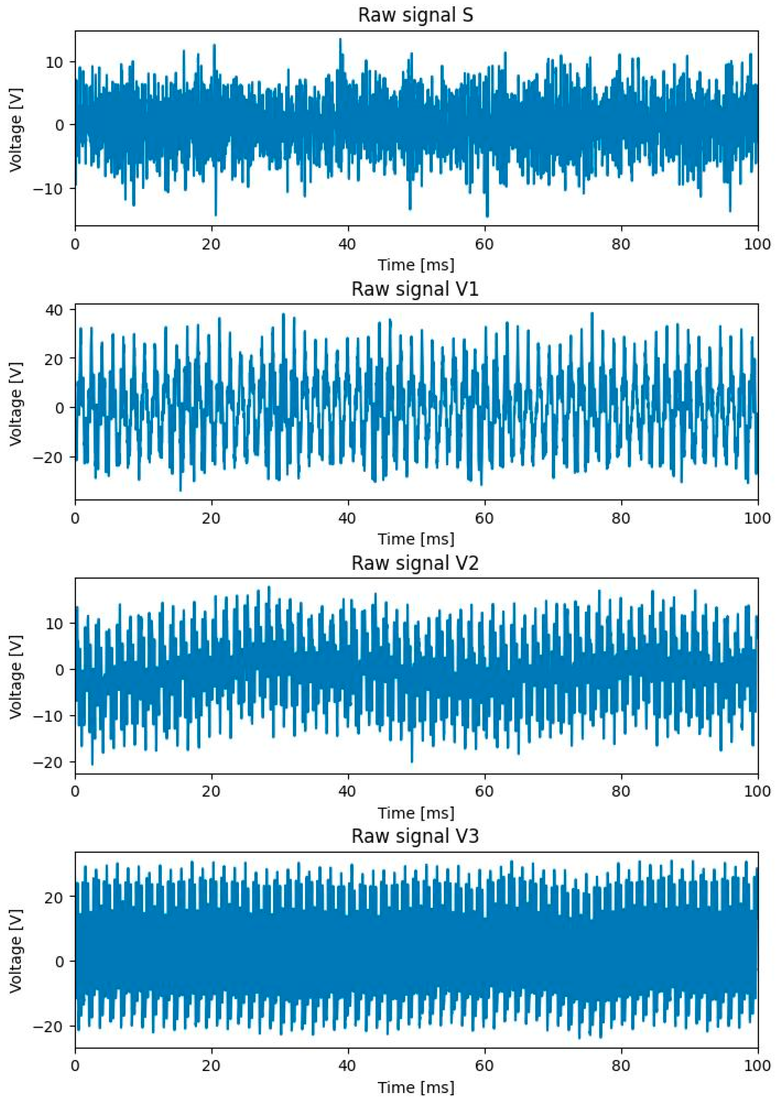
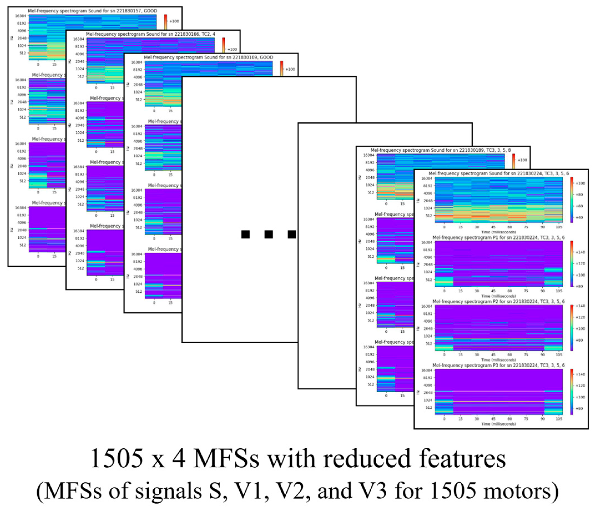
- Step 1: MFS creation. In this step, raw time–domain signals of each motor (V1, V2, V3, and S, explained in Section 4.1) are converted into 4 MFSs, according to parameter settings from 0. The results of this step are 4 MFSs of size 2048 (frequency bands) × 7 (time frames) for each motor. The measured latency for generating all 4 MFSs for one motor is approximately 0.1231 s, which is acceptable and suitable for the requirements of the studied industrial application. Together, 1505 × 4 MFSs were created as shown in Figure 6.
- 2.
- Step 2: Merging MFSs of the same type. In this step, all MFSs of the same type but from all motors (for example, all MFSs of sound) were merged into 4 MFSs. These MFSs were a size of 2048 × 10,535, meaning 2048 frequency bands and 10,535 timeframes, calculated as a sum of all timeframes of all 1505 motors. Figure 7 shows the merged MFSs.
- 3.
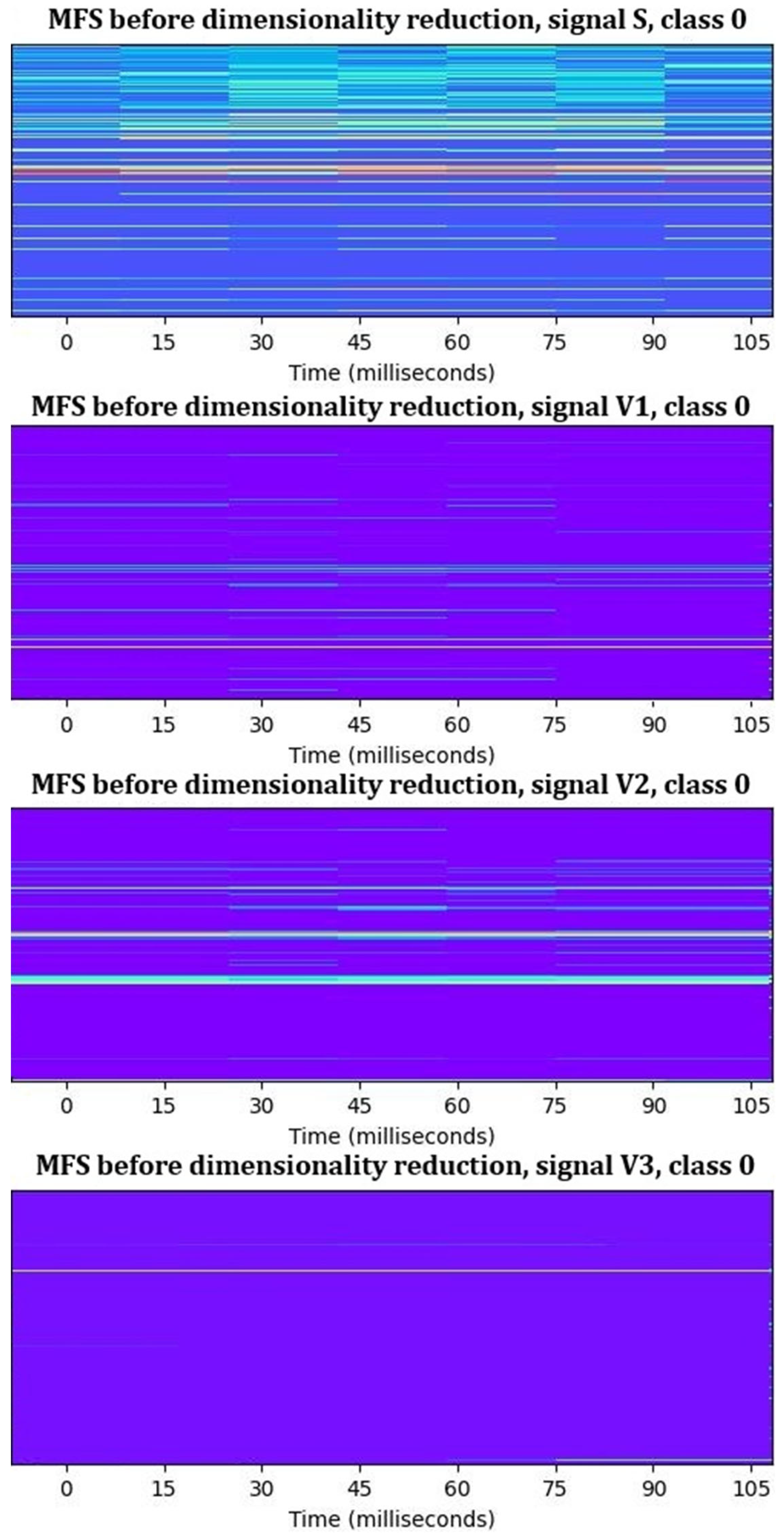
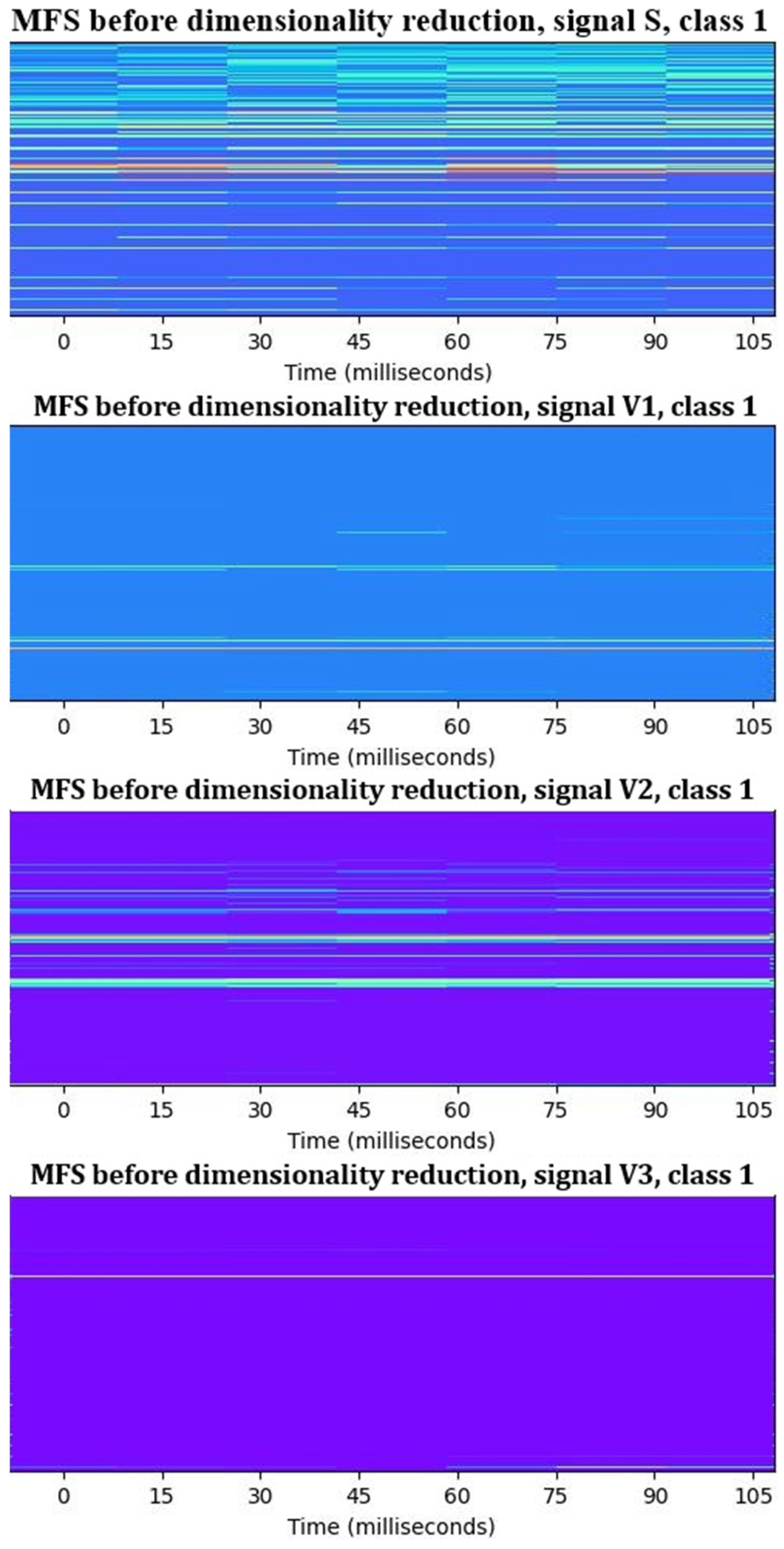
- Step 3: Feature reduction. In this step, a feature reduction process was applied to identify and remove non-informative frequency bands from the merged MFSs. Several statistical methods were used to evaluate the distribution and variability of values across each frequency band, including histogram analysis, standard deviation, peak analysis, and kurtosis assessment. Frequency bands were classified as non-informative and excluded from further analysis based on the following criteria:
- Low variance: Bands with values confined to a narrow range (e.g., all values falling within a single histogram bin) and exhibiting very low standard deviation were considered uninformative. Such low variability is typically associated with background noise or redundant data that contribute minimally to classification accuracy. This principle is widely supported in the feature selection literature, where low-variance features are routinely filtered out to improve learning performance and generalization ability [35,36].
- Lack of multimodality: Bands with distributions showing only one prominent peak or no significant peaks were assumed to lack distinctive features. Informative spectral regions, especially in fault diagnosis tasks, often exhibit multimodal behaviour due to the presence of multiple signal patterns or transient components. This behaviour has been observed in fault analysis using wavelet transforms and is emphasized in machine health monitoring literature [37,38].
- Low kurtosis (<3): Bands with a kurtosis value below 3 were identified as statistically flat (platykurtic), indicating the absence of outliers or sharp peaks. Such distributions generally lack impulsive components, which are important indicators of mechanical faults in vibration and acoustic signals. The threshold of kurtosis <3 was chosen based on standard statistical definitions [39,40] and reinforced by prior studies in predictive maintenance and condition monitoring [41,42]. Although not universally prescriptive, this threshold was also verified empirically in our study bands, as kurtosis values above 3 were more frequently observed to contain features contributing to successful fault classification, while those below this threshold consistently lacked discriminative power.
- 4.
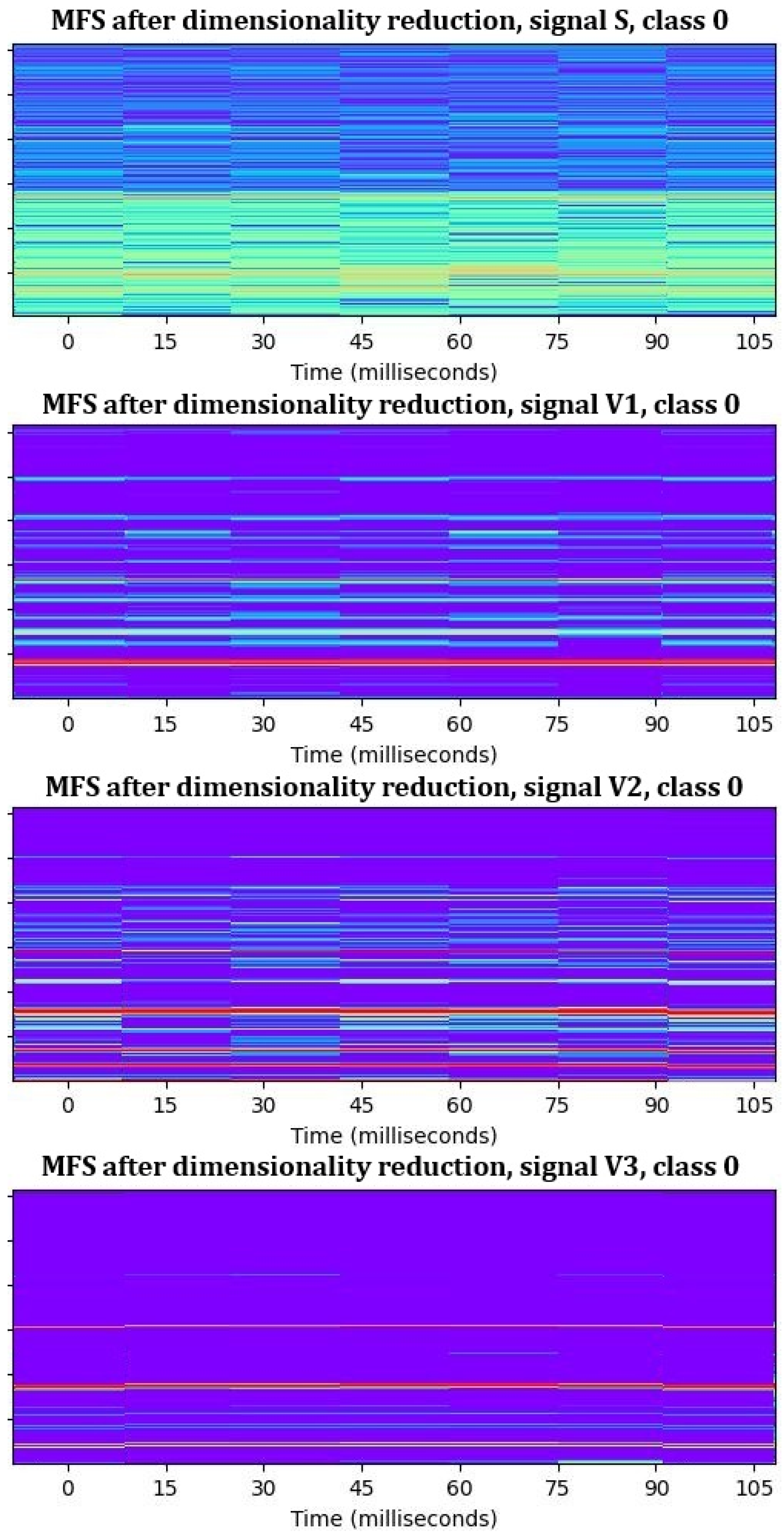
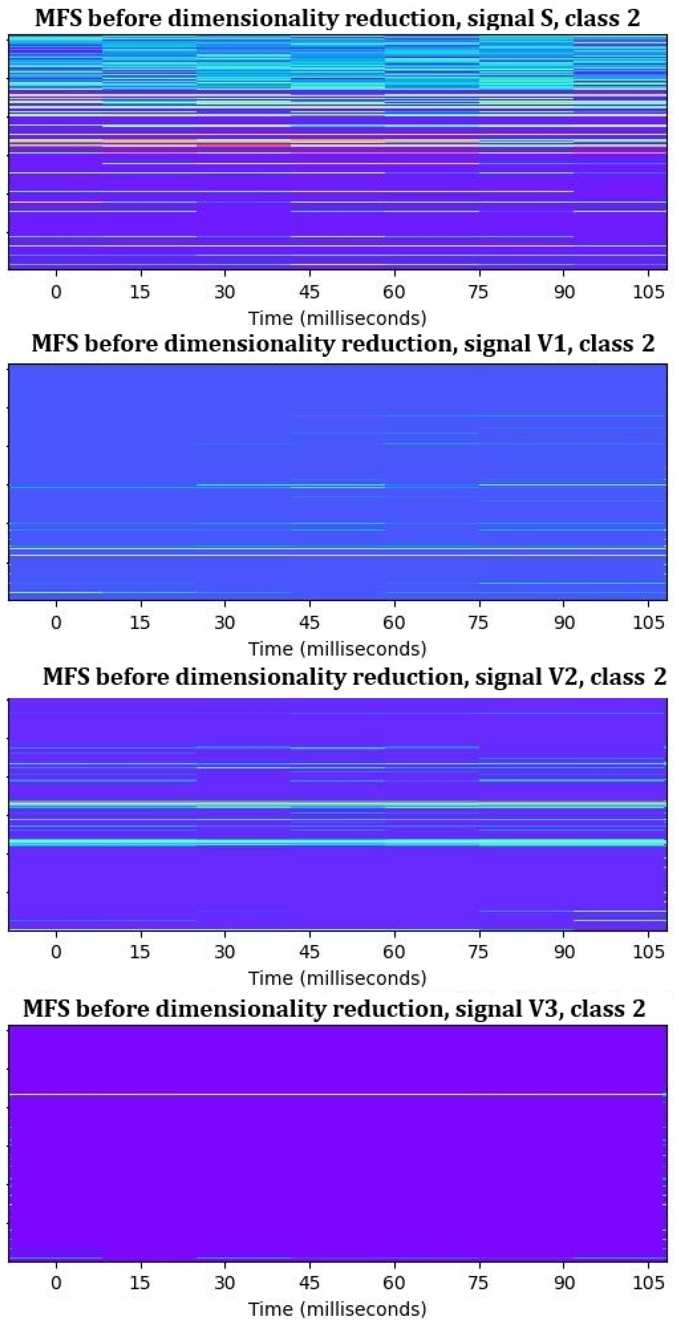
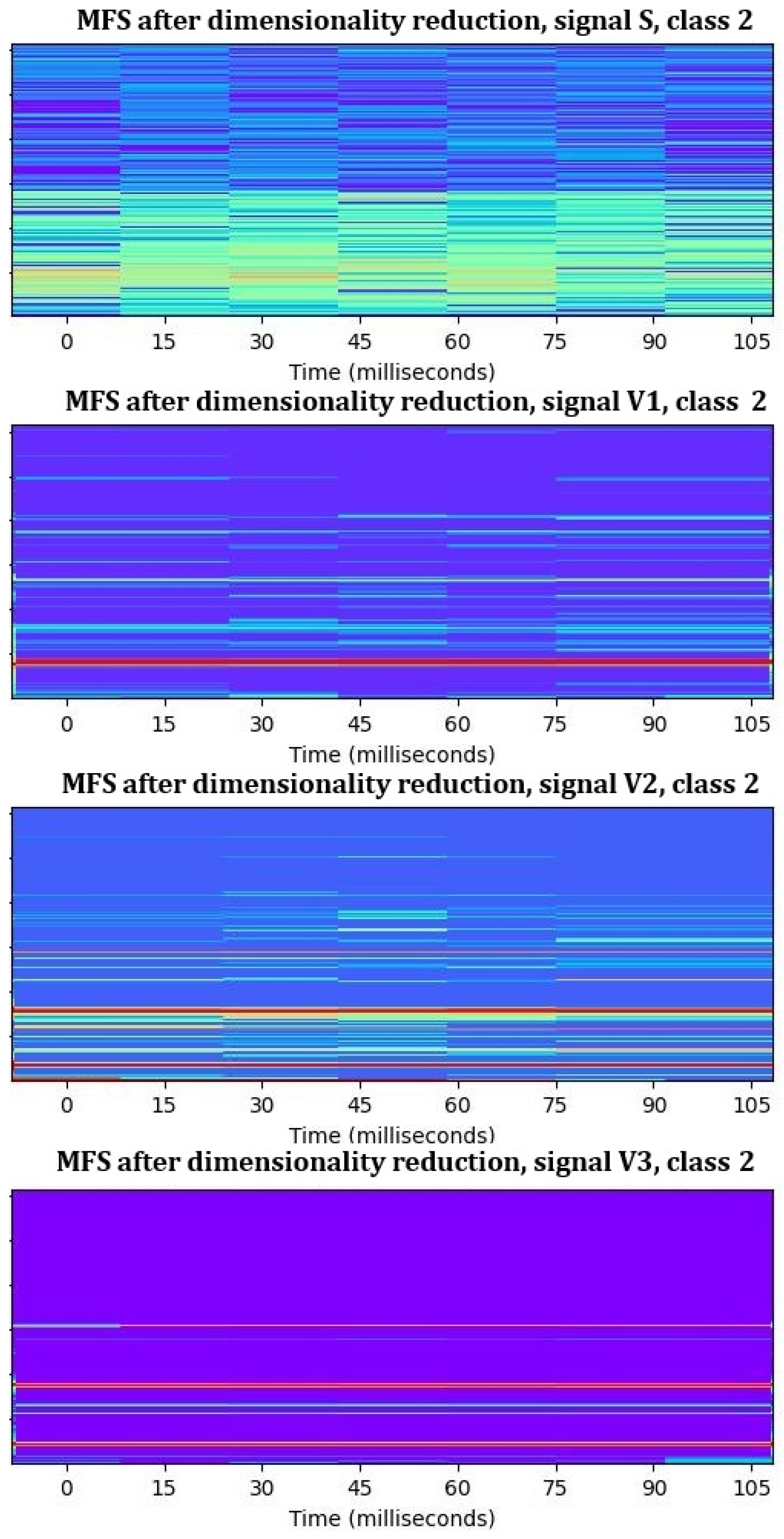
- Step 4: Creating new MFSs with only informative frequency bands. From the MFSs from step 1 we eliminated non-informative frequency bands, which were detected as non-informative after step 3. For each signal, we obtained a new dataset of reduced features for each motor, as shown in Table 5. These MFSs with reduced datasets (Figure 9) were used in continuing work.
- 5.
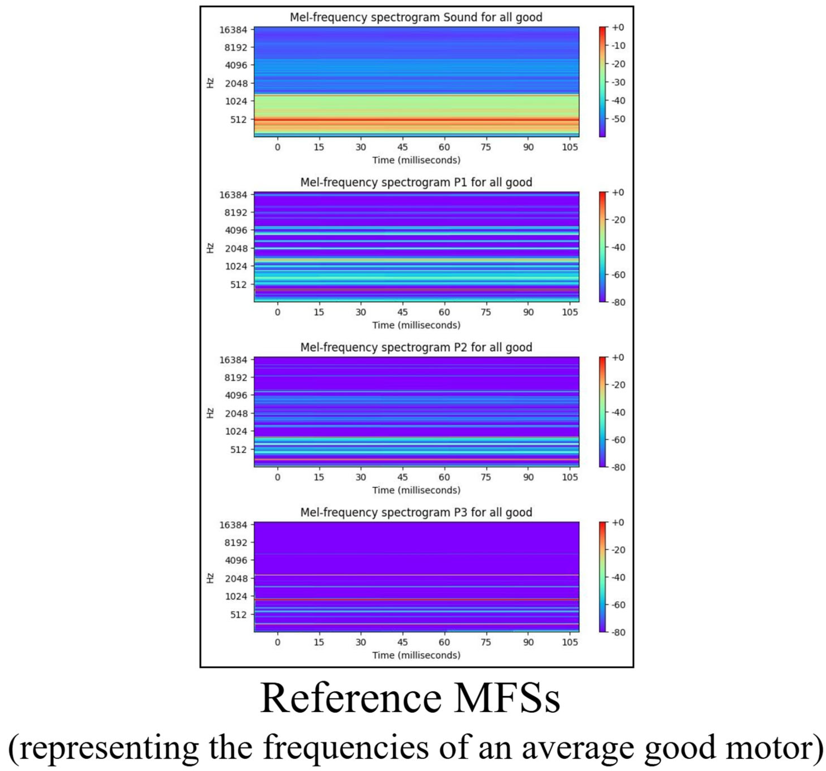
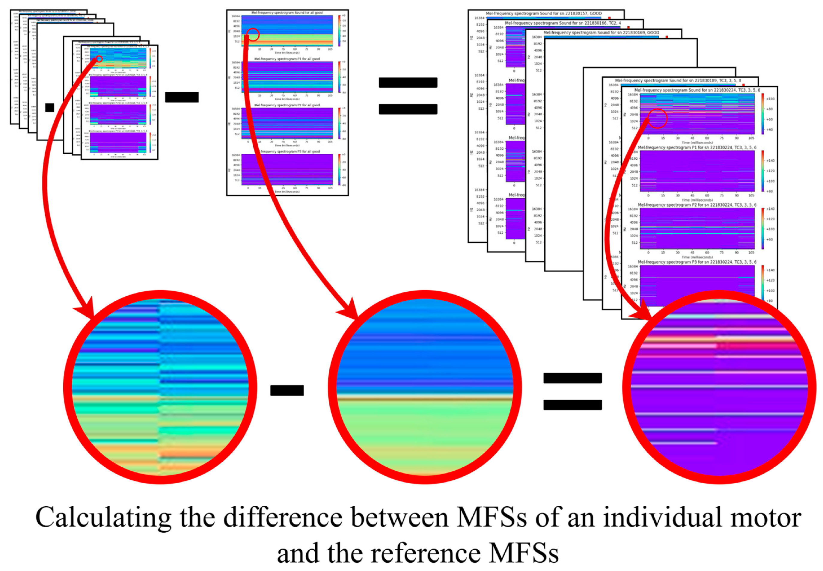
- Step 5: Creating the reference MFSs. Next, we selected all MFSs of good motors (class 0). From this group, we calculated an average MFS for each signal. These MFSs represent the typical time–frequency characteristics of non-faulty motors and serve as a baseline profile of a healthy motor. These average MFSs, illustrated in Figure 10, are also referred to as reference MFSs. This step was critical for step 6 where a direct comparison of the MFSs of each individual motor to the reference good motor was performed.
- 6.
- Step 6: Comparing MFSs of an individual motor to reference MFSs. The MFSs of each individual motor from step 4 were compared to the reference MFSs, as shown in Figure 11, and explained with (1). The comparison results reveal the difference between the individual motor and the normal state. This approach allowed for an easy identification of the time–frequency regions that differ from normal behaviour. This difference was used in further machine learning processes. This method is quite common in anomaly detection when fault data are sparse or highly imbalanced. Usually, it simplifies the interpretability of the model and increases the robustness of the classification. This approach also enabled more sensitive and targeted fault detection [43,44].
5. Neural Network Architecture and Training
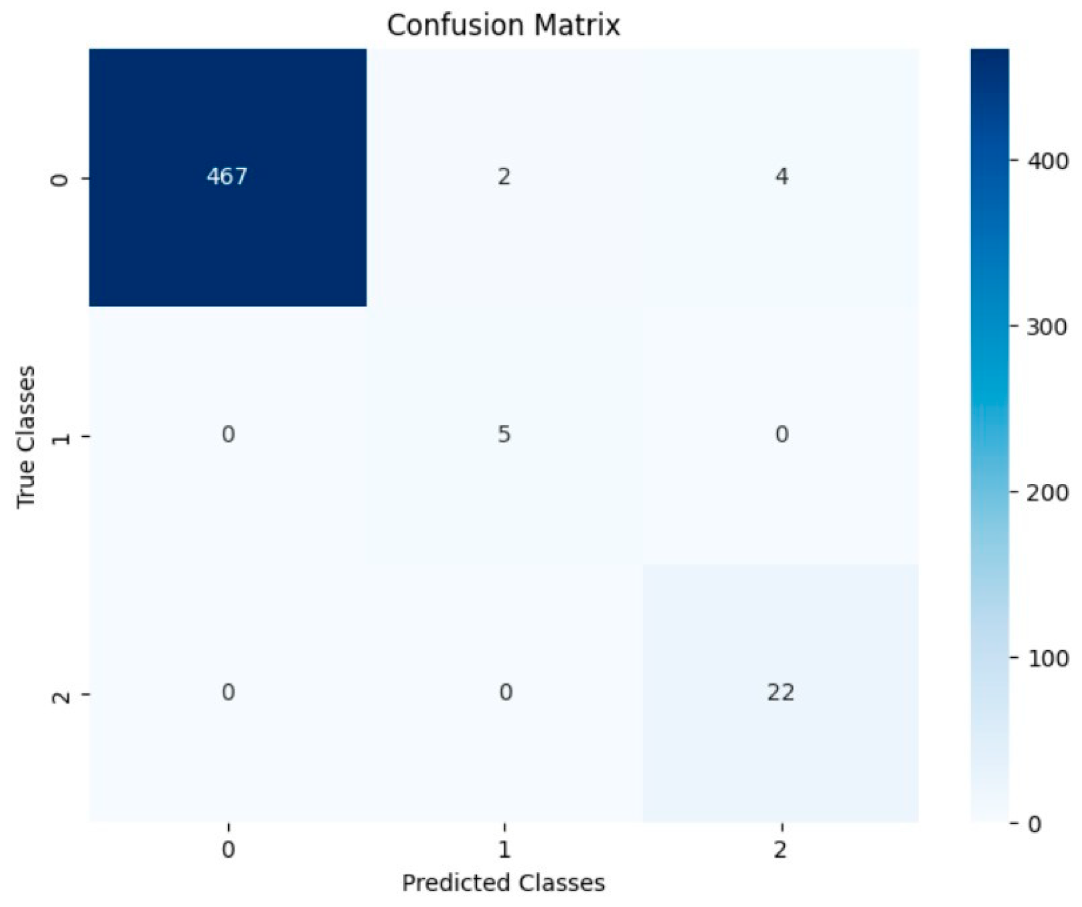
6. Results
- Precision—the proportion of motors classified into a class that truly belong to that class;
- Recall—the proportion of motors of a given class that were correctly identified;
- F1 score—the harmonic mean of precision and recall, offering a balanced view of both metrics;
- Support—the number of motor instances per class;
- Accuracy—the overall percentage of correct predictions across all classes;
- Macro average—the unweighted average of precision, recall, and F1 score across all classes (not accounting for class imbalance);
- Weighted average—The average of precision, recall, and F1 score across all classes (weighted by the number of instances per class, thus incorporating class imbalance).
7. Conclusions
Author Contributions
Funding
Data Availability Statement
Conflicts of Interest
Abbreviations
| EoL | End-of-Line |
| BLDC | Brushless DC |
| BiGRU | Bidirectional Gated Recurrent Unit |
| CNN | Convolutional Neural Network |
| CSRM-MIM | Catenary Support Rod area Masked Image Modelling |
| FENet | Focusing Enhanced Network |
| LRP | Layer-wise Relevance Propagation |
| MFS | Mel-Frequency Spectrogram |
| PINNs | Physics-Informed Neural Networks |
| SVM | Support Vector Machines |
| STFT | Short-Time Fourier Transform |
| TC1 | Test Cell 1 |
| TC2 | Test Cell 2 |
| TC3 | Test Eell 3 |
| t-SNE | t-distributed Stochastic Neighbour Embedding |
| XAI | Explainable AI |
References
- Benko, U.; Petrovčič, J.; Mussiza, B.; Juričić, Đ. A System for Automated Final Quality Assessment in the Manufacturing of Vacuum Cleaner Motors. IFAC Proc. Vol. 2008, 41, 7399–7404. [Google Scholar] [CrossRef]
- Juričić, Ð.; Petrovčič, J.; Benko, U.; Musizza, B.; Dolanc, G.; Boškoski, P.; Petelin, D. End-Quality Control in the Manufacturing of Electrical Motors. In Case Studies in Control: Putting Theory to Work; Springer: London, UK, 2013; pp. 221–256. [Google Scholar]
- Domel. About Us. Domel d. o. o. Available online: https://www.domel.com/about-us (accessed on 15 May 2025).
- Benko, U.; Petrovčič, J.; Juričić, Đ. In-depth fault diagnosis of small universal motors based on acoustic analysis. IFAC Proc. Vol. 2005, 38, 323–328. [Google Scholar] [CrossRef]
- Mlinarič, J.; Pregelj, B.; Boškoski, P.; Dolanc, G.; Petrovčič, J. Optimization of reliability and speed of the end-of-line quality inspection of electric motors using machine learning. Adv. Prod. Eng. Manag. 2024, 19, 183–196. [Google Scholar] [CrossRef]
- Boškoski, P.; Petrovčič, J.; Musizza, B.; Juričić, Đ. An end-quality assessment system for electronically commutated motors based. Expert Syst. Appl. 2011, 38, 13816–13826. [Google Scholar]
- Ribeiro, R.F.J.; Areias, I.A.D.S.; Mendes Campos, M.; Teixeira, C.E.; Silva, B.D.; Gomes, G.F. Fault detection and diagnosis in electric motors using 1d convolutional neural networks with multi-channel vibration signals. Measurement 2022, 190, 110759. [Google Scholar] [CrossRef]
- Fahad, A.; Luo, S.; Zhang, H.; Shaukat, K.; Yang, G.; Wheeler, C.A.; Chen, Z. A Brief Review of Acoustic and Vibration Signal-Based Fault Detection for Belt Conveyor Idlers Using Machine Learning Models. Sensors 2023, 23, 1902. [Google Scholar] [CrossRef]
- Zhang, W.; Peng, G.; Li, C.; Chen, Y.; Zhang, Z. A New Deep Learning Model for Fault Diagnosis with Good Anti-Noise and Domain Adaptation Ability on Raw Vibration Signals. Sensors 2017, 17, 425. [Google Scholar] [CrossRef]
- Janssens, O.; Slavkovikj, V.; Vervisch, B.; Stockman, K.; Loccufier, M.; Verstockt, S.; Van de Walle, R.; Van Hoecke, S. Convolutional Neural Network Based Fault Detection for Rotating Machinery. J. Sound Vib. 2016, 377, 331–345. [Google Scholar] [CrossRef]
- Ye, L.H.; Xue, M.; Cheng, L.W. Rotating Machinery Fault Diagnosis Method by Combining Time-Frequency Domain Features and CNN Knowledge Transfer. Sensors 2021, 21, 8168. [Google Scholar] [CrossRef]
- Yang, H.; Liu, Z.; Ma, N.; Wang, X.; Liu, W.; Wang, H.; Zhan, D.; Hu, Z. CSRM-MIM: A Self-Supervised Pre-training Method for Detecting Catenary Support Components in Electrified Railways. IEEE Trans. Transp. Electrif. 2025. [Google Scholar] [CrossRef]
- Yan, J.; Cheng, Y.; Zhang, F.; Zhou, N.; Wang, H.; Jin, B.; Wang, M.; Zhang, W. Multimodal Imitation Learning for Arc Detection in Complex Railway Environments. IEEE Trans. Instrum. Meas. 2025, 74, 1–13. [Google Scholar] [CrossRef]
- Chu, W.; Wang, H.; Song, Y.; Liu, Z. FENet: A Physics-Informed Dynamics Prediction Model of Pantograph-Catenary Systems in Electric Railway. IET Intell. Transp. Syst. 2025, 19, e70059. [Google Scholar] [CrossRef]
- Domel. Domel 759. Domel d. o. o. Available online: https://www.domel.com/product/759-bypass-low-voltage-high-efficiency-99 (accessed on 22 May 2025).
- Davis, S.B.; Mermelstein, P. Comparison of parametric representations for monosyllabic word recognition in continuously spoken sentences. IEEE Trans. Acoust. Speech Signal Process. 1980, 28, 357–366. [Google Scholar] [CrossRef]
- Logan, B. Mel frequency cepstral coefficients for music modeling. In Proceedings of the International Symposium on Music Information Retrieval (ISMIR), Cambridge, UK, 23–25 October 2000. [Google Scholar]
- Zavrtanik, V.; Marolt, M.; Kristan, M.; Skočaj, D. Anomalous Sound Detection by Feature-Level Anomaly Simulation. In Proceedings of the International Conference on Acoustics, Speech and Signal Processing, Seoul, Republic of Korea, 14–19 April 2024; IEEE: Piscataway, NJ, USA, 2024. [Google Scholar]
- Zhang, Y.; Li, X.; Gao, L.; Chen, W.; Li, P. Intelligent fault diagnosis of rotating machinery using a new ensemble deep auto-encoder method. Measurement 2020, 151, 107232. [Google Scholar] [CrossRef]
- Zhang, X.; Wang, L.; Xu, X.; Tang, J. Fault diagnosis of rotating machinery using deep convolutional neural networks with wide first-layer kernels. Knowl. Based Syst. 2019, 165, 105–114. [Google Scholar]
- Li, X.; Zhang, W.; Ding, Q.; Sun, J.-Q. Intelligent fault diagnosis of rotating machinery using deep wavelet auto-encoders. Mech. Syst. Signal Process. 2018, 2018, 204–216. [Google Scholar]
- Verstraete, D.; Ferrada, A.; Droguett, E.L.; Meruane, V.; Modarres, M. Deep Learning Enabled Fault Diagnosis Using Time-Frequency Image Analysis of Rolling Element Bearings. Shock. Vib. 2017, 2017, 5067651. [Google Scholar] [CrossRef]
- Liu, R.; Yang, B.; Zio, E.; Chen, X. Artificial intelligence for fault diagnosis of rotating machinery: A review. Mech. Syst. Signal Process. 2018, 108, 33–47. [Google Scholar] [CrossRef]
- Verstraete, D.; Ferrada, P.; Droguett, E.L.; Meruane, V.; Modarres, M. Deep learning enabled fault diagnosis using time-frequency image analysis of vibration signals for rotating machinery. Mech. Syst. Signal Process. 2018, 102, 360–377. [Google Scholar]
- Zhang, R.; Pan, J.; Wang, Z. Fault diagnosis model for rotating machinery using a novel image representation of vibration signal and convolutional neural network. Measurement 2019, 146, 305–311. [Google Scholar]
- Cho, K.; Merrienboer, B.V.; Gulcehre, C.; Bougares, B.D.F.; Schwenk, H.; Bengio, Y. Learning Phrase Representations using RNN Encoder-Decoder for Statistical Machine Translation. In Proceedings of the Empirical Methods in Natural Language Processing, Doha, Qatar, 25–29 October 2014. [Google Scholar]
- Zhao, Z.; Chen, W.; Wu, X.; Chen, C.Y.; Liu, J. LSTM network: A deep learning approach for short-term traffic forecast. IET Intell. Transp. Syst. 2017, 108, 68–75. [Google Scholar] [CrossRef]
- Liu, Y.; Wang, S.; Zhang, G. A novel fault diagnosis method based on CNN-BiGRU and improved spectrogram image of vibration signal. IEEE Access 2020, 8, 133885–133896. [Google Scholar]
- Tang, T.; Zhang, J.; He, Z. Bearing fault diagnosis using CNN-BiGRU network with time-frequency representation. Mech. Syst. Signal Process. 2020, 143. [Google Scholar]
- Wang, Z.; Liu, J.; Gu, F.; Ball, A. A CNN-BiGRU based method for rotating machinery fault diagnosis using time-frequency images. Sensors 2020, 20. [Google Scholar]
- Feng, Z.; He, W.; Qin, Y.; Ma, X. Rotating machinery fault diagnosis using hybrid deep neural networks with raw vibration signals. IEEE Trans. Ind. Electron. 2020, 67, 4143–4153. [Google Scholar]
- Kong, Q.; Xu, Y.; Wang, W.; Plumbley, M.D. Sound event detection of weakly labelled data with CNN-Transformer and Automatic Threshold Optimization. IEEE/ACM Trans. Audio Speech Lang. Process. 2020, 28, 2450–2460. [Google Scholar] [CrossRef]
- Xia, M.; Zhao, R.; Yan, R.; Zhang, S. Fault diagnosis for rotating machinery using multiple sensors and convolutional neural networks. IEEE/ASME Trans. Mechatron. 2020, 25, 853–862. [Google Scholar] [CrossRef]
- McFee, B.; Raffel, C.; Liang, D.; Ellis, D.P.; McVicar, M.; Battenberg, E.; Nieto, O. librosa: Audio and Music Signal Analysis in Python. In Proceedings of the 14th Python in Science Conference, Austin, TX, USA, 6–12 July 2015. [Google Scholar]
- Hyvärinen, A.; Karhunen, J.; Oja, E. Independent Component Analysis; Wiley-Interscience: New York, NY, USA, 2001. [Google Scholar]
- Guyon, I.; Elisseeff, A. An introduction to variable and feature selection. J. Mach. Learn. Res. 2003, 3, 1157–1182. [Google Scholar]
- Yan, R.; Gao, R.X.; Chen, X. Wavelets for fault diagnosis of rotary machines: A review with applications. Signal Process. 2014, 96, 1–15. [Google Scholar] [CrossRef]
- Tavner, P.J.; Ran, L.; Penman, J.; Sedding, H. Condition Monitoring of Rotating Electrical Machines; IET: London, UK, 2008. [Google Scholar]
- Antoni, J. Fast computation of the kurtogram for the detection of transient faults. Mech. Syst. Signal Process. 2007, 21, 108–124. [Google Scholar] [CrossRef]
- Wyłomańska, A. Statistical tools for anomaly detection as a part of predictive maintenance in the mining industry. Eur. Math. Soc. Mag. 2022, 124, 4–15. [Google Scholar] [CrossRef]
- Wang, W.; Tse, P.W.; Liu, Z. A Review of Spectral Kurtosis for Bearing Fault Detection and Diagnosis. Mech. Syst. Signal Process. 2021, 147. [Google Scholar]
- Radosz, A.; Zimroz, R.; Bartelmus, W. Identification of Local Damage in Gearboxes Based on Spectral Kurtosis and Selected Condition Indicators. J. Vibroengineering 2017, 19, 2950–2963. [Google Scholar]
- Jia, F.; Lei, Y.; Lin, J.; Zhou, X.; Lu, N. Deep neural networks: A promising tool for fault characteristic mining and intelligent diagnosis of rotating machinery with massive data. Mech. Syst. Signal Process. 2016, 72–73, 303–3015. [Google Scholar] [CrossRef]
- Zhao, R.; Yan, R.; Chen, X.; Mao, K.; Wang, P.; Gao, R.X. Deep learning and its applications to machine health monitoring. Mech. Syst. Signal Process. 2019, 115, 213–237. [Google Scholar] [CrossRef]
- Snoek, J.; Larochelle, H.; Adams, R.P. Practical Bayesian Optimization of Machine Learning Algorithm. Adv. Neural Inf. Process. Syst. 2012, 25, 2951–2959. [Google Scholar]
- Pan, S.J.; Yang, Q. A Survey on Transfer Learning. IEEE Trans. Knowl. Data Eng. 2010, 22, 1345–1359. [Google Scholar] [CrossRef]
- Weiss, K.; Khoshgoftaar, T.M.; Wang, D. A survey of transfer learning. Big Data 2016, 3, 9. [Google Scholar] [CrossRef]
- Piczak, K.J. Environmental sound classification with convolutional neural networks. In Proceedings of the IEEE International Workshop on Machine Learning for Signal Processing, Boston, MA, USA, 17–20 September 2015. [Google Scholar]
- Marchi, E.; Vesperini, F.; Eyben, F.; Squartini, S.; Schuller, B. A novel approach for automatic acoustic novelty detection using a denoising autoencoder with bidirectional LSTM neural networks. In Proceedings of the ICASSP 2015—IEEE International Conference on Acoustics, Speech and Signal Processing, Brisbane, Australia, 19–24 April 2015. [Google Scholar]


| Measurement Status | Features | Diagnostic Result |
|---|---|---|
| Completed | All features are within specified ranges. | Good |
| One or more features are outside specified range. | Bad | |
| Not completed | Missing features. | Undefined |
| Class | Number of Motors | Part [%] |
|---|---|---|
| 0 | 1422 | 94.49 |
| 1 | 16 | 1.06 |
| 2 | 67 | 4.45 |
| Name of Parameter | Brief Explanation | Value |
|---|---|---|
| sampling rate | The sampling frequency of raw input data [Hz], determined by hardware. | 60,000 |
| nfft | The length of the FFT window; defines frequency resolution. Set empirically. | 2000 |
| win_length | The length of the window for FFT analysis (same or smaller than nfft). Set equal to nfft for maximum frequency detail without truncation. | 2000 |
| hop_length | The number of samples between windows (hop); controls the time resolution of the MFS. Tuned empirically to balance the resolution and training stability. | 1000 |
| centre | The positioning of the window (symmetric analysis). | True |
| pad_mode | How the signal at the edge is completed. “Reflect” mirrors the signal at the edges, minimizing boundary artefacts and preserving continuity [34]. | Reflect |
| power | The exponent magnitude of the Mel-frequency spectrogram (1—energy and 2—power). | 2 |
| n_mels | The number of Mel-frequency bands. Chosen empirically. | 2048 |
| fmin | Low frequency limit; set by experts from the industrial partner. | 20 |
| fmax | High frequency limit; set by experts from the industrial partner. | 18,000 |
| Signal | Number of Frequency Bands Before Reduction | Number of Frequency Bands After Reduction | Part of Informative Frequency Bands |
|---|---|---|---|
| S | 2048 | 678 | 0.33 |
| V1 | 2048 | 381 | 0.19 |
| V2 | 2048 | 701 | 0.34 |
| V3 | 2048 | 709 | 0.35 |
| Together | 8192 | 2469 | 0.30 |
| Signal | Size of Dataset [Features × Time Frames] |
|---|---|
| S | 678 × 7 |
| V1 | 381 × 7 |
| V2 | 701 × 7 |
| V3 | 709 × 7 |
| Layer (Type) | Output Shape | Details |
|---|---|---|
| Input | (None, 7, 2469, 1) | Size of MFS |
| First Conv2D | (None, 7, 2469, 32) | First 2D convolutional layer with 32 filters, ReLU activation, and kernel size (7 × 7) |
| First Batch Normalization | (None, 7, 2469, 32) | Normalizes activations, improves training stability |
| First Max Pooling 2D | (None, 3, 1234, 32) | Down samples feature maps by 2 × 2 |
| First Dropout | (None, 3, 1234, 32) | Prevents overfitting, dropout value 0.5 |
| Second Conv2D | (None, 3, 1234, 64) | Second 2D convolutional layer with 64 filters, ReLU activation, and kernel size (7 × 7) |
| Second Batch Normalization | (None, 3, 1234, 64) | Further normalization post-convolution |
| Second Max Pooling 2D | (None, 1, 617, 64) | Further spatial reduction |
| Second Dropout | (None, 1, 617, 64) | Additional dropout, dropout value 0.5 |
| Reshape | (None, 1, 39,488) | Flattening spatial data into time sequence |
| First Bidirectional BiGRU | (None, 1, 128) | First BiGRU layer (2 × 64 units) capturing bidirectional context |
| Second Bidirectional BiGRU | (None, 128) | Second BiGRU layer (2 × 64 units), flattening to vector |
| First Dense | (None, 64) | Fully connected layer |
| Third Dropout | (None, 64) | Final dropout before output, dropout value 0.4 |
| Second Dense | (None, 3) | Final layer for 3-class classification (Softmax) |
| Class | Precision | Recall | F1 Score | Support |
|---|---|---|---|---|
| 0 | 1 [0.99, 1] | 0.99 [0.98, 1] | 0.99 [0.98, 1] | 473 |
| 1 | 0.71 [0.55, 1] | 1 [0.80, 1] | 0.83 [0.67, 1] | 5 |
| 2 | 0.85 [0.75, 1] | 1 [0.92, 1] | 0.92 [0.84, 1] | 22 |
| Metrics | Precision | Recall | F1 Score | Support |
|---|---|---|---|---|
| Accuracy | 0.99 [0.98, 1] | 500 | ||
| Macro average | 0.85 [0.75, 0.95] | 1 [0.99, 1] | 0.91 [0.82, 0.98] | 500 |
| Weighted average | 0.99 [0.98, 1] | 0.99 [0.98, 1] | 0.99 [0.98, 1] | 500 |
Disclaimer/Publisher’s Note: The statements, opinions and data contained in all publications are solely those of the individual author(s) and contributor(s) and not of MDPI and/or the editor(s). MDPI and/or the editor(s) disclaim responsibility for any injury to people or property resulting from any ideas, methods, instructions or products referred to in the content. |
© 2025 by the authors. Licensee MDPI, Basel, Switzerland. This article is an open access article distributed under the terms and conditions of the Creative Commons Attribution (CC BY) license (https://creativecommons.org/licenses/by/4.0/).
Share and Cite
Mlinarič, J.; Pregelj, B.; Dolanc, G. End-of-Line Quality Control Based on Mel-Frequency Spectrogram Analysis and Deep Learning. Machines 2025, 13, 626. https://doi.org/10.3390/machines13070626
Mlinarič J, Pregelj B, Dolanc G. End-of-Line Quality Control Based on Mel-Frequency Spectrogram Analysis and Deep Learning. Machines. 2025; 13(7):626. https://doi.org/10.3390/machines13070626
Chicago/Turabian StyleMlinarič, Jernej, Boštjan Pregelj, and Gregor Dolanc. 2025. "End-of-Line Quality Control Based on Mel-Frequency Spectrogram Analysis and Deep Learning" Machines 13, no. 7: 626. https://doi.org/10.3390/machines13070626
APA StyleMlinarič, J., Pregelj, B., & Dolanc, G. (2025). End-of-Line Quality Control Based on Mel-Frequency Spectrogram Analysis and Deep Learning. Machines, 13(7), 626. https://doi.org/10.3390/machines13070626