Determining Vibration Characteristics and FE Model Updating of Friction-Welded Beams

Abstract

This study aimed to investigate the dynamic characteristics of shafts joined by friction welding and to update their finite element models. The first five bending mode resonance frequencies, damping ratios, and mode shapes of SAE 304 steel beams, friction-welded at three different rotational speeds (1200, 1500, and 1800 rpm), were determined using the Experimental Modal Analysis method. This approach allowed for an examination of how the dynamic properties of friction-welded beams change at varying rotational speeds. A slight decrease in resonance frequency values was observed with the transition from lower to higher rotational speeds. The largest difference of 3.28% was observed in the first mode, and the smallest difference of 0.19% was observed in the second mode. Different trends in damping ratios were observed for different modes. In the first, second, and fourth modes, damping ratios tended to increase with increasing rotational speeds, while they tended to decrease in the third and fifth modes. The largest difference was calculated as 52.83% in the third vibration mode. However, no significant change in mode shapes was observed for different rotational speeds. Based on the examined Modal Assurance Criterion (MAC) results, cross-comparisons of the mode shapes obtained for all three different speeds yielded a minimum similarity of 93.8%, reaching up to 99.9%. For model updating, a Frequency Response Assurance Criterion (FRAC)-based method utilizing frequency response functions (FRFs) was employed. Initially, a numerical model of the welded shaft was created using MATLAB-R2015a, based on the Euler–Bernoulli beam theory. Since rotational coordinates were not used in the EMA analyses, static model reduction was performed on the numerical model to reduce the effect of rotational coordinates to translational coordinates. For model updating, experimentally obtained FRFs from EMA and FRFs from the numerical model were used. The equivalent modulus of elasticity and equivalent density of the friction weld region were used as updating parameters. Successful results were achieved by developing an algorithm that ensured the convergence of the numerical model’s FRFs and natural frequencies.

1. Introduction

Friction welding is a type of solid-state welding method that is widely used in engineering applications. In this welding method, two parts with the same or different material properties, usually cylindrical in shape, are brought together on the same axis and rotated to create friction heat at the contact point. This heat softens the metal, causing plastic deformation and allowing the contact surfaces of the parts to come together under applied pressure. Friction welding is a faster, more efficient, and more environmentally friendly joining method compared to traditional methods such as TIG, MIG, and MAG, since it does not require additional material or shielding gas during the welding process. In addition, it is widely used in sectors such as automotive, aviation, and energy, with its ability to join both the same and different types of metals and provides efficiency and flexibility in production by providing high-quality and durable connections.

In general, friction welding can be examined in two classes as Rotary Friction Welding and Linear Friction Welding. In Rotary Friction Welding applications, the two parts to be welded are placed on the same rotation axis and generally, materials with a circular cross-section shape are joined. While one of the parts is kept stationary, the other is rotated at a certain speed. The necessary heat is generated by the contact of the rotating part with the stationary part (Marimuthu et al. [1] and Anandaraj et al. [2]). In Linear Friction Welding, both parts move linearly and heat is generated as a result of friction on the contact surfaces; the joining process is performed thanks to this heat and the applied pressure. It is generally used in joining rectangular cross-sections and complex structured parts (Sing and Sharma [3] and Orlowska et al. [4]). Apart from this, many different friction welding applications are made, e.g., Friction Stir Welding, Friction Surfacing, Friction Plunge Welding, Friction Brazing, Friction Taper Stitch Welding, and Friction Seam Welding (Nicholas [5]). Friction welding is generally used quite widely in joining materials with similar mechanical properties; however, it can also yield quite successful results in joining different types of materials with different mechanical properties. It has been demonstrated by many researchers that many different types of materials such as copper and stainless steel (Kimura et al. [6]), titanium and stainless steel (Balasubramanian et al. [7]), and aluminum and stainless steel (Vyas et al. [8]) can be successfully joined by friction welding. In addition, the weldability of shape memory alloys by friction welding and the effects of graphene-reinforced alloys on friction welding performance have also been investigated (Albuquerque et al. [9] and Becheikh and Tashkandi [10]).

Numerical modeling of the friction welding process can provide great convenience in terms of evaluating the process and its effects (thermo-physical properties, microstructure, mechanical properties, etc.) without performing real welding (Bauarroudj et al. [11], Jedrasiak et al. [12] and Lei et al. [13]. In this way, studies can be carried out safely by taking the necessary precautions. In addition to the research carried out on these numerical models, some mechanical analysis and microstructure studies carried out experimentally should also be evaluated and these numerical models should be verified (Winiczenko and Skibicki [14]). Many parameters such as environmental conditions, rotation speed, pressure, material type, and interface temperature in friction welding applications have significant effects on welding performance (Wand et al. [15], Nagasankar at al. [16], Deepak et al [17], and Jeong et al. [18]). The microstructure formed in the weld zones of the materials is directly related to the mechanical properties of the welded structure (Waikwad et al. [19], Su et al. [20], Karadge et al. [21], and Reyes et al. [22]). Therefore, it is of great importance to know the thermal distribution and microstructure of the materials joined by friction welding according to the type of welding, welding parameters, and type of materials to be welded (Mani et al. [23], Zhao et al. [24], Xu et al. [25], and Geng et al. [26]). In order to obtain the best performance, the optimum values of these parameters should be optimized (Polami et al. [27] and Buzzatti et al. [28]). Numerical models of physical systems often fail to perfectly represent the real system due to various factors such as material imperfections, manufacturing tolerances and errors, and measurement uncertainties. In such cases, finite element model updating techniques are employed to refine the numerical model based on the real system’s behavior. Within the scope of structural dynamics, numerous model updating methods based on modal data are utilized. These include approaches rooted in force equilibrium, error matrix methods, control theory, energy principles, and sensitivity-based approaches (Chen and Wada [29] and Sidhu and Ewins [30]). Beyond these, various model updating techniques also exist that leverage time-domain data or directly employ frequency response functions (FRFs) (Gang et al. [31] and Yuen and Katafygiotis [32]). Methods relying on FRFs offer significant advantages in terms of practical applicability. This is primarily because the necessary FRFs can be directly obtained from the real system, eliminating the need for a prerequisite modal model.

Friction welding is widely used in areas where systems generally operate under dynamic effects, such as automotive, manufacturing, aviation, and maritime. Therefore, in addition to the mechanical strength, thermomechanical properties, and material microstructure studies of the structures joined by friction welding, it is very important to carefully consider their dynamic characteristics (resonance frequencies, damping ratios, and vibration mode shapes) so that these structures can operate safely under dynamic operating conditions. In addition, knowing the dynamic properties is also of great importance in the design phase of dynamic systems. Therewithal, its use in studies, e.g., design verification and FE model updating, provides great convenience to designers and researchers. In this study, the dynamic characteristics of beams connected with friction welding were obtained using the EMA method. In this context, the resonance frequencies, damping ratios, and vibration mode shapes of these structures were obtained. In addition, FE model of the beams connected with friction welding were updated using the EMA results. In this way, the dynamic behaviors of these structures can be observed on the updated numerical model and the necessary analyses can be made correctly on the updated FE model.

2. Materials and Methods

2.1. Friction Welding of Beams

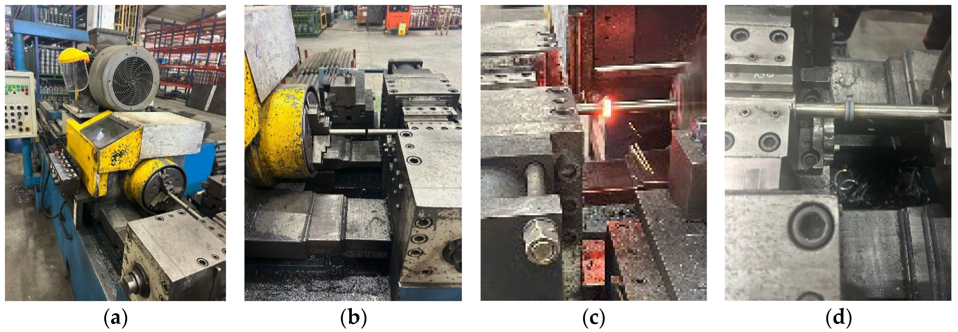
In this study, SAE 304 stainless steel (2 specimens of 300 mm lengths, 20 mm diameter, 7900 kg/m³ mass density, and 190 GPa modulus of elasticity) beams were joined by rotational friction welding. Friction welding was performed using a friction welding machine operated at different rotational speeds (1200, 1500 and 1800 rpm) and for constant shortening for each specimen as 6 mm (Figure 1).

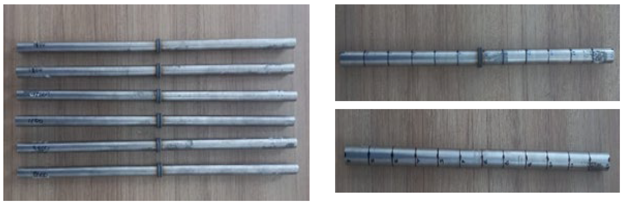
One of the beams was connected to the rotating part of the machine and the other was placed on the fixed center. The beams were brought into contact with each other and the machine was operated at the specified rotation speed to create friction heat. Then, after the specified pressure was created and the joint was achieved, the rotation of the machine with high brake power was stopped and the friction welding process was completed. Flash formation after welding was removed by turning and a constant diameter was obtained along the beam (Figure 2).

2.2. Experimental Modal Analysis

In this study, the Experimental Modal Analysis (EMA) method was used to determine the dynamic properties of friction-welded beams. In EMA, the structure is excited by measurable force and the responses of the structure to this exciting force are measured. With the linear relation of the input force and the output of the system, the FRFs, which are related to the dynamic characteristics of these systems (natural frequencies, damping ratios, and vibration mode shapes), are obtained. In addition, FRFs can also be used for structural modification and FE model updating.

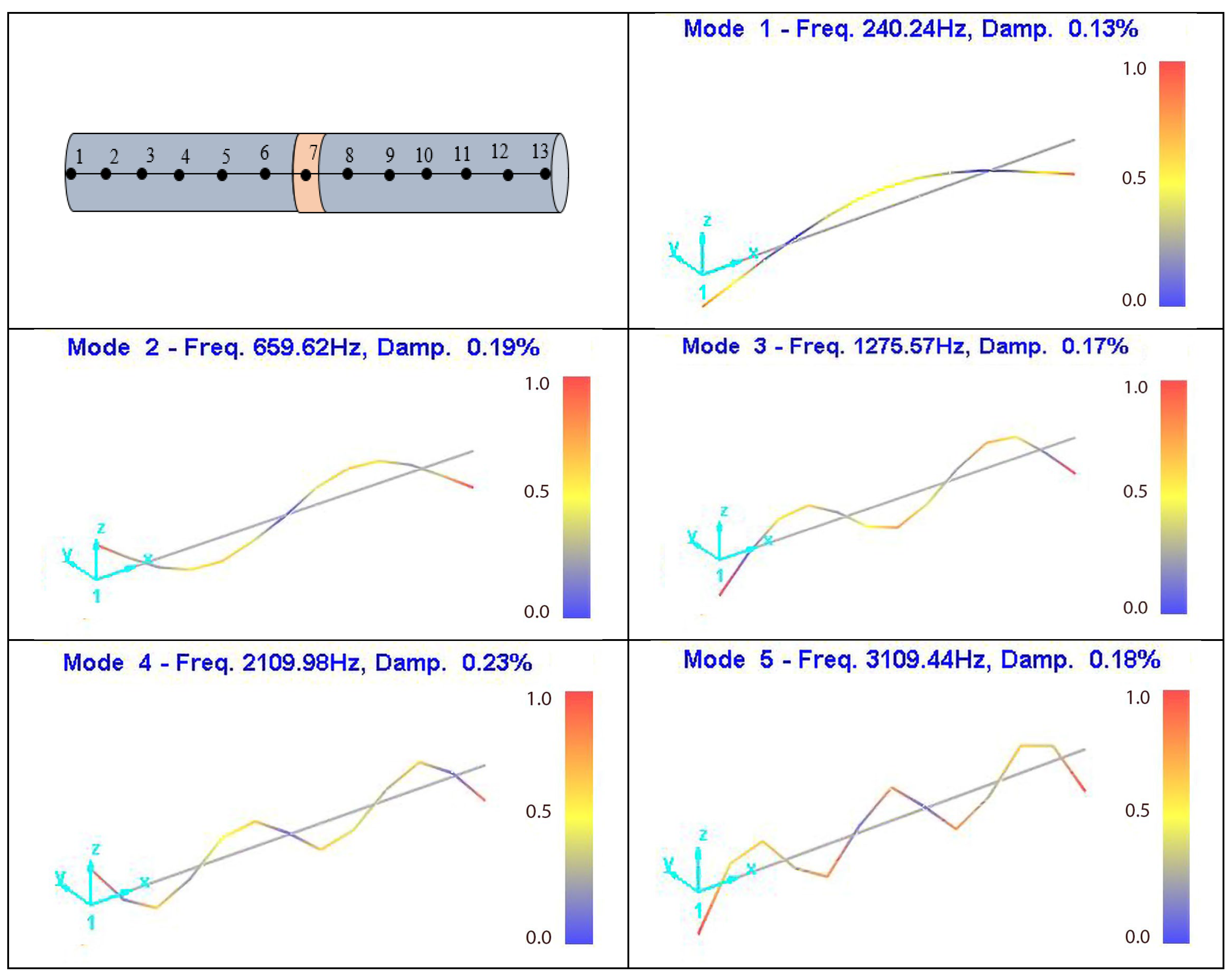
For EMA in this study, the friction-welded specimens were portioned into 12 intervals and for each specimen, 13 nodes were created as illustrated in Figure 3. The coordinate in the middle of the beam (node 7) belongs to the center of friction weld zone.

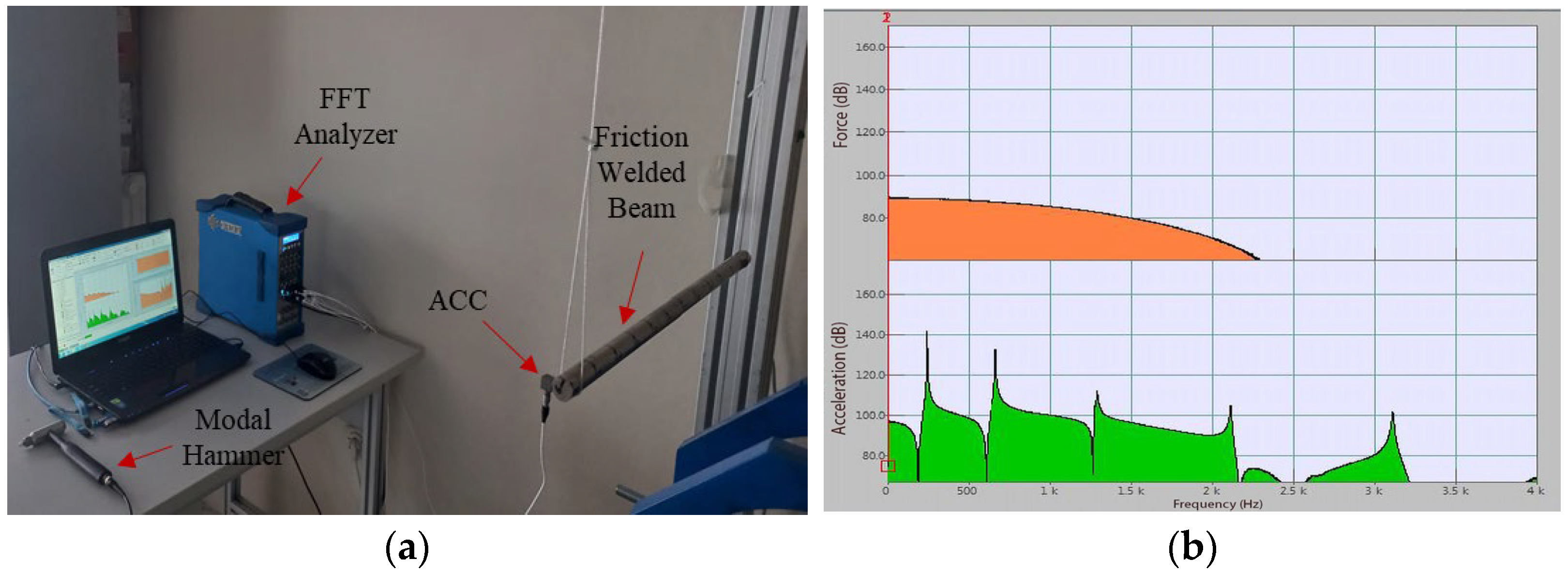
The EMA setup is shown in Figure 4. The prepared beams were hung to a stand using treads at each end of the beams and free vibration boundary condition was provided. To excite the specimens, a modal hammer (Kistler/9724A2000, Kistler Group, Winterthur, Switzerland) was used and to measure the responses, a single-axis ICP type accelerometer (Dytran/3097A2, Dytran Instruments Inc., Chatsworth, CA, USA) was used. The specimens were excited from the nodal points sequentially by making three hits for each node. The input forces and the output responses of the specimens were collected using the Oros/OR36 series vibration analyzer (OROS Group, Montbonnot Saint Martin, France). Fast Fourier Transform (FFT) was performed and then analyzed with the OROS NVGate analysis program.

An illustration of the EMA test and a measurement example is given in Figure 5.

The required analysis settings were made for a frequency bandwidth covering the first 5 bending vibration modes of the specimens. Nyquist criterion was ensured by taking the sampling frequency to be twice the largest frequency in the examined frequency range. It was not necessary to use any windowing function in the vibration analysis process due to the amplitude of the time response obtained when the accelerometer reached zero within the measured time, so no additional damping occurred. In addition, checking tests such as repeatability, reciprocity, and linearity were carried out to obtain more reliable results.

2.3. FE Modeling

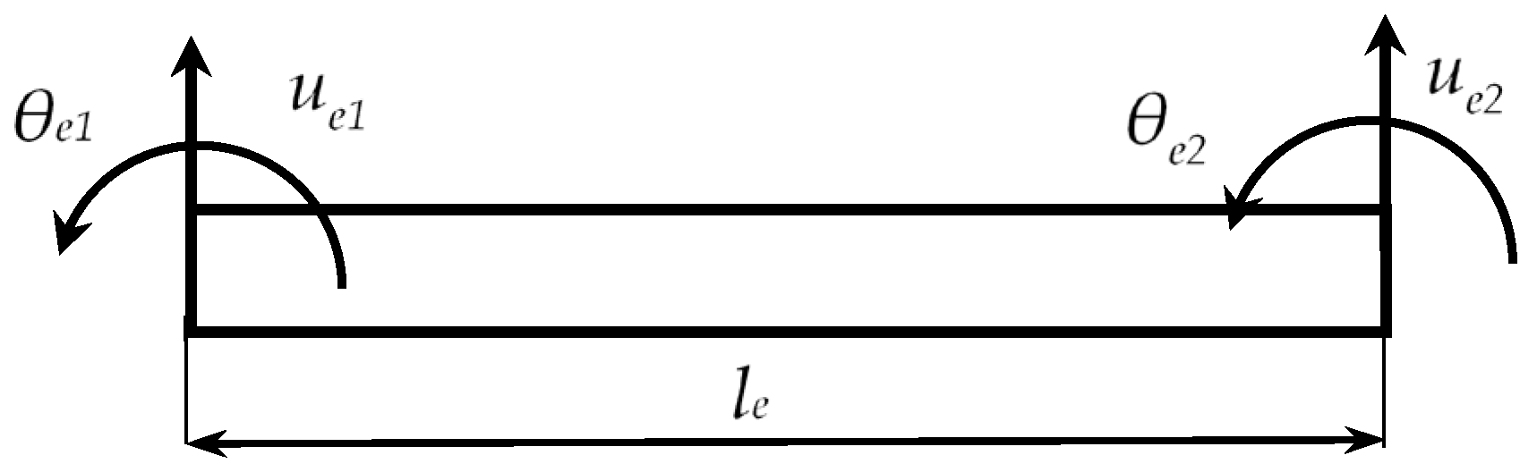
The friction-welded beam was modeled with the Euler–Bernoulli beam approach using MATLAB and the free bending vibrations in one plane were investigated. For such FE model, each node has 2 degrees of freedom, 1 translation, and 1 rotation (Figure 6).

The coordinates of the beam finite element can be written with Equation (1).

$$\left\{q_e\right\}={\left\{u_{e1},{\theta }_{e1},u_{e2},{\theta }_{e2}\right\}}^T$$

(1)

where u_e1, u_e2 and θ_e1, θ_e2 are the translational and the rotational coordinates, respectively. Each node has 2 and each beam finite element has a total of 4 degrees of freedom. The stiffness and mass matrices obtained for each beam finite element are given with Equations (2) and (3), respectively.

$${\left[k_s\right]}^{(i)}=\left[\begin{array}{cccc}{k}_{11}^{(i)}& \begin{array}{l}{k}_{12}^{(i)}\hfill \end{array}& k_{13}^{(i)}& k_{14}^{(i)}\\ k_{21}^{(i)}& k_{22}^{(i)}& k_{23}^{(i)}& k_{24}^{(i)}\\ k_{31}^{(i)}& k_{32}^{(i)}& k_{33}^{(i)}& k_{34}^{(i)}\\ k_{41}^{(i)}& k_{42}^{(i)}& k_{43}^{(i)}& k_{44}^{(i)}\end{array}\right]={\displaystyle \frac{E_i{I}_i}{l_i^3}}\left[\begin{array}{cccc}12& 6l_i& -12& 6l_i\\ 6l& {4l}_i^2& -6l_i& {2l}_i^2\\ -12& -6l_i& 12& -6l_i\\ 6l_i& {2l}_i^2& -6l_i& {4l}_i^2\end{array}\right](i=1,2,\dots ,n)$$

(2)

$${\left[m_s\right]}^{(i)}=\left[\begin{array}{cccc}{m}_{11}^{(i)}& \begin{array}{l}{m}_{12}^{(i)}\hfill \end{array}& m_{13}^{(i)}& m_{14}^{(i)}\\ m_{21}^{(i)}& m_{22}^{(i)}& m_{23}^{(i)}& m_{24}^{(i)}\\ m_{31}^{(i)}& m_{32}^{(i)}& m_{33}^{(i)}& m_{34}^{(i)}\\ m_{41}^{(i)}& m_{42}^{(i)}& m_{43}^{(i)}& m_{44}^{(i)}\end{array}\right]={\displaystyle \frac{{\rho }_i{A}_i{l}_i}{420}}\left[\begin{array}{cccc}156& 22l_i& 54& -13l_i\\ 22l_i& {4l}_i^2& 13l_i& {-3l}_i^2\\ 54& 13l_i& 156& -22l_i\\ -13l_i& {-3l}_i^2& -22l_i& {4l}_i^2\end{array}\right](i=1,2,\dots ,n)$$

(3)

In Equation (2), E_i, I_i, and l_i are the modulus of elasticity, moment of inertia, and the length of the beam elements, respectively, and [k_s]⁽ⁱ⁾ represents the stiffness matrix. In Equation (3), ρ_i, A_i, and [m_s]⁽ⁱ⁾ are the mass density, cross-section area, and the mass matrix of the beam element.

Using these element stiffness and mass matrices sequentially for all intervals of the beam, the global mass and stiffness matrices of the beam can be created and the equation of motion of the beam is obtained with Equation (4). By using Equation (4), the dynamic analysis can be made for the beam numerically.

$$\left[M\right]\left\{\ddot{q}\right\}+\left[K\right]\left\{q\right\}=\left\{F\right\}$$

(4)

The friction weld zone is modeled with a mass density ρ_w and modulus of elasticity E_w (Figure 7).

2.4. Model Reduction and FE Model Updating

In the calculation of dynamic properties obtained by EMA, excitation and response data can be acquired and utilized from a limited number of coordinates. Typically, single-axis excitation data at translational coordinates generated by a modal hammer or shaker, and single-axis response data at translational coordinates obtained by accelerometers, are employed. This is because exciting a system at rotational coordinates and measuring response data at these coordinates necessitate the use of economically unviable equipment. The exclusion of rotational coordinate data leads to discrepancies between the developed FE model and the experimental model. To compensate for these and similar issues, model reduction methods have been developed. These methods are based on the principle of constraining or eliminating certain coordinates and transferring their effects to selected coordinates. Static and dynamic model reduction techniques are widely used for this purpose (Guyan [33], Rouch and Kao [34], and Tiwari [35]). In this study, the dynamic effects at rotational coordinates of the developed FE model were reduced to translational coordinates using static model reduction.

For the dynamically expressed system in Equation (4), the mass, stiffness, and force terms can be rearranged and written as follows by separating them into sub-matrices and vectors for secondary and primary coordinates:

$$\left[\begin{array}{cc}{m}_{\mathit{mm}}& m_{\mathit{ms}}\\ m_{\mathit{sm}}& m_{\mathit{ss}}\end{array}\right]\left\{\begin{array}{c}{\ddot{q}}_m\\ {\ddot{q}}_s\end{array}\right\}+\left[\begin{array}{cc}{k}_{\mathit{mm}}& k_{\mathit{ms}}\\ k_{\mathit{sm}}& k_{\mathit{ss}}\end{array}\right]\left\{\begin{array}{c}{q}_m\\ q_s\end{array}\right\}=\left\{\begin{array}{c}{f}_m\\ 0\end{array}\right\}$$

(5)

Here, the subscripts m and s represent the main and secondary coordinates, respectively. It is assumed that there is no force effect in the secondary coordinates. In this method, inertial effects are considered to be small enough to be neglected compared to the stiffness effects.

Using Equation (5), the following expression can be written:

$$\left[k_{\mathit{sm}}\right]\left\{q_m\right\}+\left[k_{\mathit{ss}}\right]\left\{q_s\right\}=0$$

(6)

From this, by rearranging Equation (6) for the secondary coordinates, the following expression can be obtained:

$$\left\{q_s\right\}=-{\left[k_{\mathit{ss}}\right]}^{-1}\left[k_{\mathit{sm}}\right]\left\{q_m\right\}$$

(7)

By using the Equation (7) with master coordinates, the static transformation matrix, [T^ds] can be obtained:

$$\left\{\begin{array}{c}{q}_m\\ q_s\end{array}\right\}=\left[\begin{array}{c}I\\ -{\left[k_{\mathit{ss}}\right]}^{-1}\left[k_{\mathit{sm}}\right]\end{array}\right]\left\{q_m\right\}=\left[T^{\mathit{ds}}\right]\left\{q_m\right\};\left[T^{\mathit{ds}}\right]=\left[\begin{array}{c}I\\ -{\left[k_{\mathit{ss}}\right]}^{-1}\left[k_{\mathit{sm}}\right]\end{array}\right]$$

(8)

By substituting Equation (8) into Equation (5) and performing some rearrangements, the equation of motion for the reduced system can be obtained.

$$\left[M^{\mathit{ds}}\right]\left\{{\ddot{q}}_m\right\}+\left[K^{\mathit{ds}}\right]\left\{q_m\right\}=\left\{F^{\mathit{ds}}\right\}$$

(9)

In Equation (9),

$$\left[M^{\mathit{ds}}\right]={\left[T^{\mathit{ds}}\right]}^T\left[\begin{array}{cc}{m}_{\mathit{mm}}& m_{\mathit{ms}}\\ m_{\mathit{sm}}& m_{\mathit{ss}}\end{array}\right]\left[T^{\mathit{ds}}\right]$$

(10)

$$\left[K^{\mathit{ds}}\right]={\left[T^{\mathit{ds}}\right]}^T\left[\begin{array}{cc}{k}_{\mathit{mm}}& k_{\mathit{ms}}\\ k_{\mathit{sm}}& k_{\mathit{ss}}\end{array}\right]\left[T^{\mathit{ds}}\right]$$

(11)

$$\left\{F^{\mathit{ds}}\right\}={\left[T^{\mathit{ds}}\right]}^T\left\{\begin{array}{c}{f}_m\\ 0\end{array}\right\}$$

(12)

By analyzing Equation (9), the dynamic properties of the actual system can be obtained by expressing it with fewer coordinates with the reduced system.

During the development of the FE model, the absence of reported values for the density and elastic modulus of the friction zone necessitated the utilization of the original beam’s values. Consequently, this resulted in an inaccurate representation of the actual model, hindering the complete determination of the system’s dynamic characteristics. To address this limitation, the present study employed dynamic properties obtained through the EMA method to update and refine the FE model.

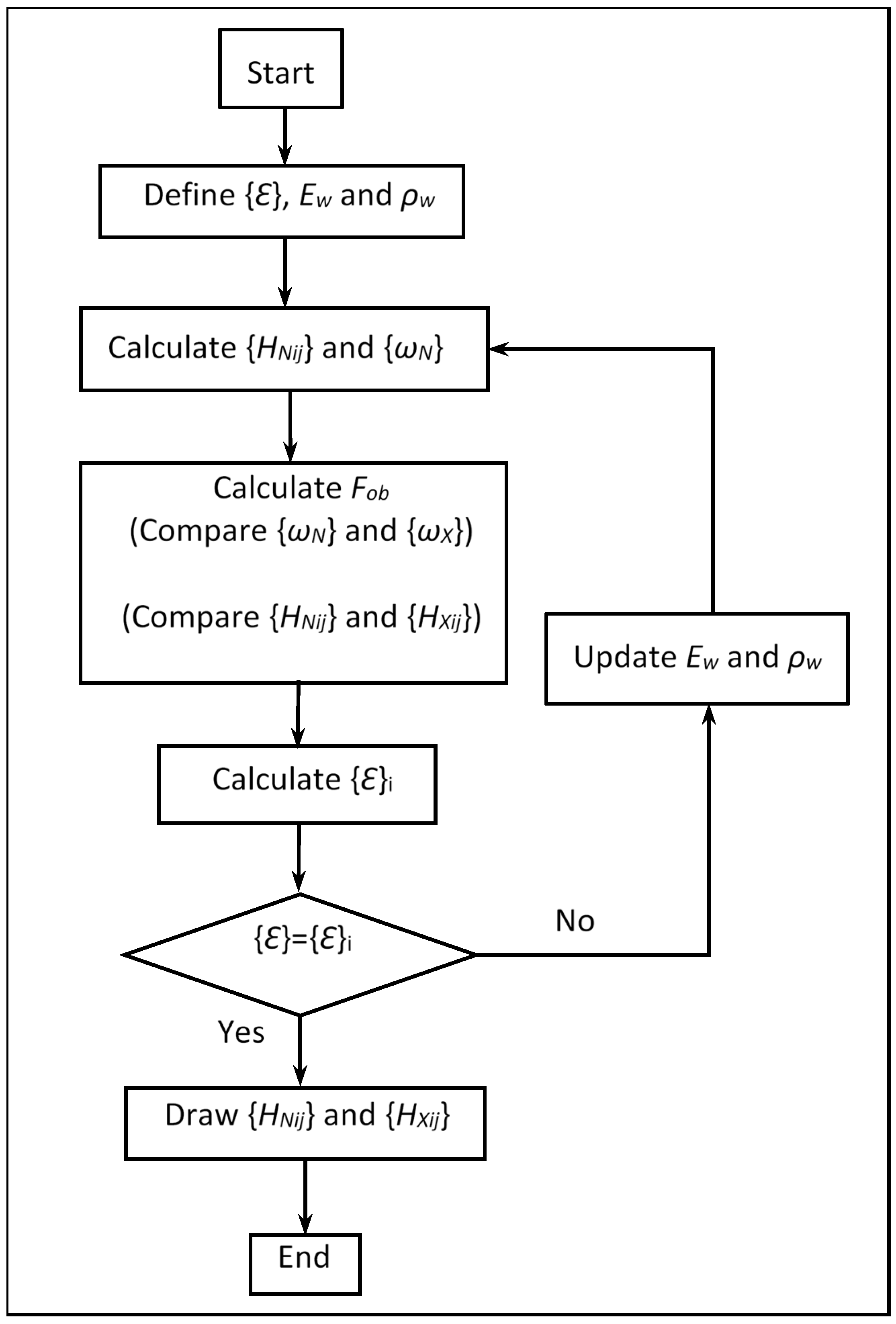
The values of the modulus of elasticity E_w and the mass density ρ_w of the friction weld zone are not known. The friction welding area was examined by cutting it in the longitudinal direction, and the ratio of the length of this region to the length of the combined beam was taken as 1/10. E_w and ρ_w were determined using a model updating procedure utilizing the dynamic properties of the friction-welded beams obtained with EMA. The model updating procedure is shown in Figure 8.

In friction welding processes, the weld zone exhibits variations in material structure due to the high temperatures generated and subsequent thermal diffusion. This typically leads to the formation of distinct regions: the heat-affected zone (HAZ), the thermomechanically affected zone (TMAZ), and the weld zone (WZ) itself. Depending on welding operational parameters such as rotational speed, forging force, or shortening, these regions subdivide into internal sub-regions, each displaying different mechanical properties. This variation arises from factors like stress concentrations and differences in grain size within these zones. In this study, the weld zone was analyzed as five distinct internal regions for each frequency value investigated. The updating process involved refining the elastic moduli and mass densities for each of these internal regions. Generally, a finer grain structure and a slight increase in material density are expected within the WZ due to the high temperatures. However, excessively high rotational speeds can sometimes lead to the opposite effect. Determining the optimum welding parameters requires detailed mechanical and microstructural examinations following operations conducted at various welding parameters. A similar situation applies to the TMAZ and HAZ. The thermal stresses developed in these regions are influenced by operational parameters, and this influence is often complex, making a straightforward analytical approach unrealistic. It is important to note that the model updating results presented in this study are specific to the welded beams investigated. Consequently, significantly different calculated updating parameters might be encountered for other structural geometries. Furthermore, the mechanical properties of the welded material, such as its mass density and elastic modulus, along with manufacturing tolerances of the materials, directly influence the model updating process.

In Figure 8, ε represents the convergence criterion. {H_Nij} and {H_Xij} are the numerical (calculated) and the experimental (measured) FRFs of the friction-welded beams, respectively. The subscript i denotes the response coordinate and j denotes the excitation coordinate of the corresponding FRF. Numerical and experimental FRFs, along with resonance frequencies, are employed in the model updating process for the joined beam. The objective is to approximate the point and transfer FRFs of the FE model to those of the experimental ones, thereby updating the numerical model by converging it towards the experimental model. The update parameters utilized are ρ_w and E_w of the weld zone. Here, ρ_w influences the mass matrix of the weld zone, while E_w affects the stiffness matrix and the initial values were taken as the values of the welded steel material SAE 304. These parameters are fed into the FRF similarity function, and the numerical and experimental FRFs are compared and updated through iterative adjustments of the update parameters.

For the FE model, the FRFs were calculated using Equation (13).

$${\alpha }_{\mathit{pq}}\left(\omega \right)={\displaystyle \sum _{r=1}^N\frac{{\varphi }_{\mathit{pr}}{\varphi }_{\mathit{qr}}}{\left(k_r-{\omega }^2{m}_r\right)+i{\eta }_r{k}_r}}$$

(13)

where ϕ_pr and ϕ_qr are the vibration mode shape elements of the rth mode shape for the coordinates p and q. The modal stiffness, modal mass, and modal damping ratio of the rth mode are expressed with k_r, m_r, and η_r, respectively, and ω is the frequency in rad/s.

FRF comparisons were made by using Equation (14) with FRAC (Frequency Response Assurance Criterion) for model updating.

$$\mathit{FRAC}={\displaystyle \frac{{\left|{\left\{H_{X_{\mathit{ij}}}(\omega )\right\}}^T\left\{H_{N_{\mathit{ij}}}(\omega )\right\}\right|}^2}{\left({\left\{H_{X_{\mathit{ij}}}(\omega )\right\}}^T\left\{H_{X_{\mathit{ij}}}(\omega )\right\}\right)\left({\left\{H_{N_{\mathit{ij}}}(\omega )\right\}}^T{\left\{H_{N_{\mathit{ij}}}(\omega )\right\}}^T\right)}}$$

(14)

In Figure 8, F_ob is the objective function as follows:

$$\begin{array}{l}{F}_{\mathit{ob}}(E_w,{\rho }_w)=a_1{\mathit{RMSE}}_N+a_2(1-\mathit{FRAC})\\ {\mathit{RMSE}}_N={\displaystyle \frac{\sqrt{\frac{1}{N}{\displaystyle {\sum }_{i=1}^N{\left|H_{X_{\mathit{ij}}}({\omega }_i)-H_{N_{\mathit{ij}}}({\omega }_i,E_w,{\rho }_w)\right|}^2}}}{\max \left(\left|H_{X_{\mathit{ij}}}\right|\right)}}\end{array}$$

(15)

where a₁ and a₂ are the weighting factors and RMSE_N is the normalized root mean square error.

3. Results and Discussion

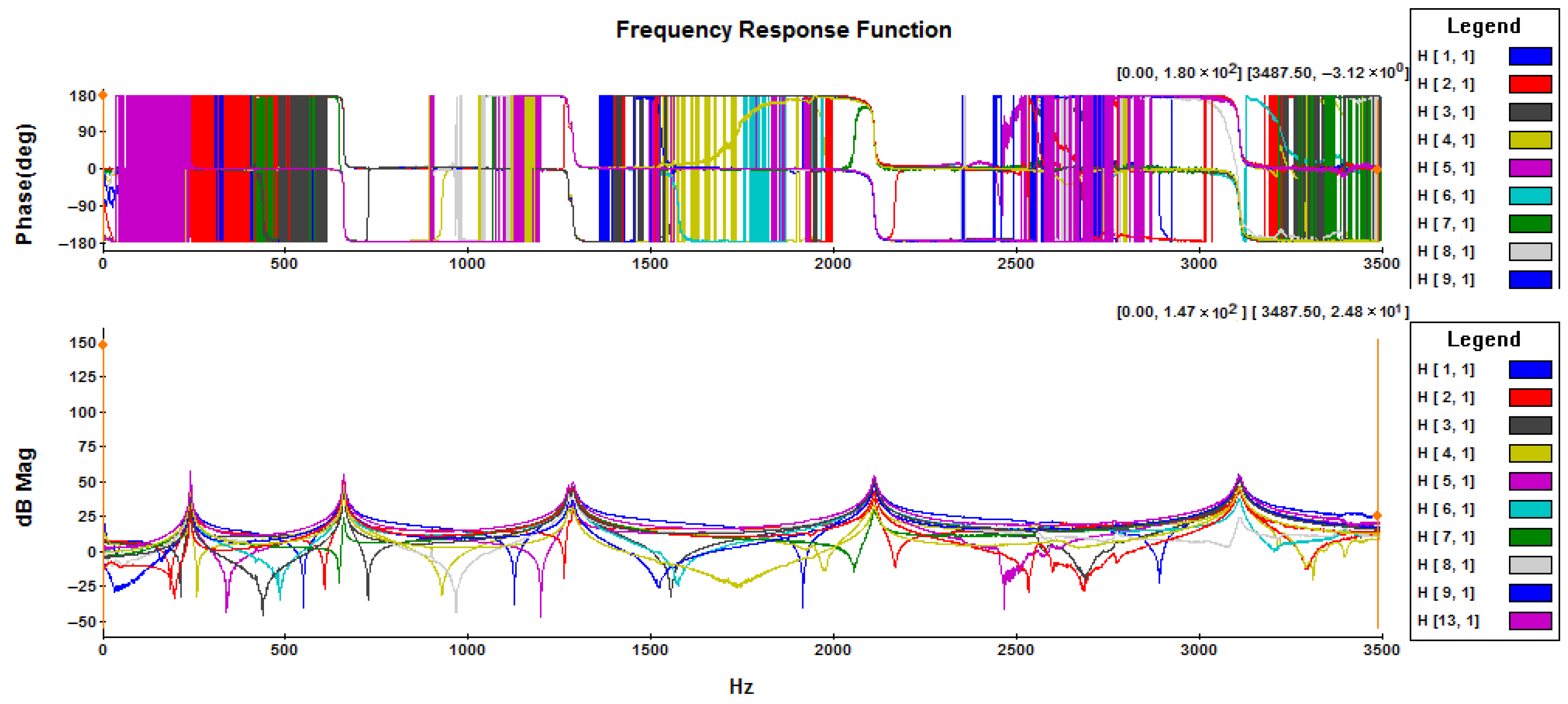
FRF graphs obtained with EMA are shown in Figure 9. The sharp peaks in Figure 9 indicate resonance frequencies and the reverse peaks indicate anti-resonance frequencies.

Resonance frequencies are global properties of a system and represent the poles of the system. Therefore, they appear in all FRFs of the system, as seen in Figure 9. Anti-resonance frequencies are local properties and represent the zeros of the system. Therefore, while they appear in some FRFs, they may not appear in others and may have different values.

The natural frequencies and damping ratios of the first five vibration modes obtained for each beam welded under different operation speeds are shown in

Table 1. Resonance frequencies of friction-welded beam under 1200 rpm operation speed.

1200 rpm	Resonance Frequencies (Hz)
	Mode 1		Mode 2		Mode 3		Mode 4		Mode 5
	Hz	Diff %	Hz	Diff %	Hz	Diff %	Hz	Diff %	Hz	Diff %
Experimental	240.5	-	660.4	-	1288.5	-	2112.8	-	3113.5	-
Reduced FEM	245.8	−2.2	677.7	−2.6	1329.0	−3.1	2198.4	−4.1	3288.6	−5.6
Updated FEM	234.2	−2.6	651.1	1.4	1269.2	1.5	2107.8	0.2	3147.5	−1.1

,

Table 2. Resonance frequencies of friction-welded beam under 1500 rpm operation speed.

1500 rpm	Resonance Frequencies (Hz)
	Mode 1		Mode 2		Mode 3		Mode 4		Mode 5
	Hz	Diff %	Hz	Diff %	Hz	Diff %	Hz	Diff %	Hz	Diff %
Experimental	240.2	-	659.6	-	1275.6	-	2109.9	-	3109.4	-
Reduced FEM	245.8	−2.3	677.7	−2.7	1329.0	−4.2	2198.9	−4.1	3289.6	−5.8
Updated FEM	237.0	2.2	650.5	1.3	1263.2	1.7	2103.1	0.4	3137.3	−0.8

and

Table 3. Resonance frequencies of friction-welded beam under 1800 rpm operation speed.

1800 rpm	Resonance Frequencies (Hz)
	Mode 1		Mode 2		Mode 3		Mode 4		Mode 5
	Hz	Diff %	Hz	Diff %	Hz	Diff %	Hz	Diff %	Hz	Diff %
Experimental	237.6	-	659.1	-	1283.0	-	2096.4	-	2990.9	-
Reduced FEM	245.8	−3.5	677.7	−2.8	1329.0	−3.6	2198.9	−4.9	3289.6	−9.9
Updated FEM	232.6	2.1	650.4	1.3	1261.3	1.7	2101.5	−0.2	3133.9	−4.8

.

The accuracy of the static model reduction method is expected to decrease in higher frequency ranges where inertia terms become more dominant. For the first five natural frequencies of bending vibrations investigated in this study, the difference between the experimentally obtained frequency values and those derived using the static model reduction method tends to progressively increase for higher modes, as anticipated. It is observed that this discrepancy significantly diminishes after model updating performed subsequent to static model reduction.

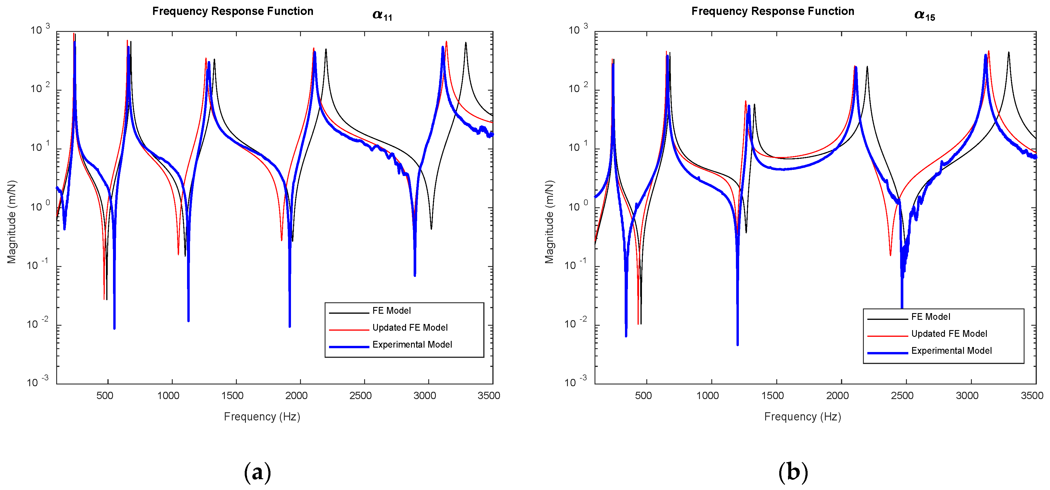
One of the FRF comparison graphs is given in Figure 10 including the FRFs of the experimental (blue line), reduced FE (black line), and the updated FE (red line) models. In Figure 10, it is seen that both in point and transfer FRFs, the presented FE model update method gives successful results.

The damping ratios for each obtained resonance frequencies were calculated and given for different welding operation speeds comparatively (Figure 11).

Vibration mode shapes for each resonance frequency for the specimens were obtained and are shown in Figure 12 below.

The vibration mode shapes of the friction-welded beams obtained using the EMA method were compared using the Modal Assurance Criterion (MAC) method to see the effects of operation parameters on vibration mode shapes using Equation (16).

$$MAC={\displaystyle \frac{{\left|{\left\{{\varphi }_A\right\}}_i^T{\left\{{\varphi }_B\right\}}_j\right|}^2}{\left({\left\{{\varphi }_B\right\}}_j^T{\left\{{\varphi }_B\right\}}_j\right)\left({\left\{{\varphi }_A\right\}}_i^T{\left\{{\varphi }_A\right\}}_i\right)}}$$

(16)

In Equation (16), ϕ_A and ϕ_B represent the mode shape vectors to be compared and (^T) is the transpose. The subscripts i and j in the equation represent the relevant mode. Accordingly, with a linear relationship between the two mode shape vectors examined, the MAC value will approach 1 and with no linear relationship, it will approach 0. In this way, the degree of the MAC value expresses the similarity rates of the mode shape vectors.

The vibration mode shapes given in Figure 12 were compared by calculating the MAC values and the similarities of the vibration mode shapes were determined (

Table 4. MAC values for friction-welded beams for 1500 rpm–1200 rpm.

1500 rpm	1200 rpm
	Frequencies (Hz)	240.5	660.4	1288.5	2112.8	3113.5	MAC Colors
	240.2	99.5	0.2	6.7	0.4	5.6
	659.6	0.1	99.7	0.2	7.2	0.1
	1275.6	6.0	0.1	99.3	0.2	3.9
	2109.9	0.2	7.7	0.1	99.4	0.1
	3109.4	6.3	0.1	6.3	0.1	98.5

,

Table 5. MAC values for friction-welded beams for 1500 rpm–1800 rpm.

1500 rpm	1800 rpm
	Frequencies (Hz)	237.6	659.1	1283.0	2096.4	2990.9	MAC Colors
	240.2	99.1	0.1	12.4	0.2	4.7
	659.6	0.0	99.9	0.1	9.5	0.0
	1275.6	6.6	0.0	97.9	0.0	13.8
	2109.9	0.1	7.3	0.0	99.6	0.2
	3109.4	7.1	0.1	5.6	0.1	96.3

and

Table 6. MAC values for friction-welded beams for 1200 rpm–1800 rpm.

1200 rpm	1800 rpm
	Frequencies (Hz)	237.6	659.1	1283.0	2096.4	2990.9	MAC Colors
	240.5	99.0	0.1	12.3	0.1	4.5
	660.4	0.1	99.8	0.1	10.2	0.0
	1288.5	7.2	0.0	97.5	0.1	14.6
	2112.8	0.2	7.3	0.2	99.4	0.3
	3113.5	5.9	0.1	3.8	0.1	93.8

).

According to the graphs given in Table 4, Table 5 and Table 6, from zero similarity to full similarity, the similarity relationship value increases from dark blue to red (full dark blue is 0, full red is 1). Here, 25 MAC values were calculated by examining five modes and proportional coloring was carried out for each similarity value obtained.

4. Conclusions

This paper deals with determining the vibration characteristics of rotational friction-welded beams produced under different welding operation speeds. The FE model of the friction-welded beam was created based on the Euler–Bernoulli beam approach using MATLAB and this FE model was reduced using the static model reduction method. The reduced FE model was then updated using the EMA test data. Some meaningful conclusions were obtained as follows:

• In EMA, the excitation and response coordinates consist of translational coordinates of nodal points defined on the beam. However, the numerical model includes both translational and rotational coordinates at the defined nodal points. To reduce the influence of rotational coordinates on the translational coordinates, a static model reduction technique was employed to condense the FE model. Since this study focuses on the frequency range encompassing the first five bending modes of the friction-welded specimens, the static reduction method was deemed suitable.
• Experimental Modal Analysis (EMA) was conducted for each specimen prepared under three distinct friction welding operation parameters (1200, 1500, and 1800 rpm) to determine their dynamic characteristics. Within this scope, resonance frequencies, corresponding damping ratios, and vibration mode shapes pertaining to the first five bending modes were ascertained. A slight decrease in resonance frequency values was observed with the transition from lower to higher rotational speeds. This phenomenon is hypothesized to stem from the finer grain structure of the material and increased mass density of the weld zone at higher rotational speeds. Additionally, it is postulated that the variation in rotational speeds during welding processes influences the modulus of elasticity of the weld zone, subsequently impacting the natural frequencies. The largest difference of 3.28% was observed in the first vibration mode and the smallest difference of 0.19% was observed in the second vibration mode.
• As a result of the analyses performed with EMA, vibration damping ratios corresponding to each resonance frequency were obtained. Accordingly, it was observed that the damping ratio increased significantly at the frequency corresponding to the third vibration mode of the sample obtained at low speed operation. Apart from this, the damping ratios tend to increase with increasing operation speed. The lowest vibration damping ratio belongs to the fourth mode at 1200 rpm with 0.119%.
• An algorithm utilizing the elastic modulus and mass density of the weld zone as updating parameters was developed for FE model updating. In the proposed algorithm, the discrepancies between the FRFs and resonance frequencies obtained from EMA and the FE model are minimized by calculating the necessary updating parameters. The FE model is then updated based on these calculated parameters to converge towards the experimental model. It was observed that the updated FE model closely approximates the experimental model, achieving an average of 2.30%, 1.33%, 1.63%, 0.26%, and 2.23% difference for the first five vibration modes, respectively.
• The vibration mode shapes of the specimens obtained at different operational speeds were computed and compared using Modal Assurance Criterion (MAC) graphs and tables. Examination of the mode shapes revealed a distinct chisel transition at the weld zone, particularly in the fourth and fifth vibration modes. However, analysis of the MAC graphs indicates that varying operational speeds do not significantly influence the mode shape similarities. In each comparison, the vibration mode shape similarities were found to be above 90%, with the highest similarity observed at 99.9% (second mode, 1500–1800 rpm) and the lowest at 93.8% (fifth mode, 1200–1800 rpm).

For future studies, researchers can investigate the dynamic analyses of structures fabricated by Rotary Friction Welding under various operational parameters. In this context, they can determine the dynamic characteristics of structures obtained by joining materials with different properties using friction welding. Furthermore, they can optimize rotational speeds to achieve specific dynamic properties by analyzing the changes in dynamic characteristics of welds made at different speeds within a broader range of rotational speeds. Additionally, they can explore the dynamic behaviors under different shortenings and pressures.

References

1. Marimuthu, S.; Balasubramanian, K.R.; Kannan, T.T.M. Mechanical and surface morphology study of Monel—Copper joint by rotary friction welding. Mater. Today Proc. 2021, 37, 419–424. [Google Scholar] [CrossRef]
2. Anandaraj, J.A.; Rajakumar, S.; Balasubramanian, V.; Petley, V. Investigation on mechanical and metallurgical properties of rotary friction welded In718/SS410 dissimilar materials. Mater. Today Proc. 2021, 45, 962–966. [Google Scholar] [CrossRef]
3. Singh, R.; Sharma, V. Molecular dynamics study of tensile behaviour for cold and linear friction welded single crystal tungsten. J. Mol. Graph. Model. 2020, 99, 107655. [Google Scholar] [CrossRef]
4. Orlowska, M.; Olejnik, L.; Campanella, D.; Buffa, G.; Morawinski, L.; Fratini, L.; Lewandowska, M. Application of linear friction welding for joining ultrafine grained aluminium. J. Manuf. Proc. 2020, 56, 540–549. [Google Scholar] [CrossRef]
5. Nicholas, E.D. Friction Processing Technologies. Weld. World 2003, 47, 2–9. [Google Scholar] [CrossRef]
6. Kimura, M.; Ohara, K.; Kusaka, M.; Kaizu, K.; Hayashida, K.J. Effects of tensile strength on friction welding condition and weld faying surface properties of friction welded joints between pure copper and austenitic stainless steel. J. Adv. Join. Process. 2020, 2, 100028. [Google Scholar] [CrossRef]
7. Balasubramanian, M.; Murali, S.; Hemadri, C.; Kumar, R. A new method of dissimilar friction welding of titanium to stainless steel. Mater. Today Proc. 2021, 46, 3644–3647. [Google Scholar] [CrossRef]
8. Vyas, H.D.; Mehta, K.P.; Badheka, V.; Doshi, B. Processing and evaluation of dissimilar Al-SS friction welding of pipe configuration: Nondestructive inspection, properties, and microstructure. Measurement 2021, 167, 108305. [Google Scholar] [CrossRef]
9. Albuquerque, A.A.; Louche, H.; Oliveira, D.F.; Brito, I.C.A. Rotary friction welding applied to Cu11.8Al0.45Be shape memory alloy. J. Adv. Join. Process. 2024, 10, 100233. [Google Scholar] [CrossRef]
10. Becheikh, N.; Tashkandi, M.A. Continuous Drive Friction Welding of Graphene-Reinforced AA6061 Alloy: Innovative Approach to Enhance Mechanical and Thermal Properties. J. Mater. Eng. Perform. 2024, 34, 6951–6962. [Google Scholar] [CrossRef]
11. Bouarroudj, E.; Chikh, S.; Abdi, S.; Miroud, D. Thermal analysis during a rotational friction welding. Appl. Therm. Eng. 2017, 110, 1543–1553. [Google Scholar] [CrossRef]
12. Jedrasiak, P.; Shercliff, H.R.; McAndrew, A.R.; Colegrove, P.A. Thermal modelling of linear friction welding. Mater. Des. 2018, 156, 362–369. [Google Scholar] [CrossRef]
13. Lei, B.; Shi, Q.; Yang, L.; Liu, C.; Pan, J.; Chen, G. Evolution of interfacial contact during low pressure rotary friction welding: A finite element analysis. J. Manuf. Process. 2020, 56, 643–646. [Google Scholar] [CrossRef]
14. Winiczenko, R.; Skibicki, A. Experimental and FEM Studies of Continuous Drive Friction Welding of Ferritic Spheroidal Graphite Cast Iron. Processes 2024, 12, 719. [Google Scholar] [CrossRef]
15. Wang, H.; Qin, G.; Fu, B.; Gao, Y.; Li, C. A novel method to establish friction coefficient model for numerical simulation of inertia friction welding. Mater. Des. 2024, 245, 113234. [Google Scholar] [CrossRef]
16. Nagasankar, P.; Gurusamy, P.; Gopinath, S.; Gnanaprakash, K.; Pradeep, G. Optimization of process parameters on engine exhaust valves using Taguchi method in friction welding process. Mater. Today Proc. 2020, 33, 3212–3217. [Google Scholar] [CrossRef]
17. Deepak Kumar, M.; Palani, P.K.; Karthik, V. Effect of welding parameters on joint strength of rotary friction welded UNS S31803 tubes. Mater. Today Proc. 2021, 39, 1265–1269. [Google Scholar] [CrossRef]
18. Jeong, H.S.; Cho, J.R.; Oh, J.S.; Kim, E.N.; Choi, S.G.; Ha, M.Y. Inertia Friction Welding Process Analysis and Mechanical Properties Evaluation of Large Rotor Shaft in Marine Turbo Charger. Int. J. Precis. Eng. Manuf. 2010, 11, 83–88. [Google Scholar] [CrossRef]
19. Gaikwad, V.T.; Balasundar, I.; Tripathi, A.; Singh, R.K.P.; Mishra, M.K. Microstructure evolution and mechanical properties of friction welded IN713LC and AISI 4140. Mater. Sci. Technol. 2024, 40, 909–920. [Google Scholar] [CrossRef]
20. Su, Y.; Li, W.; Wang, X.; Ma, T.; Yang, X.; Vairis, A. On microstructure and property differences in a linear friction welded nearalpha titanium alloy joint. J. Manuf. Process. 2018, 36, 255–263. [Google Scholar] [CrossRef]
21. Karadge, M.; Preuss, M.; Withers, P.J.; Bray, S. Importance of crystal orientation in linear friction joining of single crystal to polycrystalline nickel-based superalloys. Mater. Sci. Eng. A 2008, 491, 446–453. [Google Scholar] [CrossRef]
22. Reyes, A.E.S.; Rodriguez, G.A.L.; Parra, J.R.G.; Lemus, V.H.M. Microstructural Characterization and Corrosion Behavior of Similar and DissimilarWelded Advanced High-Strength Steels (AHSS) by Rotary Friction Welding. Materials 2024, 17, 918. [Google Scholar] [CrossRef] [PubMed]
23. Mani, H.; Taherizadeh, A.; Sadeghian, B.; Sadeghi, B.; Cavaliere, P. Thermal–Mechanical and Microstructural Simulation of Rotary FrictionWelding Processes by Using Finite Element Method. Materials 2024, 17, 815. [Google Scholar] [CrossRef] [PubMed]
24. Zhao, P.; Li, P.; Ding, Z.; Wang, J.; Zhang, C.; Zhao, Q.; Dong, H. Microstructural characterization and mechanical properties of inertia friction welded FGH96 joints. Mater. Today Commun. 2025, 42, 111194. [Google Scholar] [CrossRef]
25. Xu, X.; You, G.; Ding, Y.; Tong, X.; Zai, L.; Liu, Q. Microstructure and mechanical properties of inertia friction welded joint between high-strength low-alloy steel and medium carbon steel. J. Mater. Process. Technol. 2020, 286, 116811. [Google Scholar] [CrossRef]
26. Geng, P.; Qin, G.; Li, C.; Wang, H.; Zhou, J. Study on the importance of thermo-elastic effects in FE simulations of linear friction welding. J. Manuf. Process. 2020, 56, 602–615. [Google Scholar] [CrossRef]
27. Polami, S.M.; Reinhardt, R.; Rethmeier, D.; Schmid, A. Joint-site structure friction welding method as a tool for drive pinionlight weighting in heavy-duty trucks. J. Mater. Process. Technol. 2014, 214, 1921–1927. [Google Scholar] [CrossRef]
28. Buzzatti, D.T.; Buzzatti, J.T.; Lemos, G.V.B.; Amavisca, C.V.; Oliveira, D.L.P.; Mattei, F.; Dalpiaz, G.; Reguly, A. Towards friction welding to API grade B steel pipes. J. Adv. Join. Process. 2020, 2, 100026. [Google Scholar] [CrossRef]
29. Chen, J.C.; Wada, B.K. Criteria for analysis-test correlation of structural dynamic systems. J. Appl. Mech. 1975, 42, 471–477. [Google Scholar] [CrossRef]
30. Sidhu, J.; Ewins, D.J. Correlation of finite element and modal test studies of a practical structure. In Proceedings of the 2nd International Modal Analysis Conference, Orlando, FL, USA, 6–9 February 1984; Volume 2, pp. 756–762. [Google Scholar]
31. Gang, X.; Chai, S.; Allemang, R.J.; Li, L. A new iterative model updating method using incomplete frequency response function data. J. Sound Vib. 2014, 333, 2443–2453. [Google Scholar] [CrossRef]
32. Yuen, K.V.; Katafygiotis, L.S. Bayesian time-domain approach for modal updating using ambient data. Probabilistic Eng. Mech. 2001, 16, 219–231. [Google Scholar] [CrossRef]
33. Guyan, R.J. Reduction of stiffness and mass matrices. AIAA J. 1965, 3, 380. [Google Scholar] [CrossRef]
34. Rouch, K.E.; Kao, J.S. Dynamic reduction in rotor dynamics by the finite element method. J. Mech. Des. 1980, 102, 360–368. [Google Scholar] [CrossRef]
35. Tiwari, R. Rotor Systems: Analysis and Identification; CRC Press: Boca Raton, FL, USA, 2018. [Google Scholar]
Figure 1. Friction welding, (a) placement in machine, (b) alignment, (c) welding, (d) finishing.
Machines 13 00653 g001
Figure 2. Friction-welded beams.
Machines 13 00653 g002
Figure 3. Friction-welded beam prepared for Experimental Modal Analysis.
Machines 13 00653 g003
Figure 4. EMA test configuration.
Machines 13 00653 g004
Figure 5. EMA test setup: (a) test system, (b) measurement.
Machines 13 00653 g005
Figure 6. The coordinates of the beam element.
Machines 13 00653 g006
Figure 7. FE modeling of friction-welded beam.
Machines 13 00653 g007
Figure 8. The flow chart of the FE model updating procedure.
Machines 13 00653 g008
Figure 9. FRF graphs obtained from friction-welded beams.
Machines 13 00653 g009
Figure 10. FRF graphs obtained from friction-welded beams: (a) point FRF, (b) transfer FRF.
Machines 13 00653 g010
Figure 11. Comparisons for different welding parameters: (a) resonance frequencies, (b) damping ratios.
Machines 13 00653 g011
Figure 12. Vibration mode shapes of friction-welded beams under 1500 rpm welding operation speed.
Machines 13 00653 g012