Rolling Bearing Life Prediction Based on Improved Transformer Encoding Layer and Multi-Scale Convolution

Abstract

To accurately and reliably characterize the degradation trend of rolling bearings and predict their life cycle, this paper proposes a bearing life prediction model based on an improved transformer encoder layer and multi-scale convolution. First, time-domain, frequency-domain, and time-frequency domain features are extracted from the vibration data covering the entire lifespan of the rolling bearings and passed through the transformer encoder layer. A novel dual-layer self-attention mechanism network structure is proposed to capture global information on the lifecycle progression of rolling bearings. Next, to further extract local temporal features within the bearing’s life cycle, a multi-scale convolution module is proposed to reinforce the local information across the entire lifespan. This method fully exploits both the long-term trends and short-term dynamic variations in the health status of rolling bearings, effectively enhancing the accuracy of life predictions. Experimental results show that, even under conditions with interference features, the TransCN model outperforms mainstream advantage model in terms of prediction accuracy and generalizability. This approach offers a new solution for managing the fault risk of rotating machinery and reducing maintenance costs.

1. Introduction

Rolling bearings are mainly responsible for supporting rotating shafts and reducing friction [1] and play a vital role in ensuring the smooth and efficient operation of rotating machinery. However, high loads, insufficient lubrication, and contamination can lead to gradual degradation of bearings [2,3]. Once bearing failure occurs, it is easy to cause damage to the equipment, huge economic losses, and even casualties. Prognostics and Health Management (PHM) [4] techniques for predicting the Remaining Useful Life (RUL) of rolling bearings can reveal the deterioration process of the equipment, which can help to make reasonable maintenance decisions and reduce the safety risks of mechanical equipment [5]. It is also a key challenge and an important topic in the field of engineering [6,7,8].

The prediction methods of the Remaining Useful Life of rolling bearings are mainly divided into two categories: one is based on model-driven methods and the other is based on data-driven methods [4]. The model-driven method establishes a mathematical or physical model based on the failure mechanism of the bearing [9,10], which is not very generalizable due to the complexity of the actual working conditions and its randomness, and requires the use of personnel with a wealth of expert experience [11]. The data-driven approach mainly collects vibration data sets that characterize the health state of bearings and then obtains the complex nonlinear mapping relationship between the data sets and RUL by deep learning. Compared with the traditional model-driven methods, the data-driven approach is more flexible, can adapt to the nonlinear and complex patterns in the data, and can automatically learn complex feature representations from a large amount of data without human intervention [12]. Therefore, data-driven based methods have become the mainstream methods for bearing RUL prediction.

Convolutional Neural Networks (CNN) and Recurrent Neural Networks (RNN) and their variants have been widely used in bearing life prediction tasks [13,14,15,16] to improve the accuracy and reliability of bearing life estimation. However, traditional CNN and RNN can affect the accuracy of bearing life prediction due to their limitations, such as the gradient vanishing or gradient exposing problem of RNN, and the insufficient ability of CNN to capture long-term dependencies and insensitivity to temporal location. Temporal Convolutional Network (TCN) [17] can better solve the above problems.

In 2017 Vaswani A [18] proposed the transformer architecture, which overcomes the limitations of traditional deep networks in dealing with temporal data and focuses on the relationship between temporal data through the mechanism of self-attention, which is more advantageous in long sequence prediction tasks. Tang x et al. [19] combined with the time series information captured by the LSTM network and the self-attention mechanism of the transformer network, effectively solved the problem of information loss in the LSTM network and improved the prediction accuracy. Zhou Z et al. [20] used trigonometric and cumulative transformations to correct the monotonicity and trend of the input features and then used the transformer model to predict the RUL of the bearings. Wei Y et al. [21] proposed a conditional variational transformer architecture combining local feature learning and global context modeling for improving the prediction accuracy of the RUL of bearings. Deng L et al. [22] proposed a rolling bearing RUL prediction method based on the probabilistic prediction model DeepAR-transformer (D-former), which combines the autoregressive property of DeepAR and the effective feature extraction capability of the transformer to improve the processing capability of long-term series data. Zhang M et al. [23] proposed the WTE trans framework, which combines the weighted time embedding module and the shift window transformer to explicitly enhance the time correlation modeling and significantly improve the prediction accuracy of RUL. Although the above research results have achieved certain results, the dot product algorithm with self-attention may lack sensitivity to the local context, which limits its ability to capture the dynamic changes in the health status of rolling bearings locally [24].

In summary, this paper proposes a rolling bearing life prediction model (TransCN) that incorporates an improved transformer encoding layer and multi-scale convolution module. The model combines the advantages of both, in which the self-attention mechanism module captures the subtle interaction features through the global perspective and combines them with the local dependency features provided by the multi-scale convolution module, which enables the model to take more influencing factors into account in the task of bearing life prediction, thus improving the accuracy of the prediction. The contributions of this study can be summarized as follows:

• The dual-layer self-attention mechanism is proposed to improve the transformer encoding layer, and the self-iteration of the self-attention mechanism is formed by stacking the self-attention layer. The first-layer self-attention mechanism captures the basic feature during the bearing degradation process and grasps the overall trend of the life process. The secondary layer self-attention mechanism reprocesses the output of the first layer, intensifies key features, and suppresses noise interference, thereby capturing the potential fluctuations and complex dynamic changes during the bearing degradation process more accurately.
• A multi-scale convolution module was designed. Through two layers of the same convolution layers with different convolution kernel configurations, the information on different scales in the bearing degradation feature was extracted and fused. This is conducive to the model capturing the local information of the bearing at different operating stages more comprehensively, thereby reflecting the degradation state of the bearing more accurately and effectively improving the model’s ability to recognize complex degradation patterns.
• The high performance and robustness of the TransCN model were verified through experiments conducted in a data environment containing interference features. The experimental results show that even in the presence of many interference features, the TransCN model can still maintain high prediction accuracy and stable generalization ability. This provides a more reliable prediction tool for failure risk management and maintenance cost reduction in rotating machinery.

The main work of this paper is as follows: the first part summarizes and analyzes the problems existing in the field of bearing life prediction; the second part introduces the multi-domain feature extraction for rolling bearings; the third part describes the details of the composition of the TransCN network; the fourth part conducts experimental verification using the PHM2012 public data set and discusses the limitations of the model proposed in this paper; and the fifth part summarizes the proposed method and experimental results.

2. Rolling Bearing State Feature Extraction

2.1. Multi-Domain Feature Extraction

It is difficult to comprehensively characterize the complex dynamic changes in the degradation stage of rolling bearings with a single feature. In order to more accurately assess the health process of bearings, this paper extracts the degradation features from multiple domains such as the time domain, the frequency domain, and the time-frequency domain, respectively.

In this paper, 19 common time domain features are extracted, as shown in

Table 1. Time domain feature.

Feature	Formula
Average	$T_1={\displaystyle \frac{1}{n}}{\displaystyle \sum _{i=1}^n{x}_i}$
Absolute average	$T_2={\displaystyle \frac{1}{n}}{\displaystyle \sum _{i=1}^n|}{x}_i|$
Maximum	$T_3=\max (x_i)$
Minimum	$T_4=\min (x_i)$
Peak	$T_5=\max |x_i|$
Peak-to-Peak	$T_6=T_3-T_4$
Root mean square	$T_7=\sqrt{{\displaystyle \frac{1}{n}}{\displaystyle \sum _{i=1}^n{x}_i^2}}$
Root amplitude	$T_8={\left({\displaystyle \frac{1}{n}}{\displaystyle \sum _{i=1}^n\sqrt{\left|x_i\right|}}\right)}^2$
Variance	$T_9={\displaystyle \frac{1}{n-1}}{\displaystyle \sum _{i=1}^n{(x_i-T_1)}^2}$
Standard deviation	$T_{10}=\sqrt{T_9}$
Kurtosis	$T_{11}={\displaystyle \frac{1}{n}}{\displaystyle \sum _{i=1}^n{x}_i^4}$
Skewness	$T_{12}={\displaystyle \frac{1}{n}}{\displaystyle \sum _{i=1}^n{x}_i^3}$
Waveform index	$T_{13}={\displaystyle \frac{T_7}{T_2}}$
Peak index	$T_{14}={\displaystyle \frac{T_5}{T_7}}$
Impulse index	$T_{15}={\displaystyle \frac{T_5}{T_9}}$
Margin index	$T_{16}={\displaystyle \frac{T_5}{T_8}}$
Clearance factor	$T_{17}={\displaystyle \frac{T_5}{T_7^2}}$
Kurtosis factor	$T_{18}={\displaystyle \frac{T_{11}}{T_7^4}}$
Variation index	$T_{19}={\displaystyle \frac{T_{10}}{T_1}}$

, where $n$ is the total number of sampling points and $x_i$ is the observation value of the $i$th sampling.

To further quantify the complexity of the running state of the bearing [25], eight entropy features are extracted based on the time domain, which are log energy entropy, Renyi entropy, Tsallis entropy, Shannon entropy, approximate entropy, fuzzy entropy, sample entropy, and permutation entropy, and are recorded as $E_1~E_8$. The calculation formula is as follows:

For time series $Y=[y(1),y(2),\dots ,y(n)]$, the calculation formulas of log energy entropy, Renyi entropy, Tsallis entropy, and Shannon entropy are as follows:

$$E_1={\displaystyle \sum _{i=1}^n\log }(y_i^2)$$

(1)

$$E_2={\displaystyle \frac{1}{1-\alpha }}\log \left({\displaystyle \sum _{i=1}^n{P}_{y_i}^{\alpha }}\right),\alpha >0 \mathrm{and} \alpha \ne 1$$

(2)

$$E_3={\displaystyle \frac{1}{\alpha -1}}\left(1-{\displaystyle \sum _{i=1}^n{P}_{y_i}^{\alpha }}\right)$$

(3)

When $\alpha =1$, Renyi entropy is transformed into Shannon entropy. The simplified Shannon entropy calculation formula is as follows:

$$E_4=-{\displaystyle \sum _{i=1}^{n}P}(y_i){\log }_{2}P(y_i)$$

(4)

where $P(y_i)$ is the probability that the random variable $Y$ takes the $i$th value.

For a given time series $Y$, it can be constructed as $y_m(n)$ [26].

$$y_m(n)=\{y(n),y(n+1),\dots ,y(n+m-1)\}$$

(5)

$d_{nj}^m$ is defined as the distance between $y_m(n)$ and $y_m(j)$.

$$d_{nj}^m=\max (|y(n+k)-y(j-k)|),k=0,1,\dots ,m$$

(6)

$C_n^m$ is the probability that $d_{nj}^m$ is less than $r$ under a given similarity tolerance $r$, where $\theta$ is the Heaviside function and $m$ is the embedding dimension.

$$C_n^m(r)={\displaystyle \frac{{\displaystyle \sum _{j=1}^{N-m+1}\theta }(d_{nj}^m-r)}{N-m+1}}$$

(7)

The approximate entropy, fuzzy entropy, and sample entropy are as follows:

$$E_5={\displaystyle \frac{1}{N-m+1}}{\displaystyle \sum _{n=1}^{N-m+1}l}n{C}_n^m(r)$$

(8)

$$E_6={\displaystyle \frac{1}{N-m+1}}{\displaystyle \sum _{n=1}^{N-m+1}{C}_n^m}(r)$$

(9)

$$E_7={\displaystyle \frac{1}{N-m}}{\displaystyle \sum _{n=1}^{N-m}{C}_n^m}(r)$$

(10)

The $m$-dimensional vector $A$ can be constructed by reconstructing the phase space of a given time series $y(n)$.

$$A=\left[\begin{array}{cccc}{y}_{(1)}& y_{(1+\lambda )}& \dots & y_{(1+(m-1)\lambda )}\\ y_{(2)}& y_{(2+\lambda )}& \dots & y_{(2+(m-1)\lambda )}\\ ⋮& ⋮& \ddots & ⋮\\ y_{(\gamma )}& y_{(\gamma +\lambda )}& \dots & y_{(\gamma +(m-1)\lambda )}\end{array}\right]$$

(11)

where $\lambda$ is the delay time and $\gamma$ is the number of reconstructed components.

Sorting the $y$ in each reconstructed component in ascending order will lead to $m!$ different permutations. If the probability of occurrence of the $i$th arrangement is $P_i$, the arrangement entropy formula is as follows:

$$E_8^{\prime }=-{\displaystyle \sum _{i=1}^{\gamma }{P}_i}ln{P}_i$$

(12)

Finally, the permutation entropy is normalized.

$$0\le E_8={\displaystyle \frac{E_8^{\prime }}{\ln (m!)}}\le 1$$

(13)

Seven frequency domain features are extracted in this paper, as shown in

Table 2. Frequency domain features.

Feature	Formula
Mean Frequency	$F_1={\displaystyle \frac{1}{n}}{\displaystyle \sum _{i=1}^n{X}_i}$
Frequency standard	$F_2=\sqrt{{\displaystyle \frac{1}{n-1}}{\displaystyle \sum _{i=1}^n{(X_i-F_1)}^2}}$
Frequency center of gravity	$F_3={\displaystyle \frac{1}{n}}{\displaystyle \sum _{i=1}^n{f}_i}$
RMS Frequency	$F_4=\sqrt{{\displaystyle \frac{{\displaystyle \sum _{i=1}^n{f}_i^2}{X}_i}{{\displaystyle \sum _{i=1}^n{X}_i}}}}$
$F_5$	$F_5=\sqrt{{\displaystyle \frac{{\displaystyle \sum _{i=1}^n{(X_i-F_1)}^3}}{n\sqrt{F_4^3}}}}$
$F_6$	$F_6=\sqrt{{\displaystyle \frac{{\displaystyle \sum _{i=1}^n{(X_i-F_1)}^4}}{n{F}_4^2}}}$
$F_7$	$F_7=\sqrt{{\displaystyle \frac{{\displaystyle \sum _{i=1}^n{(f_i-F_3)}^2}{X}_i}{n}}}$

. Where $f_i$ is the signal frequency and $X_i$ is the spectrum amplitude.

Time frequency domain analysis combines the advantages of time domain and frequency domain analysis and can capture the changes in signal in time and frequency. In this paper, a three-layer wavelet packet decomposition is adopted to extract eight frequency band energy features of rolling bearings [27] which are recorded as $T{F}_1~T{F}_8$. The original signal can be recursively decomposed by the wavelet packet algorithm as follows.

$$x_{j+1,2k}(t)={\displaystyle \sum _{m}h}(m-2n)x_{j,k}(t)$$

(14)

$$x_{j+1,2k+1}(t)={\displaystyle \sum _{m}g}(m-2n)x_{j,k}(t)$$

(15)

$$g(n)={(-1)}^{n}h(1-n)$$

(16)

where $x_{j,k}(t)$ represents the wavelet coefficient of the $k$th subband in the $j$th layer.

Therefore, the original signal can be expressed as follows:

$$x(t)={\displaystyle \sum _{k=0}^{2^j-1}{x}_{j,k}}(t)$$

(17)

where $j$ and $k$ are the levels and subbands of wavelet packet decomposition, respectively.

2.2. Feature Normalization Processing

To eliminate the influence of each dimension of the feature, improve the convergence speed of the deep learning model, facilitate data analysis and processing, and avoid the problem of gradient exploring in the prediction process, this paper uses the max–min normalization method to map the extracted multi-domain feature set to the [0,1] interval. The calculation formula is as follows:

$$x^{*}={\displaystyle \frac{x-x_{\min }}{x_{\max }-x_{\min }}}$$

(18)

where $x_{\max }$ is the maximum value of the feature and $x_{\min }$ is the minimum value of the feature.

3. Rolling Bearing Life Prediction Based on Improved Transformer

3.1. Transformer Architecture

Transformer networks typically consist of an encoder and a decoder, where the encoder converts an input sequence into a continuous vector representation, and the decoder converts these representations into an output sequence. The self-attention layer introduces a multi-head attention mechanism to capture different subspace information, and each “head” independently learns different aspects of the data to obtain richer information expression and improve the training efficiency [28]. At the same time, location coding is used to make the model understand the sequence of each time point. In addition, the transformer uses residual connection and layer normalization after each sub-layer to help mitigate deep network gradient vanishing and stabilize the training process. The transformer performs well when handling complex sequential tasks, especially in scenarios such as rolling bearing life prediction that require long-distance dependencies and parallel processing [29]. To fully obtain the context dependence and characteristics of time series, make the model lighter and more efficient, and maintain good prediction accuracy, only the transformer encoder is used in this paper.

3.2. TransCN Model Structure

To take into account the global and local state features of rolling bearings, this paper proposes a TransCN model, which can not only capture the global trend in the process of bearing degradation but also sensitively identify the local information of the running state of rolling bearings, which can provide a more comprehensive and accurate rolling bearing life prediction solution. The model is mainly composed of the bottom-level network (self-attention mechanism module) and the top-level network (multi-scale convolutional module). The model structure is shown in Figure 1.

3.2.1. Bottom-Level Network

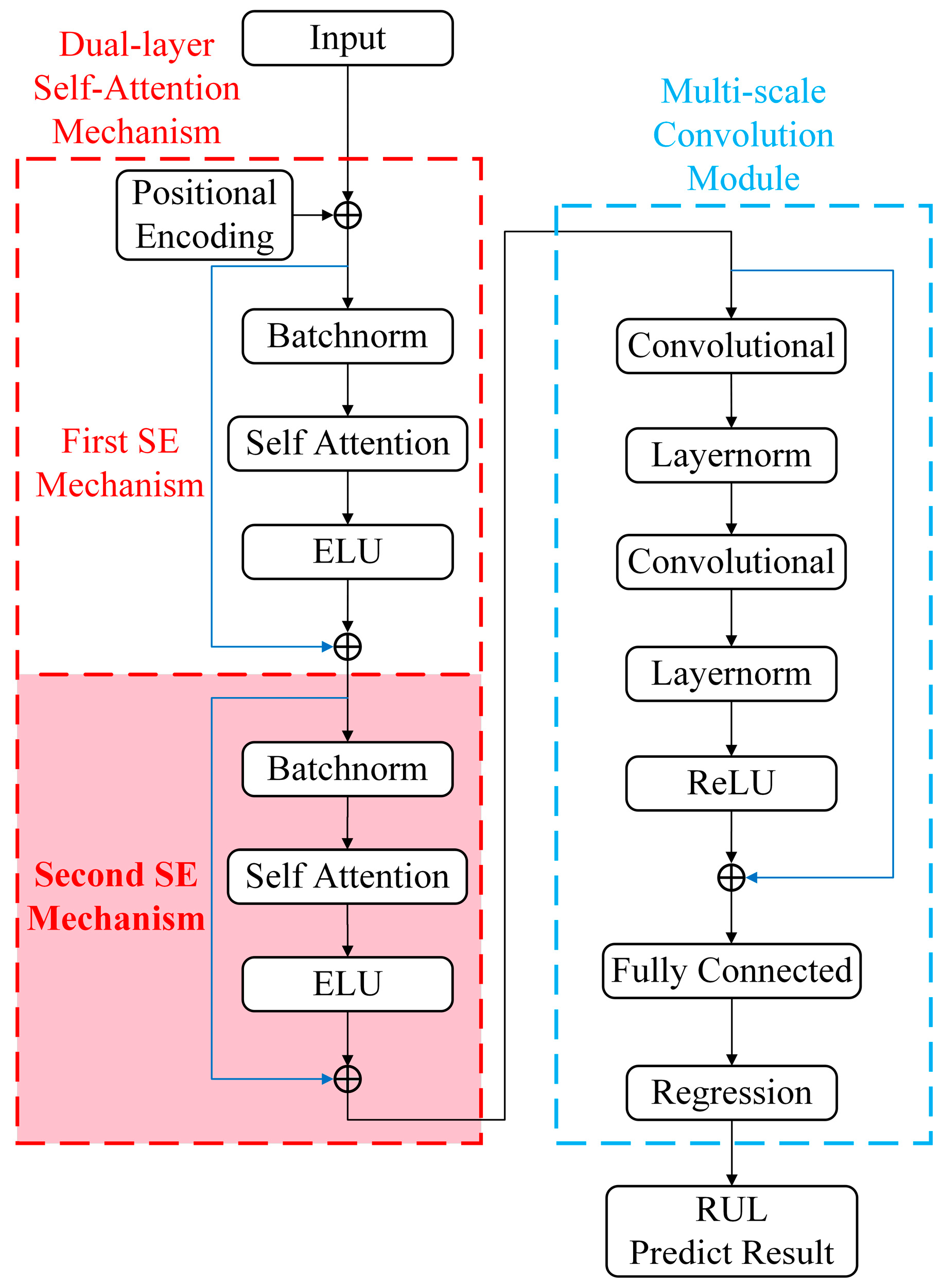
The proposed bottom-level network consists of the input layer, positional encoding layer, and self-attention mechanism module. (Figure 1 red dashed box)

• Input layer

This layer is responsible for accepting the multi-domain and multi-class feature sets of rolling bearing vibration, and the feature set comes from the bearing vibration signal information in the time domain, frequency domain, and time-frequency domain.

2.

Positional encoding layer

The positional encoding can save the time sequence for each time step; the calculation formula is as follows:

$$P{E}_{(pos,2i)}=\sin \left({\displaystyle \frac{pos}{{10000}^{\frac{2i}{d_{model}}}}}\right)$$

(19)

$$P{E}_{(pos,2i+1)}=\cos \left({\displaystyle \frac{pos}{{10000}^{\frac{2i}{d_{model}}}}}\right)$$

(20)

where $pos$ represents the position of the feature vector, $i$ represents the dimension of the positional encoding, and $d_{model}$ represents the dimension of the feature vector.

3.

Residual connection

Residual connections preserve the original input information and allow information to flow directly from the input layer to the subsequent layers, adding the input of one layer directly to the output of that layer. The output of the network can then be represented as a nonlinear transformation of the input and a linear superposition, that is, $y=F(x)+x$. This alleviates the problem of difficult information transfer in deep networks and helps maintain a more direct flow of information. This not only provides a direct propagation path for the gradient, alleviates the problem of gradient vanishing or exploding in deep network training, but also prevents the model from overfitting, enables the model to learn the general feature law, and enhances the generalization ability of new data. Residual connection is used in dual-layer self-attention mechanism and multi-scale convolution module in TransCN (as shown by the blue line in Figure 1).

4.

Attention mechanism module

The proposed attention mechanism module consists of batch normalization, self-attention mechanism, and ELU.

Self-attention connects two sequence positions to capture long-term dependencies in time series data. However, single-layer self-attention struggles to extract key degraded features from complex data. Thus, this study adds a second self-attention layer (pink shading in Figure 1) after the original in the transformer network. Batch normalization is applied to the input data to enhance model convergence and generalization, calculated as follows.

$$y_i=\gamma {\displaystyle \frac{x_i-\mu }{\sqrt{{\sigma }^2+\epsilon }}}+\beta$$

(21)

$${\sigma }^2={\displaystyle \frac{1}{B}}{\displaystyle \sum _{i=1}^B{(x_i-u)}^2}$$

(22)

$$\mu ={\displaystyle \frac{1}{B}}{\displaystyle \sum _{i=1}^B{x}_i}$$

(23)

where $x_i$ is the feature vector of the input and $\epsilon$ is a small value that prevents division by zero. The parameters $\gamma$ and $\beta$ are trainable.

The self-attention layer captures the global degradation trend of rolling bearing life from a global perspective, aiding the model in understanding bearing state evolution and providing critical information for life prediction. The formula is as follows:

The input feature matrix is $X$, and Query, Key, and Value matrices are generated by three sets of linear transformations.

$$Q=X{W}^Q$$

(24)

$$K=X{W}^K$$

(25)

$$V=X{W}^V$$

(26)

where $W^Q$, $W^K$ and $W^V$ are trainable parameter matrices.

Attention weights are calculated by the dot product of Query and Key:

$$Attention(Q,K,V)=Softmax\left({\displaystyle \frac{Q{K}^T}{\sqrt{d_k}}}\right)V$$

(27)

where $d_k$ is the dimension of $Q$ and $K$ matrices.

To capture attention for different features, a multi-head mechanism is used for parallel computation:

$$Multihead(Q,K,V)=Concat(hea{d}_1,hea{d}_2,\dots ,hea{d}_h)W^0$$

(28)

$$hea{d}_i=Attention\left(Q_i,K_i,V_i\right)$$

(29)

where $h$ is the number of attention heads, $W^o$ is the output transformation matrix. It should be noted that the algorithms of each self-attention in the proposed dual-layer self-attention mechanism are the same.

To introduce nonlinearity and enhance convergence, the self-attention output is activated by ELU. The formula is as follows:

$$ELU(x)=\left\{\begin{array}{cc}x,& x>0\\ \alpha (e^x-1),& x\le 0\end{array}\right.$$

(30)

where $\alpha$ is a hyperparameter which usually takes the value 1.

The dual-layer self-attention mechanism offers significant advantages. First, the first layer captures basic state evolution features of rolling bearings (trends and periods), while the second layer extracts deeper features (subtle changes and irregular patterns). This structure enables the model to handle more complex inputs. Secondly, the second layer refines the first layer’s output, enhancing focus on key fatigue features. For instance, in monitoring tasks, more accurately identifying fatigue features under different working conditions while suppressing less relevant noise. This targeted feature selecting enhances the model’s effectiveness in dynamic behavior modeling, improves adaptability, meets diverse data analysis needs, boosts generalization, and ensures robust performance in complex industrial environments.

3.2.2. Top-Level Network

The proposed top-level network includes a convolutional layer, layer normalization, ReLU, fully connected layer and a regressive layer. (Figure 1 blue dashed box)

• Convolutional layers

To take into account the local information of fatigue data of rolling bearings, this paper proposes that after the dual-layer self-attention mechanism, a one-dimensional same convolution layer with two layers of different convolution kerns is used to extract and merge the feature of bearing vibration signals at different scales to learn the complex nonlinear relationship between bearing vibration signals and their life course more effectively.

The one-dimensional same convolutional layer can flexibly control the receptive field by adjusting the size and step size of the convolution kernel while maintaining a low computational burden. Without increasing the difficulty of calculation, the design further introduces more nonlinearities by deepening the number of network layers to improve the expression ability of the model. In this paper, two same convolution layers can be used to further simplify the model structure and independently adjust the convolution kernel size and step size to adapt to different sequence lengths and feature extraction requirements, which helps to reduce the complexity of the model, reduce the risk of overfitting, and improve the generalization ability of the model, and extracting higher-level features layer by layer and fusion to improve the richness of feature expression. The model can capture and utilize the patterns in the data more effectively, which can further improve the accuracy of life prediction. The formula is as follows:

$$(f*g)(t)={\displaystyle {\int }_{-\infty }^{\infty }f}(\tau )g(t-\tau )d\tau$$

(31)

where $f(t)$ is the input signal, $g(t)$ is the convolution kernel, $*$ represents the convolution operation, $\tau$ is the integral variable used for the displacement in the convolution operation, and $(f*g)(t)$ is the result of the convolution operation, that is, the feature extracted by the convolution operation.

2.

Layer normalization

To reduce the influence of input distribution variation between layers, this paper performs layer normalization on input data to improve the training efficiency and stability of the model. Layer normalization utilizes the statistical information of a single sample and can maintain a stable gradient update effect when dealing with time series data. It is calculated as follows.

$$y_i=\gamma {\displaystyle \frac{x_i-\mu }{\sqrt{{\sigma }^2+\epsilon }}}+\beta$$

(32)

$${\sigma }^2=\frac{1}{B}\sum _{i=1}^B{(x_i-u)}^2$$

(33)

$$\mu =\frac{1}{B}\sum _{i=1}^B{x}_i$$

(34)

where $x_i$ is the feature vector of the input and $\epsilon$ is a small value that prevents division by zero. The parameters $\gamma$ and $\beta$ are trainable.

After normalization, the ReLU function is activated, and the life prediction value of the rolling bearing is obtained through the output of the regressive layer.

The primary purpose of the first convolution layer is to extract preliminary local features from the sequence. This layer is capable of capturing short-term patterns and trends in the sequence, and local features are crucial for understanding the real-time state of bearings, as they can reveal the dynamic changes in bearings at the microscopic level. The second convolution layer further refines the feature extraction process. This layer uses a different convolutional kernel configuration and is designed to capture more complex local features that are associated with a specific degradation pattern of the bearing. The introduction of the second convolutional layer enables the model to understand the bearing degradation process from a more fine-grained perspective, thereby enhancing the model’s ability to identify subtle changes in the bearing degradation process. By convolving the two layers in series, the model can capture local features on multiple scales, thereby providing a more comprehensive understanding of the bearing degradation process. This multi-scale feature extraction method helps the model capture the dynamic changes in bearings on different time scales, thus improving the accuracy and robustness of the prediction. The concatenation of two layers of convolution not only enhances the expression ability of the feature but also improves the recognition ability of complex degenerated patterns through the fusion of features at different scales. To stabilize the training process and accelerate convergence, after each convolution operation, layer normalization is added. Layer normalization reduces internal covariate offsets by normalizing feature values for each sample, which helps prevent gradient vanishing or exposing problems, thus making deep network training more stable. Therefore, the model can adapt to the distribution change in data faster, thereby improving the training efficiency and model performance. Finally, the ReLU activation function is used to introduce nonlinearity, which enables the model to identify and use the nonlinearity feature in the data to more accurately simulate the complex process of bearing degradation.

In summary, the life prediction model of rolling bearing proposed in this paper mainly has the following steps:

Step 1: the vibration signals of multiple bearings in the whole life cycle are collected, and the different bearings are divided into the training set and a test set.

Step 2: extract the multi-domain feature of the vibration signal, normalize the set of multi-domain features, and label it with a lifetime (Equations (18) and (35)).

Step 3: Build a dual-layer self-attention mechanism transformer encoding layer (Equations (24)–(29)). The first layer of attention captures the basic feature of the rolling bearing state, and the series structure of the second layer of attention forms the self-iteration of the attention mechanism to further extract the feature of the depth state.

Step 4: Construct the multi-scale convolution module (Equation (31)). The local feature of rolling bearing vibration signals in different time scales is extracted and fused.

Step 5: the output results of the model are smoothed (Equation (36)) to obtain the life prediction results.

As shown in Figure 2, the self-attention mechanism of the bottom-level network in the proposed model enables the model to identify and exploit long-term trends in the time series. Through the serial connection of self-attention mechanism, the feature is gradually extracted from the model at different abstraction levels. These features contain the global information of time series, providing a more comprehensive representation of time features for the proposed model, and laying a high-quality data foundation for further processing of subsequent top-level network. The top-level network uses the multi-scale convolution module to capture and fuse local features on different time scales, which enhances the sensitivity of the proposed model to regional changes in time series. Through convolution operation, the model can further refine and enhance the features transmitted from the bottom-level network, making the feature expression more abundant and accurate. By using this kind of division and cooperation mode of the top and bottom-level network series structure, the model can predict the life of the rolling bearing by using the global and local features at the same time and enhance the understanding ability of the model to the information of the bearing life process.

4. Experimental Verification

4.1. Data Set Description

To verify the effectiveness of the proposed method, this paper uses the IEEE PHM 2012 public data set for testing [30]. The PRONOSTIA experimental platform is equipped with two DYTRAN 3035B (Dytran by HBK, Chatsworth, CA, USA) micro-accelerometers, which are mounted on the outer ring of the rolling bearing in a radial way at 90° to each other. The two accelerometers collect the bearing vibration signal at a sampling frequency of 25.6 kHz, and the sampling is carried out every 10 s and the data are collected for 0.1 s each time. Figure 3 shows the testbed as well as the sensor arrangement.

This data set contains full-life vibration data of 17 bearings under three operating conditions. The specific operating conditions are shown in

Table 3. Bearing operating conditions.

Operating Conditions	Rotational Speed/rpm	Radial Force/kN	Bearing Number
1	1800	4.0	Bearing1_1~Bearing1_7
2	1650	4.2	Bearing2_1~Bearing2_7
3	1500	5.0	Bearing3_1~Bearing3_3

. In this paper, the data of working conditions 1 and 2 are selected to verify the model. In working condition 1, Bearing1_3 and Bearing1_7 are selected as the training set, and Bearing1_4 is selected as the test set. In condition 2, Bearing2_7 is selected as the training set and Bearing2_4 as the test set. In this paper, the horizontal vibration signal is selected for analysis.

The label of each sample Is defined as: current running time/total running time, distributed between 0 and 1, where 0 indicates that the bearing is completely healthy and 1 indicates that the bearing is completely damaged.

$$y_i={\displaystyle \frac{t_i}{T_e}}$$

(35)

where $t_i$ is the current time, $T_e$ is the failure time, and $y_i$ is the sample label at the current time.

4.2. Experiment 1

The features of Bearing1_3 and Bearing1_7 horizontal vibration signals in the time domain, frequency domain, and time-frequency domain are extracted for network training. The horizontal vibration signals and features of Bearing1_3 and Bearing1_7 are shown in Figure 4, Figure 5, Figure 6, Figure 7, Figure 8, Figure 9, Figure 10, Figure 11, Figure 12 and Figure 13. It can be seen that most features tend to be strong, such as T2–T10, E4, E6, F1, F2, F7, and TF4 of Bearing1_3 and T2–T11, T13, E2, E3, E6, E8, F1, F2, and F7 of Bearing1_7. To test the effectiveness, robustness and generalization of the proposed algorithm, no denoising operation was carried out on the original signal in this paper, and some features with poor quality were also included as strong interference items in the test data (as shown by the red label in Figure 6, Figure 7, Figure 8, Figure 9, Figure 10, Figure 11, Figure 12 and Figure 13). For example, Bearing1_3’s T14–T16, E1–E3, F3–F6, TF2, and TF5–TF8 and Bearing1_7’s T12, T14–T16, E1, TF1–TF3, TF5, and TF6 have very large burrs. T1 and T19 of Bearing1_3 and T1, T19, F3, F5, and F6 of Bearing1_7 do not change much during the whole life stage and do not reflect any information of bearing degradation.

The multi-domain feature set of Bearing1_3 and Bearing1_7 is input into the network for training. After the network is trained, the multi-domain feature set of Bearing1_4 is input into the network to predict the bearing life. MAE and MSE are selected as the error indexes of the life prediction results. The network hyperparameter Settings are shown in

Table 4. Experiment 1 hyperparameter setting.

Hyperparameters	Value
Epochs	50
BatchSize	100
Learning rate	0.00098
Multi-head attention head count	4
Size of the convolution kernel	4/5
The number of convolution kernels	42/42
Optimizer	Adam

.

To reduce the local oscillation of the predicted value, the moving average algorithm is used to smooth the life prediction results, so that the prediction results are more in line with the actual situation [14]. In this case, the window length is chosen to be 140, and the smoothing algorithm formula is as follows:

$$y_t=\{\begin{array}{ll}\frac{1}{\mathit{win}}{\displaystyle \sum _{i=1}^t}{x}_i,& t<\mathit{win}\\ \frac{1}{\mathit{win}}{\displaystyle \sum _{i=t-\mathit{win}+1}^t}{x}_i,& \mathit{win}\le t\le n-\mathit{win}+1\\ \frac{1}{\mathit{win}}{\displaystyle \sum _{i=1}^t}{x}_i,& t>n-\mathit{win}+1\end{array}$$

(36)

where $x_i$ is the original series and $y_t$ is the series after the moving average and the window size of $win$ moving average. The results of the lifetime prediction are shown in Figure 14.

According to Figure 14, fitting at the end of the full life of the rolling bearing shows that the proposed method predicts the bearing failure only 50 s in advance, accounting for 0.35% of the full life cycle of the bearing, which shows that the proposed model can accurately predict the bearing life. The error index of the life prediction result is MAE: 0.0767, MSE: 0.0090. On the whole, the life prediction result is basically consistent with the real life trend which reflects the degradation process of the bearing well.

To verify the effectiveness and generalization of the proposed model, this paper uses four current mainstream bearing life prediction models for comparison, as shown in Figure 15. The transformer encoder (blue curve) uses the self-attention mechanism to capture the global dependence and predicts the bearing degradation trend as a whole. However, the transformer encoder has relatively large errors in the early stage (before 1100 s) and poor compatibility with real life in the later stage (after 13,300 s), and predicts bearing failure 500 s in advance. It accounts for 3.50% of the whole life cycle of the bearing, and the error is large. Although TCN (light green curve) has advantages in capturing local features, it has shortcomings in extracting global features and predicting the overall trend. The prediction curve shows certain volatility, especially in the middle and late life (after 11,530 s), and there is a large deviation from the real life. Combining the advantages of the two methods, the proposed method is more comprehensive in feature extraction, and can better understand the complex dynamic changes in bearing degradation. The error metrics are shown in

Table 5. Experiment 1 error index of multi model prediction results.

Model	MAE	MSE
Method of this paper	0.0767	0.0090
CNN	0.1045	0.0126
GRU	0.1246	0.0184
TCN	0.1283	0.0258
Transformer Encoder	0.0964	0.0150

. Compared with CNN, GRU, TCN and transformer encoder, the MAE of the proposed method is reduced by 26.65%, 38.50%, 40.27% and 32.73%, and the MSE is reduced by 28.64%, 51.14%, 65.16% and 68.46%, respectively. It can be seen that the proposed method is superior to other methods.

4.3. Experiment 2

To further verify the generalization of the proposed model, under the same conditions, a feature of Bearing2_7 horizontal vibration signal in the time domain, frequency domain and time-frequency domain are extracted for network training. Bearing2_7 horizontal vibration signal and feature are shown in Figure 16, Figure 17, Figure 18, Figure 19 and Figure 20. It can be seen that most features show a certain overall growth or decline trend on the time axis, which is conducive to the life prediction of bearings, such as T2–T10, T17, T18, E4–E8, F1, F2, F4–F7, and TF1–TF4. At the same time, some features cannot reflect the degradation process of bearings (as shown in the red label in Figure 17, Figure 18, Figure 19 and Figure 20), such as T13–T16, E1–E3 and F3, there are very large fluctuations, T1, T11, T12 and T19 change steadily throughout the life stage, which does not help predict the degradation state of bearings. The bad features are input into the model as interference items for training, to verify the robustness of the model.

Bearing2_7’s multi-domain feature set is input into the network for training. After the network training is complete, Bearing2_4’s multi-domain feature set is input into the network to predict the bearing life. The network hyperparameter Settings are shown in

Table 6. Experiment 2 hyperparameter setting.

Hyperparameters	Value
Epochs	100
BatchSize	16
Learning rate	0.00395
Multi-head attention head count	4
Size of the convolution kernel	5/4
The number of convolution kernels	42/42
Optimizer	Adam

. The life prediction results are smoothed, in this case, the window length is chosen to be 40, and the life prediction results are shown in Figure 21.

The error index of life prediction results is MAE: 0.0618, MSE: 0.0065. It can be seen that the fitting effect of life prediction is very good, which well reflects the degradation trend of bearings. At the end of the bearing life, the bearing failure is only warned 50 s in advance, accounting for 0.67% of the whole life cycle of the bearing, which accurately predicts the failure of the bearing.

CNN, GRU, TCN, and transformer encoder models are used to compare with the prediction effect of this model, and the comparison effect is shown in Figure 22. It can be seen that although the transformer encoder (blue curve) captures the long-term dependence of the data and predicts the degradation trend well, the prediction accuracy is far from real life, and the prediction curve once seriously deviated from real life. Although TCN (light green curve) is good at capturing local features, it cannot extract global features, so the prediction effect is not ideal. The method in this paper combines the advantages of both and accurately predicts the bearing life. The error metrics are shown in

Table 7. Experiment 2 error index of multi model prediction results.

Model	MAE	MSE
Method of this paper	0.0618	0.0065
CNN	0.1367	0.0234
GRU	0.1682	0.0366
TCN	0.2450	0.0832
Transformer encoder	0.1140	0.0285

. Compared with CNN, GRU, TCN, and transformer encoder, the MAE of the proposed method is reduced by 54.79%, 63.26%, 74.44%, and 45.75%, and the MSE is reduced by 72.22%, 82.22%, 92.18%, and 77.18%, respectively. It can be seen that the proposed method is superior to other methods.

Combining the life prediction results of working conditions 1 and 2, the life prediction method proposed in this paper can dig out the nonlinear relationship between vibration signals and bearing life and can better predict the life process of rolling bearings.

In summary, the algorithm proposed in this paper is experimentally verified to achieve better performance, accuracy, and generalization of life prediction than many mainstream methods. It provides an effective solution for failure risk management of rotating machinery. We note that in real industrial scenarios, the speed and load of rolling bearings may face random dynamic changes. Such changing conditions may lead to fluctuations in vibration signal features. As a further direction of exploration, the study can consider introducing a dynamic feature extraction module and an online updating strategy to enhance the model’s adaptability to variable working conditions and extend the application scope of this study.

5. Conclusions

To further improve the accurate description of the rolling bearing degradation trend and life process, a TransCN model is proposed in this paper. By improving the encoding layer of the transformer and integrating it with the multi-scale convolution module, the accuracy of rolling bearing life prediction is effectively improved, and the following conclusions are drawn:

(1)

A new dual-layer self-attention mechanism is proposed to improve the transformer encoding layer to obtain the global features of rolling bearing time series. Through the concatenation of self-attention mechanism, the long-term trend of the time series can be effectively captured, and complex global dependencies and dynamic patterns can be modeled, providing a more comprehensive time representation for the model.

(2)

A two-layer same convolutional module structure is designed to capture local features of different scales in the fatigue evolution of rolling bearings and integrate them, which enhances the local feature extraction capability of the model, improves the computing efficiency of the model, and reduces the computing resource requirements.

(3)

The tests under different working conditions show that the life prediction results of TransCN fit the actual life curve, and the end of the bearing life is in good agreement, which proves that the model has a certain generalization ability. Compared with the mainstream life prediction model, the life error index is generally reduced by more than 45%. The results of this paper can provide a more accurate theoretical basis for the operation and maintenance of rotating machinery equipment.

References

1. Huang, G.; Lei, W.; Dong, X.; Zou, D.; Chen, S.; Dong, X. Stage-Based Remaining Useful Life Prediction for Bearings Using GNN and Correlation-Driven Feature Extraction. Machines 2025, 13, 43. [Google Scholar] [CrossRef]
2. He, M.; Li, Z.; Hu, F. A Novel RUL-Centric Data Augmentation Method for Predicting the Remaining Useful Life of Bearings. Machines 2024, 12, 766. [Google Scholar] [CrossRef]
3. Chen, B.; Smith, W.A.; Cheng, Y.; Gu, F.; Chu, F.; Zhang, W.; Ball, A.D. Probability distributions and typical sparsity measures of Hilbert transform-based generalized envelopes and their application to machine condition monitoring. Mech. Syst. Signal Process. 2025, 224, 112026. [Google Scholar] [CrossRef]
4. Cai, S.; Zhang, J.; Li, C.; He, Z.; Wang, Z. A RUL prediction method of rolling bearings based on degradation detection and deep BiLSTM. Electron. Res. Arch. 2024, 32, 3145–3161. [Google Scholar] [CrossRef]
5. Fan, Z.; Li, W.; Chang, K.C. A bidirectional long short-term memory autoencoder transformer for remaining useful life estimation. Mathematics 2023, 11, 4972. [Google Scholar] [CrossRef]
6. Ferreira, C.; Gonçalves, G. Remaining Useful Life prediction and challenges: A literature review on the use of Machine Learning Methods. J. Manuf. Syst. 2022, 63, 550–562. [Google Scholar] [CrossRef]
7. Lei, Y.; Li, N.; Guo, L.; Li, N.; Yan, T.; Lin, J. Machinery health prognostics: A systematic review from data acquisition to RUL prediction. Mech. Syst. Signal Process. 2018, 104, 799–834. [Google Scholar] [CrossRef]
8. Chen, B.; Cheng, Y.; Allen, P.; Wang, S.; Gu, F.; Zhang, W.; Ball, A.D. A product envelope spectrum generated from spectral correlation/coherence for railway axle-box bearing fault diagnosis. Mech. Syst. Signal Process. 2025, 225, 112262. [Google Scholar] [CrossRef]
9. Lei, Y.; Li, N.; Gontarz, S.; Lin, J.; Radkowski, S.; Dybala, J. A model-based method for remaining useful life prediction of machinery. IEEE Trans. Reliab. 2016, 65, 1314–1326. [Google Scholar] [CrossRef]
10. Tian, Z.; Liao, H. Condition based maintenance optimization for multi-component systems using proportional hazards model. Reliab. Eng. Syst. Saf. 2011, 96, 581–589. [Google Scholar] [CrossRef]
11. Singleton, R.K.; Strangas, E.G.; Aviyente, S. Extended Kalman filtering for remaining-useful-life estimation of bearings. IEEE Trans. Ind. Electron. 2014, 62, 1781–1790. [Google Scholar] [CrossRef]
12. Zhu, J.; Chen, N.; Shen, C. A new data-driven transferable remaining useful life prediction approach for bearing under different working conditions. Mech. Syst. Signal Process. 2020, 139, 106602. [Google Scholar] [CrossRef]
13. Guo, R.; Li, H.; Huang, C. Operation stage division and RUL prediction of bearings based on 1DCNN-ON-LSTM. Meas. Sci. Technol. 2023, 35, 025035. [Google Scholar] [CrossRef]
14. Yang, L.; Jiang, Y.; Zeng, K.; Peng, T. Rolling Bearing Remaining Useful Life Prediction Based on CNN-VAE-MBiLSTM. Sensors 2024, 24, 2992. [Google Scholar] [CrossRef] [PubMed]
15. Ma, P.; Li, G.; Zhang, H.; Wang, C.; Li, X. Prediction of remaining useful life of rolling bearings based on multiscale efficient channel attention CNN and bidirectional GRU. IEEE Trans. Instrum. Meas. 2024, 73, 1–13. [Google Scholar] [CrossRef]
16. Wen, L.; Su, S.; Li, X.; Ding, W.; Feng, K. GRU-AE-wiener: A generative adversarial network assisted hybrid gated recurrent unit with Wiener model for bearing remaining useful life estimation. Mech. Syst. Signal Process. 2024, 220, 111663. [Google Scholar] [CrossRef]
17. Lea, C.; Vidal, R.; Reiter, A.; Hager, G.D. Temporal convolutional networks: A unified approach to action segmentation. In Proceedings of the Computer Vision–ECCV 2016 Workshops, Amsterdam, The Netherlands, 8–10 and 15–16 Octorber 2016; Proceedings, Part III. Springer International Publishing: Berlin/Heidelberg, Germany, 2016; pp. 47–54. [Google Scholar]
18. Vaswani, A. Attention is all you need. In Proceedings of the Advances in Neural Information Processing Systems, Long Beach, CA, USA, 4–9 December 2017. [Google Scholar]
19. Tang, X.; Xi, H.; Chen, Q.; Lin, T.R. Rolling bearing remaining useful life prediction based on LSTM-Transformer algorithm. In Proceedings of IncoME-VI and TEPEN 2021: Performance Engineering and Maintenance Engineering; Springer International Publishing: Cham, Switzerland, 2022; pp. 207–215. [Google Scholar]
20. Zhou, Z.; Liu, L.; Song, X.; Chen, K. Remaining useful life prediction method of rolling bearing based on Transformer model. J. Beijing Univ. Aeronaut. Astronaut. 2021, 49, 430–443. [Google Scholar]
21. Wei, Y.; Wu, D. Conditional variational transformer for bearing remaining useful life prediction. Adv. Eng. Inform. 2024, 59, 102247. [Google Scholar] [CrossRef]
22. Deng, L.; Li, W.; Zhang, W. Intelligent prediction of rolling bearing remaining useful life based on probabilistic DeepAR-Transformer model. Meas. Sci. Technol. 2023, 35, 015107. [Google Scholar] [CrossRef]
23. Zhang, M.; He, C.; Huang, C.; Yang, J. A weighted time embedding transformer network for remaining useful life prediction of rolling bearing. Reliab. Eng. Syst. Saf. 2024, 251, 110399. [Google Scholar] [CrossRef]
24. Li, S.; Jin, X.; Xuan, Y.; Zhou, X.; Chen, W.; Wang, Y.-X.; Yan, X. Enhancing the locality and breaking the memory bottleneck of transformer on time series forecasting. Adv. Neural Inf. Process. Syst. 2019, 32, 5243–5253. [Google Scholar]
25. Xu, X.; Zhou, J.; Weng, X.; Zhang, Z.; He, H.; Steyskal, F.; Brunauer, G. A novel evidence reasoning-based rul prediction method integrating uncertainty information. Reliab. Eng. Syst. Saf. 2024, 250, 110250. [Google Scholar] [CrossRef]
26. Ke, Z.; Lin, B. Nonlinear characteristic measure of gearbox faults and their category identification with TWSVM. J. Vib. Shock. 2018, 37, 179–184. [Google Scholar]
27. Liu, X.; Luan, X.; Zhao, J.; Xiao, B.; Sha, Y. Aircraft engine rolling bearings based on comprehensive dynamic screening Fault feature extraction method. J. Aerosp. Power 2024, 40, 20240210-1–20240210-12. [Google Scholar]
28. Zhan, H.; Li, H.; Xiao, X. Prediction of Remaining Useful Life of Rolling Bearings based on Transformer Encoder. In Proceedings of the 2023 IEEE 7th Information Technology and Mechatronics Engineering Conference (ITOEC), Chongqing, China, 15–17 September 2023; Volume 7, pp. 355–359. [Google Scholar]
29. Li, X.; Li, J.; Zuo, L.; Zhu, L.; Shen, H.T. Domain adaptive remaining useful life prediction with transformer. IEEE Trans. Instrum. Meas. 2022, 71, 1–13. [Google Scholar] [CrossRef]
30. Nectoux, P.; Gouriveau, R.; Medjaher, K.; Ramasso, E.; Morello, B.; Zerhouni, N.; Varnier, C. PRONOSTIA: An experimental platform for bearings accelerated degradation tests. In Proceedings of the IEEE International Conference on Prognostics and Health Management, PHM’12, Denver, CO, USA, 20–23 June 2012; IEEE Catalog Number: CPF12PHM-CDR. pp. 1–8. [Google Scholar]
Figure 1. TransCN model structure.
Machines 13 00491 g001
Figure 2. Proposed method flowchart.
Machines 13 00491 g002
Figure 3. PRONOSTLA experimental platform.
Machines 13 00491 g003
Figure 4. Bearing1_3 horizontal vibration signal.
Machines 13 00491 g004
Figure 5. Bearing1_7 horizontal vibration signal.
Machines 13 00491 g005
Figure 6. Bearing1_3 time domain features.
Machines 13 00491 g006
Figure 7. Bearing1_3 entropy feature.
Machines 13 00491 g007
Figure 8. Bearing1_3 frequency domain features.
Machines 13 00491 g008
Figure 9. Bearing1_3 time-frequency domain features.
Machines 13 00491 g009
Figure 10. Bearing1_7 time domain features.
Machines 13 00491 g010
Figure 11. Bearing1_7 entropy feature.
Machines 13 00491 g011
Figure 12. Bearing1_7 frequency domain features.
Machines 13 00491 g012
Figure 13. Bearing1_7 time-frequency domain features.
Machines 13 00491 g013
Figure 14. Bearing1_4 life prediction results.
Machines 13 00491 g014
Figure 15. Experiment 1 comparison of multiple model prediction results: (a) comparison of the prediction results of the methods; (b) comparison results at the end of life.
Machines 13 00491 g015
Figure 16. Bearing2_7 horizontal vibration signal.
Machines 13 00491 g016
Figure 17. Bearing2_7 time domain features.
Machines 13 00491 g017
Figure 18. Bearing2_7 entropy feature.
Machines 13 00491 g018
Figure 19. Bearing2_7 frequency domain features.
Machines 13 00491 g019
Figure 20. Bearing2_7 time-frequency domain features.
Machines 13 00491 g020
Figure 21. Bearing2_4 Life Prediction Results.
Machines 13 00491 g021
Figure 22. Experiment 2 comparison of multiple model prediction results: (a) comparison of the prediction results of the methods; (b) comparison results at the end of life.
Machines 13 00491 g022