Abstract
This paper presents a methodology for optimizing an aeronautical propeller to minimize power consumption. A multi-objective approach using blade element momentum (BEM) theory and evolutionary algorithms is employed to optimize propeller design by minimizing power consumption during takeoff and top-of-climb. Three different evolutionary algorithms generated a Pareto front, from which the optimal propeller design is selected. The selected propeller design is evaluated under optimal operational conditions for a specific mission. In this context, two operational approaches for the optimized propellers during flight missions are evaluated. The first approach considers the possibility of only three values for the propeller rotation, while the second allows continuous changes in the rotational speed and pitch angle values, known as the multi-rotational-speed approach. In the second approach, a modal analysis of the propeller is performed using rotating beam theory. The natural frequencies of vibration, constrained by the Campbell diagram, enable an operational analysis and ensure structural integrity by preventing resonance between propeller blades and the rotational procedures. The multi-rotational approach is conducted with and without frequency constraints, resulting in general flight energy reductions of 1.40% and 1.47%, respectively. However, substantial power savings are achieved, namely up to during critical flight states, which can have a significant impact on future engine design and operability. The main contributions of the research lie in analyzing the multi-rotational approach with vibrational constraints of the optimized propeller. This research advances sustainable aviation practices by focusing on reducing power consumption while maintaining performance.
1. Introduction
Propellers are rotating elements of great importance in the aeronautical fields. The first concern to be addressed by engineers is whether the propeller will have sufficient aerodynamic properties for the task considered. However, it is also pivotal to optimize operational protocols to minimize energy consumption during flight, adopting navigating constraints posed by propellers’ rotation frequencies and structural natural frequencies.
This study proposes a methodology for multi-objective optimization of propellers, targeting of minimizing the required values of power at the takeoff and the top-of-climb points. These two objectives are conflicting: optimizing for takeoff power favors designs with higher thrust capabilities at low speeds while minimizing top-of-climb power prioritizes aerodynamic efficiency at higher speeds and altitudes. Thus, multi-objective optimization algorithms are essential to balance these competing requirements and identify Pareto-optimal solutions. Additionally, it aims to assess two operational approaches during flight missions to the extracted propeller through the optimization process, evaluating their effects on aircraft energy consumption and seeking to reduce the consumed fuel and the emission of pollutants. The first approach assumes staggered rotations of the propeller, while the second allows continuous multi-rotational-speed flight in rotorcraft vehicles [1,2,3,4,5,6].
Propeller blades are influenced by rotation, altering their natural frequencies of vibration. Evaluating how this frequency interacts with engine rotation during operation is crucial for maintaining stability. In this context, structural constraints related to rotorcraft natural frequencies, obtained through a modal analysis of a beam model, and the Campbell diagram, which accounts for the multiple rotations of the propeller, are also analyzed.
Various models for assessing the aerodynamic performance parameters of propellers are available in the literature, spanning from low-fidelity to high-fidelity methods in both analytical and numerical contexts. Notable among the low-fidelity models are the actuator disk (AD), the blade element theory (BET), and the blade element momentum (BEM) theory, which combines AD and BET [7]. On the high-fidelity end, the 3D approach from computational fluid dynamics (CFD) is prominent [8,9].
Structural propeller blade models involve several modeling approaches. A model that requires low computational resources represents the propeller as a 2D rotating beam [10,11,12,13,14]. More robust models are associated with the propeller’s 3D linear elastic behavior and are solved by the finite element method (FEM) [15,16,17,18]. Some models couple CFD-FEM in a fluid-structure interaction process [19,20].
Some works in the literature employ optimization techniques to improve propeller aircraft performance. Related works are summarized in Table 1, where P is the shaft power, T is the generated thrust, rpm is the rotational speed value, is the propeller efficiency, W is the weight of the propeller, FSI stands for fluid-structure interaction, SPL for sound pressure level, PSO for particle swarm optimization [21], GA for genetic algorithm [22], NSGA II for non-dominated sorting genetic algorithm [23], AGE-MOEA for adaptive geometry estimation-based multi-objective evolutionary algorithms [24], AR-MOEA for new indicator-based multi-objective evolutionary algorithms [25], and MSOPII for multiple single objective Pareto sampling [26].

Table 1.
Related works.
The present paper aims to contribute to previous research by using tools already extensively tested in the literature. The BEM was chosen for the aerodynamic analyses due to its precise results and efficient processing capabilities [8,9,10,12,27,30,36,38,39,40,41,42,43,44,45,46,47,48,49,50,51]. Due to its low computational cost, the low-fidelity steady-state BEM model is well-suited for the recursive optimization process, which requires numerous function evaluations. In contrast, more robust computational models, such as CFD, would make the recursive optimization process significantly more computationally expensive.
Three distinct evolutionary algorithms were employed to address the multi-objective optimization problem (MOOP) presented in this study: AGE-MOEA [24], AR-MOEA [25], and NSGA-II [23]. All of these have previously demonstrated favorable outcomes when applied to similar problems [30,31]. It is important to emphasize that they operate without the need for additional user input to configure simulation parameters [52]. These algorithms efficiently address the problems at hand, producing optimal trade-offs between objectives that define the Pareto front.
The evolutionary algorithms were performed in PlatEMO 4.0 [53], a MATLAB (2023a) platform for evolutionary multi-objective optimization. Throughout this text, the aerodynamic optimization methodology is denoted by OptProp [30,31]. In the field of finite element analysis to determine natural frequencies, the formulation developed for a rotating, twisted, and tapered beam element of Rao and Gupta [13] was used due to its simplicity and applicability.
This paper aims to present an approach focused on aerodynamic and structural improvements of propellers, introducing discussion points that have not yet been fully explored in the literature.
- In the present paper, OptProp is used to formulate and solve a constrained multi-objective optimization problem (MOOP), focusing on simultaneously minimizing power consumption at two critical points in flight: takeoff and top-of-climb. The proposed problem has not yet been resolved in the literature and is a critical factor linking flight missions and energy consumption.
- Table 1 shows that most research focuses on optimization with a single aerodynamic objective. The proposed MOOP aims to generate a non-dominated solutions group strategically distributed across the Pareto front (PF). It serves as a valuable resource for decision-makers, allowing them to choose one or multiple solutions aligned with their preferences. Additionally, it is crucial to underscore the advantages of adopting a multi-objective method over several single-objective optimization formulations. A multi-objective method offers a robust solution space while mitigating the computational cost associated with creating and solving numerous single-objective optimization problems.
- As highlighted in Table 1, there has been limited exploration of employing multiple optimization algorithms and assessing their effectiveness. Employing multiple algorithms can foster greater diversity and enhance the distribution of non-dominated solutions across the PF.
- The evaluation of the solution extracted from the optimization problem in a continuously multi-rotational-speed approach, with structural frequency constraints and the no-go zones identified in the Campbell diagram, is also a significant contribution of this research. This analysis, carried out in the conceptual design stage, prevents undesirable oscillations in the propeller caused by the resonance between its rotational motion and its natural frequencies of vibration. There is a gap in the literature regarding the application and evaluation of this approach for aircraft propellers.
This paper is structured as follows: Section 1 outlines the related works, objectives, and main contributions. Section 2 presents the optimization problem’s definition. Section 3 describes the OptProp framework. Section 4 presents the structural rotating beam model. Section 5 and Section 6 discuss MOOP results and operational optimization procedures, respectively. Finally, Section 7 provides the strengths and limitations of the methodology, conclusions, and final remarks.
2. Definition of the Optimization Problem
This study aims to minimize the required power values at the takeoff point (PowerToff) and the top-of-climb point (PowerTOC), as these points require a lot of energy consumption and are thus seen as good savings opportunities. The twin-engine turboprop commuter aircraft has been presented as a reference configuration by Bermperis et al. [54,55]. The aircraft features two wing-mounted turboshaft engines coupled with respective propellers, assuming 2014 entry-into-service levels of technology under the CS-23 certification class. As the problem considered had two engines, the necessary value of total thrust was divided into two.
In the present study, the philosophy of integer optimization was adopted. In this way, values that are not integers by definition, such as diameter, hub/diameter ratio, and rotational speed, are treated as integers. The diameter was treated in millimeters, the hub/diameter ratio minimum step was , and the rotational speed minimum step was 1 rpm.
Therefore, the multi-objective optimization problem can be written as:
where , and are the maximum and minimum chord-to-radius ratios of a given propeller; and are the allowable values of chord and radius, set equal to 0.4 and 0.04, respectively; correspond to four propeller sections, which are the design variables shown in Figure 1; and are the minimum and maximum angles for each section; and and are the allowable angle values. The required maximum angles are , , , and for each section; these values were selected empirically to provide airfoil codes with lift and drag coefficient data present. The required minimum angles are , , , and . is the constraint for checking if a certain section has its Reynolds number calculated and is compatible with the Reynolds number of a polar it uses. ensures that the propeller has no discontinuities, eliminating geometrically bad propellers. are the design variables for the assignment of an airfoil in each of the four sections. These design variables will be chosen from the airfoil database with 4993 options, combining different airfoils and Reynolds numbers. is the design variable concerning the propeller diameter in millimeters. is the number of propeller blades, and is the hub diameter to propeller diameter ratio. The positions of design variables, depicted in Figure 1, are: Sec. 1 is at position 0 (center of the hub), Sec. 2 is at one-third of the blade, Sec. 3 is at two-thirds of the blade, and Sec. 4 is at the tip of the blade. is a variable concerning the rotational speed value (rpm) for the top of the climb point.
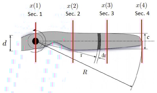
Figure 1.
Design variables for a candidate solution where d is and R is . are related to the airfoil sections [30,31].
The constraint-handling technique used either the constraint-based non-dominated sorting technique [56] or constraint dominance principles. Under these principles, the following points occur: (i) feasible solutions are prioritized over infeasible ones; (ii) among infeasible solutions, those with smaller constraint violations are ranked higher; and (iii) among feasible solutions, dominance determines the ranking. In the computational experiments conducted here, the algorithms were configured according to the parameters specified in their original references.
The power in Equation (1) is calculated using the BEM aerodynamic model. This model combines two principles: the momentum theory, from the actuator disk theory, which analyzes the change in airflow momentum through the rotor to estimate the thrust and power, and the blade element theory, which divides the blade into small sections (elements) along the radius and calculates the aerodynamic forces (lift and drag) on each section based on local flow conditions. BEM balances the forces from momentum conservation with the forces from blade aerodynamics to compute key quantities like thrust, torque, and power.
The relative velocity at a blade element is the magnitude of the vector sum of the axial wind velocity component and the tangential velocity due to rotor rotation. It is given by Equation (14), where is the free-stream wind speed, a is the axial induction factor, is the tangential induction factor, and is the rotor angular velocity (rad/s) (related to design variable, expressed in rpm). The power is expressed by the non-dimensional power coefficient of Equation (15), where P is the power extracted by the rotor, which has to be minimized for the flight conditions specified in Equation (1), is the air density, n is the rotational speed in revolutions per second (related to design variable, expressed in rpm), and D is the propeller diameter (design variable ).
The power in Equation (1) is calculated in terms of blade element aerodynamic parameter which depends on the angle of attack () and blade airfoil design, by a numerical integration across the blade span using local aerodynamic data (lift and drag coefficients of each airfoil).
The takeoff rotational speed point is found using the designed propeller by changing the pitch angle and rotational speed, looking for the lowest possible power within the limits. The function has a value of 1 when the Mach number at the propeller tip assumes values equal to or greater than and a value of 0 for smaller values. Such a function is important to prevent noisy propellers due to the creation of shock waves. Excessively thin or thick profiles have been removed from the database.
The diameter was set within limits of 1200 mm and 2000 mm. The number of possible blades was set from 4 to 13, and the hub diameter and total diameter ratio were limited from to .
3. The Optimization Framework
The optimization framework, called OptProp, starts by generating the initial population, which PlatEMO [53] carries out according to the corresponding evolutionary algorithm. Then, through the analyzed airfoils database, the objective function is evaluated for each initial population, and according to the specificity of the algorithm used, the next population is generated. This process is repeated until the stop criterion is reached. PlatEMO generates the Pareto fronts from the non-dominated propeller solutions when this iterative process is finished.
The main developments of this methodology comprise the creation and refinement of an extensive database of aerodynamic airfoils, the propeller analysis, and the development of a unifying algorithm for propeller analysis and optimization. The flowchart of the OptProp methodology is depicted in Figure 2, and detailed information can be found in Oliveira [30,31].
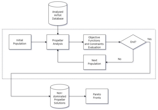
Figure 2.
Flowchart of the OptProp methodology [30,31].
3.1. Airfoil Database and Profiles Refinement
The initial phase of the proposed methodology involves establishing an extensive airfoil database, refining it, and conducting subsequent aerodynamic analysis. This was accomplished by compiling airfoil coordinates from the University of Illinois Urbana-Champaign (UIUC) [57]. The database comprises approximately 1600 airfoils, spanning various well-established families in the aeronautical field and literature, such as NACA, EPPLER, SELIG, Drela, Gottingen, and Wortmann. However, some thin, geometrically unfeasible, and poorly performing airfoils were excluded from the analysis, resulting in 4993 combinations of airfoils and Reynolds numbers.
The airfoils obtained from the UIUC database exhibit variations in the number of coordinate points. Airfoil aerodynamic analyses were conducted using XFOIL 6.94 [45], interactive software designed to analyze and design isolated airfoils. During aerodynamic analysis, airfoils with an insufficient number of points face challenges in convergence, leading to a decrease in result reliability. Given the absence of strict standardization in the data presentation, it becomes imperative to undertake data standardization processes and refine these airfoils by addressing the number of points in Cartesian coordinates.
An average of 200 points was designated for the refined airfoils to address this issue. Typically, XFOIL achieves satisfactory convergence with 100 to 150 points, as highlighted by Deperrois [58]. To generate the new interpolated points, a formulation based on ordinary differential equations describing the curve’s path was employed [59]. The points were strategically distributed to focus on the initial 15% of the airfoil chord in the upper and lower curves, constituting approximately 70% of the points. This approach was chosen due to the increased curvature near the leading edge, necessitating more points for smoother representation. Figure 3 visually depicts the refinement process.
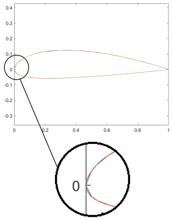
Figure 3.
Visualization of the refinement algorithm results on an airfoil, where the orange line represents the refinement geometry [30,31].
Following the enhancement of this dataset, aerodynamic analyses of the refined airfoils were conducted. For each initial airfoil derived from the UIUC Airfoil Coordinates Database, the analysis encompassed the following criteria: an angle of attack ranging from to with a 0. increment; Reynolds numbers at , , , and ; and forced transitions at both top and bottom boundary layers positioned at relative section positions per chord () equal to 1.00. The log of the amplification factor (NCrit) triggering transition for the panel method simulations was set to 9, the Mach number was 0, and the maximum number of iterations was set equal to 100.
3.2. Propeller Analysis
Four segments of the airfoil profile were chosen from the airfoil database for subsequent BEM analyses. The JavaProp model was chosen as the propeller aerodynamic tool [60,61,62,63]. It uses the tip loss factor derived from Prandtl’s theory to account for the effects of the free blade tip and the finite number of blades. Additionally, it incorporates momentum theory to correct for the induced velocity effects. The dimensionless positions of these sections and the airfoil sections’ specifications are detailed in Section 2 and visualized in Figure 1. Additionally, 9 profiles were interpolated between each pair of selected section profiles, resulting in 31 blade sections.
Out of the approximately 1600 profiles initially analyzed, 4993 polar files were generated. This increased number is due to certain combinations of airfoils and Reynolds numbers that could not produce results through the panel method analysis. Despite conducting analyses within the to angle of attack range, many profiles did not yield results across the entire analysis span. To address this, specific angle ranges were defined for the selected sections.
A comparable analysis is conducted based on the Reynolds number. Following the calculation of the Reynolds number for one of the four sections, the algorithm seeks the base Reynolds number (, , , or ) that is geometrically closest to the calculated Reynolds number for the section. Similar to the angle of attack range, the Reynolds number for each section is employed as a constraint.
It is essential to highlight that the BEM aerodynamic model implemented in the JavaProp platform [60] is a low-fidelity model that assumes steady flow around the propeller blades. Additionally, some airfoil curves generated with XFOIL fail to converge at extreme angles of attack, rendering them invalid. Despite these limitations, the model is well-established in the literature [61,62,63] and offers a balance between computational efficiency and analysis detail, making it suitable for preliminary design and optimization without requiring extensive computational resources. Furthermore, the aerodynamic contributions of the aircraft components are not included in the analysis.
3.3. Coupling the Propeller Aerodynamic Analysis and the Optimization Process
The third phase involves the integration of the optimization algorithms with the propeller solver, as depicted in Figure 2. Using a set of predefined design variables, multiple propellers are generated (initial population), analyzed (propeller analysis), and assessed based on the defined objectives (objective functions evaluation). This iterative process continues until convergence is reached, resulting in a set of non-dominated propeller solutions and corresponding Pareto fronts.
The propeller analysis phase assesses the objective functions, taking into account the propeller’s aerodynamic and geometric characteristics. Equation (1) determines the combination of objective functions.
The design variables correspond to the definitions specified in the formulations of the MOOPs, as expressed in Equations (9)–(13), and illustrated in Figure 1. These design variables encapsulate the aerodynamic details of the given airfoil, including the polar file configuration, angle of attack range definition, Reynolds number specification, and identification of the angle with the maximum lift-to-drag ratio.
A candidate solution within the optimization process, representing a complete propeller definition, is determined through the following steps: (i) selection of four sections from the airfoil database as design variables; (ii) interpolation between consecutive sections, resulting in the airfoil being an interpolated shape between the two closest section airfoils; and (iii) complete propeller definition using the last four design variables: propeller diameter, number of blades, hub diameter per propeller diameter, and rotational speed.
4. Structural Model for a Rotating Beam
This section describes the rotating beam model to perform the modal analysis of the propeller blades. As tapered rotating cantilever beams, propeller blades experience changes in their natural frequencies of vibration due to the rotor rotation. Assessing how this frequency interacts with engine rotation can predict the no-go zones. The no-go zones, in the context of the Campbell diagram, are areas where the excitation frequencies of the rotating system intersect with the natural frequencies of vibration of the system. Accessing and avoiding the regions where resonance occurs is critical for ensuring operational stability.
The method employed builds on the approach introduced by Rao and Gupta [13]. Their model computes stiffness and mass matrices for a rotating, warped, and tapered beam element with rectangular cross-sections, incorporating shear effects. However, this work excludes shear effects, as they are considered negligible for the analysis, and extends the model to accommodate non-rectangular cross-sections, such as those found in propeller blades.
Key features of the model include bending degrees of freedom in both the yz and xz planes, interpolated using Hermite polynomials, as illustrated in Figure 4. The total beam strain energy is minimized based on the finite element framework provided by Rao and Gupta [13]. The model also integrates cross-sectional variations, where area and moment of inertia functions are expressed as linear relationships concerning the beam length (z).
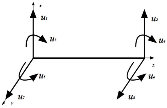
Figure 4.
Bending degrees of freedom.
By considering the geometry and warp angle of the structure, the stiffness and mass matrices are formulated. The airfoil sections are assumed to be solid. The cross-section area of an element changes with z and is given by Equations (16) and (17).
where and are the areas of the element’s left and right cross-sections, and l is the element length.
The moment of inertia functions after applying the warp angle can be written through angular transformations of the moment of inertia values given in the main axes of inertia. In this way, the values between the elements can be obtained using Equations (18)–(20).
where xx and yy refer to the main axes of inertia, and x’x’ and y’y’ are axes inclined by the warp angle .
The use of a rotating beam model in this study enables the modal analysis of the blade structure, which is considered as a rotating cantilever. This model was developed to extract the modal characteristics of the structure, with a primary focus on its natural frequencies in the bending modes. Since this is a modal analysis, the structural model does not require information about aerodynamic loads, nor does it assess the stresses and deformations they induce.
Boundary conditions specific to a cantilever beam are then applied to derive the global matrices. An eigenvalue and eigenvector problem arises with the stiffness, mass matrices, and boundary conditions. The eigenvalues represent the natural frequencies, which, when combined with the Campbell diagram, identify the no-go zones regions that should be avoided during the operational analysis of the propeller to prevent structural instabilities.
5. Optimum Design of the Propellers
Mission data from a turboprop aircraft with two engines were used for the optimization. The chosen optimization points of takeoff and top-of-climb are presented in Table 2. Thrust, speed, and altitude were adapted from Bermperis et al. [54].
Table 2.
The chosen optimization points of takeoff and top-of-climb.
5.1. Design Space Exploration
The formulation of the multi-objective optimization problem was defined in Section 2 with two different conflicting objective functions, which are to minimize the power at the takeoff point (PowerToff) and the top-of-climb point (PowerTOC).
In this section, we seek to understand how such objectives will behave with the variation of design variables through design space exploration. The first four design variables adopted are related to the airfoils used in four different propeller stations. As two airfoils of neighboring indexes can have completely different characteristics, exploring these first four design variables is not feasible. Therefore, the variables of propeller diameter, number of blades, and the ratio between the hub diameter and the propeller diameter will be adopted for design space exploration. The data presented in this section through the figures were obtained via numerical simulation.
The first two design exploration charts are depicted in Figure 5 and Figure 6. In these cases, the influences of the number of blades and diameter on the takeoff and top-of-climb powers were observed. Figure 5 shows that the diameter greatly influences the value of the top-of-climb power, and the greater the value, the smaller the objective in question. The increase in the number of blades also causes a drop in the objective value, but in a more subtle way.
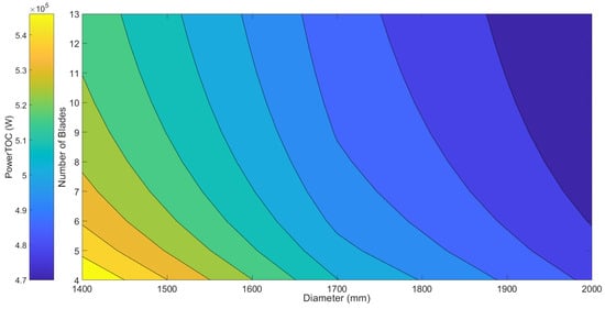
Figure 5.
Design exploration—number of blades × diameter: PowerTOC.
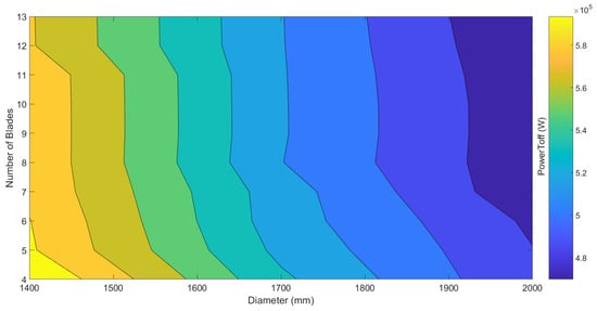
Figure 6.
Design exploration—number of blades × diameter: PowerToff.
Observing Figure 6, it can be seen that here, too, the increase in diameter leads to a significant drop in the value of takeoff power. The increase in the number of blades also causes a drop in the value of the objective, but even more modestly than in the power at the top-of-climb.
Figure 7 and Figure 8 place the hub/diameter ratio and diameter variables in design exploration for the two objective powers. In Figure 7, it can be seen that, again, the diameter has a great influence on the top-of-climb power. Within the analysed range, increasing the hub/diameter ratio causes a small increase in the objective. Figure 8 shows similar results for the PowerToff.
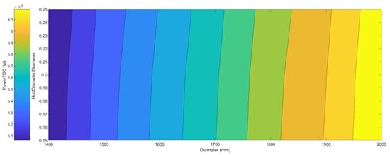
Figure 7.
Design exploration—hub/diameter ratio: PowerTOC.
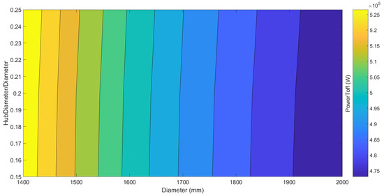
Figure 8.
Design exploration—hub/diameter ratio: PowerToff.
Through the design exploration, it is understood that increasing the diameter and number of blades and decreasing the hub/diameter ratio will minimize both objectives. The main variable of influence found was the diameter, so the larger this variable is, the smaller the minimized objectives. In the first instance, one might think that propellers with a diameter at the upper limit will be selected, but some constraints, such as the Mach number at the propeller’s tip, will limit this variable.
5.2. Solutions Obtained from the Optimization Problem
Thrust, Mach number, and altitude for the design points are set on the objective function. The properties related to the change in altitude, such as air density, kinematic viscosity, and the speed of sound, were also considered. Due to the good results demonstrated by Oliveira et al. [30], the NSGAII, AGEMOEA, and ARMOEA algorithms were adopted. For each run, 10,000 solutions were evaluated across 100 generations and a population with 100 individuals. Five independent runs were performed for each of the three algorithms, thus totaling 150,000 solutions. These runs took approximately 125 h and were performed on two computers, with Intel Core i7-11800H and Intel Core i7-7700HQ processors. The Pareto front for propeller optimization: PowerTOC × PowerToff is provided in Figure 9.
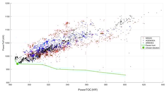
Figure 9.
Final population for the propeller optimization: PowerTOC × PowerToff, and extracted solution.
From Figure 9, one can observe that there is a tendency for the best solutions to be as good for PowerTOC as for PowerToff. The final population of the evolutionary computation demonstrates a vast volume of possible designs that synergetically minimize power at takeoff and top-of-climb conditions, whilst a small set of points illustrates a weak tradeoff in the form of a sparsely populated Pareto front. This results from the multi-objective process, addressing potential tradeoffs between these two critical design conditions. Still, the improvement in takeoff power is marginal along the sparse Pareto. Consequently, the design chosen in this study belongs to the interface between the strong synergetic cloud of solutions and the weak Pareto. In this case, a robust design is employed for the subsequent sections of this study. Even so, the multi-objective analysis would still be interesting, so it would not be necessary to carry out multiple single-objective optimizations.
It is also possible to see from Figure 9 that ARMOEA performed well in creating a large density of points to the left of the graph, providing solutions with lower powers at the top-of-climb, while NSGAII and AGEMOEA were able to find some points further down the graph, therefore providing solutions with lower takeoff powers. The propeller was selected by inspection and is indicated in the green circle in Figure 9, as it exhibited low values at the two objectives studied.
The selected propeller has the following characteristics, related to the design variables of Figure 1:
- Airfoil profile in Sec. 1 (design variable x(1)): FX 74-CL6-140, a high lift, low drag, and smooth stall behavior airfoil [64].
- Airfoil profile in Sec. 2 (design variable x(2)): NPL ARC CP 1372, a low drag, gradual stall, and with good lift-to-drag ratio airfoil [65].
- Airfoil profile in Sec. 3 (design variable x(3)): NACA 65(3)-218, a high lift, higher drag at high speeds, and steep stall airfoil [66].
- Airfoil profile in Sec. 4 (design variable x(4)): NACA M5, a low drag, good lift-to-drag, and mild stall behavior airfoil.
- propeller diameter (design variable x(5)): 1879 mm.
- number of blades (design variable x(6)): 8.
- hub diameter to propeller diameter ratio (design variable x(7)): .
- rotational speed (design variable x(7)): 1337.
An important point to highlight is that, within the OptProp framework, a database containing the polarities of various airfoils designed for different aerodynamic applications was provided at the beginning of the optimization process. Additionally, the definition of upper and lower limits for the design variables was intended to promote a diverse set of non-dominated solutions. This approach effectively expanded the range of options available to optimization algorithms. As a result, the solution derived from the optimization process selected design choices that, in conventional practices, would not typically be considered. It should be emphasized that the OptProp multi-objective methodology was consistent in providing simultaneously optimized solutions for two critical points of the flight, takeoff and top-of-climb. Moreover, the variety of solutions generated through this multi-objective optimization makes direct comparisons with existing solutions challenging due to variations in the underlying scenarios [52].
The angle distribution, the chord distribution, and a three-dimensional drawing of the selected propeller can be seen in Figure 10, Figure 11 and Figure 12.
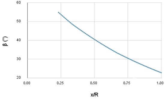
Figure 10.
Twist angle of the selected propeller along the chord–radius ratio.
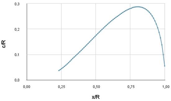
Figure 11.
Chord along the radius of the selected propeller along the chord–radius ratio.
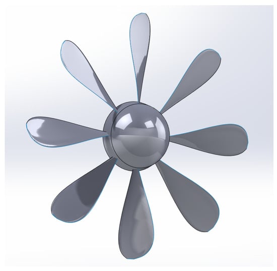
Figure 12.
Tridimensional geometry of the selected propeller.
6. Optimal Operational Procedures of the Optimized Propeller for a Given Flight Mission and with Structural Constraints
6.1. Operational Evaluation
This section proposes a comparative study of two different procedures in mission. In both cases, data related to the same standard mission of a turboprop aircraft divided into 103 different steps are considered. In Figure 13, it is possible to see how the altitude varies during the mission. Mission data was based on a turboprop aircraft and adapted from Bermperis et al. [54].
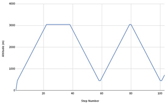
Figure 13.
Altitude versus flight mission step.
The mission can be divided into the following phases: (1) Takeoff: Step 1; (2) Climb: Steps 2–22; (3) Cruise: Steps 23–37; (4) Descent: Steps 38–58; (5) Second Climb: Steps 59–79; (6) Second Descent: Steps 80–100; and (7) Hold: Steps 101–103.
The first four phases can be considered a typical mission for a turboprop aircraft. Phases 5–7 refer to a situation where, for whatever reason, the aircraft cannot land and needs to regain its altitude to maneuver for the next landing. To carry out such a mission, the required values of aircraft velocity and thrust shown in Figure 14 and Figure 15 must be achieved in each of the steps of the mission. The values shown for thrust are relative to each of the two engines, so the total aircraft thrust value is double that shown below.
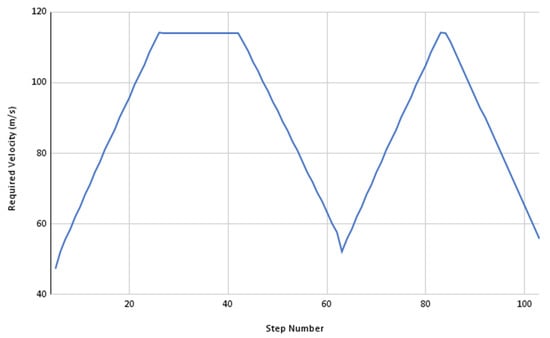
Figure 14.
Velocity versus flight mission step.
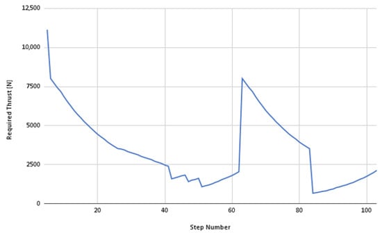
Figure 15.
Thrust versus flight mission step.
The propeller optimized in Section 6 was considered to carry out these missions. The first mission philosophy, which is going to be called 3-rotational-speed flight, considers something that is already quite conventional in the current aeronautical industry, which is the use of three different points for the engines’ rotational speed. The second mission philosophy, called multi-rotational-speed flight, aims to use different values of rotational speed to minimize the power in each of the mission steps. Such a philosophy is not conventional in the aeronautical industry; however, it generates power savings and, therefore, fuel savings. This section aims to demonstrate and measure this economy using different propeller rotational speeds throughout the flight mission. For this, in addition to the rotational speed changing at every step of the flight, it is also necessary to change the pitch angle of the propeller blades.
In this way, both mission philosophies were executed, and the results for propeller rotational speeds are shown in Figure 16. In the case of 3-rotational-speed flight, the rotational speed levels and the pitch angles were found, which minimize the power for each step. The same was done for the multi-rotational-speed flight case. It can be seen when comparing Figure 15 and Figure 16 that there is a shape correlation between the required thrust and rotational speed for the multi-rotational-speed flight case.
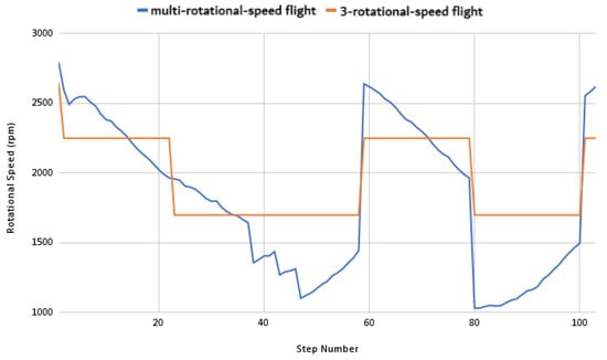
Figure 16.
Propeller rotational speeds (rpm) for both philosophies.
Figure 17 shows the power percentage difference between the multi-rotational-speed approach and the 3-rotational-speed approach, normalized by the 3-rotational-speed power. There is no difference at some points, but at others, it can reach almost . These results represent the power savings when the multi-rotational-speed approach is used. One can observe that continuously varying the propeller’s rotational speed can result in immediate power savings of up to 10 while maintaining overall energy demands. This is an important achievement, since, especially in electrified propulsion systems, the peak power determines the size of electrical and thermal components.
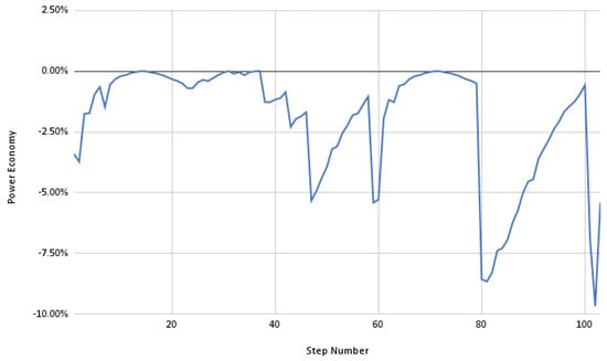
Figure 17.
Power economy comparing multi-rotational-speed flight and 3-rotational-speed flight.
Propeller efficiency () for both cases is shown in Figure 18. It is observed that these values are very close for both cases, with the multi-rotational-speed flight propeller efficiency showing a slightly higher efficiency in some regions. It is also possible to notice that the propeller efficiency is lower at points with high power requirements, such as takeoff and climb, and greater at points where the power requirement is lower, such as cruise and descent.
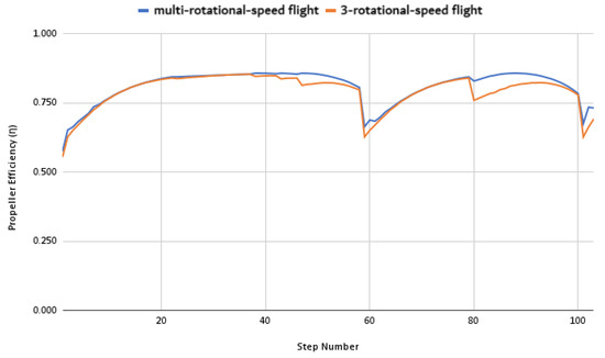
Figure 18.
Propeller efficiency () for multi-rotational-speed flight and 3-rotational-speed flight.
Figure 19 shows the variation of the coefficients of thrust () and power () along the flight for both cases. The values of the coefficients vary within the same range; however, the coefficient values for the multi-rotational-speed flight vary more smoothly than in the 3-rotational-speed flight case. Such behavior can be attributed to the condition that the propeller’s rotational speed can assume any value.
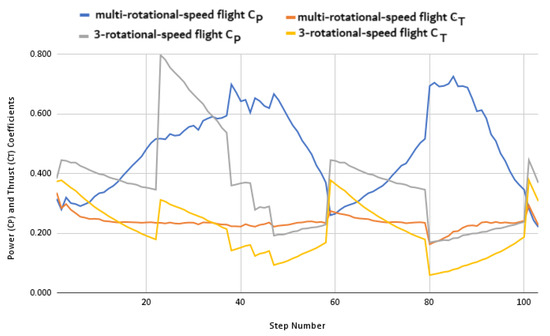
Figure 19.
Thrust () and power () coefficients for multi-rotational-speed flight and 3-rotational-speed flight.
Figure 20 shows how the twist angle at the of the blade span varies along the missions, for multi-rotational-speed flight and 3-rotational-speed flight. As expected, where the rotational speed values are the same for both cases (Steps 14–15, 22–23, 34–35, 58–59, 71–72, and 101–102) in Figure 16, the angle values are also the same in Figure 20.
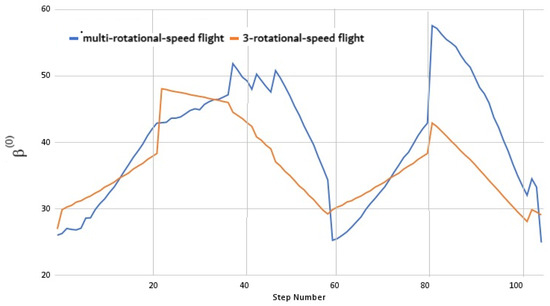
Figure 20.
Twist angle variation at 75% chord–radius ratio for multi-rotational-speed flight and 3-rotational-speed flight.
The total energy used in a flight mission can be evaluated using Equation (21).
where is the total energy for a mission, is the power, and is the time for each of the steps i. Therefore, the percentage energy savings can be written according to Equation (22).
where and are the total energies for the multi-rotational-speed flight and 3-rotational-speed flight procedures, respectively. Developing Equations (21) and (22):
where is the power at step i for the multi-rotational-speed approach and is the power at step i for the 3-rotational-speed approach.
Assuming that all time step values are equal, Equation (23) can be reduced to:
Applying the power values to Equation (24) saves of the proposed mission’s total energy, proving that the continuously multi-rotational-flight philosophy can generate economic gains. Depending on the type of mission, these power-saving values can be even greater, since the more erratic a flight is, the less suitable the fixed rotational speed bands will be. Therefore, multi-rotational-speed flight can mean even lower flight energies and therefore lower fuel consumption for more complex missions.
6.2. Operational Analysis Under Structural Constraints
This subsection presents the modal analysis of the optimized propeller obtained in Section 5 under structural frequency constraints. This constraint is essential to prevent resonance between the blade vibration modes and the rotor’s rotational motion and could prevent structural instability during the flight. The structural dynamic model to obtain its natural frequency of vibration is briefly explained in Section 4. The material was structural steel with Young modulus GPa and specific mass . Each blade was discretized using 25 beam elements.
The complete set of the natural numbers can be found in Table 3. The first column of Table 3 refers to the rotational speed of the propeller, and the flapwise and edgewise modes refer to the two main flexural modes of vibration. The analysis of the results indicates a significant impact of the propeller’s rotation on the natural frequencies of the blades. The increase in blade natural frequencies is attributed to the enhanced stiffness resulting from the centrifugal forces generated by the propeller’s rotation, justifying the structural model for a rotating beam employed in the research.
Table 3.
Natural frequencies of the blades.
The Campbell diagram, a graphical representation used in turbomachinery to illustrate the relationship between the natural frequencies of a rotating system and its rotational speed, is used to identify critical rotational speeds where resonance might occur. Figure 21 presents the Campbell diagram for the propeller, where the first four-engine orders were considered, with the engine order () equivalent to the number of blades, and twice the number of blades, that is, .
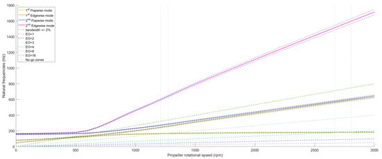
Figure 21.
Campbell diagram.
Figure 21 shows areas where the natural frequency curves intersect with the straight lines representing the engine order. These regions are called no-go zones since they are rotation regions in which the engines must not operate. Figure 22 evidences the region between 350 and 750 rpm. It is possible to notice in Figure 22 that in the region between 350 rpm and 750 rpm, there are some intersections between natural frequencies and = 16. However, as the engine only passes through these frequencies and does not operate in them continually in any part of the flight, for clarity on the chart, it was not marked as a no-go zone. At 1244 rpm, the first vibration frequency coincides with , and at 2736 rpm, the intersection between the first frequency and occurs. As these are rotation frequencies in the aircraft operating range, two no-go zones are generated considering a bandwidth of around the natural frequencies, resulting in the ranges of 1213 to 1275 rpm and 2668 to 2804 rpm, respectively.
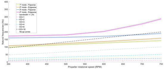
Figure 22.
Campbell diagram: 350–750 rpm range.
Therefore, two distinct prohibited zones are established in the Campbell diagram, which represent the regions where the propeller cannot operate: the ranges from 1213 to 1275 rpm and from 2668 to 2804 rpm. The superposition of this information on the multi-rotational-speed flight approach graph in Figure 16 reveals that the rotational speeds used in some segments fall within the prohibited zones. Specifically, these include Step 1 (takeoff), Steps 42, 52, and 53 (descent), and Steps 93 and 94 (second descent). This subsection analyzes the same propeller with the no-go zones operating restriction. To accomplish this, the rotations of the segments Step 1 (takeoff), Steps 42, 52, and 53 (descent), and Steps 93 and 94 (second descent) are swapped with the closest allowed rotation, and the aerodynamics data are recalculated. Table 4 presents the recalculated aerodynamic parameters along the mission when the structural constraint is considered. Figure 23 plots the new rotational speed profile for frequency-constrained multi-rotational speed flight missions, referred to as multi-rotational-speed-constrained. In this figure, the no-go zones between 1213 and 1275 rpm and between 2668 and 2804 rpm are labeled as No-Go Zone 1 and No-Go Zone 2, respectively. The 3-rotational-speed flight approach is also shown. During the new flight mission, the region corresponding to Prohibited Zone 2 is not reached at any point. Although there are two moments when the flight mission intersects prohibited zone 1, the propeller speed is promptly adjusted to the outer limits of this range to prevent resonance between its natural frequencies and the operating speeds.
Table 4.
New flight mission points considering structural constraints.
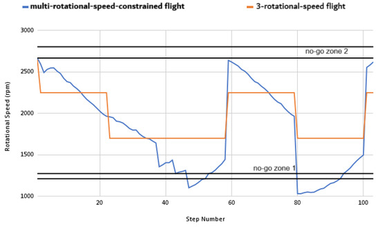
Figure 23.
Propeller rotational speeds (rpm) for no-go zones.
Figure 24 shows the power percentage difference between the multi-rotational-speed-constrained and 3-rotational-speed approaches, normalized by the 3-rotational-speed power, and using structural constraints. Due to the structural constraint applied and some segments no longer being in minimum power rotation, the energy saving obtained here is , slightly smaller than that obtained in Section 6.1 (), where there are no structural constraints. However, because few segments were affected by the constraint, there was no major change in energy savings. It is also possible to see from Figure 24 that in-flight stages with takeoff, climb, and descent, power savings vary between 3% and 10%.

Figure 24.
Power economy comparing multi-rotational-speed-constrained flight (with structural constraints) and 3-rotational-speed flight.
7. Final Considerations
This study introduced a multi-objective optimal design for aeronautical propellers, utilizing BEM theory and evolutionary algorithms. The OptProp framework facilitated the optimization of propeller design by focusing on minimizing power consumption during takeoff and at the top-of-climb. Also, an evaluation of variable rotational speed flight under structural constraints was presented. The main purpose of these developments is to reduce power consumption while maintaining performance and structural integrity.
Subsequently, the chosen propeller design was evaluated under optimal operational conditions for a specific mission. The process consisted of searching for the minimum power required for each mission point by varying the values of rotational speed and pitch angle. This process was performed with and without dynamic constraints, obtaining the general flight energy reduction values of and , respectively. This is a significant achievement, as continuous variation in propeller rotational speed can yield instantaneous power savings of up to 10%. Even at peak power conditions, substantial savings are found, particularly in electrified propulsion, where peak power dictates the sizing of electrical and thermal components. These approaches achieve power savings during critical flight stages without compromising overall energy requirements.
This is a novel proposal not found in existing references on the subject. Particularly, it is suited for application in conceptual propeller early-stage design. This suitability is supported by low-fidelity models, which prioritize practical and efficient analyses. The findings presented in this study validate these expectations, demonstrating a significant improvement in the propeller’s performance.
The main strengths of the proposed research can be highlighted as follows:
- The OptProp coupled methodology for propeller optimization, which allows the consideration of different propeller geometries, such as chord distribution and twist, in addition to the airfoil section.
- The proposed MOOP delivered an optimized propeller considering minimum energy consumption at two points of interest in the flight envelope, thus enabling the design of efficient propellers systematically and pragmatically. The results obtained demonstrate its potential, providing feasible non-dominated solutions and significantly reducing computational costs using the BEM theory.
- The application of the optimized propeller in a mission, evaluating the multi-rotational-speed flight procedure to mitigate the power consumption. Also, using the Campbell diagram to predict no-go zones could prevent structural instability during the flight.
- It corroborates the various studies in the area that aim to improve aeronautical systems’ efficiencies while trying to mitigate environmental and economic impacts.
This paper does not address practical considerations related to the manufacturing and implementation of the proposed propeller design. These aspects represent a natural direction for future work, which could benefit from advancements in propeller manufacturing technologies. Additionally, the aerodynamic model does not account for engine performance when reducing its rotation in the multi-speed flight approach. However, modern engines and powertrains, particularly those with variable-pitch propellers or hybrid systems, are being developed to maintain efficiency over a broader rotational range, mitigating these effects.
For future work, applying high-fidelity methods to the obtained propeller with multi-criteria decision-making is of great interest, especially when combined with surrogate-assisted (SA) models to reduce computational costs. Other improvement points include the the combination of BEM with SA models, the use of post-stall extrapolation methods for airfoil analysis, and the coupling of structural and aerodynamic models in the optimization process. This would enable the incorporation of not only natural frequencies but also stress and deformation analyses resulting from aerodynamic loading.
Author Contributions
Conceptualization: N.L.O., A.C.d.C.L., P.H.H., K.K., S.V. and M.A.R.; methodology: N.L.O., A.C.d.C.L., P.H.H. and S.V.; software: N.L.O. and S.V.; validation, N.L.O.; formal analysis: N.L.O., A.C.d.C.L., P.H.H., K.K., S.V. and M.A.R.; investigation: N.L.O.; resources: A.C.d.C.L., P.H.H. and K.K.; data curation: N.L.O.; writing—original draft preparation: N.L.O., A.C.d.C.L., P.H.H., K.K., S.V. and M.A.R.; visualization: N.L.O.; supervision: A.C.d.C.L., P.H.H., K.K. and S.V.; project administration: P.H.H. and K.K.; funding acquisition: P.H.H. and K.K. All authors have read and agreed to the published version of the manuscript.
Funding
This research was funded by Coordenação de Aperfeiçoamento de Pessoal de Nível Superior (Capes)—Finance Code 001; Fundação de Amparo à Pesquisa do Estado de Minas Gerais (Fapemig)—Grants TEC PPM-00174-18 and APQ-00869-22, and Conselho Nacional de Desenvolvimento Científico e Tecnológico (CNPq)—Grants 308105/2021-4 and 303221/2022-4.
Data Availability Statement
The data will be made available under request.
Acknowledgments
For academic development and guidance, the authors thank the Graduate Program in Computational Modeling (PGMC) at the Federal University of Juiz de Fora (UFJF), and the Future Energy Center (FEC) at Mälardalen University (MDU).
Conflicts of Interest
The authors declare no conflicts of interest. The funders had no role in the design of the study; in the collection, analyses, or interpretation of data; in the writing of the manuscript; or in the decision to publish the results.
References
- Misté, G.A.; Benini, E. Performance of a turboshaft engine for helicopter applications operating at variable shaft speed. In Gas Turbine India Conference; American Society of Mechanical Engineers: New York, NY, USA, 2012; Volume 45165, pp. 701–715. [Google Scholar]
- Garavello, A.; Benini, E. Preliminary study on a wide-speed-range helicopter rotor/turboshaft system. J. Aircr. 2012, 49, 1032–1038. [Google Scholar] [CrossRef]
- Vouros, S. Aeroacoustic Simulation of Rotorcraft Propulsion Systems. Ph.D. Thesis, Cranfield University, College Rd, Wharley End, Bedford, UK, 2024. Available online: https://dspace.lib.cranfield.ac.uk/handle/1826/20073 (accessed on 2 June 2025).
- Vouros, S.; Goulos, I.; Pachidis, V. Integrated methodology for the prediction of helicopter rotor noise at mission level. Aerosp. Sci. Technol. 2019, 89, 136–149. [Google Scholar] [CrossRef]
- Polyzos, N.D.; Vouros, S.; Goulos, I.; Pachidis, V. Multi-disciplinary optimization of variable rotor speed and active blade twist rotorcraft: Trade-off between noise and emissions. Aerosp. Sci. Technol. 2020, 107, 106356. [Google Scholar] [CrossRef]
- Scullion, C.; Vouros, S.; Goulos, I.; Nalianda, D.; Pachidis, V. Optimal control of a compound rotorcraft for engine performance enhancement. J. Eng. Gas Turbines Power 2021, 143, 021005-1. [Google Scholar] [CrossRef]
- Wald, Q. The aerodynamics of propellers. Prog. Aerosp. Sci. 2006, 42, 85–128. [Google Scholar] [CrossRef]
- Sodja, J.; Stadler, D.; Kosel, T. Computational fluid dynamics analysis of an optimized load-distribution propeller. J. Aircr. 2012, 49, 955–961. [Google Scholar] [CrossRef]
- Loureiro, E.V.; Oliveira, N.L.; Hallak, P.H.; de Souza Bastos, F.; Rocha, L.M.; Delmonte, R.G.P.; de Castro Lemonge, A.C. Evaluation of low fidelity and cfd methods for the aerodynamic performance of a small propeller. Aerosp. Sci. Technol. 2021, 108, 106402. [Google Scholar] [CrossRef]
- Gur, O.; Rosen, A. Optimization of propeller based propulsion system. J. Aircr. 2009, 46, 95–106. [Google Scholar] [CrossRef]
- Bergmann, O.; Möhren, F.; Braun, C.; Janser, F. Aerodynamic design of swept propeller with bemt. DLRK 2022, 1–7. [Google Scholar]
- Hoyos, J.D.; Jiménez, J.H.; Echavarría, C.; Alvarado, J.P.; Urrea, G. Aircraft propeller design through constrained aero-structural particle swarm optimization. Aerospace 2022, 9, 153. [Google Scholar] [CrossRef]
- Rao, S.; Gupta, R. Finite element vibration analysis of rotating Timoshenko beams. J. Sound Vib. 2001, 242, 103–124. [Google Scholar] [CrossRef]
- Bergmann, O.; Möhren, F.; Braun, C.; Janser, F. On the influence of elasticity on swept propeller noise. In Proceedings of the AIAA SCITECH 2023 Forum, National Harbor, MD, USA & Online, 23–27 January 2023; p. 0210. [Google Scholar]
- Zhang, Y.; Fu, Y.; Wang, P.; Chang, M. Aerodynamic configuration optimization of a propeller using Reynolds-averaged Navier–Stokes and adjoint method. Energies 2022, 15, 8588. [Google Scholar] [CrossRef]
- Ahmad, F.; Kumar, P.; Patil, P.P.; Kumar, V. Design and modal analysis of a quadcopter propeller through finite element analysis. Mater. Today Proc. 2021, 46, 10322–10328. [Google Scholar] [CrossRef]
- Praveen, L.; Anoop, M.S. Modeling and finite element analysis of composite propeller blade for aircraft. AIP Conf. Proc. 2021, 2317, 020027. [Google Scholar]
- Al-Haddad, L.A.; Jaber, A.A. Influence of operationally consumed propellers on multirotor uavs airworthiness: Finite element and experimental approach. IEEE Sens. J. 2023, 23, 11738–11745. [Google Scholar] [CrossRef]
- Guan, G.; Zhang, X.; Wang, P.; Yang, Q. Multi-objective optimization design method of marine propeller based on fluid-structure interaction. Ocean Eng. 2022, 252, 111222. [Google Scholar] [CrossRef]
- Hussain, M.; Abdel-Nasser, Y.; Banawan, A.; Ahmed, Y.M. Fsi-based structural optimization of thin bladed composite propellers. Alex. Eng. J. 2020, 59, 3755–3766. [Google Scholar] [CrossRef]
- Eberhart, R.; Kennedy, J. A new optimizer using particle swarm theory. In MHS’95, Proceedings of the Sixth International Symposium on Micro Machine and Human Science, Nagoya, Japan, 4–6 October 1995; IEEE: New York, NY, USA, 1995; pp. 39–43. [Google Scholar]
- Holland, J.H. Genetic algorithms. Sci. Am. 1992, 267, 66–73. [Google Scholar] [CrossRef]
- Deb, K.; Agrawal, S.; Pratap, A.; Meyarivan, T. A fast elitist non-dominated sorting genetic algorithm for multi-objective optimization: Nsga-ii. In International Conference on Parallel Problem Solving From Nature; Springer: Berlin/Heidelberg, Germany, 2000; pp. 849–858. [Google Scholar]
- Panichella, A. An adaptive evolutionary algorithm based on non-euclidean geometry for many-objective optimization. In Proceedings of the Genetic and Evolutionary Computation Conference, Prague, Czech Republic, 13–17 July 2019; pp. 595–603. [Google Scholar]
- Tian, Y.; Cheng, R.; Zhang, X.; Cheng, F.; Jin, Y. An indicator-based multiobjective evolutionary algorithm with reference point adaptation for better versatility. IEEE Trans. Evol. Comput. 2017, 22, 609–622. [Google Scholar] [CrossRef]
- Hughes, E.J. MSOPS-II: A general-purpose many-objective optimiser. In Proceedings of the 2007 IEEE Congress on Evolutionary Computation, Singapore, 25–28 September 2007; pp. 3944–3951. [Google Scholar]
- Gur, O.; Rosen, A. Design of quiet propeller for an electric mini unmanned air vehicle. J. Propuls. Power 2009, 25, 717–728. [Google Scholar] [CrossRef]
- Ingraham, D.; Gray, J.S.; Lopes, L.V. Gradient-based propeller optimization with acoustic constraints. In Proceedings of the AIAA Scitech 2019 Forum, San Diego, CA, USA, 7–11 January 2019; p. 1219. [Google Scholar]
- Yu, P.; Peng, J.; Bai, J.; Han, X.; Song, X. Aeroacoustic and aerodynamic optimization of propeller blades. Chin. J. Aeronaut. 2020, 33, 826–839. [Google Scholar] [CrossRef]
- Oliveira, N.L.; Rendón, M.A.; de Castro Lemonge, A.C.; Hallak, P.H. Multi-objective optimum design of propellers using the blade element theory and evolutionary algorithms. Evol. Intell. 2023, 17, 1623–1653. [Google Scholar] [CrossRef]
- Oliveira, N.L. Optimizing Propeller Performance: A Comprehensive Constrained Multi-Objective Design Approach Using Blade Element Theory and Evolutionary Algorithms. Ph.D. Thesis, Federal University of Juiz de Fora, Juiz de Fora, Brazil, 2023. [Google Scholar]
- Yang, X.; Ma, D.; Zhang, L.; Yu, Y.; Yao, Y.; Yang, M. High-fidelity multi-level efficiency optimization of propeller for high altitude long endurance uav. Aerosp. Sci. Technol. 2023, 133, 108142. [Google Scholar] [CrossRef]
- Koyuncuoglu, H.; He, P. Cfd based multi-component aerodynamic optimization for wing propeller coupling. In Proceedings of the AIAA SCITECH 2023 Forum, National Harbor, MD, USA & Online, 23–27 January 2023; p. 1844. [Google Scholar]
- Geng, X.; Liu, P.; Hu, T.; Qu, Q.; Dai, J.; Lyu, C.; Ge, Y.; Akkermans, R.A. Multi-fidelity optimization of a quiet propeller based on deep deterministic policy gradient and transfer learning. Aerosp. Sci. Technol. 2023, 137, 108288. [Google Scholar] [CrossRef]
- Sedelnikov, A.; Kurkin, E.; Quijada-Pioquinto, J.G.; Lukyanov, O.; Nazarov, D.; Chertykovtseva, V.; Kurkina, E.; Hoang, V.H. Algorithm for propeller optimization based on differential evolution. Computation 2024, 12, 52. [Google Scholar] [CrossRef]
- Wu, X.; Zuo, Z.; Ma, L.; Zhang, W. Multi-fidelity neural network-based aerodynamic optimization framework for propeller design in electric aircraft. Aerosp. Sci. Technol. 2024, 146, 108963. [Google Scholar] [CrossRef]
- Weigang, A.; Tianyu, L.; Shigen, W. Optimal structural design for a certain near-space composite propeller of airship using adaptive region division blending model. Chin. J. Aeronaut. 2024, 37, 301–316. [Google Scholar]
- Glauert, H. The Elements of Aerofoil and Airscrew Theory, 2nd ed.; Cambridge University Press: Cambridge, UK, 1983. [Google Scholar]
- Theodorsen, T. Theory of Propellers, 1st ed.; McGraw-Hill: New York, NY, USA, 1948. [Google Scholar]
- Larrabee, E.E. Propellers of minimum induced loss, and water tunnel tests of such a propeller. In Proceedings of the NASA, Industry, University, General Aviation Drag Reduction Workshop, NASA Conference Publication, Lawrence, KS, USA, 1 January 1975; pp. 273–293. [Google Scholar]
- Larrabee, E.E.; French, S.E. Minimum induced loss windmills and propellers. J. Wind. Eng. Ind. Aerodyn. 1983, 15, 317–327. [Google Scholar] [CrossRef]
- Adkins, C.N.; Liebeck, R.H. Design of optimum propellers. In Proceedings of the AIAA 21st Aerospace Sciences Meeting, AIAA Aviation, Reno, NV, USA, 10 January 1983; p. 9. [Google Scholar]
- Drela, M. Qprop User Guide. 2007. Available online: http://web.mit.edu/drela/Public/web/qprop/qprop_doc.txt (accessed on 2 June 2025).
- Drela, M.; Giles, M.B. Viscous-inviscid analysis of transonic and low reynolds number airfoils. AIAA J. 1987, 25, 1347–1355. [Google Scholar] [CrossRef]
- Drela, M.; Youngren, H. Xfoil 6.94 User Guide. 2001. Available online: https://web.mit.edu/drela/Public/web/xfoil/xfoil_doc.txt (accessed on 2 June 2025).
- Malki, R.; Williams, A.; Croft, T.; Togneri, M.; Masters, I. A coupled blade element momentum–computational fluid dynamics model for evaluating tidal stream turbine performance. Appl. Math. Model. 2013, 37, 3006–3020. [Google Scholar] [CrossRef]
- Kovačević, A.; Svorcan, J.; Hasan, M.S.; Ivanov, T.; Jovanović, M. Optimal propeller blade design, computation, manufacturing and experimental testing. Aircr. Eng. Aerosp. Technol. 2021, 93, 1323–1332. [Google Scholar] [CrossRef]
- Toman, U.T.; Hassan, A.-K.S.; Owis, F.M.; Mohamed, A.S. Blade shape optimization of an aircraft propeller using space mapping surrogates. Adv. Mech. Eng. 2019, 11, 1687814019865071. [Google Scholar] [CrossRef]
- Alshahrani, A. Analysis and Initial Optimization of the Propeller Design for Small, Hybrid-electric Propeller Aircraft. Ph.D. Thesis, Aeronautical and Vehicle Engineering KTH Royal Institute of Technology, Stockholm, Sweden, 2020. [Google Scholar]
- Moreira, C.; Herzog, N.; Breitsamter, C. Wind tunnel investigation of transient propeller loads for non-axial inflow conditions. Aerospace 2024, 11, 274. [Google Scholar] [CrossRef]
- Denholm, T.J.; Sian, G.; Wisniewski, C. Geometric and material improvements to quiet propeller design. In Proceedings of the AIAA SCITECH 2024 Forum, Orlando, FL, USA, 8–12 January 2024; p. 0131. [Google Scholar]
- de Moura Ribeiro, A.; Hallak, P.H.; de Castro Lemonge, A.C.; dos Santos Loureiro, F. Automatic grouping of wind turbine types via multi-objective formulation for nonuniform wind farm layout optimization using an analytical wake model. Energy Convers. Manag. 2024, 315, 118759. [Google Scholar] [CrossRef]
- Tian, Y.; Cheng, R.; Zhang, X.; Jin, Y. Platemo: A Matlab platform for evolutionary multi-objective optimization [educational forum]. IEEE Comput. Intell. Mag. 2017, 12, 73–87. [Google Scholar] [CrossRef]
- Bermperis, D.; Ntouvelos, E.; Kavvalos, M.D.; Vouros, S.; Kyprianidis, K.G.; Kalfas, A.I. Synergies and trade-offs in hybrid propulsion systems through physics-based electrical component modeling. J. Eng. Gas Turbines Power 2024, 146, 011005. [Google Scholar] [CrossRef]
- Bermperis, D.; Kavvalos, M.D.; Vouros, S.; Kyprianidis, K.G. Advanced Power Management Strategies for Complex Hybrid-Electric Aircraft. In Turbo Expo: Power for Land, Sea, and Air; American Society of Mechanical Engineers: New York, NY, USA, 2024. [Google Scholar]
- Deb, K.; Pratap, A.; Agrawal, S.; Meyarivan, T. A fast and elitist multiobjective genetic algorithm: NSGA-II. IEEE Trans. Evol. Comput. 2002, 2, 182–197. [Google Scholar] [CrossRef]
- Selig, M. UIUC Airfoil Coordinates Database. 2020. Available online: https://m-selig.ae.illinois.edu/ads/coord_database.html (accessed on 12 September 2020).
- Deperrois, A. Xflr5 Analysis of Foils and Wings Operating at Low Reynolds Numbers, Guidelines for XFLR5 142; 2009. Available online: https://www.researchgate.net/profile/Mohamed-Mourad-Lafifi/post/Bravo_UAV_half_scale_trainer_analysis/attachment/5feb27c23b21a200016534c5/AS%3A974065238032385%401609246658631/download/XFLR5AnalysisoffoilsandwingsoperatingatlowReynoldsnumbers.pdf (accessed on 2 June 2025).
- D’Errico, J. Interparc Function, MATLAB Central File Exchange. 2012. Available online: https://www.mathworks.com/matlabcentral/fileexchange/34874-interparc (accessed on 2 June 2025).
- Hepperle, M. JavaProp Users Guide; Tech. Rep. 2010. Available online: https://www.mh-aerotools.de/airfoils/java/JavaProp%20Users%20Guide.pdf (accessed on 2 June 2025).
- Cornwell-Arquitt, L.A.; Curtis, C.G.; Albertani, R. Design, manufacturing, and testing of a propeller for solar-powered unmanned aerial vehicles. In Proceedings of the 2023 Regional Student Conferences, Multiple Locations, USA, 1 January 2023; p. 72204. [Google Scholar]
- Faraaz, M.; Faizan, A.; Badarinath, M.; Subramaniyan, K.V.; Harursampath, D.; Gupta, R.B. Baseline design of propeller for an evtol aircraft to achieve urban air mobility. In Proceedings of the 2023 IEEE Aerospace Conference, Big Sky, MT, USA, 4–11 March 2023; pp. 1–10. [Google Scholar]
- Crain, A.D.; Zdunich, P.; Canteenwalla, P.; MacRae, N. Hybrid electric aircraft testbed: Sizing and simulations of an electric propulsion system and energy storage system. AIAA Aviat. Forum Ascend 2024, 2024, 3703. [Google Scholar]
- McMasters, J.; Henderson, M. Low-speed single-element airfoil synthesis. Tech. Soar. 1980, 6, 1–21. [Google Scholar]
- Lovell, D.A. A Wind-Tunnel Investigation of the Effects of Flap Span and Deflection Angle, Wing Planform and a Body on the High-lift Performance of a 280 Swept Wing; Aeronautical Research Council: Cranfield, UK, 1977. [Google Scholar]
- Abbott, I.H.; Von Doenhoff, A.E.; Stivers, L., Jr. Summary of Airfoil Data; National Advisory Committee For Aeronautics: Washington, DC, USA, 1945. [Google Scholar]
Disclaimer/Publisher’s Note: The statements, opinions and data contained in all publications are solely those of the individual author(s) and contributor(s) and not of MDPI and/or the editor(s). MDPI and/or the editor(s) disclaim responsibility for any injury to people or property resulting from any ideas, methods, instructions or products referred to in the content. |
© 2025 by the authors. Licensee MDPI, Basel, Switzerland. This article is an open access article distributed under the terms and conditions of the Creative Commons Attribution (CC BY) license (https://creativecommons.org/licenses/by/4.0/).