A Dual-Level Intelligent Architecture-Based Method for Coupling Fault Diagnosis of Temperature Sensors in Traction Converters

Abstract

To address the coupled fault diagnosis challenge between temperature sensors and equipment in traction converter cooling systems, this paper proposes a dual-level intelligent diagnostic architecture. This method achieves online sensor fault isolation and early equipment anomaly warning by leveraging spatiotemporal correlation modeling of multimodal sensor data and ensemble learning-based prediction. At the first level, it integrates multi-source parameters such as outlet temperature and pressure to establish dynamic prediction models, which are combined with adaptive threshold mechanisms for detecting various sensor faults including offset, open-circuit, and noise interference. At the second level, it monitors the status of temperature sensors through time-series analysis of inlet temperature data. Verified on an edge computing platform, the proposed method effectively resolves the coupling misdiagnosis between sensor distortion and equipment faults while maintaining physical interpretability, thereby significantly enhancing diagnostic robustness under complex operating conditions.

1. Introduction

With the advancement of rail transit systems toward high-density and heavy-load operation, the reliability of traction converters has become a critical bottleneck affecting train operational safety and economic performance. As the core component for energy conversion, the power modules in converters generate thermal losses reaching megawatt levels under complex operating conditions [1]. The temperature monitoring network serves a dual role: acting as a real-time feedback channel for cooling system regulation and providing diagnostic features for equipment health assessment. However, the harsh operating conditions inherent to rail transit—such as high-frequency mechanical vibrations and strong electromagnetic interference—pose more severe reliability challenges for temperature sensors compared to industrial stationary scenarios. Sensor faults, such as drift or open-circuit faults, may cause the CCU (central control unit) to misinterpret the cooling system’s status, potentially leading to abnormal shutdowns due to redundant protection mechanisms or, worse, masking actual equipment failures and causing catastrophic accidents. Notably, substantive faults within converters, such as insulated gate bipolar transistor (IGBT) module breakdowns, also manifest as abnormal temperature parameters. This creates a dual diagnostic dilemma: determining whether anomalous signals stem from sensor failures or reflect genuine equipment faults.

In the field of converter ontology fault diagnosis, physical modeling methods based on voltage/current signal analysis [2,3,4] and data-driven approaches [5,6,7] have reached a relatively mature stage. However, both types of methods are premised on the ideal assumption that the sensor system is entirely reliable, which may lead to the risk of misdiagnosis when sensor faults co-occur with equipment failures. Specifically, existing methods generally overlook two critical scientific challenges: First, sensor faults and equipment faults are strongly coupled in the time-frequency domain, making single-dimensional diagnostic models prone to generating “false-positive” alarms; second, the nonlinear heat transfer characteristics of the cooling system during start–stop transients and overload conditions complicate efforts to accurately decouple the real temperature field from sensor aberration signals using traditional static models.

Sensors, as critical sensing units in industrial control systems, directly influence operational safety through their reliability. In recent years, sensor fault diagnosis technologies have rapidly advanced for various applications, including motor drives, power electronic converters, and traction systems.

(1)

Model-based methods

Model-based diagnostic methods achieve fault detection by constructing a dynamic system model and using an observer to generate residual signals [8]. These methods are widely applied in motor drives and power electronic systems. For instance, sliding mode observers [9,10,11] and Kalman filtering [12] enable current sensor fault detection by comparing the residuals of the feedback current with the reference value in matrix converter-permanent magnet synchronous motor (PMSM) drive systems. For induction motors and interior permanent magnet synchronous motors (IPMSMs), the strategy proposed by Dan et al. based on extended Kalman filtering (EKF) can simultaneously handle current and voltage sensor faults while reducing noise interference [13]. For the single-phase three-element current limiter (SPTL), Xu et al. designed a reduced-order observer [14], which resolves the coupling issue between sensor faults and IGBT open-circuit faults by reconstructing the system state and decoupling sensor faults from switching device faults via a state-space model. A mixed logic dynamic (MLD) model was established by Ge et al. to analyze the slope characteristics of residual change rates, combined with an adaptive threshold setting strategy, enabling the simultaneous differentiation of open-circuit faults in IGBTs and clamping diodes [15]. Additionally, a rapid sensor fault diagnosis method derived from parity space was proposed by Berriri et al., leveraging time-window redundancy and equivalent space analysis to ensure algorithm robustness against parameter variations while maintaining diagnostic effectiveness [16].

The model-driven approach offers advantages such as clear physical interpretability and suitability for systems requiring fast dynamic responses. However, its limitations include a reliance on precise mathematical models, sensitivity to parameter drift, and an accuracy that is heavily dependent on the precision of system models and parameter estimation.

(2)

Data-driven methods

Data-driven methods leverage extensive historical data to extract deep knowledge characterizing implicit relationships among system variables through statistical analysis or artificial intelligence techniques, thereby training diagnostic models or algorithms. These approaches are particularly effective for complex nonlinear systems [17]. This category encompasses two primary technical pathways: the first involves purely data-driven multi-class fault identification, exemplified by the explainable artificial intelligence-low-cost sensors (XAI-LCS) framework proposed by Sinha and Das in [18], which directly employs the XGBoost algorithm to learn from raw data of low-cost sensors (LCS). By utilizing the SHAP (SHapley Additive exPlanations) framework to interpret model decisions, it detects various fault types, including offset, drift, and complete failure. While this approach adapts to complex nonlinear relationships without relying on physical models, it requires substantial labeled data and faces computational resource limitations in real-time applications. Dong et al. [19] presents a novel intelligent diagnostic method based on long short-term memory (LSTM) networks, which autonomously learns hidden fault characteristics from multi-sensor signals in traction converters, enabling comprehensive fault diagnosis for high-speed train traction converters. Haque et al. presents a lightweight framework named EnsembleXAI-Motor to achieve fault classification for electric vehicle traction motors through feature selection, ensemble learning, and explainable AI techniques, demonstrating enhanced classification performance while maintaining computational efficiency [20]. Wang et al. presents a novel bearing fault diagnosis method by integrating an improved convolutional neural network (CNN) with variational Bayesian inference to strengthen feature extraction capabilities, while adopting weighted voting strategies for the decision-level fusion of multi-sensor signals to improve diagnostic reliability [21]. Fast Fourier transform (FFT)-based feature extraction combined with Relieff algorithm-based feature selection was employed by Gou et al. for diagnosing and classifying sensor and IGBT faults in inverters [22]. These methods establish nonlinear mapping relationships between fault characteristics and fault types, demonstrating applicability for identifying and tracing multiple compound faults in complex systems.

The second pathway involves residual-based data-driven analysis, where residual signals are generated either through physical models or data-driven approaches, followed by threshold optimization for fault localization. For instance, Tao et al. establishes a DC-side voltage estimation model for three-level rectifiers, distinguishing between current and voltage sensor faults by analyzing voltage residual patterns and capacitor voltage differences using only single voltage residual signals, without requiring additional hardware [23]. Meanwhile, Tao et al. introduces a data-driven adaptive threshold learning mechanism in traction system inverters, achieving the joint diagnosis of multiple faults by integrating voltage residuals and current characteristics, effectively addressing misjudgment issues in multi-fault coupling scenarios that arise with conventional fixed thresholds [24]. A data-driven signal predictor was developed by Zhang et al. to monitor the sensor status of rectifiers, combining the strengths of both data-driven and model-based methods, enabling online sensor fault identification via residual evaluation [25]. For intermittent voltage sensor faults in traction inverters, regression prediction combined with sliding time windows was employed by Gou et al. to construct current residuals, and quantitative evaluation metrics were established based on the temporal characteristics of fault occurrence and disappearance to assess fault severity [26]. These methods integrate residual generation (physics-model-driven) with threshold decision-making (data-driven optimization), maintaining interpretability while enhancing computational efficiency, making them particularly suitable for embedded deployment.

The fundamental distinction lies in feature extraction: Pure data-driven methods process raw high-dimensional data directly, while residual analysis generates low-dimensional residual features through physical rules or simplified models. These two approaches exhibit complementary advantages in complex system diagnostics. The former excels at handling nonlinear high-dimensional problems, while the latter demonstrates superior performance in miniaturized deployment for systems with well-defined physical characteristics.

This study proposes a dual-level intelligent diagnostic architecture based on equipment–sensor coupling analysis to address these technical challenges. The framework adopts a hierarchical progressive decision-making mechanism: At the first level, it establishes an ensemble machine learning prediction model that enables the online detection and isolation of inlet water temperature sensor faults by leveraging spatiotemporal correlations among multimodal sensor data, including cooling system outlet water temperature and inlet/outlet pressures. At the second level, it develops a predictor-based approach that extracts dynamic evolution patterns from historical sensor data to provide early warning of temperature surge risks caused by converter abnormalities. The core advantage of this method lies in its dual-verification mechanism, which effectively resolves the coupled diagnostic challenge of sensor distortion masking equipment faults.

The technical innovations of this approach are highlighted in two key aspects:

(1)

The ensemble learning-based predictor achieves a 12.5% reduction in root mean square error (RMSE) for temperature prediction compared to conventional single-model approaches.

(2)

Breakthrough in edge computing real-time performance: The system demonstrates real-time inference capability when deployed on NVIDIA Jetson edge computing platforms, achieving significant improvements in computational efficiency.

2. Problem Description

The traction converter cooling system is a critical subsystem for ensuring the stable operation of electric multiple unit (EMU) core power equipment, utilizing closed-loop water circulation to achieve the precise thermal management of high-heat components such as IGBT power modules and transformers. The system consists of cooling pumps, radiators, dual-speed cooling fans, expansion tanks, piping networks, and distributed temperature/pressure sensor arrays. The cooling pump drives coolant circulation through the closed-loop system, where high-temperature coolant undergoes forced-air heat exchange via radiators. Temperature sensors, functioning as the system’s sensory network, are embedded in distributed configurations along the coolant inlet/outlet pipelines to monitor real-time temperature gradient variations during heat transfer processes.

From a thermodynamic control perspective, as illustrated in Figure 1, the cooling system evaluates heat dissipation efficiency by measuring the differential temperature (ΔT) between inlet (T_in) and outlet (T_out) temperature sensors. When ΔT exceeds predefined thresholds, the traction control unit (TCU) activates cooling fan speed escalation or redundant heat dissipation mechanisms. Temperature data not only directly participate in cooling power regulation but also form a coordinated monitoring network with pressure sensors. Notably, if pipeline pressure abnormalities cause coolant flow reduction, the system may trigger pre-protection measures based on abnormal temperature rise rates even before reaching temperature thresholds. This temperature–pressure coupled closed-loop control mechanism makes temperature sensor measurement accuracy critical for maintaining the converter’s thermal safety margin.

The main converter’s coolant flows through outlet pipes to the cooling unit, where temperature sensors provide real-time monitoring. Upon detecting overtemperature conditions, these sensors transmit fault signals to the central control unit (CCU), which may, consequently, execute converter shutdown procedures. This establishes a defined fault propagation path from the cooling unit to the CCU and then to the main converter, as illustrated in the accompanying schematic. The path demonstrates how sensor-level anomalies can escalate to system-level protective actions through the control hierarchy.

The predominant fault modes affecting temperature sensors include the following:

(1)

Bias Fault

The bias fault is mathematically characterized as

$$y(t)=x(t)+\Delta .$$

(1)

where Δ denotes the offset magnitude. This fault typically arises from electrolyte contamination or sensing element degradation, leading to persistent positive or negative deviations. A positive bias may trigger excessive cooling actions by the TCU, whereas a negative bias can conceal overheating risks, thereby compromising the reliability of thermal management.

(2)

Open-Circuit Fault

The open-circuit fault is represented by

$$y(t)=0.$$

(2)

This open-circuit fault (y(t) = 0) is defined as a complete interruption of signal transmission path leading to a zero-input state, fundamentally distinct from grounding short-circuit faults or valid zero-value measurements. Typically caused by vibration-induced cable fractures or connector disengagements, the interruption of the signal path induces TCU fail-safe activation. This safety mechanism can result in unintended train stoppages during operation due to critical control signal loss.

(3)

Noise Fault

The noise fault is modeled as

$$y(t)=x(t)+n(t)$$

(3)

where n(t) represents random noise components. Primarily caused by converter switching electromagnetic interference (EMI), this non-Gaussian noise leads to erroneous activation of TCU control logic.

Figure 2 illustrates the waveform variations of the temperature sensor at the cooling system outlet when it is subjected to offset faults, open-circuit faults, and noise faults during the same time interval.

It is particularly noteworthy that the failure consequences of temperature sensors exhibit significant location-dependent characteristics. Outlet temperature sensor malfunctions may cause the TCU to erroneously judge insufficient heat dissipation efficiency, leading to the excessive activation of cooling fans and subsequent energy consumption surges. Conversely, inlet sensor failures might potentially mask actual equipment overheating risks. Although the cooling system’s redundant design (e.g., dual-fan configuration, intermittent pump operation) can alleviate the effects of single-point failures, coupled failures of multiple sensors may still trigger cascading protection mechanisms, resulting in unplanned operational interruptions.

This study proposes a hybrid-criteria cooperative diagnostic method for addressing fault diagnosis of inlet temperature sensors in traction converter cooling systems. The approach integrates multi-source data to construct time-series prediction models combined with dynamic threshold optimization algorithms, specifically targeting online identification of three independent fault types: bias, open-circuit, and noise interference. This effectively prevents maladjustment of thermal management systems caused by sensor faults. Furthermore, a dedicated time-series predictor trained on inlet temperature sensor data enables early warning of converter overheating risks.

3. Research Methodology

3.1. General Framework

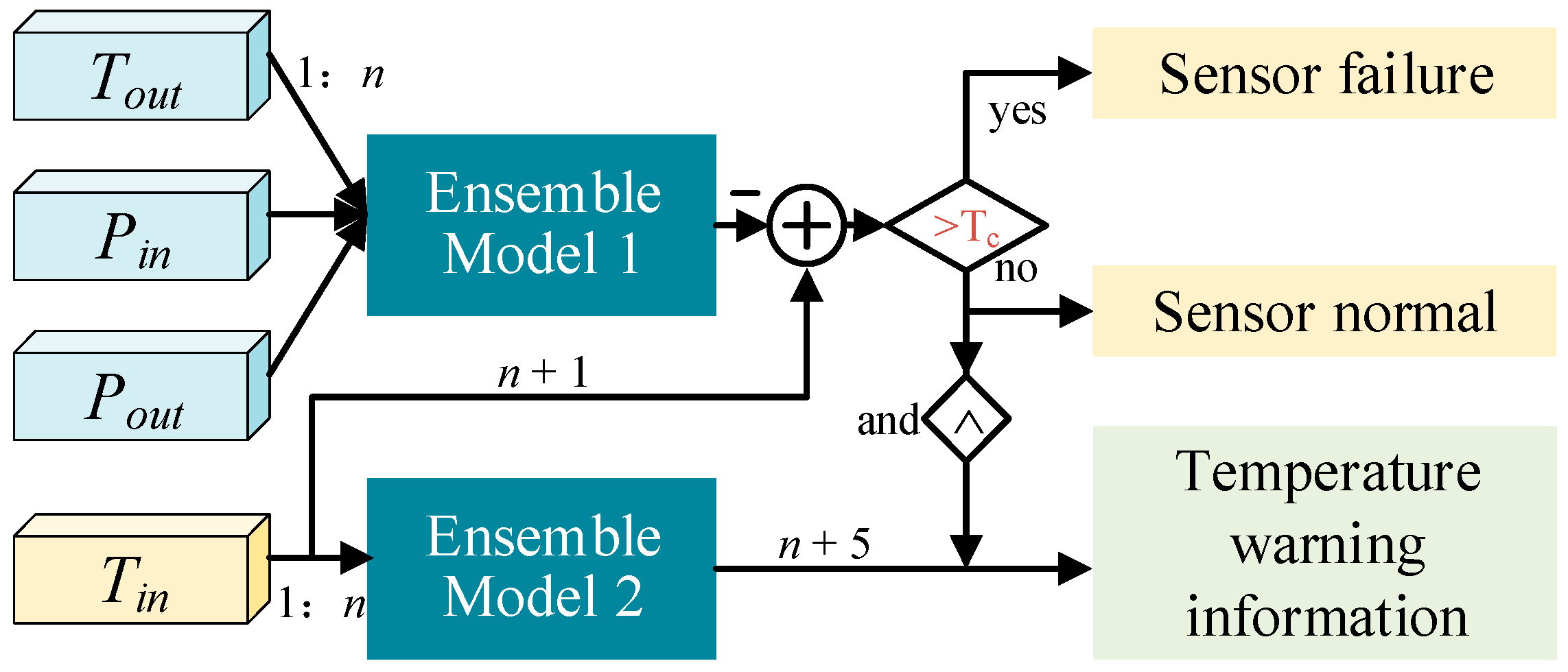
The proposed dual-level intelligent diagnostic architecture employs a cooperative ensemble prediction model to achieve coupled fault analysis in cooling systems, with its core operational mechanism illustrated in Figure 3 (model training details provided in Figure 4).

At the first level, Ensemble Prediction Model 1 integrates spatiotemporal correlation features extracted from multimodal sensor data (including outlet temperature, inlet pressure, and outlet pressure) to construct a dynamic prediction model under normal operating conditions. This model generates real-time physical parameter predictions for the n + 1 timestep. By comparing deviations between predicted and measured data against predefined thresholds, it achieves online sensor fault detection and signal isolation, effectively preventing interference from abnormal sensor data in subsequent diagnostics.

The second level implements Ensemble Prediction Model 2, which develops a machine learning predictor for inlet temperature time-series data. By capturing dynamic evolution patterns and periodic characteristics in historical sensor data, this model provides advanced temperature signal prediction, enabling early warning of abnormal conditions such as overheating.

The connection point between Integrated Prediction Model 1 and Integrated Prediction Model 2 represents a critical component of the overall process. When Integrated Prediction Model 1 verifies that the sensor is functioning within normal parameters by comparing the deviation against the predefined threshold T_C, the validated coolant inlet temperature data are forwarded to Integrated Prediction Model 2 as input. This ensures that only sensor data confirmed to be reliable under operational conditions are utilized in Model 2 for advanced temperature prediction and anomaly detection, thus preventing inaccurate predictions and false alarms that could arise due to sensor malfunctions.

This hierarchical dual-model architecture establishes a closed-loop verification mechanism through decoupling analysis of equipment-sensor parameters: It simultaneously validates individual sensor reliability via multi-parameter cooperative prediction while inversely deriving temperature information through single-parameter prediction. This approach overcomes the diagnostic bottleneck of coupled sensor distortion and equipment faults present in conventional methods, significantly enhancing the robustness and accuracy of fault diagnosis under complex operating conditions.

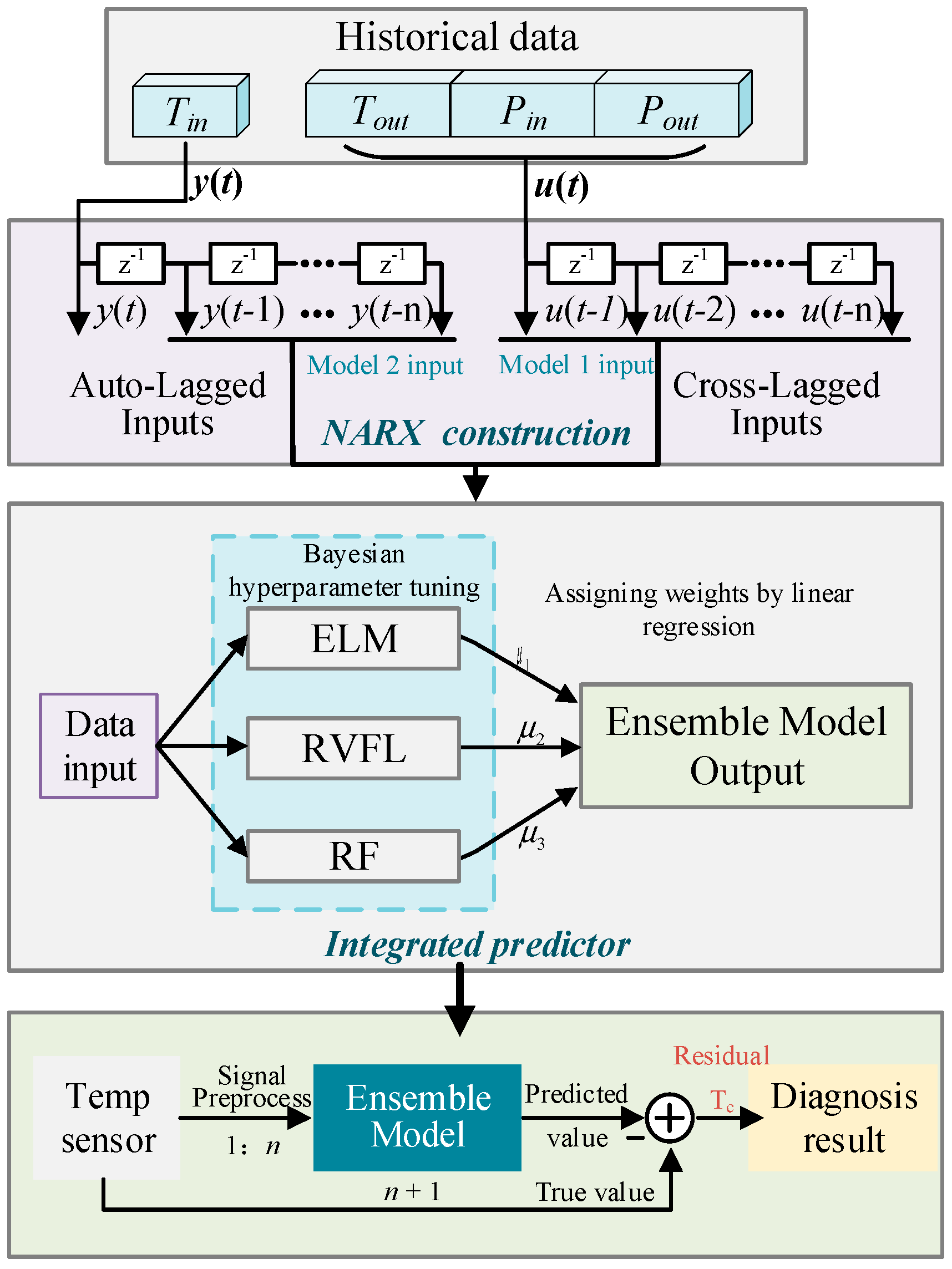
The proposed integrated predictor construction and fault diagnosis process, as illustrated in Figure 4, consists of three core technical components: data-driven modeling, multi-model fusion optimization, and residual-based diagnosis. During the model construction phase, the system first performs spatiotemporal feature reconstruction on historical data of cooling system parameters, including inlet temperature, outlet temperature, and pressure. By adopting a Nonlinear AutoRegressive with eXogenous inputs (NARX) model architecture, automatic lag processing is applied to the target variable y(t) to generate time-delayed sequences from y(t − 1) to y(t − n). Simultaneously, cross-lag processing is performed on correlated variables u(t) to create an input matrix spanning u(t − 1) to u(t − n), thereby capturing the dynamic coupling characteristics and temporal dependencies among system parameters.

During the training phase of the integrated predictor, a heterogeneous ensemble of base models was constructed, comprising the extreme learning machine (ELM), random vector functional link (RVFL) network, and random forest (RF) algorithm. This design leverages their complementary strengths: The ELM enables rapid computation via its single-hidden-layer architecture, the RVFL handles linear-nonlinear hybrid features through direct input-output linkages, and RF enhances robustness by employing bootstrap aggregation. Bayesian optimization performs a global search across the hyperparameter space of each base model to fully exploit their respective advantages—specifically, fine-tuning the hidden nodes of the ELM for speed–accuracy balance, optimizing the dimensionality of the RVFL’s enhanced layer, and calibrating the tree depth of RF to mitigate overfitting risks. A weighted fusion mechanism based on linear regression (with weighting coefficients ${\mu }_1$, ${\mu }_2$, ${\mu }_3$) dynamically integrates the outputs of multiple models.

In the fault diagnosis stage, historical sequences from temperature sensors are input into the trained ensemble model to generate predicted values for the n + 1 timestep. These predictions are then compared with actual measurements to compute residuals. If the residuals exceed the predefined threshold T_C the system triggers corresponding fault codes based on hierarchical diagnostic logic. This mechanism not only enables sensor anomaly detection through multi-parameter cooperative prediction but also facilitates inverter fault identification via single-parameter deep prediction inversion, thereby establishing a cross-verification closed-loop for equipment-sensor status monitoring.

3.2. Extreme Learning Machines

The ELM is an efficient machine learning algorithm based on the single-hidden layer feedforward neural network (SLFN), proposed by Professor Guang-Bin Huang [27]. This algorithm revolutionizes the traditional neural network training paradigm by randomly initializing hidden layer parameters and analytically determining output layer weights, significantly improving model training efficiency. The core concept of ELM lies in treating the hidden layer as a random feature mapping space and directly fitting outputs through linear regression, demonstrating broad application potential in classification, regression, and feature learning tasks.

The advantages of the ELM lie in its computational efficiency and theoretical completeness: The combination of randomly initialized hidden layer parameters and analytical solutions enables extremely fast training speeds, making it suitable for real-time applications; the global optimality of output weights avoids local optima issues inherent in gradient descent methods; and regularization and random feature mapping enhance generalization performance; while the algorithm remains compatible with diverse activation functions and task types. However, significant limitations are evident: Random initialization of hidden layer parameters may induce performance variability, necessitating multiple experimental trials to mitigate fluctuations; the hidden layer node count L relies on manual configuration, where excessive nodes risk overfitting and insufficient nodes lead to underfitting; the model exhibits sensitivity to data normalization; and the model’s single-hidden-layer structure hinders extension to deep networks while offering weaker theoretical interpretability.

3.3. Random Vector Functional Link

The RVFL represents an efficient learning algorithm based on single-hidden-layer feedforward neural networks [28]. Similar to the extreme learning machine (ELM), the RVFL significantly enhances training efficiency by randomly generating and fixing the weight matrix and bias vectors between the input and hidden layers, thereby eliminating iterative optimization processes. The calculation of the hidden layer output matrix $H=g(W^{T}X+b)$ aligns completely with that of the ELM.

However, the fundamental improvement of the RVFL lies in its feature augmentation mechanism: By concatenating the original input X with the hidden layer output H to form an augmented matrix $A=[X|H]\in {ℝ}^{n\times (d+L)}$, the model preserves both the linear components of input features and the nonlinear components of hidden layer mappings, thereby constructing a more robust feature representation space. The output weight matrix $\beta \in {ℝ}^{(d+L)\times m}$ is derived through the closed-form solution of regularized least squares:

$$\beta ={(A^{T}A+\lambda I)}^{-1}{A}^{T}Y$$

(4)

This formulation directly contrasts with the ELM, reflecting the RVFL’s innovative design that extends the regression basis from pure hidden-layer features H to a hybrid feature space A. This enhancement effectively mitigates the potential information loss in input features caused by the ELM’s complete reliance on random projections, demonstrating improved performance in scenarios with significant linear correlations between inputs and outputs. However, the increased dimensionality of the augmented matrix (d + L) introduces a marginal increase in computational complexity. For high-dimensional input features, overfitting risks must be suppressed through careful regularization coefficient λ adjustment. Despite these considerations, the RVFL retains the ELM’s core advantages of computational efficiency and global optimal solution characteristics, establishing itself as an ideal choice for small-to-medium-scale datasets requiring balanced linear and nonlinear modeling capabilities.

3.4. Random Forest

RF is an ensemble learning algorithm that enhances model generalization performance by constructing multiple decision trees and aggregating their prediction results [29]. The core mechanism of RF combines bootstrap aggregation (bagging) with random feature selection: First, multiple subsampled training sets are generated through with-replacement sampling, each used to train an individual decision tree. During node splitting, the algorithm randomly selects a subset of candidate features (typically the square root of the total feature count) from the complete feature set to increase inter-tree diversity and reduce overfitting risks. For regression tasks, optimal split points are determined by minimizing the mean squared error ($\mathrm{MSE}={\displaystyle \frac{1}{n}}{\displaystyle \sum _{i=1}^n{(y_i-{\widehat{y}}_i)}^2}$). After generating all decision trees, classification results are integrated through majority voting, while regression outputs are averaged.

The advantages of RF include high robustness (insensitivity to noise and outliers), overfitting resistance (achieved through bagging and random feature selection to suppress model variance), and quantifiable feature importance. However, it exhibits higher computational costs and weaker interpretability compared to single decision trees. This algorithm is widely applicable to high-dimensional data and complex classification/regression tasks, though caution is required regarding potential prediction biases in extreme noise scenarios.

4. Algorithm Validation

4.1. Data Acquisition

In the state monitoring of the traction inverter cooling system, an ensemble learning-based method was employed to predict the inlet temperature of the coolant. This method established time series models via two distinct operating modes, with all output results corresponding to the inlet temperature of the cooling water. In the first mode, Prediction Model 1 performs multivariate collaborative prediction by selecting system parameters such as cooling water outlet temperature T_out, cooling water inlet pressure P_in, and cooling water outlet pressure P_out that exhibit strong correlations with the cooling system’s inlet water temperature. Consequently, a multi-dimensional feature time series input is constructed. The feature dimensionality expands to N dimensions (N ≥ 2), enhancing the model’s adaptability to complex operating conditions by integrating cross-parameter dynamic coupling information. In the second mode, Prediction Model 2 adopts self-input prediction and directly constructs a univariate time series model using the historical data of the cooling water inlet temperature T_in. This approach segments the original continuously monitored temperature data into fixed time windows to characterize the temporal evolution patterns of the single temperature parameter.

The operational data originate from CR400 AF (developed by CRRC) EMU (electric multiple unit) runtime datasets provided by CRRC Academy, sampled at 5 Hz. The temperature and pressure data from the cooling system of the second traction inverter were selected and continuously recorded over a 100 min period. The structure of the dataset aligns with the specifications outlined in

Table 1. Cooling system data for CR400 AF trainsets.

Model	Data Types	Symbol	Unit
Model 2 input	Cooling water inlet temperature	Tin	°C
Model 1 input	Cooling water outlet temperature	Tout	°C
Model 1 input	Cooling water inlet pressure	Pin	kPa
Model 1 input	Cooling water outlet pressure	Pout	kPa

.

Following outlier treatment, the data undergo normalization and reconstruction using the NARX structure.

The specific parameter settings of Model 1 are as follows:

• Lagged exogenous input parameters: cooling water outlet temperature T_out, cooling water inlet pressure P_in, and cooling water outlet pressure P_out.
• Lag step size: n = 10, corresponding to a 2-s historical window (sampling frequency of 5 Hz).
• Prediction step size: k = 1, enabling real-time verification of sensor operational status.

For Model 2, the lag step size remains at 10, while the prediction step size k = 5 allows for a 1 s forward predictive horizon.

The selection of the lag step size n = 10 and the prediction horizon k = 5 is justified based on the following analyses:

• n = 10: Experimental evaluation of prediction performance across various lag step sizes (n = 5, 10, 15) demonstrated that n = 10—corresponding to a 2 s historical window at a sampling frequency of 5 Hz—effectively captures the dynamic behavior of the data while minimizing the risk of overfitting.
• k = 5: This setting satisfies the requirement for short-term prediction in real-world engineering applications, offering a forward-looking capability of 1 s, while maintaining acceptable prediction stability.

The processed dataset is partitioned into training, validation, and test sets in a 0.7:0.15:0.15 ratio.

4.2. Model Training

The proposed fault predictor employs a Bayesian-optimized heterogeneous ensemble architecture consisting of three core stages: base model optimization, dynamic weight integration, and residual-driven fault detection. Initially, three heterogeneous base models—the extreme learning machine (ELM), the random vector functional link (RVFL) network, and random forest (RF)—are constructed with customized hyperparameter search spaces. For the ELM, the optimization variables encompass hidden layer nodes (search range: 50–500) and activation functions (‘hardlim’, ‘sig’, and ‘sin’). RVFL optimization focuses on the regularization coefficient (log-uniform sampling range [10⁻², 10²]) and hidden layer nodes (50–500). RF hyperparameter tuning targets maximum tree depth (5–30) and tree quantity (50–500). The Bayesian optimization algorithm, leveraging a 5-fold cross-validation mean squared error objective function, conducts 200 optimization iterations on the training set to determine optimal hyperparameter configurations for each base model. The hyperparameter optimization process is visualized in Figure 5. The final optimal model training parameters are determined as follows:

■

ELM (extreme learning machine):

Hidden layer nodes: 158; activation function: ‘sin’.

■

RVFL (random vector functional link):

Activation function: ‘hardlim’; regularization coefficient: 2.53; hidden layer nodes: 103.

■

RF (random forest):

Maximum tree depth: 8; tree quantity: 466.

Subsequently, the prediction matrix $\widehat{Y}\in {ℝ}^{n\times 3}$ (where n denotes the number of samples) is generated from the base models using validation set data. The actual signal Y is the regression target, and the closed-form solution to solve for the weight coefficients with L2 regularization is

$$w={({\widehat{Y}}^T\widehat{Y}+\lambda I)}^{-1}{\widehat{Y}}^{T}y$$

(5)

The regularization coefficient λ is determined through the hold-out validation set to mitigate the negative impact of base model overfitting on ensemble performance. The final integrated prediction output is expressed as

$${\widehat{y}}_{ens}=\widehat{Y}w$$

(6)

The regularization coefficient λ was determined via grid search to be 0.4, and the weight coefficients of the linear regression model were optimized as [0.507, 0.375, 0.117].

As shown in

Table 2. Comparison of model prediction accuracy.

Data Model	RMSE	MAE	R2
Integrated Learning	0.0049	0.0027	0.8784
ELM	0.0056	0.0035	0.8415
RVFL	0.0062	0.0040	0.8056
RF	0.0088	0.0053	0.6086
LSTM	0.0094	0.0075	0.5653

, this study compares the root mean square error (RMSE) between the ensemble model and individual sub-models and also includes a comparison with the LSTM network. The results indicate that the prediction accuracy of the integrated model is significantly enhanced after introducing weight coefficients via linear regression optimization. The core strength of the integration method lies in its capacity to consistently improve the performance of diverse model architectures, thereby significantly reducing prediction errors. The experimental results further confirm that the weighted fusion integration strategy reduces the average RMSE across key baseline models—including RF, the RVFL, and the ELM—by 28.64%, with a minimum RMSE reduction of 12.5% observed for individual sub-models.

4.3. Offline Prediction Results

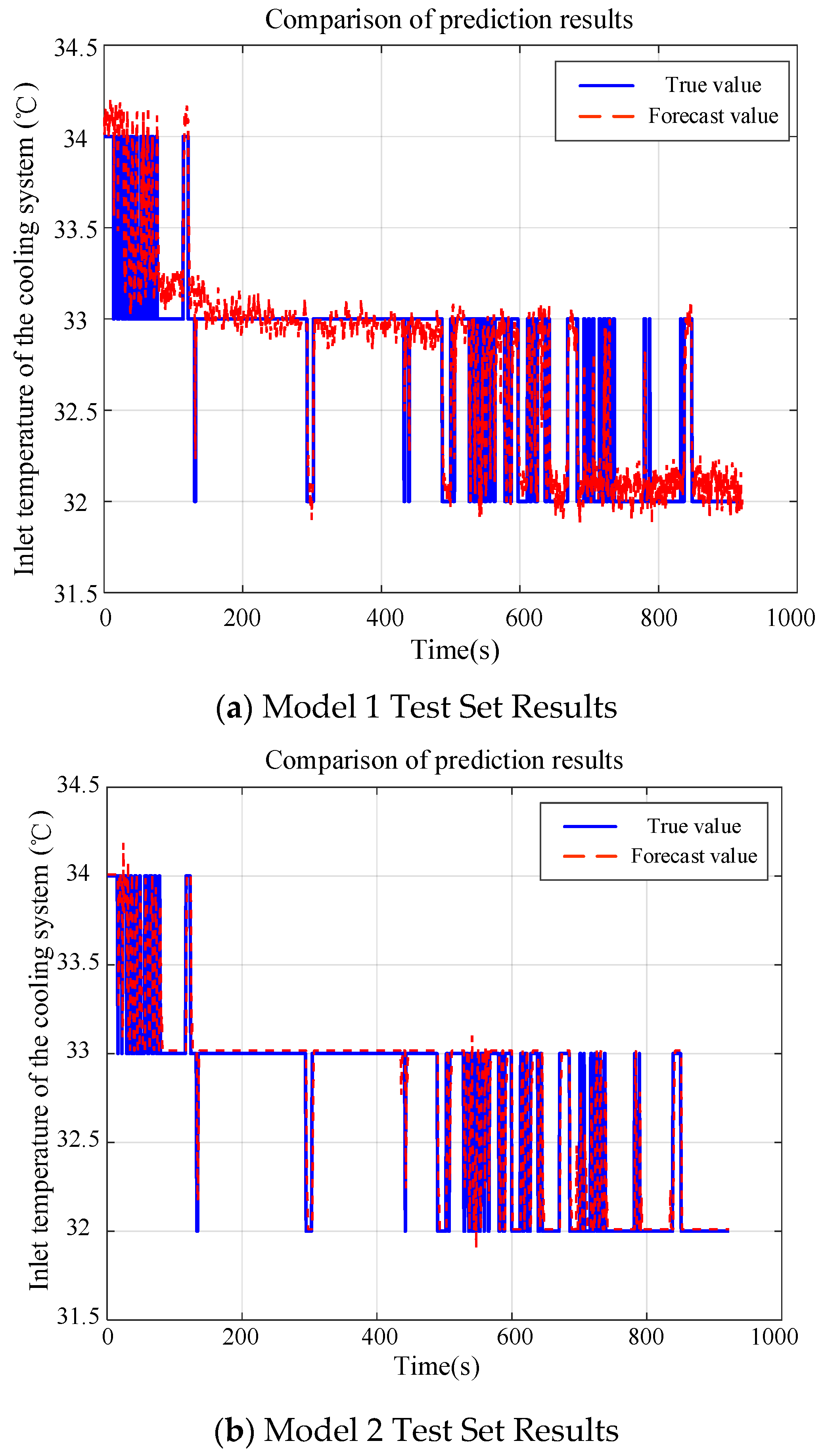
Figure 6a illustrates the dynamic prediction model established under normal operating conditions using Ensemble Prediction Model 1. This model incorporates n = 10 lagged sequences of cooling water outlet temperature T_out, cooling water inlet pressure P_in, and cooling water outlet pressure P_out to predict the physical parameters of the inlet temperature sensor at the (n + 1)th time step in real-time. The figure provides a visual comparison between the predicted results and the actual values. The model exhibits an RMSE value of 0.0049, indicating high predictive accuracy.

Figure 6b validates the time-series prediction capability of temperature sensor historical data by constructing a prediction model based on single historical temperature inputs. Sensor integrity is confirmed through first-level diagnostic verification. By utilizing n = 10 lagged sequences (equivalent to a 2 s historical window), the model achieves k = 5-step-ahead prediction (1 s) of temperature trends. Under normal operating conditions, the prediction curve shows high consistency with actual monitored values, and the model exhibits an RMSE value of 0.0056. The discrepancy between these parameters and the visual results can be primarily attributed to the root mean square error introduced by the time delay inherent in the predictor’s multi-step-ahead predictions. This analysis confirms that intelligent prediction based on historical temperature data can uncover underlying patterns in sensor data and decouple the coupled characteristics between equipment anomalies and sensor faults, thereby providing proactive decision-making support for converter health management when sensor reliability is assured.

During the fault detection phase, real-time residual sequences are computed as follows:

$$e_t=|y_t-{\widehat{y}}_{ens,t}|$$

(7)

Dynamic thresholds are set by fitting residual distributions based on historical normal data:

$$\tau ={\mu }_e+3{\sigma }_e$$

(8)

where ${\mu }_e$ and ${\sigma }_e$ represent the residual mean and standard deviation, respectively. If the residual difference between the predicted result and the true value exceeds the threshold, it indicates the occurrence of a fault. Furthermore, ${\mu }_e$ and ${\sigma }_e$ are dynamically updated based on real-time operational conditions, ensuring that the system adapts to the current system state and minimizes false alarms while maintaining sensitivity to faults.

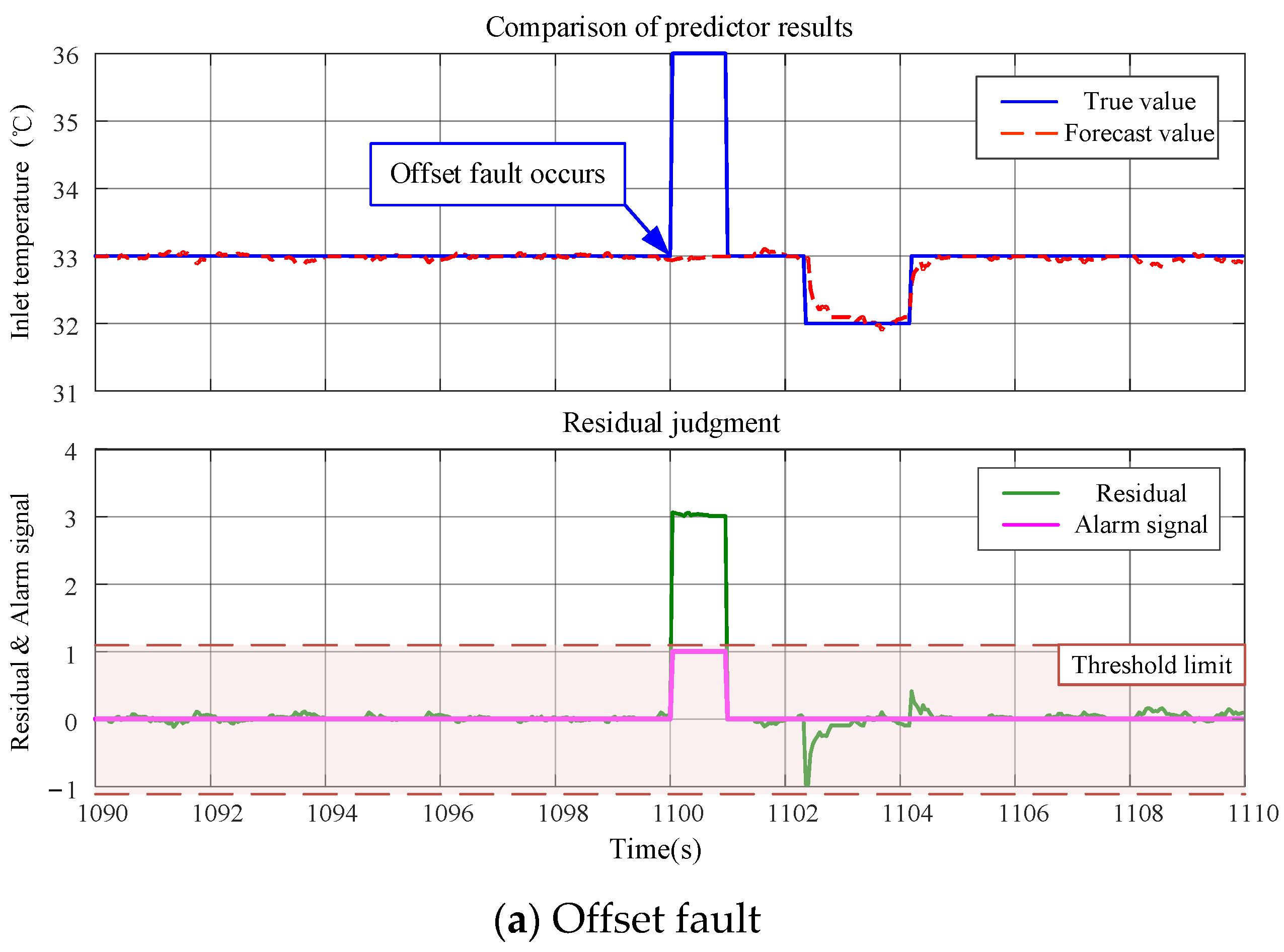
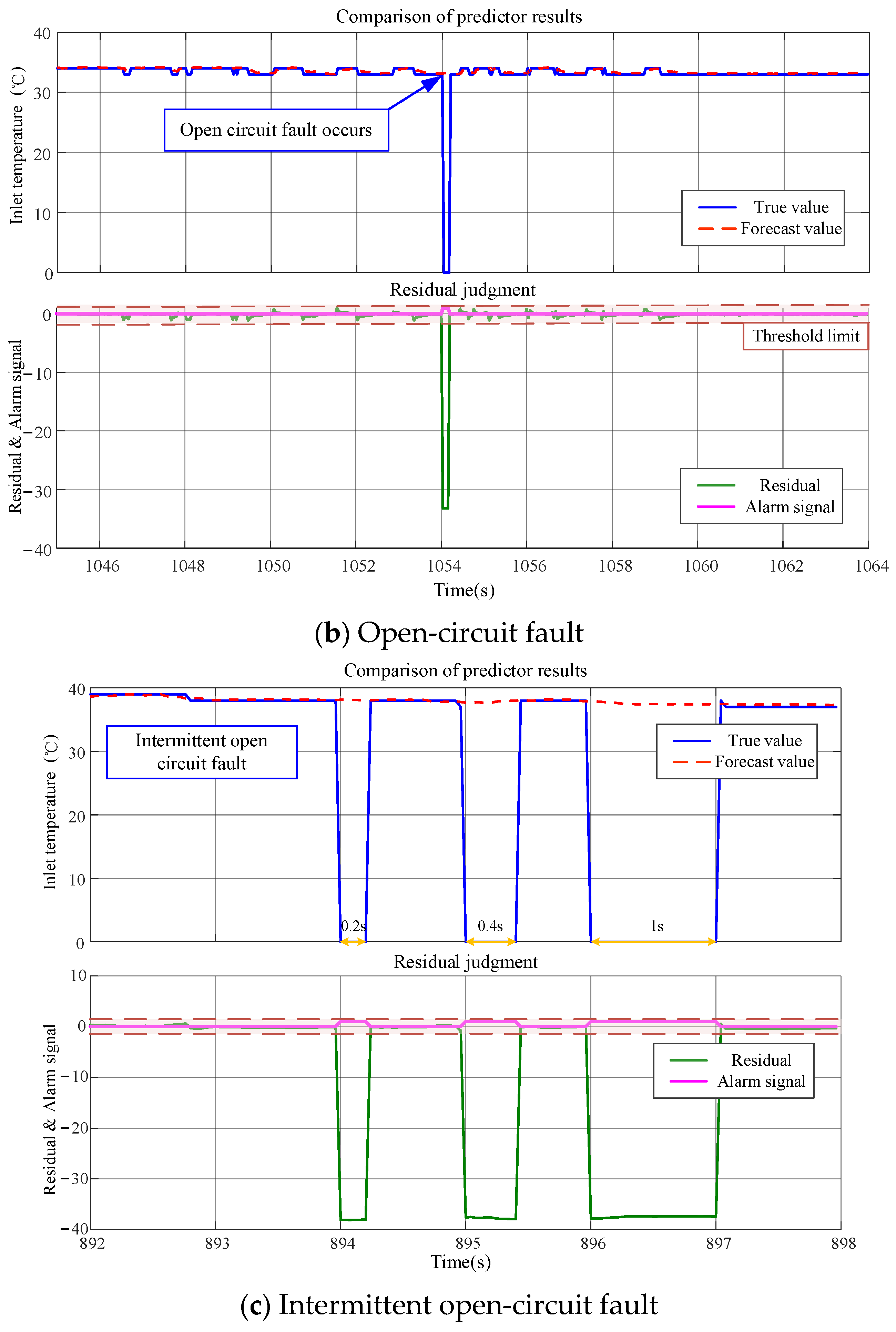
Figure 7 presents the MATLAB R2023b/Simulink simulation results of the cooling system’s operational dynamics. The three subplots are configured with identical dual-panel structures: The upper panel contrasts Predictor 1 outputs with ground-truth measurements, while the lower panel visualizes residual sequences alongside dynamically determined threshold boundaries. An alarm protocol is automatically activated when residuals exceed established thresholds, thereby validating the detection capability for abnormalities in the inlet temperature sensor.

Diagnostic scenarios for offset and open-circuit faults are illustrated in Figure 7a and b. The verification process was further extended through diagnostic testing for intermittent open-circuit faults, as illustrated in subfigure c, to enhance model robustness and practical applicability. Three operational scenarios were systematically simulated at a 5 Hz sampling rate, featuring fault durations of 0.2 s, 0.4 s, and 1 s, respectively. This progressive fault duration scheme accurately replicates the transient characteristics of real-world intermittent faults. A significant discrepancy between predicted and actual signals emerges during cooling system inlet temperature sensor failures, attributable to the predictor’s incorporation of correlated signal inputs. Subsequent threshold-based evaluation triggers immediate alarm signal activation, conclusively demonstrating the methodological effectiveness.

4.4. Online Validation Results

To validate the engineering deployment capability and real-time performance of intelligent algorithms on embedded edge devices, this study establishes an experimental platform for predicting the temperature of a traction converter cooling system based on the NVIDIA Jetson Orin NX. The edge computing system features a compact modular design and utilizes network interface communication to achieve low-latency data exchange. Benchmarking results confirm that under typical operating loads, the system achieves an average inference latency of 10 milliseconds for Ensemble Prediction Model 1 while the sampling period of the sensor is 200 milliseconds. These metrics demonstrate the system’s ability to meet the millisecond-level real-time processing requirements of complex algorithms. The platform architecture consists of the following core modules:

• Edge Computing Unit: executes temperature prediction algorithms to process sensor time-series data in real time.
• Operating Condition Simulator: generates real-time sensor output data to simulate the dynamic behavior of a traction converter cooling system under both normal and predefined fault conditions (e.g., sensor bias, drift, or complete failure).
• Communication Relay: establishes deterministic, low-latency network transmission channels between devices.
• Verification Terminal: conducts closed-loop validation by comparing predicted values against the simulator-generated “ground truth” data through a visual interface.

The platform operates in three sequential phases: First, the operating condition simulator generates real-time cooling system data, which are transmitted via Ethernet to the edge computing unit. Next, the prediction model extracts spatiotemporal features and analyzes temporal correlations from the incoming temperature data stream to generate predictions for future time windows. Finally, the prediction results are returned to the simulator, and both the predicted curves and the simulator’s output are displayed synchronously on the verification terminal for performance evaluation. 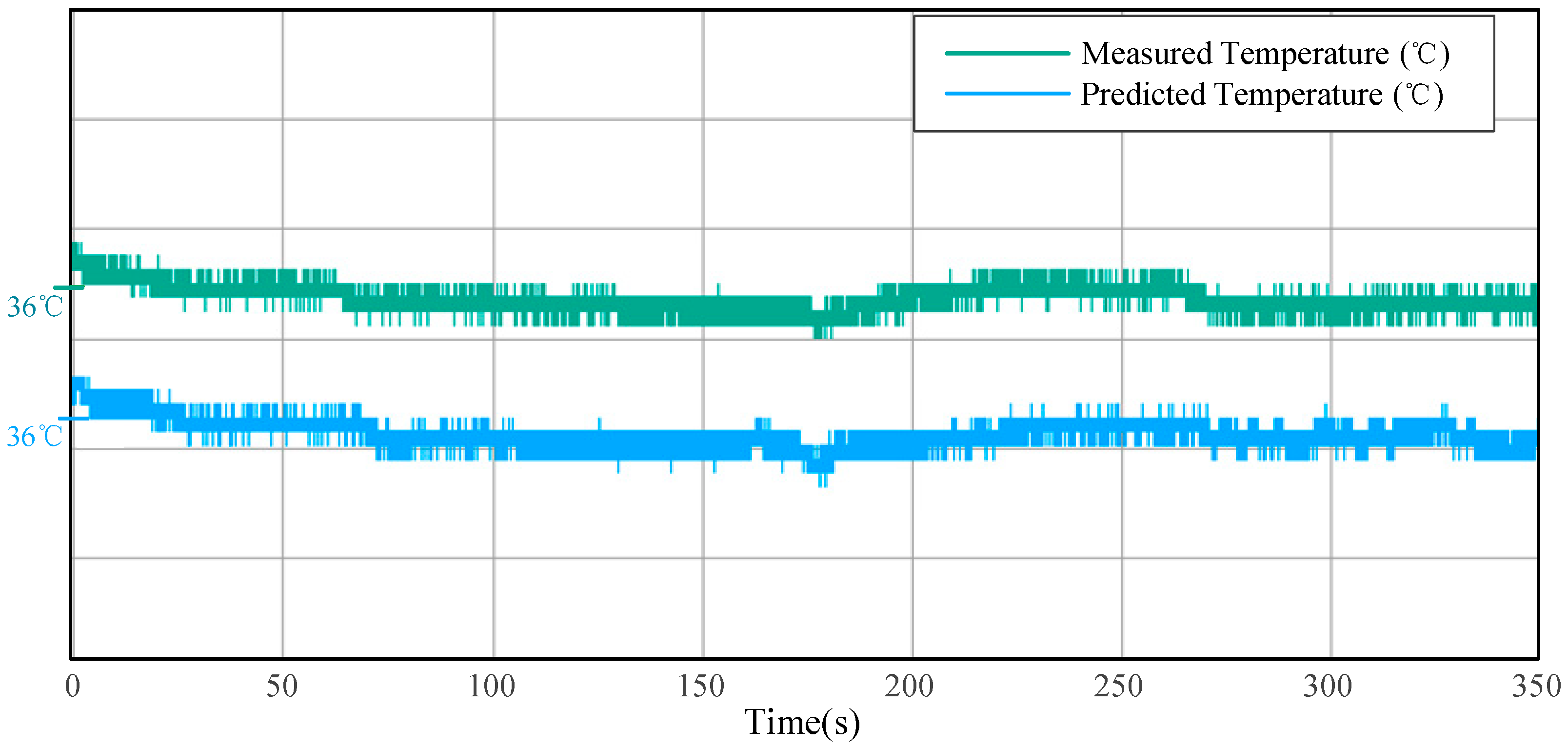Figure 8 illustrates the prediction model’s output fidelity under normal conditions, while Figure 7 presents comprehensive fault detection results using residual analysis and thresholding.

Figure 8 demonstrates the output accuracy of the predictive model (Ensemble Prediction Model 2) running on the edge platform under simulated normal operating conditions. The predicted inlet temperature (prediction value) derived from the model and its corresponding “true value” (simulation value) are displayed in this figure. To improve waveform visibility, the two signals are vertically separated and annotated with their respective 36 °C reference points for amplitude comparison, with both waveforms scaled at 5 °C per grid division. The model’s capability to accurately track the system dynamics in real time on the edge computing platform has been experimentally validated.

4.5. Robustness Verification

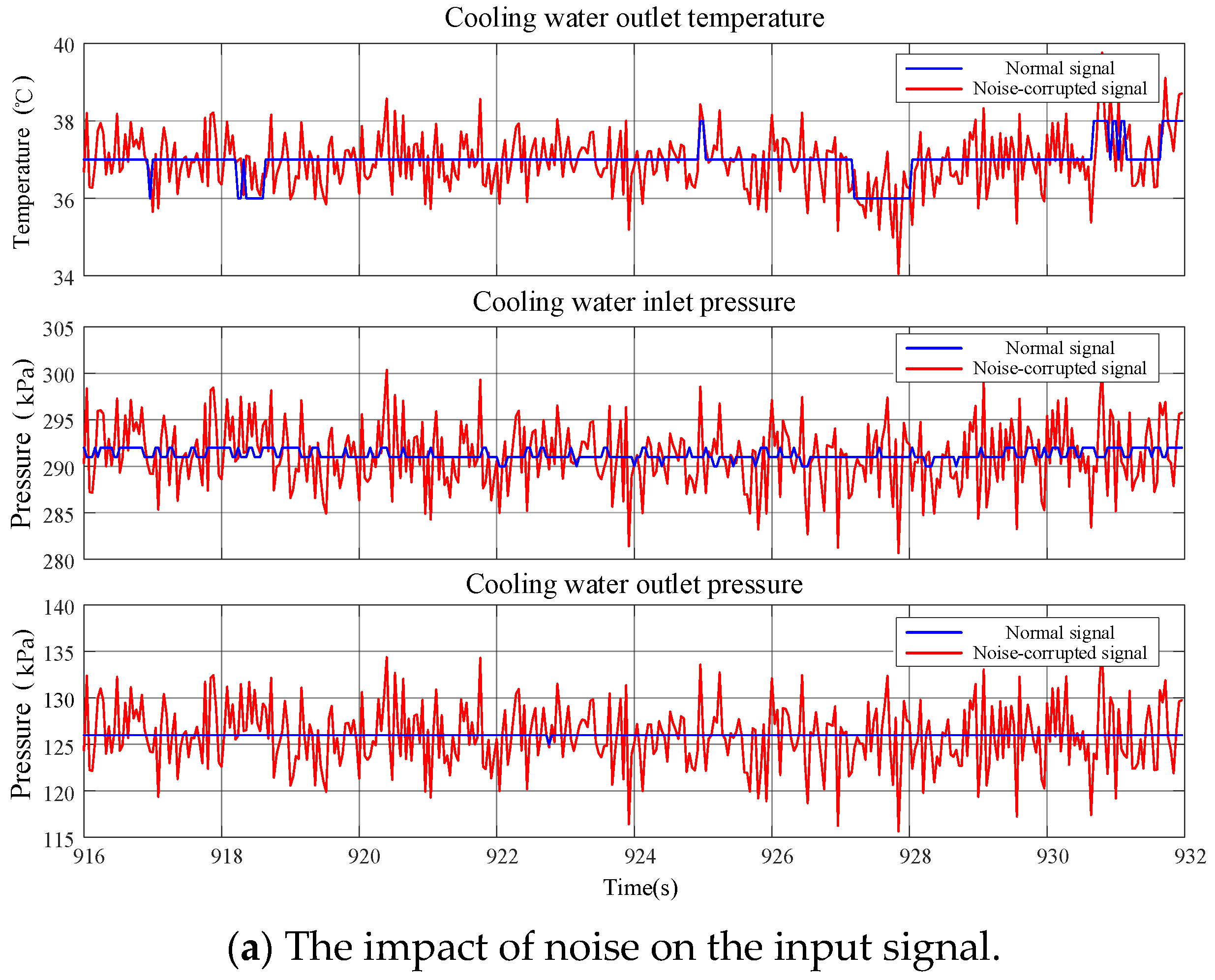
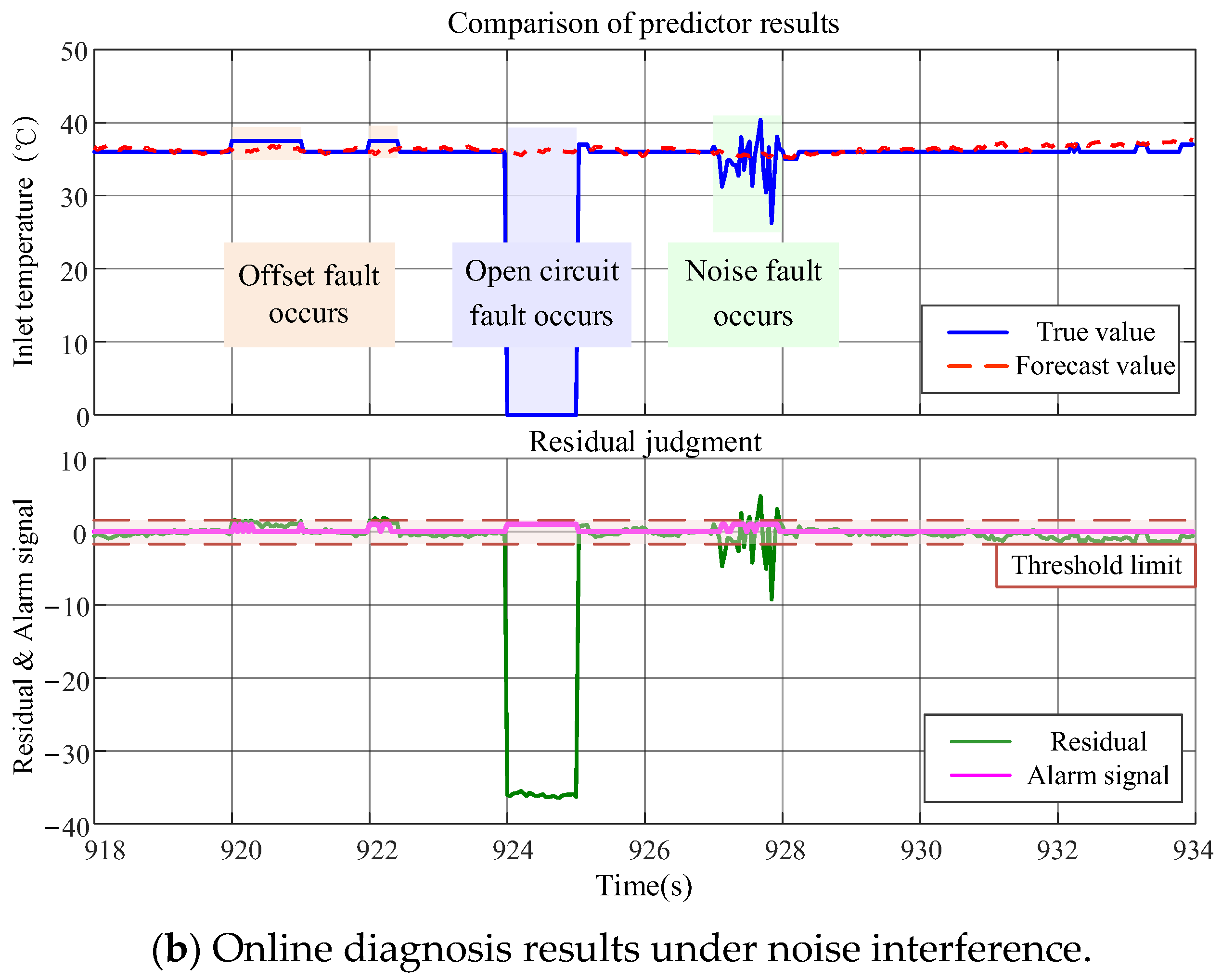
The prediction performance of Predictor 1 under 5% noise interference in the input signal is presented in Figure 9, with diagnostic results for offset, open-circuit, and noise-induced faults simultaneously demonstrated. It should be noted that due to the predictor’s lag step size (n = 10), a 2 s temporal offset was introduced between the two subplots in Figure R5-2 to ensure the proper alignment of input and output sequences. A comparative analysis of input signals before and after noise injection is demonstrated in Subplot (a), quantitatively characterizing the noise contamination level. Subplot (b) exhibits the model’s predictive outputs and fault diagnosis outcomes under noisy conditions. Although the presence of noise was observed to slightly degrade prediction accuracy, the majority of faults were effectively identified through the threshold-based diagnostic mechanism. These experimental results confirm that significant predictive and diagnostic capabilities are retained by the model under noisy input conditions, thereby validating its robustness.

Operational data from the traction cooling system of a different train unit are employed for external validation of data source independence, as shown in Figure 10. As illustrated in Figure 10a, when the pre-trained Predictor 1 is directly applied to the independent dataset, the overall temperature trend is successfully captured; however, a discrepancy of approximately 2 °C between predicted and actual values is observed due to differences in data ranges across trains, resulting in an RMSE of 0.0491. To address this issue, 20% of the dataset is reserved as an independent validation set for weight re-calibration, yielding optimized weights of [0.087, 0.574, and 0.292]. The improved prediction outcomes, with an RMSE significantly reduced to 0.0116, are presented in Figure 10b. These findings confirm that the proposed ensemble learning model can effectively predict temperature trends; however, performance may be affected when test data fall outside the training range. Importantly, the improvement achieved through weight re-adjustment highlights the efficacy of the weighting mechanism in mitigating discrepancies caused by data range variations.

5. Conclusions

This study presents a collaborative diagnostic framework based on a dual-layer intelligent architecture, designed to address the complex coupling between temperature sensor faults and equipment failures in traction inverter cooling systems. By integrating spatiotemporal features extracted from multimodal sensor data through an ensemble learning model, the proposed method enables the rapid identification of inlet temperature sensor faults and accurate prediction of the thermal behavior of the inverter cooling system. The robustness of the model has been systematically evaluated and validated within this study. The experimental results demonstrate that the model is capable of handling noisy environments; however, its predictive accuracy decreases when tested on data outside the training distribution. Future work will aim to improve the model’s generalization across diverse data sources through algorithmic optimization and will emphasize real-time validation under practical operational conditions.