Abstract
Navigation technologies are becoming more advanced, helping to solve complicated problems in various fields. Navigation can be classified as global, in which predefined data and reference points from the working environment are used to generate a path, and local, where the map is generated momentarily by acquiring data from outside using sensors. As navigation tasks become more demanding, working environments can become very complicated with an increasing number of dynamic obstacles or, in some cases, a lack of global references, which may have particularly notable impacts on communication. Inspection robots that are required to work in underground sewers are often required to work completely locally, relying on sensor data. For this reason, in this study, a cost-efficient laser marker-based obstacle detection and measurement system is designed and tested for future use in autonomous sewer robot local path generation. Our experiments show the convenience of applying four linear laser markers with an RGB camera to fully inspect upcoming obstacles in the region covering the front robot dimensions. The results show distance measurement accuracy of up to ±1.33 mm and obstacle width accuracy of up to ±0.28 mm measured from a 130 mm range. Nevertheless, accuracy is strongly dependent on the segmentation of image resolution, lighting, and reflection of the inspected surfaces. Also, it depends on the configuration of laser markers and the RGB camera position.
1. Introduction
Navigation technologies are advancing rapidly with the adoption of sensor fusion and artificial intelligence (AI). Recent advances in AI are paving the way for autonomous systems. However, as technologies advance, tasks are also becoming increasingly complex.
Navigation can be categorized as global or local. Global navigation involves relying on predefined information about the working environment, which can contain marked tracks, labels, and global communication systems. In this case, the optimal path to the target is generated in advance [1,2]. On the other hand, local navigation relies on sensor data to acquire information from the environment and momentarily make a decision about which direction to move in [3,4]. Nowadays, even systems that are integrated in a well-prepared environment, like automated warehouses, cannot fully rely on global information. One of the reasons for this is that various dynamic obstacles can introduce unpredictable obstructions [5,6]. Furthermore, for inspection-type robots that work in places that are difficult for humans to reach, the robots often need to completely rely on local sensor data [7,8]. Such environments also involve underground sewers, which require regular checkups, and performing such checks physically by hand can cost a lot or may be completely impossible. For this reason, a fully autonomous mobile sewer robot is being designed.
An essential step for navigation system development is localization. Local navigation sensors for measuring distance are of utmost importance for mobile robots. Optical sensors are very popular due to their high accuracy and fast response time, including time-of-flight (ToF) sensors, which evaluate distance by measuring the amount of time it takes for light to travel from the source and return from a reflective surface [9]. However, they are usually designed for one-point measurements and require a multiple-sensor solution for wider field-of-view capability. LiDAR sensors are another alternative that often have integrated drives for rotation and point cloud measurement in the 2D plane or even 3D space [10,11,12]. These sensors provide a wide measurement range and accuracy. On the other hand, optical sensors are sensitive to lighting and weather conditions. In this case, Radar sensors have an advantage, but at the cost of precise point cloud mapping [13,14,15].
To maximize localization, different sensors are fused together to compensate for their limitations. Distance sensors are often mapped with cameras to expand the amount of information received from the environment for better interpretation of detected objects [16]. Some of the cameras that are widely used for mobile robot navigation include RGB cameras used for color recognition. By mapping color data with distance sensor data, accurate estimation can be made about detected objects’ shape, geometry, type, and other characteristics [17,18]. Cameras can also be categorized into 2D cameras, which convert data to a plane from a specific field of view varying from 40° to 360°, including fish-eye cameras, or 3D cameras, which also include depth data. These cameras work by integrating ToF or LiDAR sensors or using several integrated cameras, like stereo cameras [19,20,21]. Another alternative, which is more robust to environmental conditions, is ultrasonic sensors, which are cost-efficient and accurate for short-range measurement [22,23].
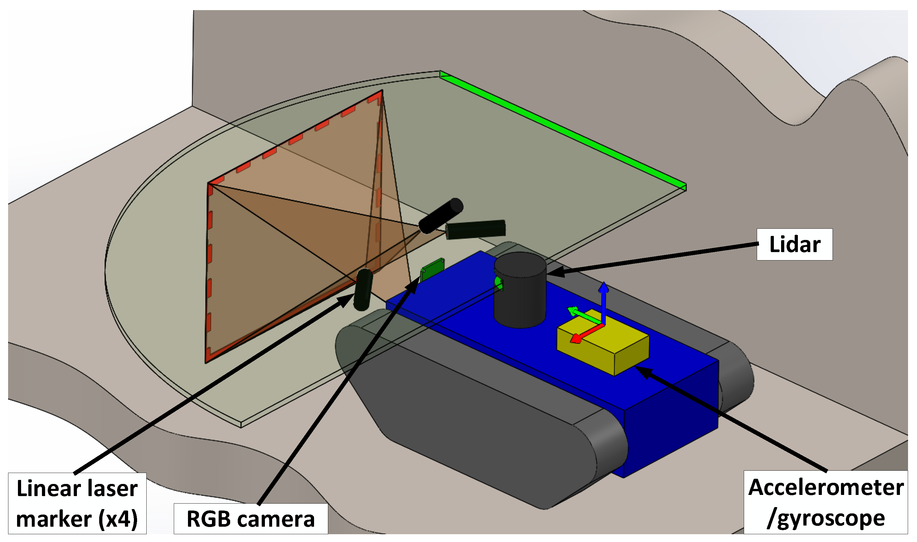
An RGB camera was selected for designing an autonomous sewer robot localization. In combination with four linear laser pointers, depth information can be received from the environment, thus creating an accurate, robust, and cost-efficient object detection solution, which is the main criterion for this system. In the literature, similar methods were experimentally analyzed. In [24,25], one linear laser marker is applied in combination with an RGB camera to detect and measure the distance from an obstacle. On the other hand, this combination only allows inspection of one surface or obstacles attached to the ground. Using two linear laser markers, as described in [26], allows for better surface scanning, minimizing blind spots. Nevertheless, in a sewer-like environment, obstacles can hang from the ceiling or walls. Four laser pointers covering the main planes allow for an optimal field of view, saving the computational resources required for image processing. The proposed laser scanner configuration is shown in the principal scheme of the developed sewer robot system presented in Figure 1.
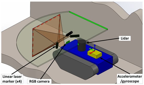
Figure 1.
Principal scheme of an autonomous sewer robot.
The red lines represent the possible detection field of view marked by linear laser pointers. To further extend the robot’s field of view, 2D LiDAR is added to better recognize the sides of the robot, which comes in handy in close gaps. In addition to object recognition, odometry data are also important for local navigation systems. Some of the sensors most frequently used for this purpose are accelerometers and gyroscopes. An accelerometer is very useful for measuring tilt, which is important in challenging terrain scenarios, while a gyroscope helps to check the robot’s rotation [21,27,28]. Both of these sensors are integrated into the designed robot system for better orientation. Magnetometers are also very useful for estimating heading, which is commonly combined with accelerometers and gyroscopes, but due to their dependency on the magnetic field, it is not reliable for underground sewer conditions [29].
In this work, the effectiveness of the designed laser scanner is analyzed. In the first part, the methodology of laser triangulation principles and adaptation for the designed laser scanner is discussed. Then, the working method of object detection is analyzed, and is further used for experimentation. Moreover, the experimental setup for determining object recognition accuracy is explained, including the chosen equipment, calibration of the system, and image processing. After that, the results of the experiments are presented, and the standard deviations of measuring different obstacles with different image segmentations are evaluated. Finally, conclusions are drawn and future works are discussed.
2. Materials and Methods
As previously mentioned, an autonomous robot for underground sewers requires a reliable and computationally cost-efficient solution for object detection. One of the most versatile devices for object recognition is an RGB camera. Nevertheless, to simplify the amount of information gathered from images, it is important to simplify the task as much as possible and search for specific patterns. In this case, laser pointers are used to provide linear contours that can be recognized from an image and interpreted for obstacle detection purposes. This reduces the amount of information required to process compared to depth camera point cloud data. Further experiments are performed to estimate the accuracy of the designed laser scanner distance measurement system.
2.1. Laser Scanner Obstacle Detection System Configuration
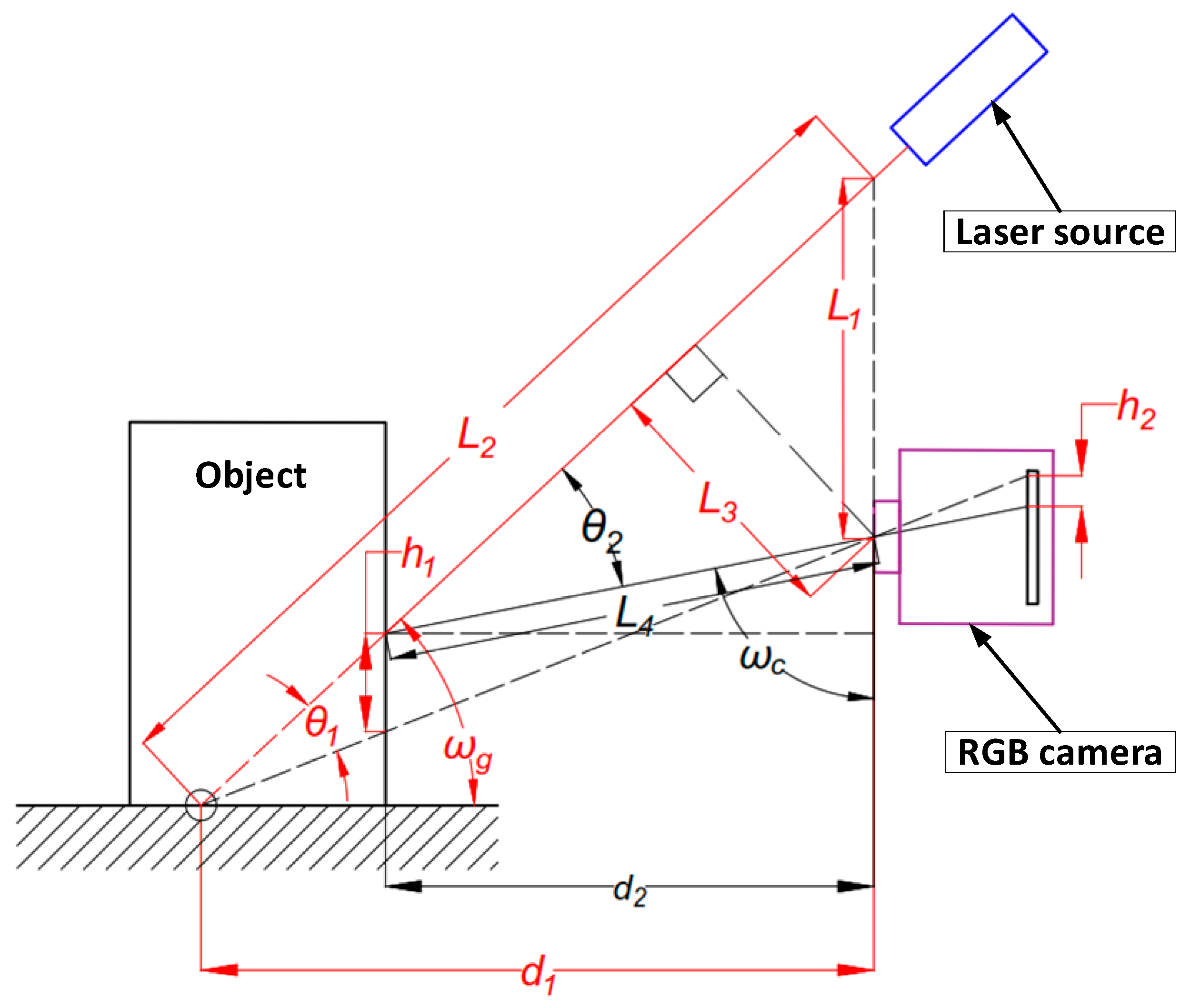
As previously mentioned, a combination of an RGB camera and a laser pointer has been researched in the literature as a practical obstacle detection, distance, and geometry measurement solution. The main idea behind this method is laser triangulation, as shown in Figure 2.
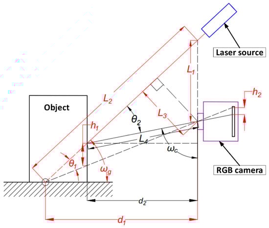
Figure 2.
Configuration of one linear laser pointer based on triangulation principles.
The obstacle obstructs laser light, which is reflected from the surface of an obstacle, resulting in displacement h1 from the laser reflection on the ground. Displacement h1 is then projected onto the CCD sensor, resulting in displacement h2, which is processed and scaled on the image by the RGB camera. To calculate the distance from the obstacle d2, additional parameters are needed, which are configured initially for the designed system. For this project, the system is configured by fixing the focus distance—d1, the linear laser tilt angle—θ1, and the camera perspective to the focus point tilt angle—ωg. The following formulas are used to detect the actual distance:
Then, the obstacle is present along the measuring range equal to d1. The distance from an object can also be defined by two resulting angles tilted from laser and camera projections, respectively—θ2 and ωc. Tilt angles for a specific distance can be found using the following formulas:
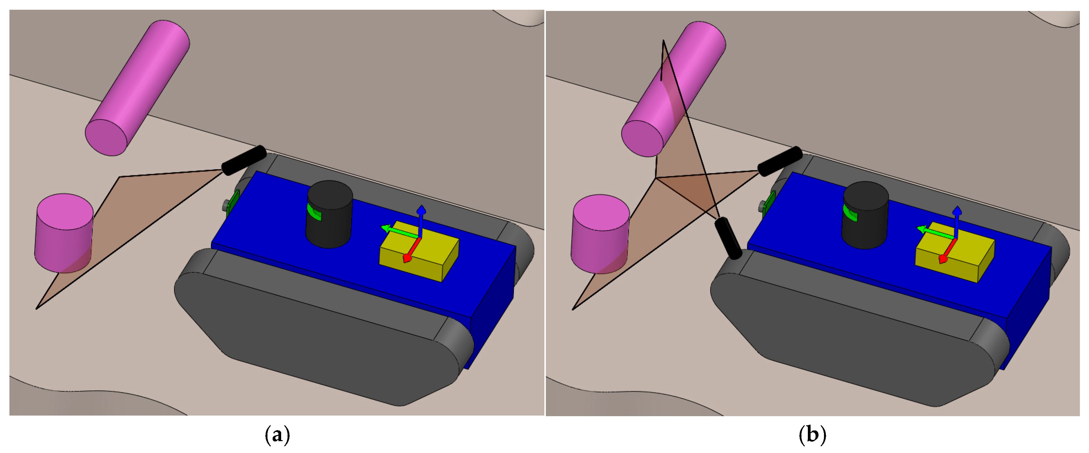
These formulas are further used for camera input data post-processing to create a map of occupied regions, later used for path planning. Nevertheless, one linear laser pointer is not enough to recognize all obstacles in front of the robot covering d1 range. In Figure 3a, it can be seen that the upper linear laser is able to mark only the obstacle from the left, which is fixed to the ground. This could lead the robot to move right and collide with an obstacle fixed to the wall.
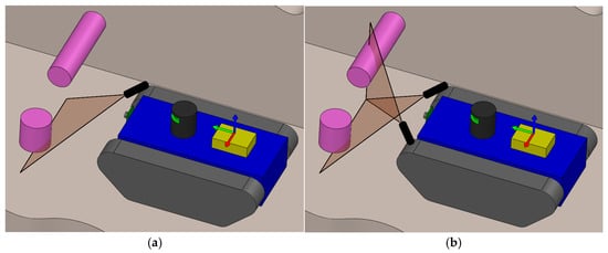
Figure 3.
Obstacle recognition with mobile robot (obstacles marked in purple and laser linear projections in red): (a) obstacle detection with one laser pointer; (b) obstacle detection with two laser pointers.
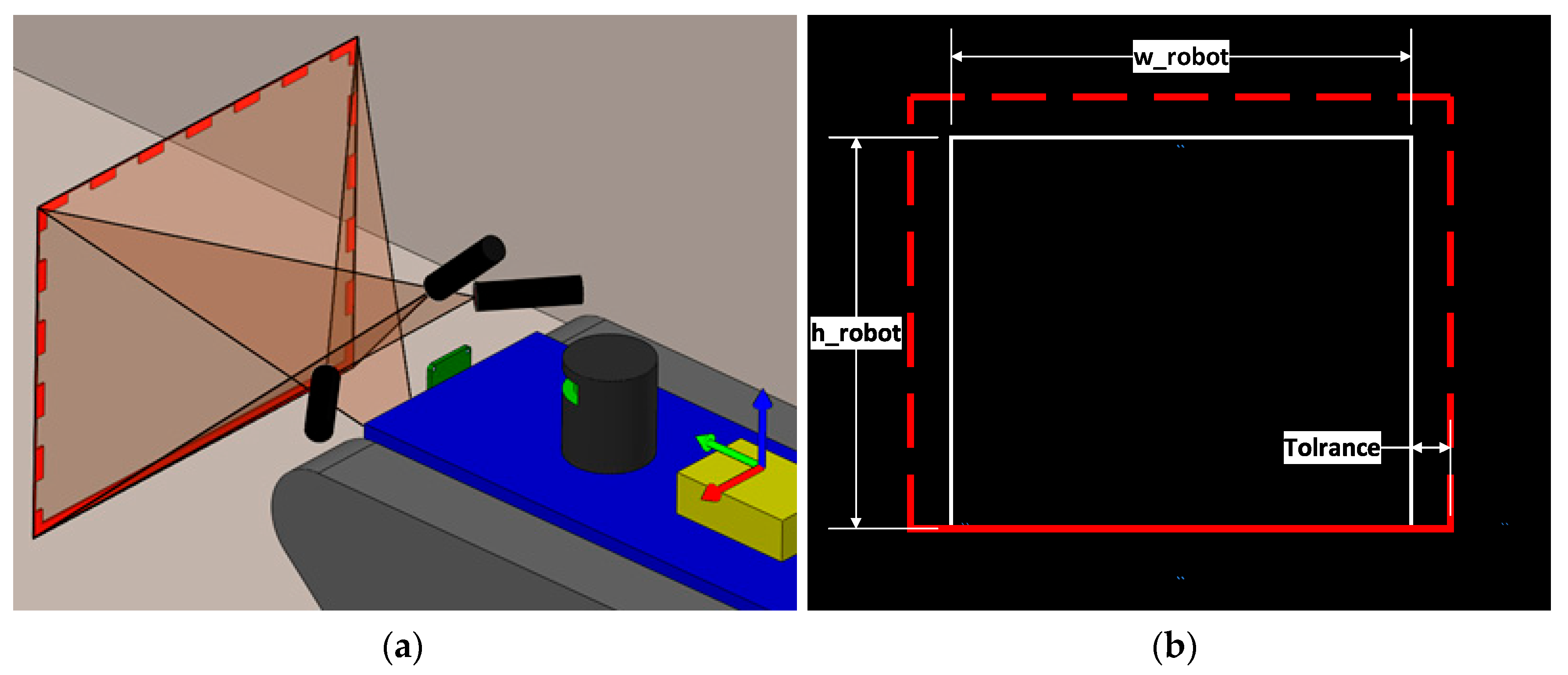
Adding another laser marker pointing from the left side allows us to detect the obstacles fixed to the right wall, as shown in Figure 3b. Moreover, adding laser markers from the bottom and right sides allows for the detection of obstacles fixed to all surfaces, creating a field of view whose size depends on the system configuration, linking each laser marker with the camera, as shown in Figure 2. Thus, the rectangular field of view is created by adding additional tolerance around the dimensions of the robot, as shown in Figure 4b.
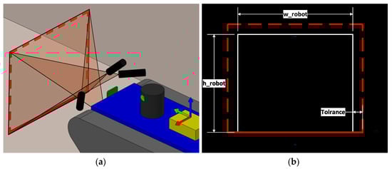
Figure 4.
Laser scanner field of view using four linear laser markers (laser linear projections marked in red): (a) side view of laser scanner field of view; (b) front plane of laser scanner field of view.
In Figure 4b, it can be seen that tolerance is added around the dimensions of the front robot projection. As a laser scanner is used as the main detection method for nearest obstacles, additional tolerance is necessary for detecting incoming obstacles. In Figure 4a, a laser scanner view from the side can also be seen, each projection marking a different plane in the rectangular tunnel.
2.2. Laser Scanner Experimental Setup
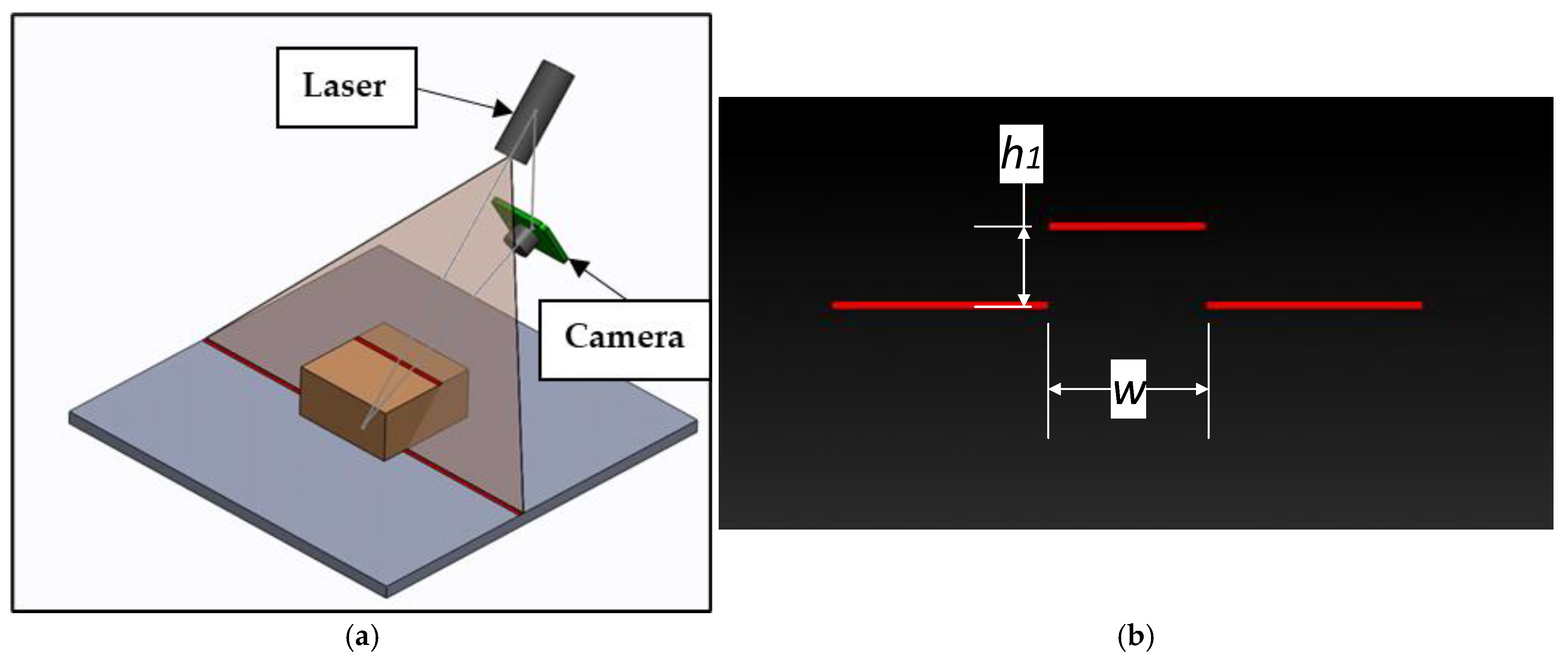
To test the designed scanner, the first experiment will be performed with one laser pointer. The goal of this experiment is to check the accuracy of distance measurement to an obstacle using an RGB camera and a linear laser marker. Accuracy is estimated by comparing the measured value with a laser scanner and the real dimensions. The laser that projects the light to the ground is used as shown in the simplified configuration of the system in Figure 4a.
In Figure 5b, a camera view example is shown corresponding to the position of the measurement system in Figure 5a. From an image, not only can displacement—h1—be measured, as explained earlier, but width—w—can also be measured, and the result can be directly converted to the real width of an obstacle. During the experiment, only cuboid forms are used as obstacles for testing the system. To be able to evaluate the accuracy of the designed measurement system, it is important to gather relevant data. For this reason, obstacles of different widths are used, including obstacles that are 5, 10, 30, and 50 mm wide. During the experiment, an obstacle is put in front of the laser scanner in a tunnel-like environment, as shown in Figure 6.
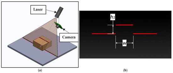
Figure 5.
Experiment principal scheme—laser scanner with one laser marker (laser marker linear projection marked in red): (a) 3D view of the system; (b) camera view of laser scanner when an obstacle is present.
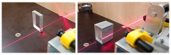
Figure 6.
Distance and obstacle width measurement using laser scanner in a tunnel-like environment.
The object is also centered on the camera. Initially, it is placed 130 mm from the scanner, which is the measuring range of the camera—d1. After that, the laser scanner is moved to an obstacle in increments of 5 mm up to 50 mm. The image is taken and processed at each increment. This procedure is performed with all four obstacles of different widths and additional changes in the image processing segmentation parameter, which will be discussed further.
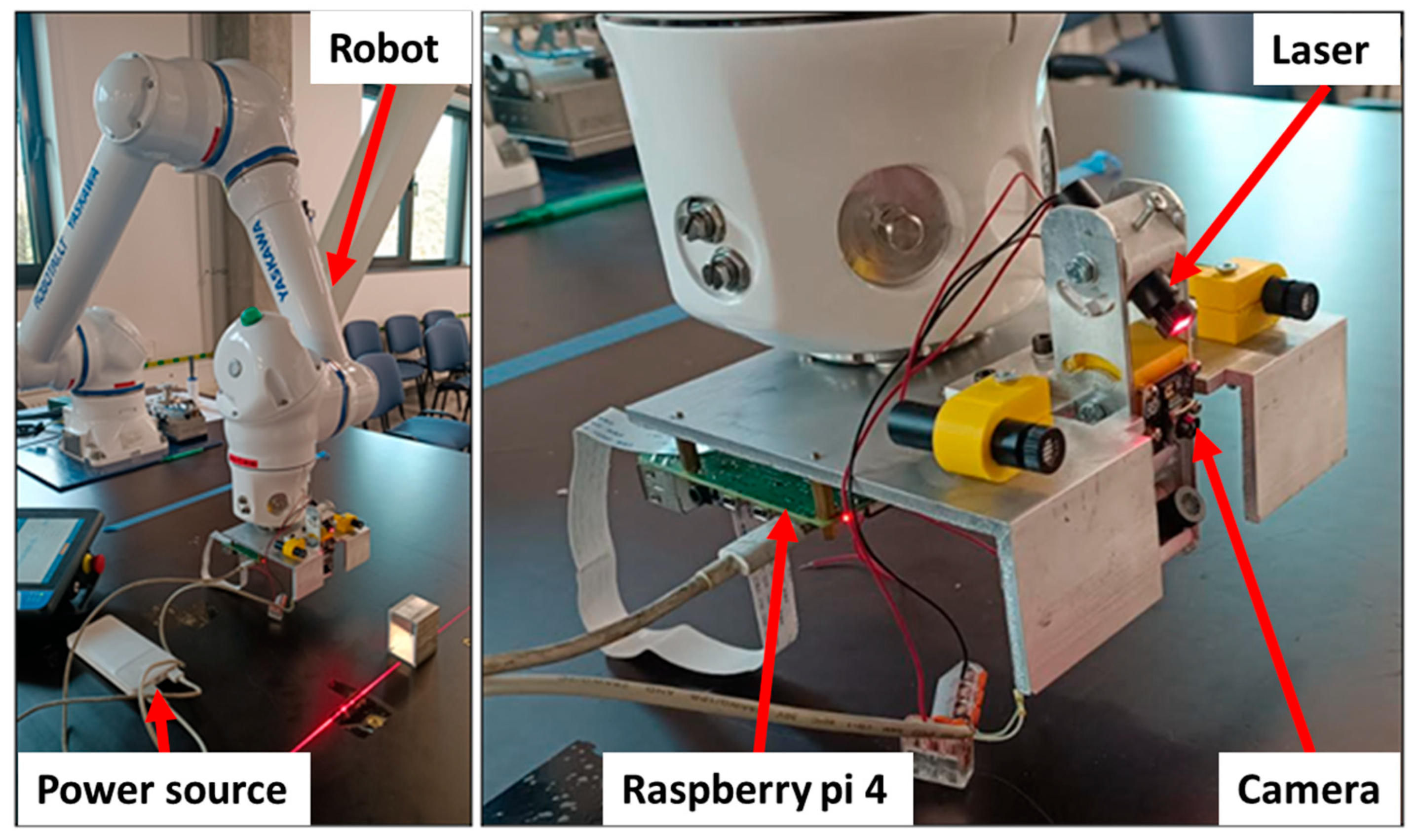
For this experiment, a measuring system prototype was created according to the geometrical specifications of the mobile sewer robot, which is in development. The prototype was mounted on the “Yaskawa MOTOMAN HC10DTB” industrial robot, as shown in Figure 7. An industrial robot was chosen to ensure positioning accuracy, and it was used to move and measure dimensions with the scanner during experimentation. The robot ensured positioning accuracy of up to ±0.1 mm.

Figure 7.
Laser scanner experiment hardware setup.
A camera with a wide field-of-view angle was required for this project because a laser scanner was used for detecting obstacles at close distances while covering an area no smaller than the robot’s front dimensions. In this case, the “Raspberry Pi 3 wide Noir” RGB camera was integrated. This camera provides a 120° angle field of view with a maximum resolution of 4608 × 2592 pixels. Because the camera is programmed to search for linear laser projections in the captured image, it is also important to have laser markers with a wide angle. This allows for marking obstacles in close range, covering the whole width and height of the robot. The selected laser angle is 130°. The Raspberry Pi 4 microcontroller is used to control the camera due to its direct connection. An external power bank is used as a power source for the “Raspberry Pi 4”. The Scanner program is developed with C++, which was chosen because of the higher computational speed compared to Python 3.1. This is essential because this program will be integrated for mobile robot purposes in the future, which will have a demanding control system.
After the laser scanner prototype is assembled with the robot, the next step is to calibrate the system according to the designed mobile sewer robot specifications. For this purpose, an additional calibration plate is designed, as shown in Figure 8. The plate is placed 130 mm from the laser scanner, which is a distance of d1, according to Figure 2. This is achieved by positioning an industrial robot with a simple motion program.
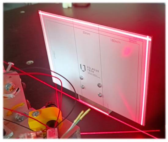
Figure 8.
Calibration plate for laser scanner.
From Figure 8, it can be seen that the calibration plate has linear markings indicating the robot’s dimensions and a tolerance of 10 mm. The camera is positioned straight, while the upper laser pointer, which will be used in the experiment, is tilted at an angle, lining up with the laser projection at the bottom of the calibration plate. According to Figure 2, angle ωg is equal to 40.5°. Other dimensions marked in red can also be estimated by using a 3D modeling program and a 3D model of the system. The following dimensions are determined in advance:
- ωg = 40.5°;
- d1 = 130 mm;
- θ1 = 6.5°;
- ωg = 40.5°;
- L1 = 24.43 mm;
- L2 = 180.12 mm;
- L3 = 18.58 mm.
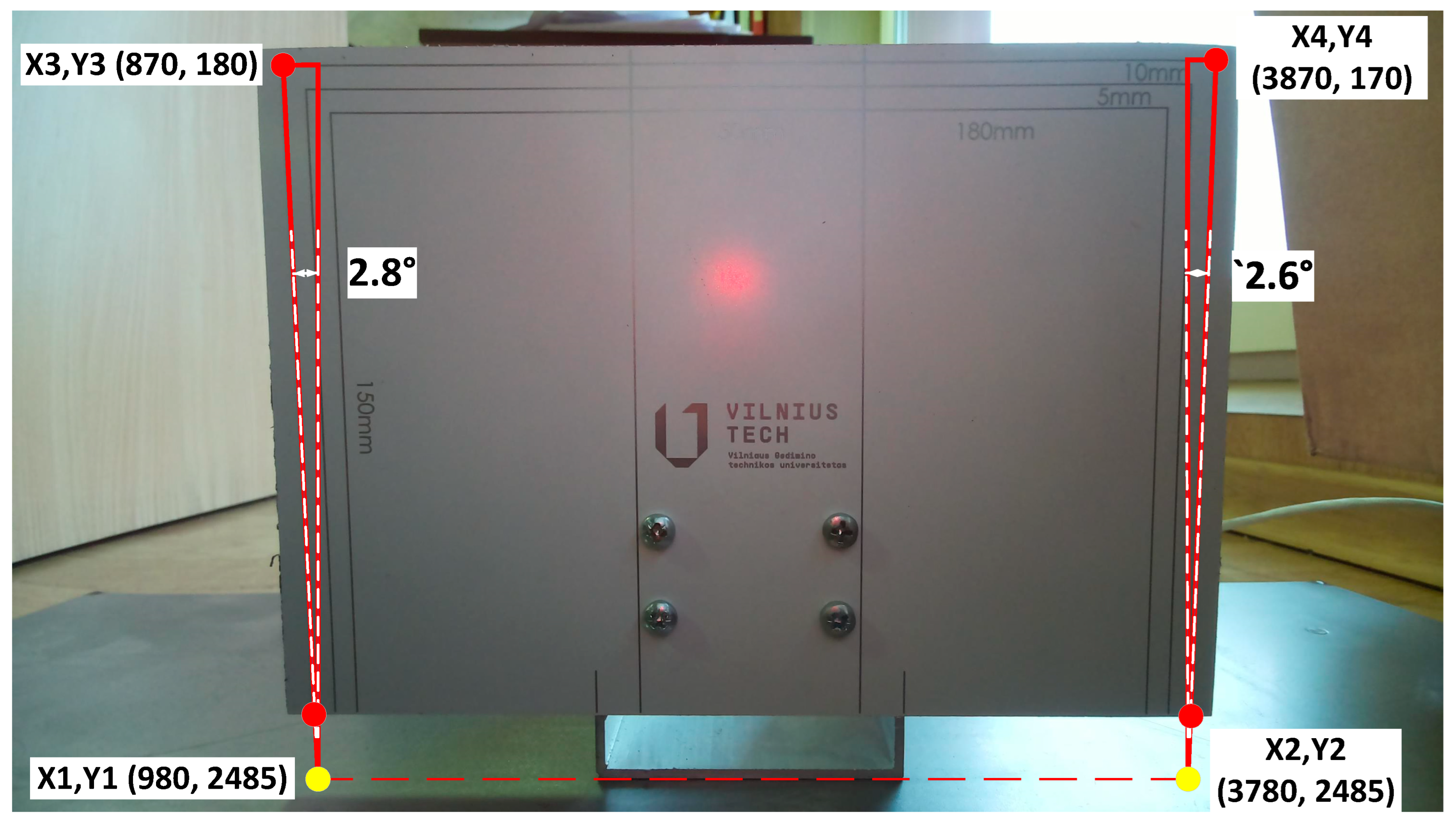
With these parameters, the distance from an object can be calculated, and then h1 is detected with the laser scanner. But to achieve this, the first camera has to be calibrated by estimating the image pixel relation to the real length of the captured projection. To achieve this, an image is taken with a laser scanner in the initial position by putting a calibration plate in the center 130 mm away from the scanner, as d1 is a measuring range. An image of the highest field of view and resolution is taken—4608 × 2592 pixels. The resulting image is shown in Figure 9.
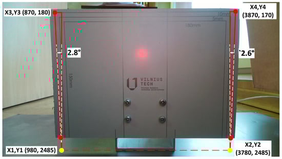
Figure 9.
Image of calibration plate taken with laser scanner system camera (red lines represent the scanning region and field-of-view distortion and white lines represent the angles of distortion).
The calibration plate is marked with lines representing the scanning region with specified values—width wr = 200 mm and height hr = 160 mm. To convert pixel size to the real length, firstly, the corners of the calibration plate are marked in the captured image as shown in Figure 8. Red corners represent the corners of the plate, and yellow corners are projections of the bottom corners of the scanning region, which are estimated geometrically via solidworks 2024 (Student’s version) modeling software. To find pixel real dimensions as width wpxi and height hpix, the following proportions are used, as defined in Equations (5) and (6):
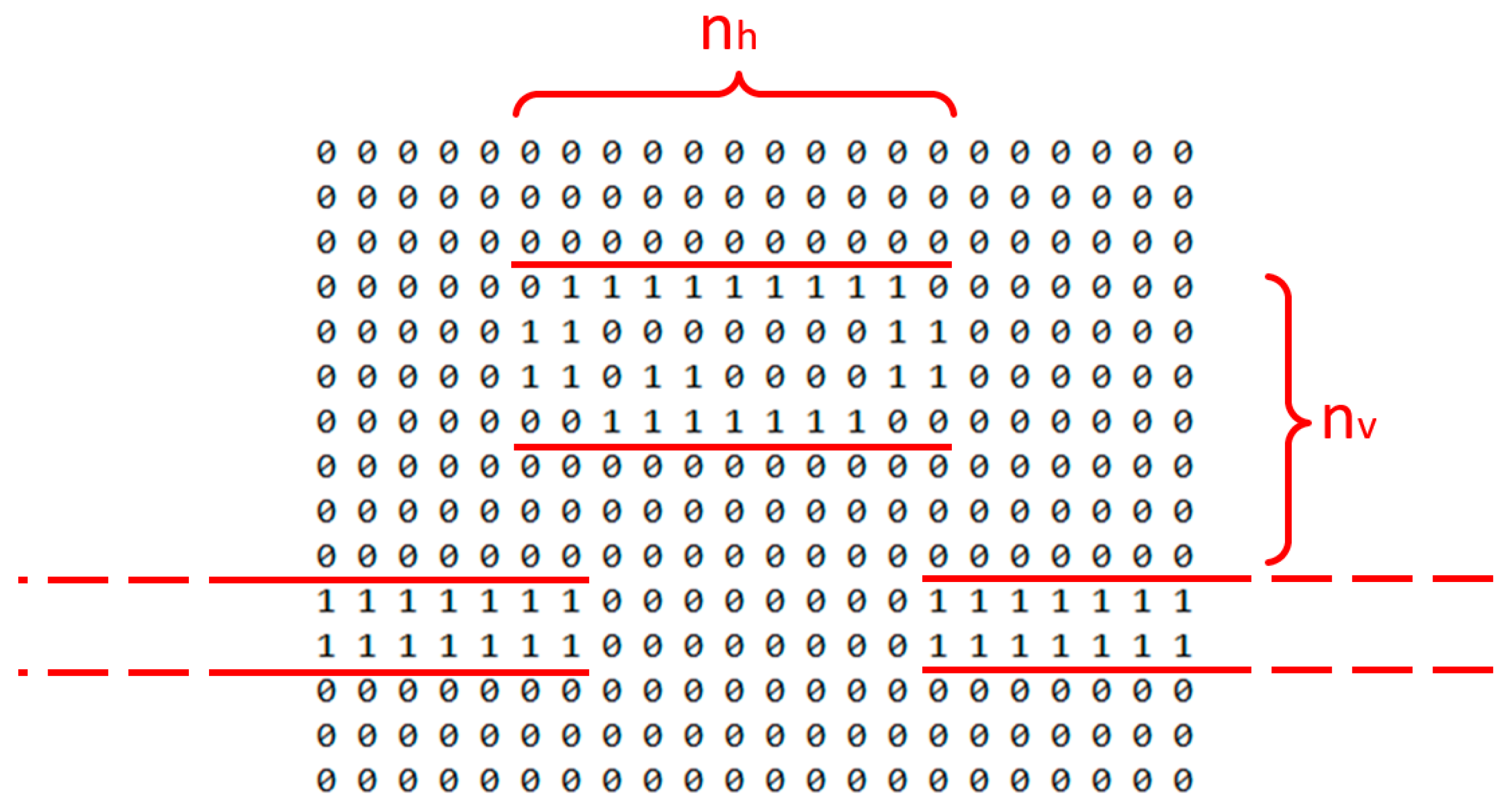
By calculating the image pixel width wpix and height hpix of the calibrated region, it is possible to directly measure the width and height of an obstacle based on the displacement and length of linear laser projections. In Figure 10, a simplified view of the pixel grid and the laser line projected on the obstacle is shown as an estimated data processing model.
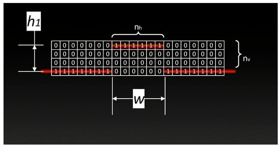
Figure 10.
Simplified laser scanner camera view with present obstacle and pixel grid (laser linear projection marked in red).
Pixels marked with 1 represent the detected color of the laser, while 0 s represent the filtered zone of a different color. The obstacle height can be calculated by the following formula:
where nv is the number of pixels shown vertically. Nevertheless, as seen in Figure 9, the vertical view is stretched, and the width at the bottom of the calibration plate and the top is different. This happens because the camera used has a very wide field of view, which results in a slightly distorted view on the sides. Because of this, width has to be compensated depending on the distance from the obstacle, which is determined by displacement h1. Another factor that significantly affects width calculation is the camera perspective angle from different distances, which is visually presented in Figure 11.
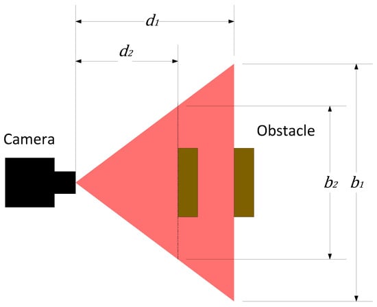
Figure 11.
Camera object perspective from different distances (red color represents laser linear projection and brown color represents obstacle positions).
If an obstacle is closer to the camera from the calibration plane, the width of the obstacle is perceived as bigger because d1 divided by d2 is proportional to b1 divided by b2. Because of this, the calculated width must be additionally multiplied by the ratio of d1/d2. Taking these aspects into account, the obstacle width can be calculated with the following formula:
where nh is the number of pixels shown horizontally and θk is the compensation angle, and the width wr is 180 mm, which can be seen in Figure 9. The compensation angle increases proportionally from the center to the left or right corner of the picture because of the wide-angle camera view distortion. The compensation angle is slightly different on each side because of system deviations. For this reason, the average value is taken—θk = 2.7°.
2.3. Image Processing
As mentioned before, the camera takes 4608 × 2592-pixel size images. To be able to recognize obstacles which are marked with linear laser projections, it is necessary to filter unnecessary colors from the raw camera picture. There are many models which are used for image processing. For this project, the hue, saturation, value (HSV) model is used, programmed with the C++ language, integrating OpenCV open-source libraries for faster computational processing. The HSV method is more advantageous than regular RGB color processing, most importantly because it is more robust in terms of external lighting changes. It is able to evaluate color intensity [30,31,32]. For example, an unusual color that is being searched for can have different intensities in the photo because of external light and shadows, and the HSV method allows the color to be distinguished. HSV color space is shown in Figure 12, defined by three parameters according to the model’s name, as stated previously.

Figure 12.
HSV color space graph and parameters [33].
Hue defines the different color regions and has a value from 0° to 360°. When using OpenCV libraries, hue values are scaled between 0 and 180. Value defines brightness, and saturation defines color depth. Both of these values range between 0 and 255.
For this experiment, two red color ranges were chosen for the upper and lower thresholds. Also, a saturation value of 10,000 and a gain value of 2 were chosen to allow the camera to take darker images and mimic a sewer-like view without outside lighting. For the lower range, values from [0, 50, 50] to [10, 255, 255] were selected, while for the upper range, values from [170, 50, 50] to [180, 255, 255] were selected. This range allows for the detection of shades of red of varying intensity. After that, the image is transformed into a grayscale, as shown in Figure 13.
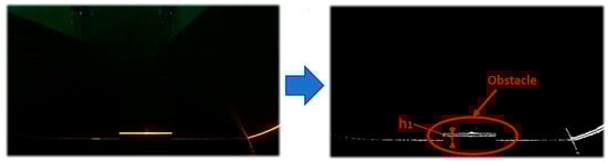
Figure 13.
Original image of the present obstacle taken with an RGB camera and transformed to grayscale.
Filtered pixels are changed to a white color with a value of 255, and background pixels are changed to black with a value of 0. This simplifies the calculations used to find regions of interest. Another factor that greatly affects image recognition accuracy and processing speed is segmentation. Reading the value of every pixel and saving it in the memory is computationally demanding. It is more convenient to separate the image into larger square segments, as shown in Figure 14.
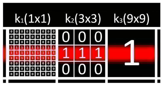
Figure 14.
Simplified view of the original image with different segmentation values (red color represents laser linear projection).
The described procedure allows for a reduction in memory load. Segmentation value will be defined as k (nh2, nv2), where nh2 represents how many pixels are stored horizontally in the analyzed squared region, and nv2 represents the number of pixels stored vertically. Looking at Figure 11, it can be seen that depending on the segmentation value, the detected laser line can be divided into several pixels. For this reason, the calculation of pixels horizontally and vertically is performed as shown in Figure 15.
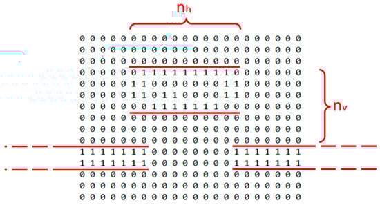
Figure 15.
Obstacle width and height of pixel selection from the processed image (red lines represent laser linear projection width).
The figure above shows the segmentation of a real camera image taken from the experiment. The number of pixels stored vertically is calculated from the top of the straight-line projection of the laser to the top of the highest projection disturbed by the obstacle. This logic is applied because the object observed during the experiment is of a square shape, so the top of the object can be assumed as a straight line in this case. For this experiment, segmentation values of 32 × 32, 16 × 16, 9 × 9, and 4 × 4 are used for each of the different measurements.
3. Results
According to the explained methodology, an experiment was performed and data were gathered. In total, 160 measurements of the distance from and the width of obstacles were taken, including four different obstacles that were 5, 10, 30, and 50 mm wide. The deviation between real and measured dimensions was calculated, and the following formulas are used for statistical analysis:
where xi is the measurement deviation, is the mean, n—number of measurements with corresponding obstacle and segmentation value, si—deviation from the mean value, and s—standard deviation. During each distance increment from 5 to 50 mm, an image was taken, and each step was increased by 5 mm, moving closer to an obstacle. All images were processed using four different segmentation values of 32 × 32, 16 × 16, 8 × 8, and 4 × 4. The collected data and analysis are presented further.
3.1. Distance Measurements
Measurements were carried out starting from the thinnest obstacle, which was 5 mm wide. The results of different segmentation values are compared in a column-type diagram for a clearer view. The diagram is presented in Figure 16.
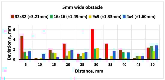
Figure 16.
Results of distance measurements with a 5 mm wide obstacle.
The horizontal axis represents distance increments, and the laser scanner is moving closer to an obstacle from an initial position, which is 130 mm away from the obstacle. The vertical axis represents deviation from the mean of the measured distance and the real distance estimated by the industrial robot movement, which ensures ±0.1 mm accuracy. At the top of the table, different segmentation values are shown. Each segmentation value has a corresponding standard deviation value. Looking at Figure 15, it is noticeable that the standard deviation is highest with 32 × 32 segmentation and gradually reduces as the segmentation value is lowered. Nevertheless, the lowest deviation is achieved with a 9 × 9 segmentation value. This would indicate that the 9 × 9 value is more optimal compared to the 4 × 4, as it generates smaller deviation and requires fewer computational resources for processing optical information.
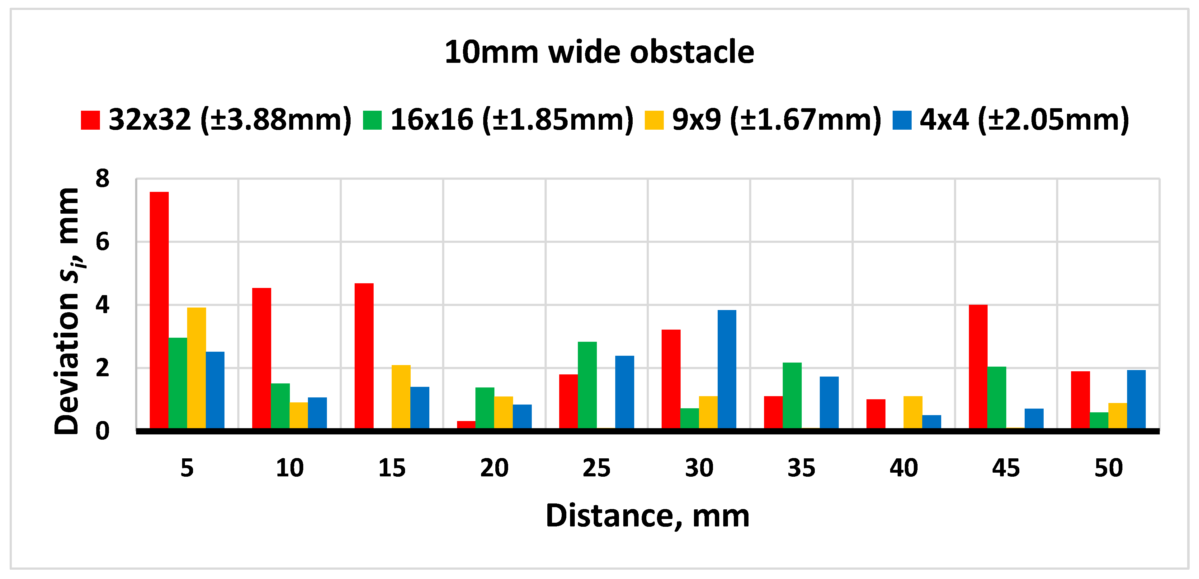
The experiment is further proceeded by measuring a 10 mm wide obstacle. The results are shown in Figure 17.
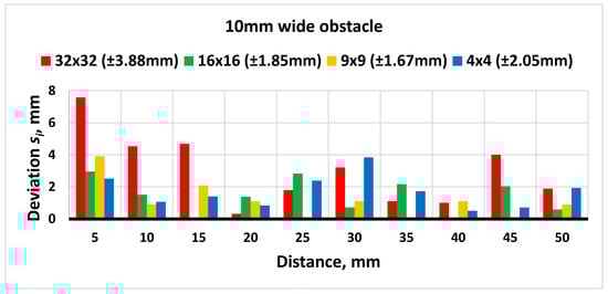
Figure 17.
Results of distance measurements with a 10 mm wide obstacle.
Looking at the figure above, it can be noticed that the standard deviation has a similar tendency when measuring a 10 mm wide obstacle. It is highest at a segmentation value of 32 × 32. Then, increasing the number of pixels processed, the lowest deviation is reached with a 9 × 9 value. Decreasing the value further increases the deviation.
The experiment is further proceeded by measuring a 30 mm wide obstacle. The obtained results are shown in Figure 18.
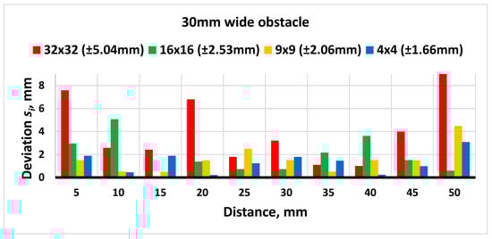
Figure 18.
Results of distance measurements with a 30 mm wide obstacle.
Looking at the figure above, it can be seen that, unlike the first two obstacles, lowering the segmentation value up to 4 × 4 gradually reduces deviation, although the most significant difference still remains between 32 × 32 and 16 × 16. Also, the largest error of ±5.04 was measured with a 32 × 32 segmentation value during this experiment.
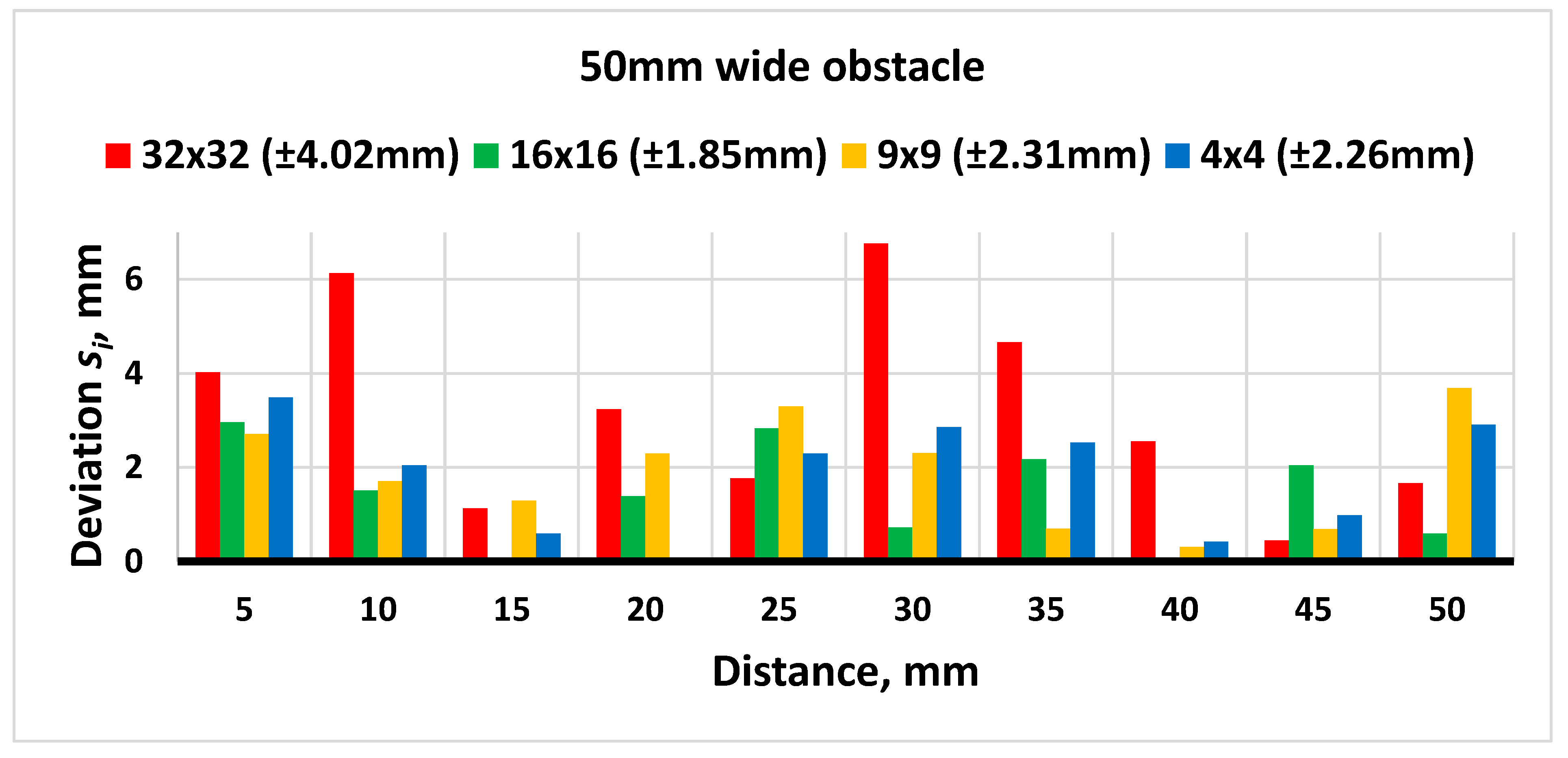
The experiment proceeded with the measurement of a 30 mm wide obstacle. The results are shown in Figure 19.
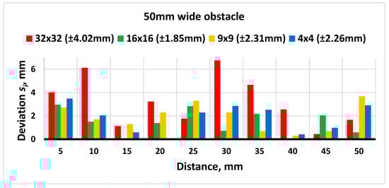
Figure 19.
Results of distance measurements with a 50 mm wide obstacle.
Looking into the results acquired from measuring a 50 mm wide obstacle, it is noticeable that the highest deviation remains when the segmentation value is 32 × 32. Nevertheless, the lowest resolution is reached with a segmentation value of 16 × 16, and this is increased by further lowering the segmentation to 9 × 9 and 4 × 4.
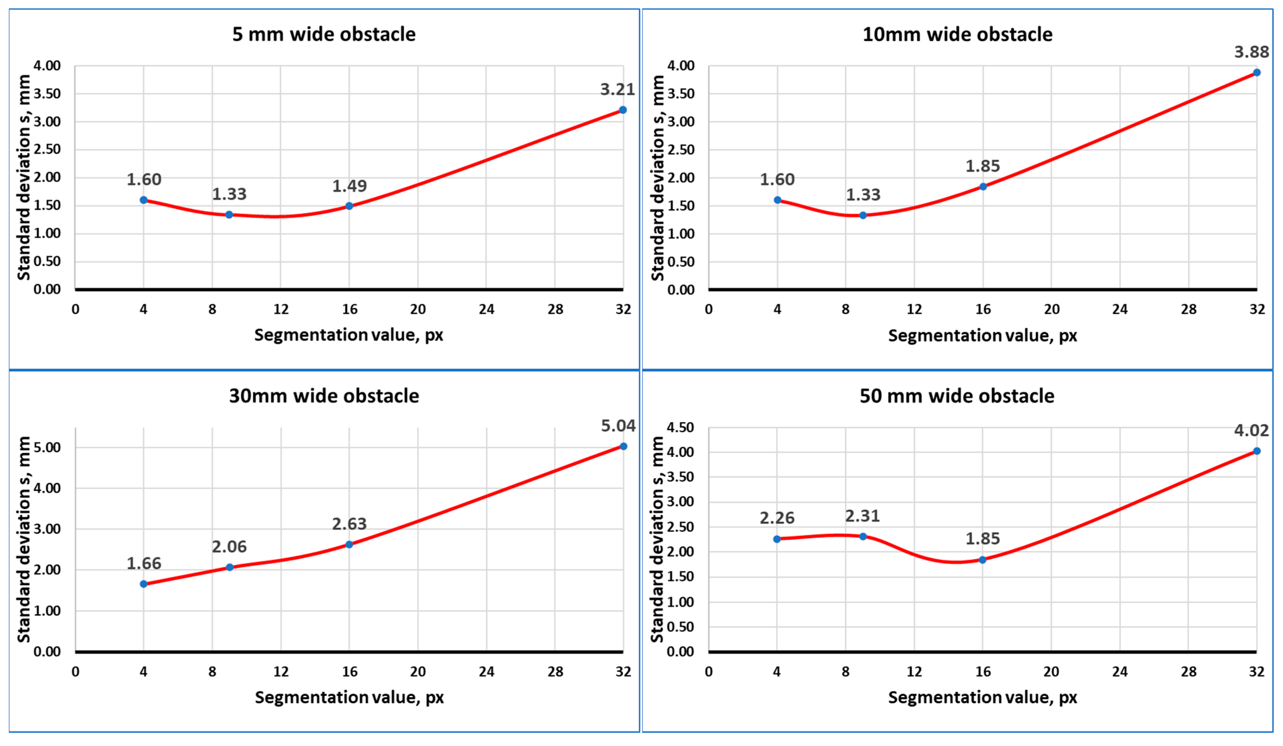
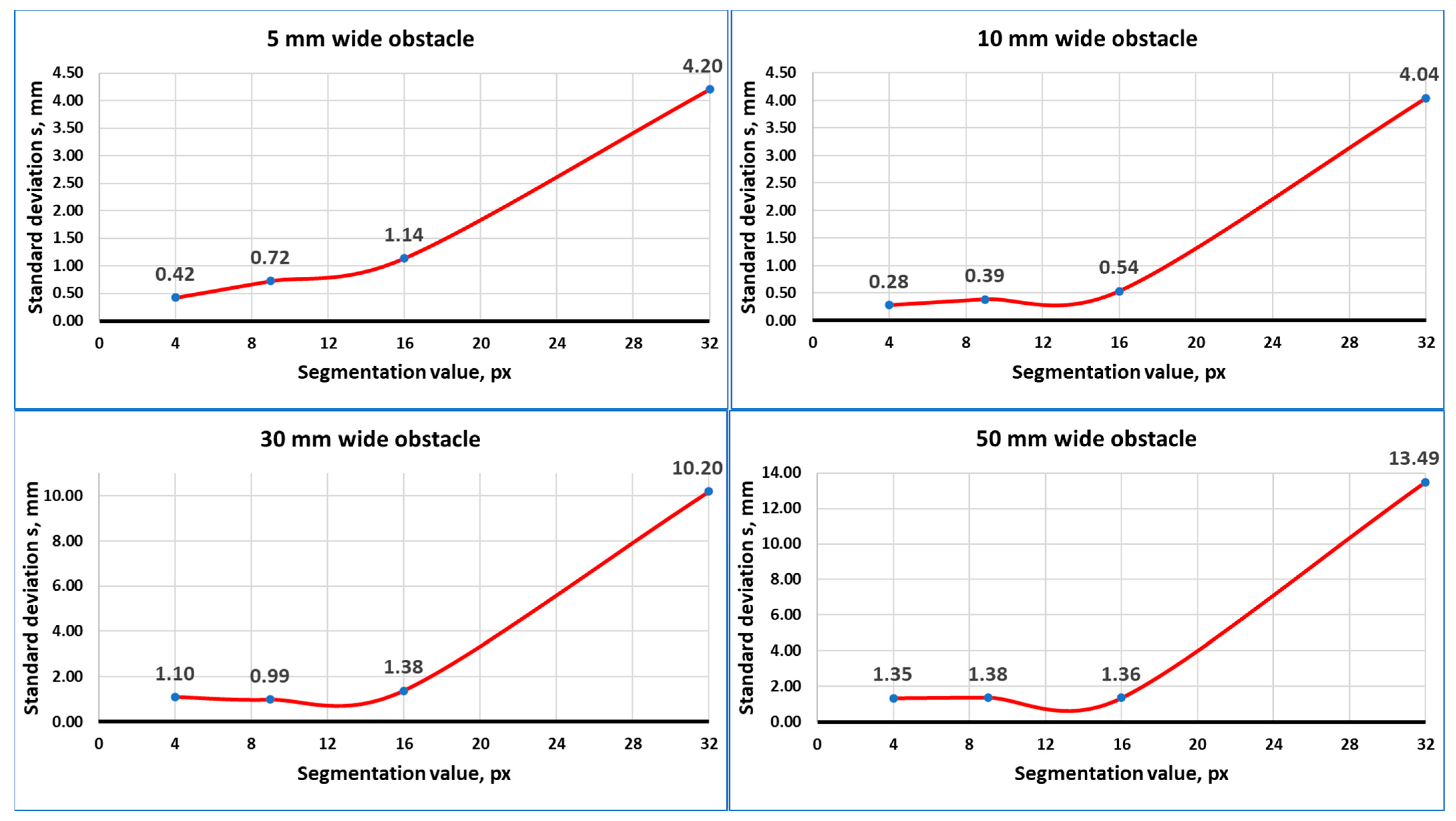
Based on an analysis of distance measurements acquired during an experiment, it was observed that changing the segmentation value greatly affects distance measurement accuracy. Nevertheless, the relation is not linear, as seen in Figure 20.
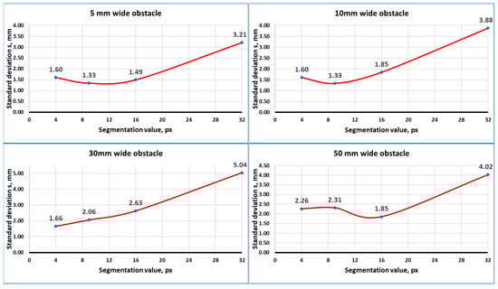
Figure 20.
Standard deviation values of distance measurements.
The lowest deviation was reached using a segmentation value of 9 × 9. However, it is noticeable that while measuring wider obstacles (30 and 50 mm), the lowest deviation varies between 4 × 4 and 16 × 16. This can be affected by the reflection of laser light, which is more noticeable on wider areas of surfaces. Reflection introduces noise in the image, which makes the laser beam projection appear thicker and more distorted, as shown in Figure 21.
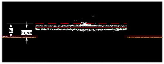
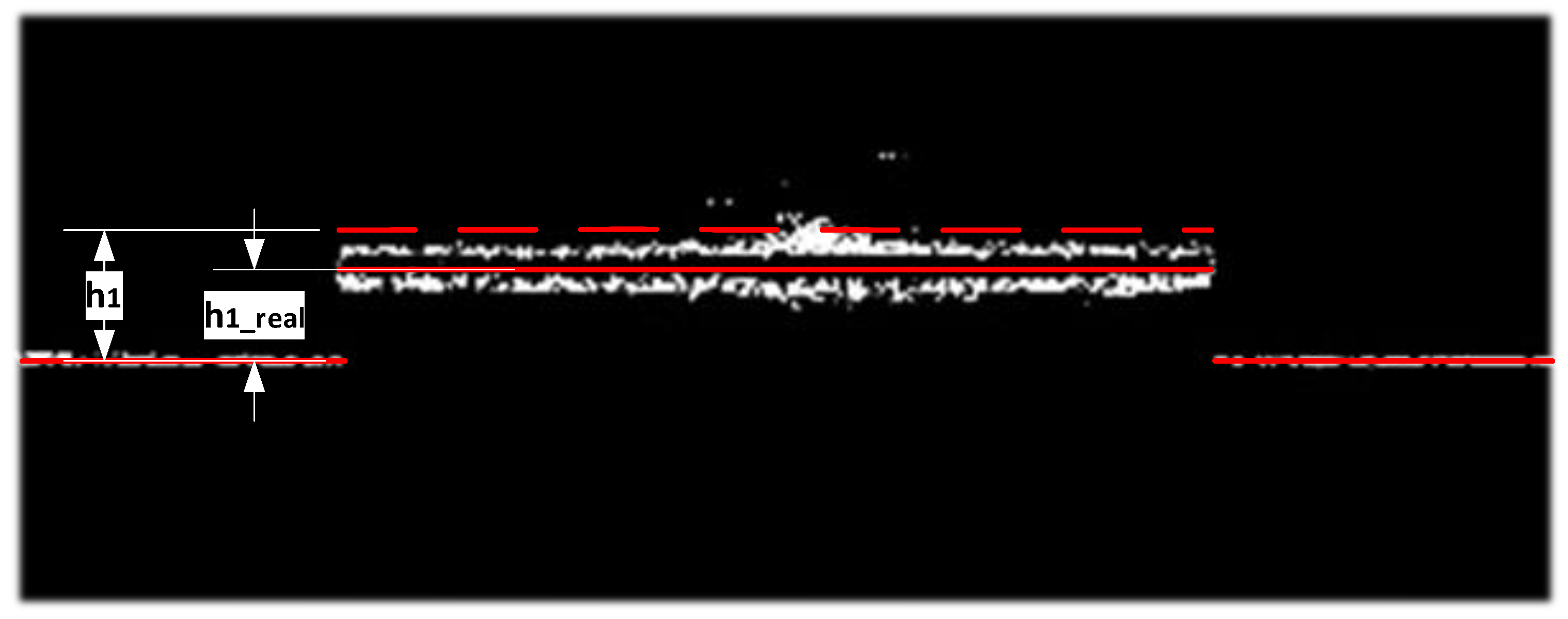
Figure 21.
Filtered image processing (red lines represent center position of laser linear projection and dashed line estimated upper position).
It is noticeable that the laser line projected on the obstacle is thicker than the line projected on the ground due to geometrical conditions. Because of this measured displacement, h1 is between the estimated lines by the algorithm, which is larger than the displacement between the line projected on the ground and the nominal real line corresponding to h_real shown in the figure above. Moreover, additional peaks of reflected light also increase h1 and influence measurement deviation. To compensate for the reflection influence coefficient—a is adjusted, which is expressed in Formula (2):
Using known values from the calibrated system, the geometric value of coefficient a is equal to 5.6. Nevertheless, experimentally, the lowest deviations were achieved with the value of 3.2. A smaller value of a compensates for the higher displacement estimated by the calculation algorithm.
It is also possible to reduce picture noise with saturation and gain values of the camera, which reduces the received light, resulting in a darker picture with fewer reflections. Nevertheless, these values have already sufficiently decreased according to the experimental environment; therefore, further reducing these values makes laser projection discontinuous, leading to calculation errors.
3.2. Width Measurements
The image processing algorithm also calculates the width, which is necessary for determining the occupancy grid of the scanned environment. Width is calculated using formula 8, where h2 is the measured laser projection deviation and d2 is the calculated distance from an obstacle. The camera’s field of view develops slight distortion in the corners, as previously explained in Figure 9. For this reason, h2 has a slight influence on width calculation accuracy. The results of the experimental width measurements for each obstacle are shown in Figure 22.
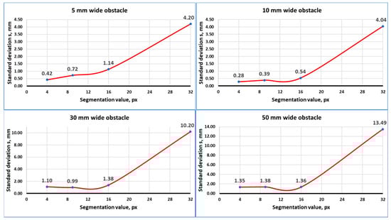
Figure 22.
Standard deviation values of obstacle width measurements.
From the figure above, it is noticeable that the standard deviation pattern of width measurements is similar to that of distance measurements. Nevertheless, with a segmentation value of 32 × 32, deviations are significantly higher, especially with wider obstacles of 30 and 50 mm. Additional noise at the corners of processed obstacle laser projection taken in the image influences the measured width more significantly, the larger the segmentation value. Also, the perspective of the camera from different distances increases the error when the obstacle width is higher, which can be seen from gathered data, as the wider the obstacle, the more significant the increase in deviations.
Similarly, as with distance measurement, it is not worth going lower than a 9 × 9 segmentation value, as deviations do not fall or decrease by a very small margin, and such distances are not significant for navigation purposes. Moreover, computational resources can be saved considerably by choosing 9 × 9 or even 16 × 16 segmentation values.
3.3. Integration into the Mobile Robot
After calibrating and testing the laser marker and the RGB camera-based measurement system, it can be applied to the intended autonomous sewer robot. Calibration of the measurement system with the industrial robot was performed according to the designed mobile robot prototype geometry. Laser makers and cameras could then be assembled directly on the mobile robot platform shown in Figure 23.
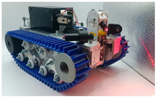
Figure 23.
Autonomous sewer robot prototype.
There are marked lines for adjusting the angles of each laser, or the same calibration plate as used in the experiment can be used to calibrate the system. The prototype also includes previously mentioned sensors, including LiDAR and a gyroscope/accelerometer module. The prototype is made of lightweight aluminum and has rubber belts for better friction. Also, all parts are either made from aluminum, 3D-printed, or zinc-coated to prevent corrosion. The tank-type chassis allows the robot to pass through obstacles that are 4 cm high, but for more accurate navigation, only obstacles up to 2 cm are considered acceptable. This platform is suitable for further experiments in harsher sewer-like environments.
4. Discussion and Conclusions
A laser scanner consisting of four linear laser markers and an RGB camera provides a versatile obstacle detection and measurement system. Four laser pointers allow for the detection of obstacles present in a rectangular field of view, which can easily cover the mobile robot’s dimensions.
For image processing, we decided to filter red laser light color from the background using low camera saturation and gain values. This created a darker image, reducing light reflections. For distance and width measurement, filtered image data were transformed into a one-dimensional array storing relevant data for both dimensions. An array could then be used for direct fusion with LiDAR data, expanding the field of the mobile sewer robot system.
During experiments, the accuracy of distance measurement was determined using one laser marker, as a similar procedure was performed with all four laser markers. The lowest distance measurement deviation was ±1.33 mm, and this was reached using a 9 × 9 segmentation value with 4608 × 2592 pixel resolution. This deviation was reached measuring a 10 mm wide obstacle with a range of 130 mm. It was observed that the deviation was increased by increasing the obstacle width, which was influenced by the surface reflection of aluminum material, which was more reflective compared to the ground. Nevertheless, 1.33 mm is sufficient for navigation purposes. Moreover, reducing the segmentation value to lower than 9 × 9 increased accuracy very minimally, or in some cases, higher deviation was encountered. Also, lowering the segmentation value increased computational resources.
During the experiment, the obstacle width was also tested, reaching the lowest deviation of ±0.28 mm, then measuring a 10 mm wide obstacle with a 4 × 4 segmentation value. However, the 9 × 9 segmentation value was more efficient, as the increase in deviation was minimal. Similarly, as with distance measurement, an increase in obstacle width increases deviation, which is influenced by surface reflection and also by camera perspective.
The tested optical obstacle detection and distance measurement system allows for accurate detection of obstacles in a short range of 130 mm. Further experiments are needed to combine all four laser markers to detect obstacles attached to the walls and the ceiling. Also, further experimentation is needed to fuse laser scanner data with LiDAR data.
Moreover, mobile robot rotation and swinging from uneven ground surface can also influence laser scanner measurements, as the ground or wall can also deform the laser projection. For this reason, an accelerometer and a gyroscope signal should be added for relative and absolute measurement of mobile robot rotation in each axis for laser beam projection compensation.
Author Contributions
Conceptualization, V.U. and V.B.; methodology, V.B.; software, J.N.; validation, V.U., A.D. and J.N.; formal analysis, A.D.; investigation, V.U.; resources, V.B.; data curation, J.N.; writing—original draft preparation, V.U.; writing—review and editing, V.B. and A.D.; visualization, V.U.; supervision, V.B.; project administration, A.D.; funding acquisition, V.B. All authors have read and agreed to the published version of the manuscript.
Funding
The research was supported by Joint Research Collaborative Seed Grant Program between Taiwan Tech and Vilnius Gediminas Technical University (Grant No Taiwan Tech—VILNIUS TECH-2024-03).
Data Availability Statement
The original contributions presented in this study are included in the article. Further inquiries can be directed to the corresponding author(s).
Conflicts of Interest
The authors declare no conflicts of interest.
References
- Akhshirsh, G.S.; Al-Salihi, N.K.; Hamid, O.H. A Cost-Effective GPS-Aided Autonomous Guided Vehicle for Global Path Planning. Bull. Electr. Eng. Inform. 2021, 10, 650–657. [Google Scholar] [CrossRef]
- Qin, H.; Shao, S.; Wang, T.; Yu, X.; Jiang, Y.; Cao, Z. Review of Autonomous Path Planning Algorithms for Mobile Robots. Drones 2023, 7, 211. [Google Scholar] [CrossRef]
- Belkin, I.; Abramenko, A.; Yudin, D. Real-Time Lidar-Based Localization of Mobile Ground Robot. Procedia Comput. Sci. 2021, 186, 440–448. [Google Scholar] [CrossRef]
- Ou, X.; You, Z.; He, X. Local Path Planner for Mobile Robot Considering Future Positions of Obstacles. Processes 2024, 12, 984. [Google Scholar] [CrossRef]
- Li, K.; Gong, X.; Tahir, M.; Wang, T.; Kumar, R. Towards Path Planning Algorithm Combining with A-Star Algorithm and Dynamic Window Approach Algorithm. Int. J. Adv. Comput. Sci. Appl. 2023, 14, 511–519. [Google Scholar] [CrossRef]
- Alshammrei, S.; Boubaker, S.; Kolsi, L. Improved Dijkstra Algorithm for Mobile Robot Path Planning and Obstacle Avoidance. Comput. Mater. Contin. 2022, 72, 5939–5954. [Google Scholar] [CrossRef]
- Tatsch, C.; Bredu, J.A.; Covell, D.; Tulu, I.B.; Gu, Y. Rhino: An Autonomous Robot for Mapping Underground Mine Environments. In Proceedings of the 2023 IEEE/ASME International Conference on Advanced Intelligent Mechatronics (AIM), Seattle, WA, USA, 28–30 June 2023; pp. 1166–1173. [Google Scholar] [CrossRef]
- Assaf, E.H.; von Einem, C.; Cadena, C.; Siegwart, R.; Tschopp, F. High-Precision Low-Cost Gimballing Platform for Long-Range Railway Obstacle Detection. Sensors 2022, 22, 474. [Google Scholar] [CrossRef]
- Shamshiri, R.R.; Navas, E.; Dworak, V.; Auat Cheein, F.A.; Weltzien, C. A Modular Sensing System with CANBUS Communication for Assisted Navigation of an Agricultural Mobile Robot. Comput. Electron. Agric. 2024, 223, 109112. [Google Scholar] [CrossRef]
- You, H.; Xu, F.; Ye, Y.; Xia, P.; Du, J. Adaptive LiDAR Scanning Based on RGB Information. Autom. Constr. 2024, 160, 105337. [Google Scholar] [CrossRef]
- Weinmann, K.; Simske, S. Design of Bluetooth 5.1 Angle of Arrival Homing Controller for Autonomous Mobile Robot. Robotics 2023, 12, 115. [Google Scholar] [CrossRef]
- Wang, H.; Yin, Y.; Jing, Q. Comparative Analysis of 3D LiDAR Scan-Matching Methods for State Estimation of Autonomous Surface Vessel. J. Mar. Sci. Eng. 2023, 11, 840. [Google Scholar] [CrossRef]
- Yao, S.; Guan, R.; Huang, X.; Li, Z.; Sha, X.; Yue, Y.; Lim, E.G.; Seo, H.; Man, K.L.; Zhu, X.; et al. Radar-Camera Fusion for Object Detection and Semantic Segmentation in Autonomous Driving: A Comprehensive Review. IEEE Trans. Intell. Veh. 2024, 9, 2094–2128. [Google Scholar] [CrossRef]
- Toderean, B.; Rusu-Both, R.; Stan, O. Guidance and Safety Systems for Mobile Robots. In Proceedings of the 2020 IEEE International Conference on Automation, Quality and Testing, Robotics (AQTR), Cluj-Napoca, Romania, 21–23 May 2020. [Google Scholar] [CrossRef]
- Wang, T.; Guan, X. Research on Obstacle Avoidance of Mobile Robot Based on Multi-Sensor Fusion; Springer International Publishing: Berlin/Heidelberg, Germany, 2020; Volume 928, ISBN 9783030152345. [Google Scholar]
- Sarmento, J.; Neves dos Santos, F.; Silva Aguiar, A.; Filipe, V.; Valente, A. Fusion of Time-of-Flight Based Sensors with Monocular Cameras for a Robotic Person Follower. J. Intell. Robot. Syst. Theory Appl. 2024, 110, 30. [Google Scholar] [CrossRef]
- Lin, Z.; Gao, Z.; Chen, B.M.; Chen, J.; Li, C. Accurate LiDAR-Camera Fused Odometry and RGB-Colored Mapping. IEEE Robot. Autom. Lett. 2024, 9, 2495–2502. [Google Scholar] [CrossRef]
- Gatesichapakorn, S.; Takamatsu, J.; Ruchanurucks, M. ROS Based Autonomous Mobile Robot Navigation Using 2D LiDAR and RGB-D Camera. In Proceedings of the 2019 First International Symposium on Instrumentation, Control, Artificial Intelligence, and Robotics (ICA-SYMP), Bangkok, Thailand, 16–18 January 2019; pp. 151–154. [Google Scholar] [CrossRef]
- Liu, Y.; Zhang, W.; Li, F.; Zuo, Z.; Huang, Q. Real-Time Lidar Odometry and Mapping with Loop Closure. Sensors 2022, 22, 4373. [Google Scholar] [CrossRef] [PubMed]
- Miranda, J.C.; Arnó, J.; Gené-Mola, J.; Lordan, J.; Asín, L.; Gregorio, E. Assessing Automatic Data Processing Algorithms for RGB-D Cameras to Predict Fruit Size and Weight in Apples. Comput. Electron. Agric. 2023, 214, 108302. [Google Scholar] [CrossRef]
- De Silva, V.; Roche, J.; Kondoz, A. Robust Fusion of LiDAR and Wide-Angle Camera Data for Autonomous Mobile Robots. Sensors 2018, 18, 2730. [Google Scholar] [CrossRef]
- Naga, P.S.B.; Hari, P.J.; Sinduja, R.; Prathap, S.; Ganesan, M. Realization of SLAM and Object Detection Using Ultrasonic Sensor and RGB-HD Camera. In Proceedings of the 2022 International Conference on Wireless Communications Signal Processing and Networking (WiSPNET), Chennai, India, 24–26 March 2022; pp. 167–171. [Google Scholar] [CrossRef]
- Yang, L.; Li, P.; Qian, S.; Quan, H.; Miao, J.; Liu, M.; Hu, Y.; Memetimin, E. Path Planning Technique for Mobile Robots: A Review. Machines 2023, 11, 980. [Google Scholar] [CrossRef]
- Fu, G.; Corradi, P.; Menciassi, A.; Dario, P. An Integrated Triangulation Laser Scanner for Obstacle Detection of Miniature Mobile Robots in Indoor Environment. IEEE/ASME Trans. Mechatron. 2011, 16, 778–783. [Google Scholar] [CrossRef]
- Ding, D.; Ding, W.; Huang, R.; Fu, Y.; Xu, F. Research Progress of Laser Triangulation On-Machine Measurement Technology for Complex Surface: A Review. Meas. J. Int. Meas. Confed. 2023, 216, 113001. [Google Scholar] [CrossRef]
- So, E.W.Y.; Munaro, M.; Michieletto, S.; Antonello, M.; Menegatti, E. Real-Time 3D Model Reconstruction with a Dual-Laser Triangulation System for Assembly Line Completeness Inspection. In Advances in Intelligent Systems and Computing; Springer: Berlin/Heidelberg, Germany, 2013; Volume 194, pp. 707–716. [Google Scholar] [CrossRef]
- Ai, C.; Qi, Z.; Zheng, L.; Geng, D.; Feng, Z.; Sun, X. Research on Mapping Method Based on Data Fusion of Lidar and Depth Camera. In Proceedings of the 2021 4th International Conference on Advanced Electronic Materials, Computers and Software Engineering (AEMCSE), Changsha, China, 26–28 March 2021; pp. 360–365. [Google Scholar] [CrossRef]
- Kolar, P.; Benavidez, P.; Jamshidi, M. Survey of Datafusion Techniques for Laser and Vision Based Sensor Integration for Autonomous Navigation. Sensors 2020, 20, 2180. [Google Scholar] [CrossRef]
- Hassani, S.; Dackermann, U.; Mousavi, M.; Li, J. A Systematic Review of Data Fusion Techniques for Optimized Structural Health Monitoring. Inf. Fusion 2024, 103, 102136. [Google Scholar] [CrossRef]
- Yang, K.; Wang, K.; Bergasa, L.M.; Romera, E.; Hu, W.; Sun, D.; Sun, J.; Cheng, R.; Chen, T.; López, E. Unifying Terrain Awareness for the Visually Impaired through Real-Time Semantic Segmentation. Sensors 2018, 18, 1506. [Google Scholar] [CrossRef] [PubMed]
- Le, N.M.D.; Nguyen, N.H.; Nguyen, D.A.; Ngo, T.D.; Ho, V.A. ViART: Vision-Based Soft Tactile Sensing for Autonomous Robotic Vehicles. IEEE/ASME Trans. Mechatron. 2023, 29, 1420–1430. [Google Scholar] [CrossRef]
- Maitlo, N.; Noonari, N.; Arshid, K.; Ahmed, N.; Duraisamy, S. AINS: Affordable Indoor Navigation Solution via Line Color Identification Using Mono-Camera for Autonomous Vehicles. In Proceedings of the 2024 IEEE 9th International Conference for Convergence in Technology (I2CT), Pune, India, 5–7 April 2024. [Google Scholar] [CrossRef]
- Chen, W.-L.; Kan, C.-D.; Lin, C.-H.; Chen, Y.-S.; Mai, Y.-C. Hypervolemia Screening in Predialysis Healthcare for Hemodialysis Patients Using Fuzzy Color Reason Analysis. Int. J. Distrib. Sens. Netw. 2017, 13, 155014771668509. [Google Scholar] [CrossRef]


Disclaimer/Publisher’s Note: The statements, opinions and data contained in all publications are solely those of the individual author(s) and contributor(s) and not of MDPI and/or the editor(s). MDPI and/or the editor(s) disclaim responsibility for any injury to people or property resulting from any ideas, methods, instructions or products referred to in the content. |
© 2025 by the authors. Licensee MDPI, Basel, Switzerland. This article is an open access article distributed under the terms and conditions of the Creative Commons Attribution (CC BY) license (https://creativecommons.org/licenses/by/4.0/).