Transition Process Control of Tiltrotor Aircraft Based on Fractional-Order Model Reference Adaptive Control

Abstract

To address the critical challenge of controlling tiltrotor aircraft during transition mode, this paper proposes a fractional-order model reference adaptive control (FO-MRAC) method based on the unique modeling of the tiltrotor aircraft. A nonlinear model capturing the dynamic characteristics of the tiltrotor aircraft during the transition mode is developed based on an accurate analysis of the forces and moments acting on key components. This model is subsequently linearized to obtain a stable flight envelope. Considering the complexity of transition, the FO-MRAC method is designed based on the shift of the equilibrium point for superior parameter tuning and disturbance rejection. Then, the stability of the closed-loop system is analyzed using the Lyapunov stability theory. Finally, an experimental platform is constructed to verify the validity of the aerodynamic modeling and the designed control method.

1. Introduction

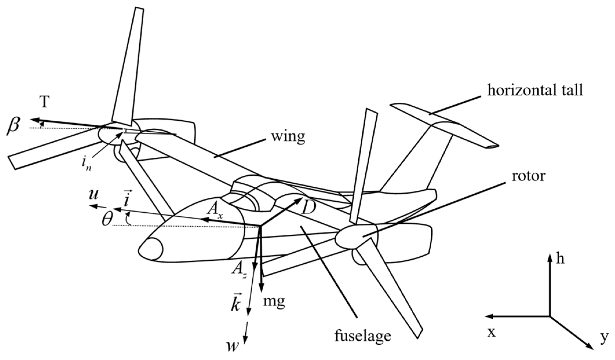
As a unique type of aerial vehicle that combines the operational characteristics of both fixed-wing airplanes and helicopters, the tiltrotor aircraft has been a hot research point in recent years. On one hand, traditional helicopters are constrained by the compressibility of the advancing rotor blade and the flow separation on the retreating rotor blade, which typically restrict their maximum cruising speed. On the other hand, runways are necessary for the wheeled takeoff and landing of fixed-wing aircraft, imposing stringent infrastructure demands and limiting operational flexibility in certain environments. The tiltrotor aircraft, however, integrates the vertical takeoff, landing capabilities, and hovering proficiency inherent to helicopters with the high-speed cruising efficiency characteristic of turboprop airplanes. This advantage endows tiltrotor aircraft with extended endurance, lower costs, and enhanced maneuverability compared to conventional helicopters, which makes it highly promising for addressing future urban air transportation needs [1,2,3].

Tiltrotor aircraft operate in three distinct flight modes: airplane mode, tilt-transition mode, and helicopter mode [4]. Each wing is equipped with a rotor nacelle system rotating between 0 and 90 degrees, so that the seamless transitions between helicopter and airplane modes can be achieved [2]. During the tilt-transition stage, the nacelles gradually rotate towards the direction of flight, shifting the rotor thrust vector from providing vertical lift to generating forward thrust, thereby broadening the aircraft flight envelope [5]. Despite the benefits, some challenges, such as the high-order dynamics of the control model, strong nonlinearities, and severe control coupling, render traditional flight control methods insufficient for achieving stable control across the full flight envelope for tiltrotor aircraft [6,7], which promotes the research in this paper.

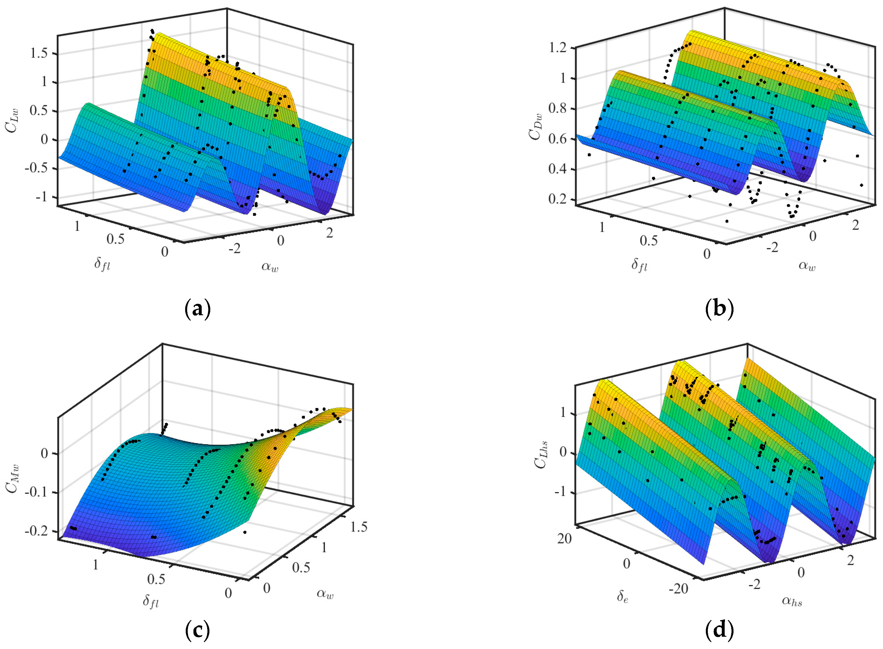
An accurate mathematical model of flight dynamics is crucial for the design of effective flight controllers. Therefore, extensive research has been conducted on the modeling of tiltrotor aircraft. Su et al. considered the dynamic characteristics of multiple tilting rotors and their gyroscopic and inertial coupling effects, established a comprehensive nonlinear rigid body dynamic model, and linearized it into a linear parameter variation (LPV) model [8]. Tischler et al. analyzed flight test data in the frequency domain to derive the transfer function of the tiltrotor model, which no longer required restrictive assumptions on model order or structure [9,10]. Liang et al. adopted a sub-component modeling method by separating the tiltrotor UAV into tilting and non-tilting parts and established their aerodynamic models, respectively [11]. Juhasz et al. further refined rotorcraft modeling by decoupling rigid-body and structural states, which were validated by using XV-15 and large civil tiltrotor platforms [12]. Distinct from the prior efforts that primarily focused on flight dynamics modeling and handling quality assessment, Lu et al. proposed a linear combination mode synthesis modeling approach that reflected stability derivatives throughout three operational modes to unify tiltrotor behaviors [13]. Despite these advancements, the complex interactions among key components, such as the fuselage, wings, tail, rotors, as well as their effects on overall flight dynamics, remain insufficiently detailed, indicating an urgent need for further research in this area.

With the continuous exploration of modern control theory and the refinement of tiltrotor aircraft mathematical models, more reliable controllers, such as incremental nonlinear dynamic inversion control [14], constrained optimal control [15], comprehensive robust control [16], active disturbance rejection control [17], model predictive control [18], and sliding mode control [19], have been developed to address the challenges of tiltrotor flight control. In addition, some emerging and widely adopted strategies, such as state-filtered disturbance rejection control [20] and multilayer neurocontrol of high-order uncertain nonlinear systems with active disturbance rejection [21], have also shown promising results in handling complex control problems. While these approaches have achieved flight control in a certain flight mode, they still lack sufficient adaptability and robustness for fine-tuning in the presence of transient effects and cross-mode nonlinear coupling, which arise from the nonlinear dynamic characteristics, time-varying parameter characteristics, and aerodynamic coupling effects during the tilt-transition mode. It should be noted that model reference adaptive control (MRAC) has emerged as an effective method for addressing nonlinear challenges due to its strong adaptability and robustness. In recent years, a number of MRAC-based schemes tailored for tiltrotor aircraft have been proposed. For instance, Liu et al. designed the radial-basis function (RBF) neural network and offline adaptation method to address the nonlinear problems in the control of a quad-tiltrotor UAV [22]. Wen et al. developed a hybrid adaptive control to address the actuator faults that occur during flight [23]. Shen et al. proposed a finite-time convergent sliding mode control based on an adaptive neural network extended state observer, which significantly improved disturbance rejection in tiltrotor UAVs [24]. These advancements highlight the ongoing efforts to enhance adaptability and robustness in tiltrotor flight control.

However, as the flight control requirement becomes increasingly complex, traditional integer-order control methods have shown their limitations due to the lack of flexible and refined parameter tuning capabilities. In contrast, FOC provides additional degrees of freedom for the controller by introducing fractional-order operators and taking advantage of their nonlocality and long memory characteristics. This characteristic enables FOC to achieve refined compensation for nonlinear transient processes by dynamically adjusting the historical state weights, thereby significantly improving the tracking accuracy and robustness during cross-mode dynamic transitions. In recent years, fractional-order control has emerged as a noteworthy approach. Lu et al. proposed a fractional-order sliding mode control strategy augmented with a disturbance observer, which exploited the memory-dependent properties of fractional calculus to achieve stable speed regulation of electromechanical systems [25]. Similarly, Zhang et al. constructed an electrospring model and introduced a fuzzy adaptive fractional-order controller, effectively improving the accuracy of the model and the robustness and adaptive ability of the control system [26]. Investigating the work above, fractional-order control is potentially suitable for tiltrotor aircraft flight control throughout all flight modes. Considering the rare application of FO-MRAC to tiltrotor aircraft, this paper conducts this research.

In this paper, by investigating the character of the unique aerodynamic modeling of the tiltrotor aircraft, a FO-MRAC is proposed for full-mode flight. Based on data from NASA research [27], a rigid-body model in the vertical plane is developed that is validated under open-loop configurations to ensure accuracy. Subsequently, the developed nonlinear model is used to calculate stable flight conditions so that the flight envelope can be determined. Then, model linearization is performed at certain stable points for controller design. To enhance parameter tuning ability during the full-mode flight, an FO-MRAC method applied with a fractional-order component is proposed for the flight control of the tiltrotor aircraft. Additionally, the simulations are conducted to verify the effectiveness of the fractional-order adaptive controller during the tilt-transition process within the stable flight envelope, which is also validated comprehensively by a hardware-in-the-loop platform.

The rest of this paper is organized as follows. In Section 2, the motion characteristic is investigated to establish the controlled model. In Section 3, trim analysis and stability characterization are discussed based on the constructed model. In Section 4, the design of the attitude control system based on FO-MRAC is presented. In Section 5, the simulations and experiments are conducted to demonstrate the effectiveness of the proposed control method. Finally, this paper is summarized in Section 6.

2. The Motion Modeling of Tiltrotor Aircraft

In this section, the aerodynamic characteristic of tiltrotor aircraft is investigated through a component-resolved approach to analyze the forces and moments generated by key aerodynamic components.

2.1. Component-Resolved Aerodynamic Modeling

To obtain the inherent characteristics of tiltrotor aircraft, it is necessary to investigate the component-resolved aerodynamics. As illustrated in Figure 1, the model adopts a modularized architecture comprising four principal subsystems: rotors, wings, fuselage, and horizontal tail.

Figure 1. Tiltrotor aircraft components and coordinate system.

Figure 1. Tiltrotor aircraft components and coordinate system.

• where $\overrightarrow{i}$ points in the direction of forward, and $\overrightarrow{k}$ points down, which satisfy the right-hand coordinate system. The state-space representation of the tiltrotor aircraft is derived as follows:

$$\dot{x}=f(x,u)$$

(1)

where $x={\left[w,u,\theta ,q,\Omega ,h,X\right]}^{\mathrm{T}}$ is the state vector, control input $u={\left[T,i_n\right]}^{\mathrm{T}}$ is the control input, where $w$ represents the vertical velocity component in body reference frame, $u$ represents horizontal velocity component in body reference frame, $\theta$ represents pitch angle, $q$ represents pitch rate, $\Omega$ represents rotor speed, $h$ represents tiltrotor altitude, $X$ represents horizontal location of aircraft, $T$ represents thrust from one rotor, $i_n$ represents nacelle angle, and $f(x,u)$ is the nonlinear function. Specifically, the function $f(x,u)$ is defined as

$$f(x,u)={\left[f_1(\theta ,q,u),f_2(\theta ,q,u),f_3(\theta ,q,u),f_4(\theta ,q,u),f_5(\theta ,q,u),f_6(\theta ,q,u),f_7(\theta ,q,u)\right]}^{\mathrm{T}}$$

(2)

where

$$\left\{\begin{array}{l}{f}_1(\theta ,q,u)=(1/m)\left[A_z-2T\sin (i_n-\beta )\right]+g\cos \theta +qu\\ f_2(\theta ,q,u)=(1/m)\left[A_x+2T\cos (i_n-\beta )\right]-g\sin \theta -qw\\ f_3(\theta ,q,u)=q\\ f_4(\theta ,q,u)=(1/I_y)\left\{M-2T\left[l_R\sin (i_n-\beta )+h_R\cos (i_n-\beta )+d\sin \beta \right]\right\}\\ f_5(\theta ,q,u)=(1/I_R)\left[(P_a-P_r)/\Omega \right]\\ f_6(\theta ,q,u)=u\sin \theta -w\cos \theta \\ f_7(\theta ,q,u)=u\cos \theta +w\sin \theta \end{array}\right.$$

Based on the aerodynamic modeling, the influence of each component of the tiltrotor aircraft is analyzed as follows.

2.2. Analysis of Fuselage Aerodynamic Effects

Assuming that the airframe is outside the slipstream, the induced velocity has a negligible impact on the aerodynamic forces and moments acting on the fuselage. Consequently, it is reasonable to disregard its contribution in the force and moment equations. The velocity of the fuselage in the body-axes frame is expressed as [27]

$${\overrightarrow{V}}_F=(u-q{h}_F)\overrightarrow{i}+(w+q{l}_F)\overrightarrow{k}$$

(3)

where $l_F$ denotes the horizontal location of a specific aerodynamic center behind the center of gravity (CG), and $h_F$ denotes the vertical offset above the CG. The fuselage angle of attack ${\alpha }_f$ is defined as [27]

$${\alpha }_f=\arctan \left({\displaystyle \frac{w+q{l}_F}{u-q{h}_F}}\right)$$

(4)

As lift and drag forces align perpendicularly and parallel to the local inflow direction of each tiltrotor system, a wind vector diagram is introduced for each component and integrated into the overall aerodynamic model illustrated in Figure 2.

The coordinate transformation of lift and drag vectors in the wind-axis system under varying fuselage attack angles is expressed as

$$\left[\begin{array}{l}{\overrightarrow{i}}_{wp}\\ {\overrightarrow{k}}_{wp}\end{array}\right]=R({\alpha }_p)\left[\begin{array}{l}\overrightarrow{i}\\ \overrightarrow{k}\end{array}\right]$$

(5)

where $R({\alpha }_p)$ denotes the rotation matrix, and $wp$ represents the wind-axis coordinate system. The matrix $R({\alpha }_p)$ is defined as

$$R({\alpha }_p)=\left[\begin{array}{cc}\cos {\alpha }_p& \sin {\alpha }_p\\ -\sin {\alpha }_p& \cos {\alpha }_p\end{array}\right]$$

(6)

where $p$ denotes a structural component such as the fuselage, wing pylons, or horizontal stabilizer. Different from the aerodynamic forces and moments functions that depend on numerous variables in many investigations [28,29], most of the aerodynamic coefficients were developed only on the angle of attack, since the relatively low Mach conditions are focused on in this paper. The lift moment $L_f$, drag moment $D_f$, and aerodynamic moment $M_{af}$ are formulated as

$$\left\{\begin{array}{l}{L}_f=Q_f{\overline{L}}_f({\alpha }_f)\\ D_f=Q_f{\overline{D}}_f({\alpha }_f)\\ M_{af}=Q_f{\overline{M}}_{af}({\alpha }_f)\end{array}\right.$$

(7)

where the dynamic pressure is defined by $Q_f={\displaystyle \frac{1}{2}}\rho \left[{(u-q{h}_F)}^2+{(w+q{l}_F)}^2\right]$. Based on the NASA data [27], the dimensionless aerodynamic functions ${\overline{L}}_f({\alpha }_f)$, ${\overline{D}}_f({\alpha }_f)$, and ${\overline{M}}_{af}({\alpha }_f)$ are fitted in this paper, and the fitting results are shown in Figure 3. The fitting effects $R^2$ of Figure 3a–c are 0.9743, 0.9993, and 0.9919, respectively, which exhibit a high degree of accuracy, so that a fundamental foundation for the design of the controller can be provided.

2.3. Analysis of Wing-Pylon Aerodynamic Effects

As depicted in Figure 4, the wing is partially positioned within the rotor slipstream region while the remaining portion lies within the free-stream region, which leads to variations in flow velocity. To approximate these effects, forces and pitching moment contributions are divided into two components.

During tiltrotor transitioning from hovering to forward flight, the rotor downwash vector dynamically evolves, altering the slipstream-affected wing area. This interaction terminates when the wing area in the rotor slip stream satisfies $S_{w_{\mathrm{ss}}}=0$, occurring at critical velocity $u_{cr}=40 \mathrm{ft}/\mathrm{s}$. Additionally, the nacelle orientation further affects the wind vector direction. During the transition from helicopter mode to airplane mode, the wind vector gradually tilts backward, initially reducing the wing area in the slipstream. As the tiltrotor evolves to airplane mode, the wind vector aligns with the wing, which gradually leads to an increase in the wing area in the slipstream. The slipstream-affected wing area is quantified as

$$S_{w_{\mathrm{ss}}}=S_{{\mathrm{ss}}_{\max }}f\left(i_n\right)\left[(u_{cr}-u)/u_{cr}\right]$$

(8)

where $f\left(i_n\right)=\sin (a{i}_n)+\cos (b{i}_n)$, $a=1.386$, $b=3.114$, $S_{s{s}_{\max }}=2{\eta }_{ss}R{c}_w$, and $S_{w_{ss}}=0$ for $i_n<1.0472$ rad or $u\ge u_{cr}$. Therefore, the free stream area is determined as [27]

$$S_{w_{\mathrm{fs}}}=S_w-S_{w_{\mathrm{ss}}}$$

(9)

In terms of Equation (3), the resultant aerodynamic force in the wing axes is expressed as

$${\overrightarrow{A}}_w=A_{wx}\overrightarrow{i}+A_{wz}\overrightarrow{k}$$

(10)

where $A_{wx}$ and $A_{wz}$ are force components in the respective direction. These components $A_{wx}$ and $A_{wz}$ are expressed as

$$A_{wx}=L_{w_{\mathrm{fs}}}\sin {\alpha }_{w_{\mathrm{fs}}}-D_{w_{\mathrm{fs}}}\cos {\alpha }_{w_{\mathrm{fs}}}+L_{w_{\mathrm{ss}}}\sin {\alpha }_{w_{\mathrm{ss}}}-D_{w_{\mathrm{ss}}}\cos {\alpha }_{w_{\mathrm{ss}}}$$

(11)

$$A_{wz}=-(L_{w_{\mathrm{fs}}}\cos {\alpha }_{w_{\mathrm{fs}}}+D_{w_{\mathrm{fs}}}\sin {\alpha }_{w_{\mathrm{fs}}}+L_{w_{\mathrm{ss}}}\cos {\alpha }_{w_{\mathrm{ss}}}+D_{w_{\mathrm{ss}}}\sin {\alpha }_{w_{\mathrm{ss}}})$$

(12)

The lift and drag forces in the slipstream and freestream regions are defined as

$$\begin{array}{c}{L}_{w_{\mathrm{fs}}}=Q_{w_{\mathrm{fs}}}{S}_{w_{\mathrm{fs}}}{C}_{L_w}({\alpha }_{w_{\mathrm{fs}}}),D_{w_{\mathrm{fs}}}=Q_{w_{\mathrm{fs}}}{S}_{w_{\mathrm{fs}}}{C}_{D_w}({\alpha }_{w_{\mathrm{fs}}})\\ L_{w_{\mathrm{ss}}}=Q_{w_{\mathrm{ss}}}{S}_{w_{\mathrm{ss}}}{C}_{L_w}({\alpha }_{w_{\mathrm{ss}}}),D_{w_{\mathrm{ss}}}=Q_{w_{\mathrm{ss}}}{S}_{w_{\mathrm{ss}}}{C}_{D_w}({\alpha }_{w_{\mathrm{ss}}})\end{array}$$

(13)

The total aerodynamic moment acting on the wing is decomposed into two contributions [27]:

$${\overrightarrow{M}}_w=(M_{aw}+l_W{A}_{wz}-h_W{A}_{wx})\overrightarrow{j}$$

(14)

where $M_{a_w}=(Q_{w_{\mathrm{fs}}}{S}_{w_{\mathrm{fs}}}+Q_{w_{\mathrm{ss}}}{S}_{w_{\mathrm{ss}}})c_w{C}_{M_{aw}}(i_n)$. $C_{L_w}({\alpha }_w)$, $C_{D_w}({\alpha }_w)$, and $C_{M_w}(i_n)$ are also obtained by fitting data from the XV-15. The lift and drag coefficients are expressed as functions of the angle of attack, while the moment is a function of the nacelle angle. As illustrated in Figure 5, the fitting effects $R^2$ of Figure 5a–d are 0.8726, 0.8185, 0.9387, and 0.9249, which confirm the validity of the empirical model.

2.4. Analysis of Horizontal Stabilizer Aerodynamic Effects

The horizontal stabilizer is positioned outside the rotor slipstream, making its aerodynamic behavior unaffected by rotor-induced velocities. Therefore, the resultant aerodynamic force vector in the horizontal stabilizer axes is expressed as

$${\overrightarrow{A}}_{\mathrm{hs}}=(L_{\mathrm{hs}}\sin {\alpha }_{\mathrm{hs}}-D_{\mathrm{hs}}\cos {\alpha }_{\mathrm{hs}})\overrightarrow{i}-(L_{\mathrm{hs}}\cos {\alpha }_{\mathrm{hs}}+D_{\mathrm{hs}}\sin {\alpha }_{\mathrm{hs}})\overrightarrow{k}$$

(15)

where $L_{\mathrm{hs}}=Q_{\mathrm{hs}}{S}_{\mathrm{hs}}{C}_{L_{\mathrm{hs}}}({\alpha }_{\mathrm{hs}},{\delta }_e)$, and $D_{\mathrm{hs}}=Q_{\mathrm{hs}}{S}_{\mathrm{hs}}{C}_{D_{\mathrm{hs}}}({\alpha }_{\mathrm{hs}})$. In Figure 5d, the fitting result remains smooth and free of significant fluctuations, which highlights the effectiveness of the method in capturing the overall trend.

2.5. Analysis of Rotor-Induced Velocity

The normalized induced velocity is governed by two distinct regimes based on dimensionless velocity thresholds $({\overline{U}}_c,{\overline{U}}_t)$. If ${(2{\overline{U}}_c+3)}^2+{\overline{U}}_t^2>1$, the normalized ideal induced velocity can be determined from the momentum theory [30,31]. Otherwise, the induced velocity can be determined from an approximation [32]. The three-dimensional variation of ${\overline{v}}_i$, computed with Equation (16), is visualized in Figure 6, demonstrating seamless continuity across regime boundaries.

$$\left\{\begin{array}{ll}{{\overline{v}}_i}^4+2{\overline{U}}_c{{\overline{v}}_i}^3+({{\overline{U}}_c}^2+{{\overline{U}}_t}^2){{\overline{v}}_i}^2=1& {(2{\overline{U}}_c+3)}^2+{{\overline{U}}_t}^2>1\\ {\overline{v}}_i={\overline{U}}_c(0.373{{\overline{U}}_c}^2+0.598{{\overline{U}}_t}^2-1.991)& {(2{\overline{U}}_c+3)}^2+{{\overline{U}}_t}^2\le 1\end{array}\right.$$

(16)

3. Trimming and Steady-State Analysis

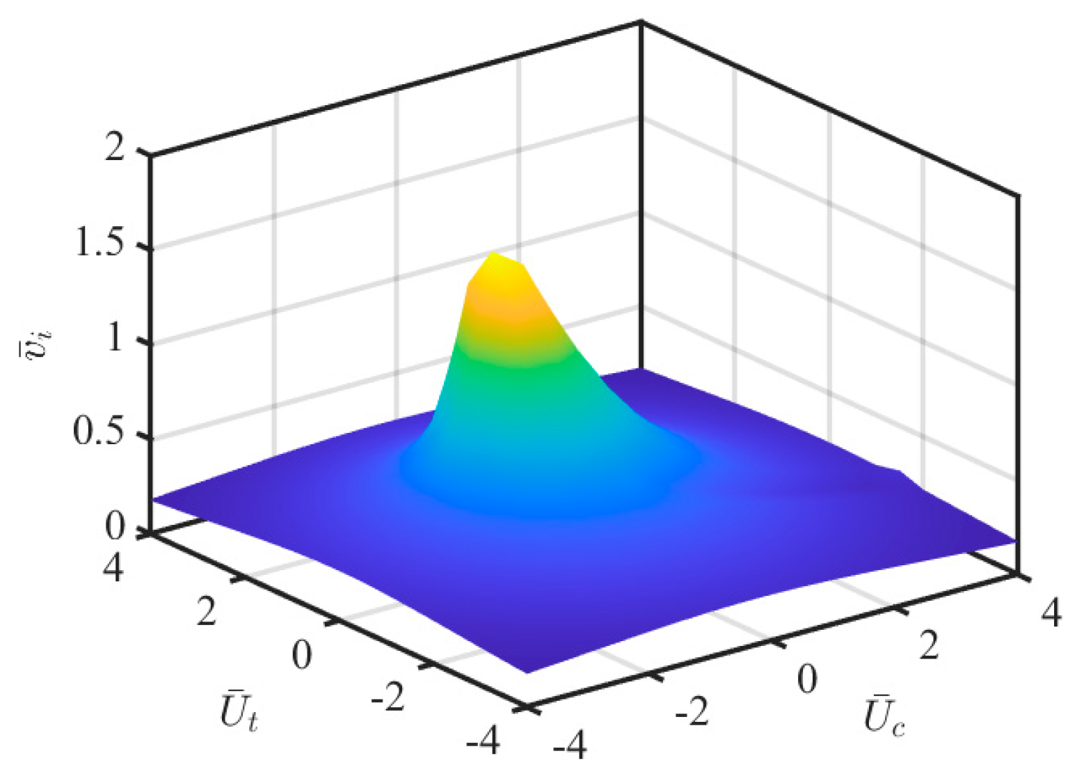
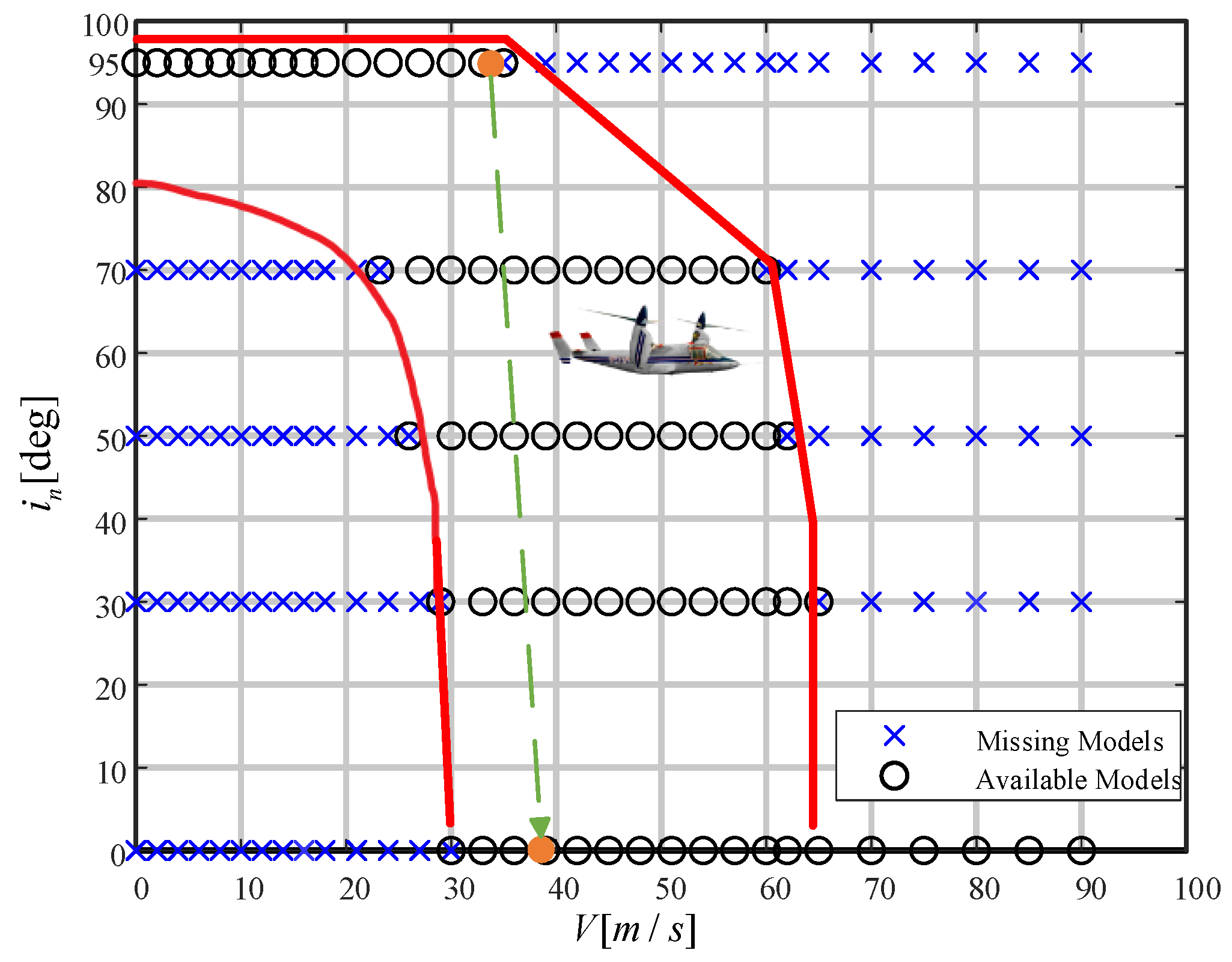
In tilt-transition mode, the tiltrotor aircraft experiences continuous variations in nacelle tilt angle and flight velocity, which lead to significant nonlinear coupling between rotor aerodynamics and body-axis force components. Additionally, the aerodynamic forces acting on the body change drastically, influencing the flight states of tiltrotor aircraft. Thus, these dynamic interactions necessitate a rigorous steady-state analysis to quantify equilibrium conditions throughout the transition corridor.

During the transition phase of flight, the vertical velocity of the aircraft remains relatively low, while its horizontal velocity is higher. At this stage, the thrust generated by the rotor becomes the primary source of both speed and lift. Therefore, the angle of attack and the nacelle angle play a critical role in aircraft control. As the flight speed increases, the aerodynamic forces and moments acting on the fuselage also increase. Since the angle of attack directly influences these aerodynamic forces and moments, it is essential to control the angle of attack precisely when the aerodynamic force is the main source of lift. To mitigate transient disturbances during trimming, the angle of attack is constrained to 0°. Subsequently, different nacelle angles and rotor-generated lift values are selected to trim the tiltrotor aircraft. The resulting trim points are shown in

Table 1. Tilt-transition mode trim points for tiltrotor aircraft.

$i_n (°)$	$T (\mathrm{kg})$	$\overline{S}$	$\dot{x} (\mathrm{m}/\mathrm{s})$	$w (\mathrm{m}/\mathrm{s})$	$u (\mathrm{m}/\mathrm{s})$	$\theta (°)$
0	2000.4117	−0.30718	39.0468	0.54598	39.0461	0.0060427
0	3000.0496	−0.04488	43.9811	−1.9956	43.9358	−0.04539
0	4799.7321	0.19269	51.1602	−4.718	50.9422	−0.092351
0	7000.0007	0.33824	58.3998	−7.1048	57.966	−0.12196
10	1600.5173	−0.48144	36.395	1.5068	36.3638	0.041413
30	1700.7331	−0.55907	34.9736	2.0532	34.9132	0.058742
50	2500.2169	−0.55059	34.239	1.9859	34.1981	0.058005
70	5758.8306	−0.41916	33.1861	1.0851	33.2289	0.032644
90	5895.2422	−0.5724	1.07 × 10−9	−9.67 × 10−1	9.67 × 10−1	−0.11521
95	6500.0262	−0.91267	2.9334	−0.21808	2.9253	−0.074411

where $\overline{S}=s/s_{\max }$, and $s$ denotes the longitudinal stick displacement.

, and the equilibrium points satisfy the following equation:

$$f(x_0,u_0)=0$$

(17)

where $x_0$ represents the trimmed state vector, and $u_0$ represents the trimmed control vector. The validated trim points demonstrate monotonic convergence across the transition envelope.

The data from the table indicate that when $i_n={90}^{\circ }$, the aircraft achieves hovering equilibrium with $w\approx 0\mathrm{m}/\mathrm{s}$ and $u\approx 0\mathrm{m}/\mathrm{s}$, which is consistent with rotor-dominated vertical thrust. The data are used to construct a two-dimensional grid map that quantitatively relates flight speed to nacelle tilt angle, as illustrated in Figure 7. Additionally, the grid points outside the transition corridor represent trimmed states at extreme velocities. The monotonic convergence of trim points across $i_n\in [0^{\circ },{90}^{\circ }]$ provides critical reference states for controller synthesis, particularly in addressing hybrid aerodynamic dominance during mode transitions.

4. Design of the Controller

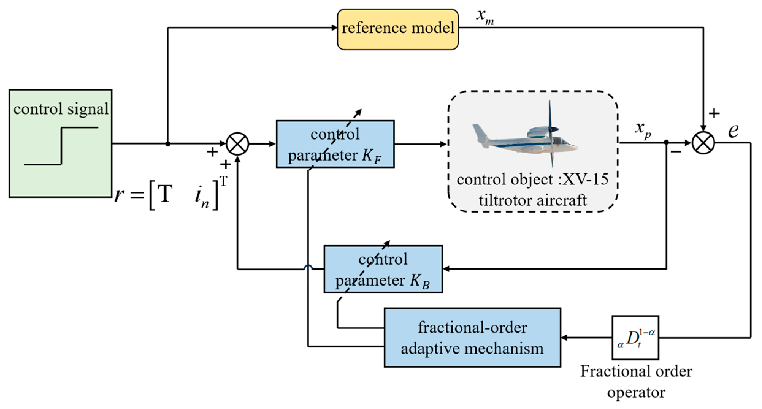
In this paper, the equilibrium states tabulated in Table 1 are identified as linearization baselines, and a fractional-order control strategy is proposed for the tiltrotor aircraft, as illustrated in Figure 8. The control input $r$ is processed through a feedforward gain matrix $K_F$ to generate an initial control signal. Subsequently, the plant output $x_p$ is compared with the reference model output $x_m$, generating a tracking error $e=x_m-x_p$, which is modulated by a fractional-order operator and adjusted via feedback gain.

At the equilibrium points $(x_0,u_0)$, the nonlinear dynamics are linearized as

$$\left\{\begin{array}{l}\dot{x}=A\Delta x+B\Delta u\\ y=\Delta x\end{array}\right.$$

(18)

where $A={\displaystyle \frac{\partial f}{\partial x}}{|}_{x=x_0}$, $B={\displaystyle \frac{\partial f}{\partial u}}{|}_{u=u_0}$, $\dot{x}=\Delta \dot{x}$, $\Delta x=x-x_0$, and $\Delta u=u-u_0$. To address residual nonlinearities $f\left(x_0,u_0\right)\ne 0$, a corrective $G$ function is introduced, and the equation can be further rewritten as [33]

$$\left\{\begin{array}{l}{\dot{x}}_p=A_p{x}_p+B_{p}u+G\\ y=C_p{x}_p\end{array}\right.$$

(19)

where $B_p=B$, $A_p=A$, and $C_p\in R^{7\times 7}$. The reference model for the FO-MRAC system is formulated as

$${\dot{x}}_m=A_m{x}_m+B_{m}r+G$$

(20)

where $r=u$, $A_m$, and $B_m$ are system matrices with $A_m\in R^{n\times n}$, $B_m\in R^{n\times m}$. The state tracking error is defined as

$$e=x_m-x_p$$

(21)

To ensure effective tracking, the control law is designed as

$$u=K_F\left(K_B{x}_p+r\right)$$

(22)

where $K_F$ represents the feedforward gain matrix, and $K_B$ represents the feedback gain matrix, acting as the bridge between the adaptive mechanism and the control law. Based on prior Equations (19) and (20), the state equation of the tracking error can be further derived as

$$\dot{e}=A_{m}e+\left[A_m-A_p-B_p{K}_F{K}_B\right]x_p+\left[B_m-B_p{K}_F\right]r$$

(23)

Assuming the reference model and system satisfy the completely matchable condition [34], there exist matrices $K_F^{\ast }$ and $K_B^{\ast }$ such that $A_p+B_p{K}_F^{\ast }{K}_B^{\ast }=A_m$ and $B_p{K}_F^{\ast }=B_m$. Substituting the matrices into the error dynamics Equation (23), we obtain

$$\dot{e}=A_{m}e+B_m\left[{\tilde{K}}_B{x}_p+{\tilde{K}}_{Fi}\widehat{r}\right]$$

(24)

where ${\tilde{K}}_{Fi}=K_F^{-1}-K_F^{\ast -1}$, ${\tilde{K}}_F=K_F^{\ast }-K_F$, and ${\tilde{K}}_B=K_B^{\ast }-K_B$ denote the parameter adaptation errors. To analyze the stability of the closed-loop system, the Lyapunov function is constructed as

$$V={\displaystyle \frac{1}{2}}{\left({}_{a}D_t^{1-\alpha }e\right)}^{\mathrm{T}}P\left({}_{a}D_t^{1-\alpha }e\right)+{\displaystyle \frac{1}{2}}\mathrm{tr}\left[{\left({}_{a}D_t^{1-\alpha }{\tilde{K}}_B\right)}^{\mathrm{T}}{\Gamma }_B^{-1}{\tilde{K}}_B\right]+{\displaystyle \frac{1}{2}}\mathrm{tr}\left[{\left({}_{a}D_t^{1-\alpha }{\tilde{K}}_{Fi}\right)}^{\mathrm{T}}{\Gamma }_F^{-1}{\tilde{K}}_{Fi}\right]$$

(25)

where $P>0$, ${\Gamma }_B>0$, ${\Gamma }_F>0$, and $0<\alpha \le 1$ are parameters to be designed. Furthermore, the operator $\mathrm{tr}(A)$ is the trace operation if $A\in R^{n\times n}$. Taking the fractional-order time derivative of $V$, the system stability conditions can be further evaluated:

$${}_{a}D_t^{\alpha }V={\displaystyle \frac{1}{2}}\left[{\left({}_{a}D_t^{1-\alpha }e\right)}^{\mathrm{T}}P\dot{e}+{\dot{e}}^{\mathrm{T}}P\left({}_{a}D_t^{1-\alpha }e\right)\right]+\mathrm{tr}\left({\dot{\tilde{K}}}_B^{\mathrm{T}}{\Gamma }_B^{-1}{\tilde{K}}_B\right)+\mathrm{tr}\left({\dot{\tilde{K}}}_{Fi}^{\mathrm{T}}{\Gamma }_F^{-1}{\tilde{K}}_{Fi}\right)$$

(26)

According to Equation (24), the derivation can be continued as follows:

$${}_{a}D_t^{\alpha }V={\displaystyle \frac{1}{2}}{e}^{\mathrm{T}}\left(P{A}_m+A_m^{\mathrm{T}}P\right)\left({}_{a}D_t^{1-\alpha }e\right)+\mathrm{tr}\left\{\left[{\left({}_{a}D_t^{1-\alpha }e\right)}^{\mathrm{T}}P{B}_m{x}_p+{\dot{\tilde{K}}}_B^{\mathrm{T}}{\Gamma }_B^{-1}\right]{\tilde{K}}_B\right\}+\mathrm{tr}\left\{\left[{\left({}_{a}D_t^{1-\alpha }e\right)}^{\mathrm{T}}P{B}_m\widehat{r}+{\dot{\tilde{K}}}_{Fi}^{\mathrm{T}}{\Gamma }_F^{-1}\right]{\tilde{K}}_{Fi}\right\}$$

(27)

The adaptation laws are defined as

$$\begin{array}{r}\left[{\left({}_{a}D_t^{1-\alpha }e\right)}^{\mathrm{T}}P{B}_m{x}_p+{\dot{\tilde{K}}}_B^{\mathrm{T}}{\Gamma }_B^{-1}\right]{\tilde{K}}_B=0\\ \left[{\left({}_{a}D_t^{1-\alpha }e\right)}^{\mathrm{T}}P{B}_m\widehat{r}+{\dot{\tilde{K}}}_{Fi}^{\mathrm{T}}{\Gamma }_F^{-1}\right]{\tilde{K}}_{Fi}=0\end{array}$$

(28)

Since $A_m$ is a positive-definite matrix, there exist positive-definite matrices $P$ and $Q$ such that $P{A}_m+A_m^{T}P=-Q$, and thus, ${}_{a}D_t^{\alpha }V<0$ [35]. The above-mentioned adaptation laws can ensure that the fractional-order closed-loop system is globally asymptotically stable. The parameter adaptation laws are formulated as

$$\left\{\begin{array}{l}-{\dot{K}}_B={\dot{\tilde{K}}}_B=-{\Gamma }_B^{-1}{B}_m^{\mathrm{T}}P\left({}_{a}D_t^{1-\alpha }e\right)x_p^{\mathrm{T}}\\ -{\dot{K}}_{Fi}={\dot{\tilde{K}}}_{Fi}=-{\Gamma }_F^{-1}{B}_m^{\mathrm{T}}P\left({}_{a}D_t^{1-\alpha }e\right){\widehat{r}}^{\mathrm{T}}\end{array}\right.$$

(29)

In terms of Equation (29) and ${\tilde{K}}_{Fi}=K_F^{-1}-K_F^{\ast -1}$, the parameter ${\dot{K}}_F$ can be obtained as

$${\dot{K}}_F=-K_F{\dot{K}}_{Fi}{K}_F=-K_F{\Gamma }_F^{-1}{B}_m^{\mathrm{T}}P\left({}_{a}D_t^{1-\alpha }e\right){\left(K_B{x}_p+r\right)}^{\mathrm{T}}{K}_F^{\mathrm{T}}{K}_F$$

(30)

According to Equations (22), (29) and (30), the adaptive controller is obtained as

$$\left\{\begin{array}{l}u=K_F\left(K_B{x}_p+r\right)\\ {\dot{K}}_F=-K_F{\Gamma }_F^{-1}{B}_m^{\mathrm{T}}P\left({}_{a}D_t^{1-\alpha }e\right){\left(K_B{x}_p+r\right)}^{\mathrm{T}}{K}_F^{\mathrm{T}}{K}_F\\ {\dot{K}}_B={\Gamma }_B^{-1}{B}_m^{\mathrm{T}}P\left({}_{a}D_t^{1-\alpha }e\right)x_p^{\mathrm{T}}\end{array}\right.$$

(31)

When there are disturbances in the parameters, assume the external disturbance $d(t)$ satisfies $‖d(t)‖\le d_{\max }$, and consider the following modified adaptation law:

$${\dot{K}}_B={\Gamma }_B^{-1}\left(B_m^{\mathrm{T}}P({}_{\alpha }D_t^{1-\alpha }e)x_p^{\mathrm{T}}-{\sigma }_B{K}_B\right)$$

(32)

which is also applicable to $K_F$, and the auxiliary Lyapunov function is introduced later.

$$V_1=V+{\displaystyle \frac{1}{2}}\mathrm{tr}\left({\tilde{K}}_B^T{\sigma }_B^{-1}{\tilde{K}}_B\right)$$

(33)

where $V$ is the original Lyapunov function. Take the derivative of $V_1$ and substitute ${\dot{K}}_B$:

$${\dot{V}}_1=\dot{V}-\mathrm{tr}\left({\Gamma }_B^{-1}{x}_p{}_{a}D_t^{1-\alpha }{e}^T{P}^T{B}_m{\sigma }_B^{-1}{\tilde{K}}_B\right)+\mathrm{tr}\left({\Gamma }_B^{-1}{K}_B^T{\tilde{K}}_B\right)$$

(34)

According to the complete-square inequality, the ${\dot{V}}_1$ can be further rewritten as

$${\dot{V}}_1\le -\lambda {‖e‖}^2+{\displaystyle \frac{{d^2}_{\max }}{4{\lambda }_{\min }({\sigma }_B{\Gamma }_B)}}$$

(35)

This shows that ${\dot{V}}_1$ is bounded. Furthermore, combined with Barbalat’s lemma [36], we have

$$‖{\tilde{K}}_B‖\le {\displaystyle \frac{{\Gamma }_B{d}_{\max }}{{\sigma }_B}}, ‖{\tilde{K}}_F‖\le {\displaystyle \frac{{\Gamma }_F{d}_{\max }}{{\sigma }_F}}$$

(36)

5. Hardware-in-the-Loop Validation

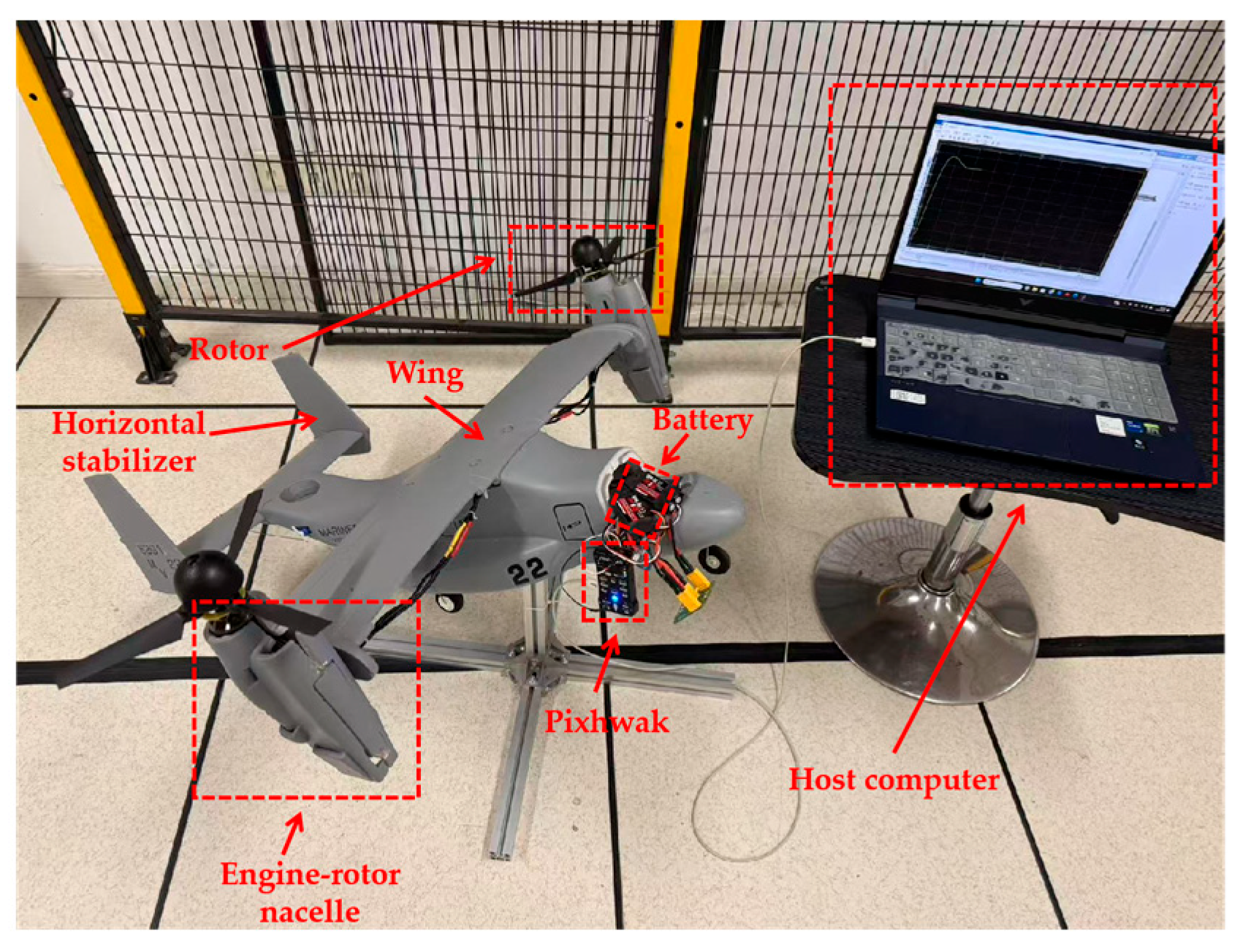
To validate the effectiveness of the control law, a hardware-in-the-loop (HIL) platform is established. We simulated the model of the tilting rotor aircraft with a fixed time step on the PC to ensure its high fidelity. The simulation system realizes two-way communication with the Pixhawk flight control hardware through the MAVLink HIL protocol, ports 14540/14550, and a message frequency of 200 Hz, ensuring strict time synchronization between the controller and the simulation model. The PX4 firmware integrates a sensor simulation module internally, including a barometer, magnetometer, and gyroscope, etc., enabling Pixhawk to receive perception data consistent with those of actual aircraft. The actuator commands output by Pixhawk are received by Simulink and sent to the control plane or motor via the serial port, forming a complete feedback loop. Flight control laws are deployed to Pixhawk via PX4 firmware for real-time operation. Figure 9 and Figure 10 clearly show the closed-loop structure, USB communication path, MAVLink protocol interface, and sensor and actuator simulation module, thereby more clearly demonstrating the structural integrity and modeling fidelity of the HIL system.

To conduct the validation, the transition process is designed by selecting two stable flight states within the operational envelope of the tiltrotor aircraft, as depicted in Figure 11. As shown in Figure 11, the transition maneuver is simulated starting from an initial state of $\left(i_n,V\right)=\left({95}^{\circ },35.6\mathrm{m}/\mathrm{s}\right)$ and reaching a final state of $\left(i_n,V\right)=\left(0^{\circ },38.7\mathrm{m}/\mathrm{s}\right)$.

5.1. Flight States Verification of the Integer-Order System at a Single Stable Point

To demonstrate that the tiltrotor aircraft states do not converge effectively under a uniform set of control parameters, we choose two states, $\left(i_n,V\right)=\left({75}^{\circ },37.6\mathrm{m}/\mathrm{s}\right)$ and $\left(i_n,V\right)=\left(0^{\circ },41.1\mathrm{m}/\mathrm{s}\right)$. Two distinct control parameters are provided in

Table 2. First group of control parameters.

$K_A$	$u$	$w$	$q$	$\theta$
$T$	1849.0265	514.0925	11,242.4676	70,580.0848
$i_n$	0.0900	0.0529	1.9046	0.7137

and

Table 3. The second group of control parameters.

$K_B$	$u$	$w$	$q$	$\theta$
$T$	166.6076	1453.3844	22,717.2814	51,814.6621
$i_n$	0.1418	0.0516	0.3167	−0.0710

, respectively.

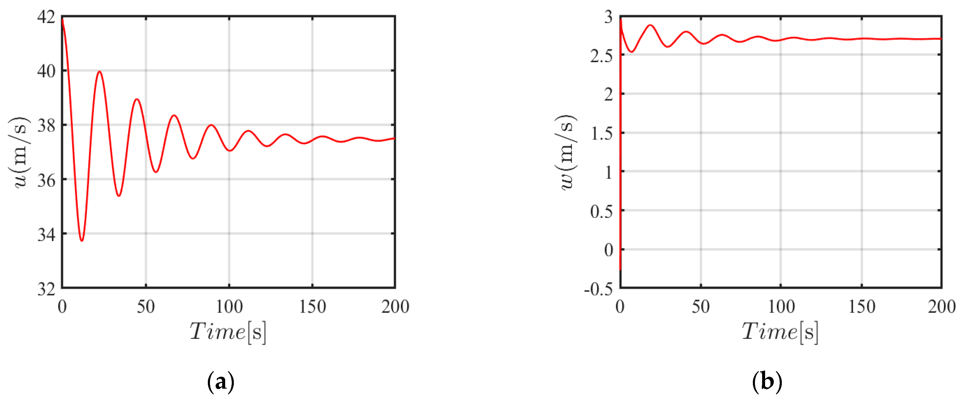
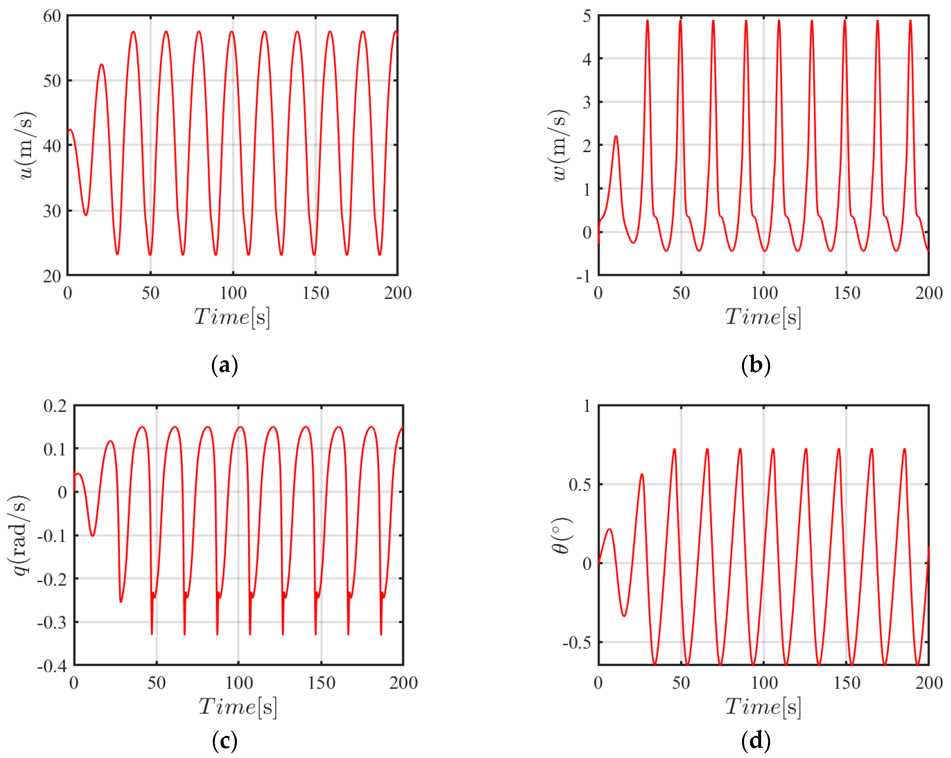
As shown in Figure 12, under the initial flight condition, the dynamic response of a step input signal was achieved by using the first set of control parameters. Specifically, the responses of the horizontal speed, the vertical velocity, the pitch angular velocity, and the pitch angle are depicted in Figure 12a–d, respectively. As shown in Figure 12, the closed-loop system is stable under the initial flight condition. Furthermore, the response of a step input signal under the final condition is shown in Figure 13. 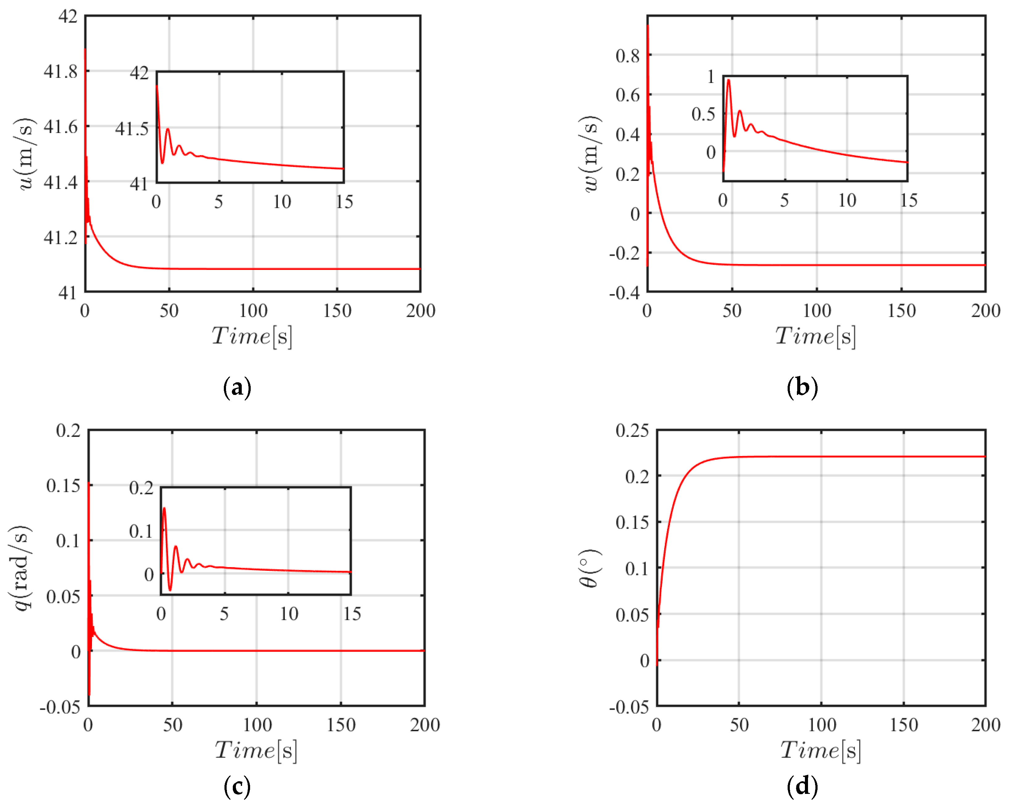As shown in Figure 13, the closed-loop system is unstable under the final condition. Such an unstable phenomenon could be attributed to parameter mismatches or insufficient gain tuning in the controller design under the initial flight condition, which cannot meet the control requirement in the later stages of flight. To address this limitation, a second group of control parameters was developed through re-tuning the controller gains in terms of Equation (30). The dynamic response under the re-tuning of the controller gains is shown in Figure 14. As shown in Figure 14, the stability of the closed-loop system is achieved either under the initial flight condition or under the final condition, which confirms the effectiveness of the proposed gain tuning regulation (30).

5.2. Verification of Tiltrotor Aircraft Transition Process

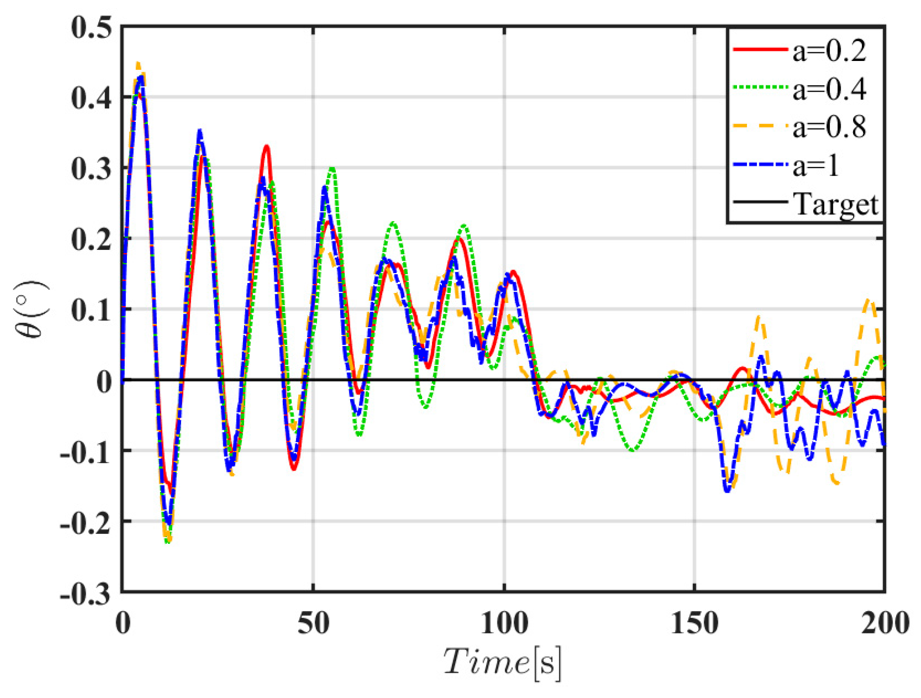
FO-MRAC has been developed to ensure a smooth transition between the two states. In order to verify how to select the appropriate fractional order $\alpha$, the pitch angle $\theta$ is taken as the research object to study the influence on the error size under different fractional orders. Select different fractional orders: $\alpha =0.2$, $\alpha =0.4$, $\alpha =0.8$, $\alpha =1$.

As shown in Figure 15, when the fractional-order exponent is $0<\alpha \le 1$, selecting a fractional-order exponent can reduce the error and enhance the stability. Therefore, an appropriate fractional-order exponent of $\alpha =0.2$ is selected. To illustrate the superiority of the proposed method, the MRAC method and a conventional linear controller (CLM) are also designed with the same parameters.

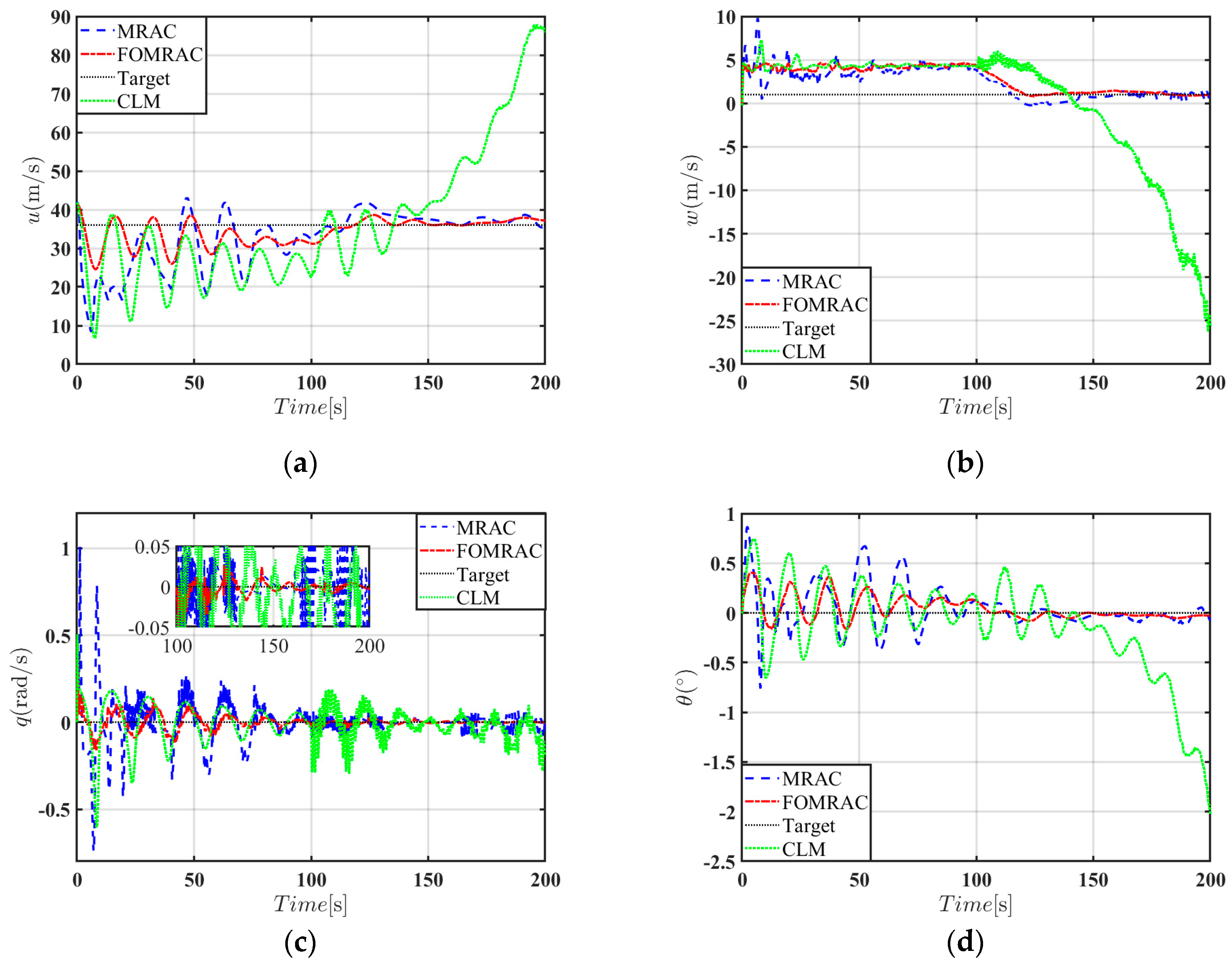
As shown in Figure 16, the transition process of the tiltrotor aircraft begins at 100 s. The proposed FO-MRAC control method exhibits a notably faster dynamic response, achieving an average regulation time of 18.65 s, compared to 36.92 s for the conventional MRAC. The comparison between the two methods shows that the efficiency has increased by 50.51%. In terms of forward velocity tracking, the disturbance error under integer-order control ranges from 0% to 4.12%, whereas the FO-MRAC reduces this range to 0–1.27%, demonstrating its superior capability in suppressing both overshoot and steady-state error while preserving overall stability. Moreover, the reduced oscillation amplitude during the transition further confirms the enhanced transient performance and steady-state behavior of the FO-MRAC scheme. These quantitative indicators fully verify the robustness and effectiveness of this control strategy in dealing with complex flight state transitions.

6. Conclusions

By investigating four key components, such as rotors, wings, fuselage, and horizontal tail, motion models are established to accurately capture the forces and moments acting on these key parts. Based on the models, the nonlinear simulation model is subsequently linearized to obtain the equilibrium points of the aircraft under various flight modes, facilitating the construction of the stable flight envelope. To address the system uncertainties and external disturbances, an FO-MRAC strategy is introduced. Leveraging the flexibility of fractional-order operators, the strategy enables precise parameter tuning and exceptional disturbance rejection capabilities, which ensures favorable flight stability. Considering that the tilting transition process has significant nonlinear and time-varying characteristics, further research will be carried out in the future focusing on the theoretical completeness and engineering practicability of the controller, mainly including factors such as non-modeling dynamics, bounded parameter disturbances, and actuator delays, to conduct research on uncertainty modeling and compensation mechanisms. Combining the state observer or neural network approximation method, a nonlinear full-envelope controller is constructed to adapt to severe flight maneuvers and complex working conditions.

References

1. Rollet, P. RHILP-a major step for european knowledge in tilt-rotor aeromechanics and flight dynamics. Air Space Eur. 2001, 3, 152–154. [Google Scholar] [CrossRef]
2. Hegde, N.T.; George, V.I.; Nayak, C.G.; Kumar, K. Design, Dynamic Modelling and Control of Tilt-Rotor UAVs: A Review. Int. J. Intell. Unmanned Syst. 2019, 8, 143–161. [Google Scholar] [CrossRef]
3. Alli, P. Erica: The European Tiltrotor. Design and Critical Technology Projects. In Proceedings of the AIAA International Air and Space Symposium and Exposition: The Next 100 Years, Dayton, OH, USA, 14 July 2003; American Institute of Aeronautics and Astronautics: Reston, VA, USA, 2003. [Google Scholar]
4. Liu, N.; Wang, Y.; Zhao, J.; Chen, X.; He, X.; Wu, K. A new inclining flight mode and oblique takeoff technique for a tiltrotor aircraft. Aerosp. Sci. Technol. 2023, 139, 108370. [Google Scholar] [CrossRef]
5. Lu, K.; Tian, H.; Zhen, P.; Lu, S.; Chen, R. Conversion Flight Control for Tiltrotor Aircraft via Active Disturbance Rejection Control. Aerospace 2022, 9, 155. [Google Scholar] [CrossRef]
6. Rohr, D.; Studiger, M.; Stastny, T.; Lawrance, N.N.R.J.; Siegwart, R. Nonlinear Model Predictive Velocity Control of a VTOL Tiltwing UAV. IEEE Robot. Autom. Lett. 2021, 6, 5776–5783. [Google Scholar] [CrossRef]
7. Zheng, P.; Tan, X.K.; Kocer, B.B.; Yang, E.D.; Kovac, M. TiltDrone: A Fully-Actuated Tilting Quadrotor Platform. IEEE Robot. Autom. Lett. 2020, 5, 6845–6852. [Google Scholar] [CrossRef]
8. Su, W.; Qu, S.; Zhu, G.; Swei, S.S.M.; Hashimoto, M.; Zheng, T. Modeling and control of a class of urban air mobility tiltrotor aircraft. Aerosp. Sci. Technol. 2022, 124, 107561. [Google Scholar] [CrossRef]
9. Tischler, M.B.; Leung, J.G.M.; Dugan, D.C. Identification and Verification of Frequency-Domain Models for XV-15 Tilt-Rotor Aircraft Dynamics in cruising flight. J. Guid. Control. Dyn. 1984, 9, 446–453. [Google Scholar] [CrossRef]
10. Tischler, M.B. Frequency-Response Identification of XV-15 Tilt-Rotor Aircraft Dynamics; Stanford University: Redwood City, CA, USA, 1987. [Google Scholar]
11. Liang, Z.; Fan, L.; Wen, G.; Xu, Z. Design, Modeling, and Control of a Composite Tilt-Rotor Unmanned Aerial Vehicle. Drones 2024, 8, 102. [Google Scholar] [CrossRef]
12. Juhasz, O.; Celi, R.; Tischler, M. Flight Dynamics Simulation Modeling of a Large Flexible Tiltrotor Aircraft. J. Am. Helicopter Soc. 2022, 67, 1–16. [Google Scholar] [CrossRef]
13. Lu, K.; Liu, C.; Li, C.; Chen, R. Flight Dynamics Modeling and Dynamic Stability Analysis of Tilt-Rotor Aircraft. Int. J. Aerosp. Eng. 2019, 2019, 1–15. [Google Scholar] [CrossRef]
14. Henkenjohann, M.; Nolte, U.; Sion, F.; Henke, C.; Trachtler, A. Parameter Tuning Approach for Incremental Nonlinear Dynamic Inversion-Based Flight Controllers. Actuators 2024, 13, 187. [Google Scholar] [CrossRef]
15. Zhang, J.; Sun, L.; Qu, X.; Wang, L. Time-Varying Linear Control for Tiltrotor Aircraft. Chin. J. Aeronaut. 2018, 31, 632–642. [Google Scholar] [CrossRef]
16. Liu, H.; Wang, N.; Zhang, Z.; Yin, H. Agile and Precise Attitude Control of Tiltrotor Aircraft in Transition Flight. IEEE Trans. Intell. Veh. 2024, 9, 787–798. [Google Scholar] [CrossRef]
17. Wang, Z.; Gong, Z.; Chen, Y.; Sun, M.; Xu, J. Practical control implementation of tri-tiltRotor flying wing unmanned aerial vehicles based upon active disturbance rejection control. Proc. Inst. Mech. Eng. Part G-J. Aerosp. Eng. 2020, 234, 943–960. [Google Scholar] [CrossRef]
18. Bauersfeld, L.; Spannagl, L.; Ducard, G.J.J.; Onder, C.H. MPC Flight Control for a Tilt-Rotor VTOL Aircraft. IEEE Trans. Aerosp. Electron. Syst. 2021, 57, 2395–2409. [Google Scholar] [CrossRef]
19. Luo, L.; Xu, S.; Su, C.; Xie, M.; Li, J. Fixed-time composite observer-based adaptive recursive sliding mode control for tiltrotor UAV attitude tracking. Nonlinear Dyn. 2025, 113, 1–26. [Google Scholar] [CrossRef]
20. Yang, G. State filtered disturbance rejection control. Nonlinear Dyn. 2025, 113, 6739–6755. [Google Scholar] [CrossRef]
21. Yang, G.; Yao, J. Multilayer neurocontrol of high-order uncertain nonlinear systems with active disturbance rejection. Int. J. Robust Nonlinear Control 2024, 34, 2972–2987. [Google Scholar] [CrossRef]
22. Liu, N.; Cai, Z.; Zhao, J.; Wang, Y. Predictor-based model reference adaptive roll and yaw control of a quad-tiltrotor UAV. Chin. J. Aeronaut. 2020, 33, 282–295. [Google Scholar] [CrossRef]
23. Wen, J.; Song, Y.; Wang, H.; Han, D.; Yang, C. Hybrid Adaptive Control for Tiltrotor Aircraft Flight Control Law Reconfiguration. Aerospace 2023, 10, 1001. [Google Scholar] [CrossRef]
24. Shen, S.; Xu, J.; Chen, P.; Xia, Q. Adaptive Neural Network Extended State Observer-Based Finite-Time Convergent Sliding Mode Control for a Quad Tiltrotor UAV. IEEE Trans. Aerosp. Electron. Syst. 2023, 59, 6360–6373. [Google Scholar] [CrossRef]
25. Lu, E.; Li, W.; Jiang, S.; Liu, Y. Anti-Disturbance Speed Control of Permanent Magnet Synchronous Motor Based on Fractional Order Sliding Mode Load Observer. IEEE Access 2024, 12, 71716–71732. [Google Scholar] [CrossRef]
26. Zhang, X.; Zhag, X.; Li, M.; Deng, X.; Du, L. Fractional-order electric spring based on fuzzy PIλDμ adaptive control. J. Power Electron. 2025, 25, 1–12. [Google Scholar] [CrossRef]
27. Carlson, E.B. Optimal Tiltrotor Aircraft Operations During Power Failure; University of Minnesota: Minneapolis, MN, USA, 1999. [Google Scholar]
28. Ghoreyshi, M.; Jirásek, A.; Cummings, R.M. Reduced order unsteady aerodynamic modeling for stability and control analysis using computational fluid dynamics. Prog. Aerosp. Sci. 2014, 71, 167–217. [Google Scholar] [CrossRef]
29. Zhao, G.; Cui, Z.; Zhao, Q.; Chen, X.; Li, P. Investigations on Trimming Strategy and Unsteady Aerodynamic Characteristics of Tiltrotor in Conversion Procedure. Aerospace 2024, 11, 632. [Google Scholar] [CrossRef]
30. Johnson, W. Helicpoter Theory; Courier Corporation: Chelmsford, MA, USA, 1980; pp. 282–283. [Google Scholar]
31. Stepniewski, W.Z.; Keys, C.N. Rotary-Wing Aerodynamics; Courier Corporation: Chelmsford, MA, USA, 1984. [Google Scholar]
32. Johnson, W. Helicopter Optimal Descent and Landing after Power Loss; NASA TM 73244, NASA: Washington, DC, USA, 1977.
33. Yang, X.; Hu, X.; Ye, H.; Liu, W.; Shen, H. Fraction-order MRAC Method Based Fault Tolerant Control for Plant Protection UAV with Actuator Failure and Uncertainty. Int. J. Control. Autom. Syst. 2023, 21, 2623–2633. [Google Scholar] [CrossRef]
34. Song, G.; Tao, G. Partial-state feedback multivariable MRAC and reduced-order designs. Automatica 2021, 129, 109622. [Google Scholar] [CrossRef]
35. Sun, H.; Li, J.; Wang, R.; Yang, K. Attitude Control of the Quadrotor UAV with Mismatched Disturbances Based on the Fractional-Order Sliding Mode and Backstepping Control Subject to Actuator Faults. Fractal Fract. 2023, 7, 227. [Google Scholar] [CrossRef]
36. Chaudhary, K.S.; Kumar, N. A New Hybrid Control Scheme for Tracking Control Problem of AUVs with System Uncertainties and External Disruptions. J. Field Robot. 2025, 42, 716–741. [Google Scholar] [CrossRef]
Figure 2. Lift and drag in body components.
Machines 13 00439 g002
Figure 3. The aerodynamic fitting curves against XV-15 data.
Machines 13 00439 g003
Figure 4. Wing affected by the free stream and slipstream.
Machines 13 00439 g004
Figure 5. Wing and horizontal stabilizer fitting results with XV-15 data. (a) The fitting result of the lift coefficient in the wing; (b) The fitting result of the drag coefficient in the wing; (c) The fitting result of the total aerodynamic moment in the wing; (d) The fitting result of the lift coefficient in the horizontal stabilizer.
Machines 13 00439 g005
Figure 6. Normalized induced velocity.
Machines 13 00439 g006
Figure 7. The flight envelope of the tiltrotor aircraft.
Machines 13 00439 g007
Figure 8. The fractional-order model refers to the adaptive schematic diagram.
Machines 13 00439 g008
Figure 9. Structure diagram of the HIL simulation platform.
Machines 13 00439 g009
Figure 10. Verification platform.
Machines 13 00439 g010
Figure 11. Tiltrotor aircraft flight transition process diagram.
Machines 13 00439 g011
Figure 12. System response at the initial flight condition using the first parameter. (a) The response curve of horizontal speed under the step-response signal; (b) The response curve of vertical speed under the step-response signal; (c) The response curve of pitch angular velocity under the step-response signal; (d) The response curve of the pitch angle under the step-response signal.
Machines 13 00439 g012aMachines 13 00439 g012b
Figure 13. System response at the final equilibrium state using the first parameters. (a) The response curve of horizontal speed under the step-response signal; (b) The response curve of vertical speed under the step-response signal; (c) The response curve of pitch angular velocity under the step-response signal; (d) The response curve of the pitch angle under the step-response signal.
Machines 13 00439 g013
Figure 14. System response at the final equilibrium state using the second parameter. (a) The response curve of horizontal speed under the step-response signal; (b) The response curve of the pitch angle under the step-response signal; (c) The response curve of pitch angular velocity under the step-response signal; (d) The response curve of the pitch angle under the step-response signal.
Machines 13 00439 g014
Figure 15. Comparative simulation of each order of forward velocity.
Machines 13 00439 g015
Figure 16. Transition process response curves. (a) The impact of different control methods on horizontal speed; (b) The impact of different control methods on vertical speed; (c) The impact of different control methods on pitch angular velocity; (d) The impact of different control methods on pitch angle.
Machines 13 00439 g016