Article

Self-Regulating Fuzzy-LQR Control of an Inverted Pendulum System via Adaptive Hyperbolic Error Modulation

1
Department of Electrical Engineering, National University of Computer and Emerging Sciences, Lahore 54770, Pakistan
2
School of Digital and Physical Sciences, Faculty of Science and Engineering, University of Hull, Hull HU6 7RX, UK
3
Department of Electrical and Electronic Engineering, College of Engineering, University of Jeddah, Jeddah 23890, Saudi Arabia
*
Author to whom correspondence should be addressed.
Machines 2025, 13(10), 939; https://doi.org/10.3390/machines13100939 (registering DOI)
Submission received: 9 August 2025 / Revised: 23 September 2025 / Accepted: 10 October 2025 / Published: 12 October 2025
(This article belongs to the Special Issue Mechatronic Systems: Developments and Applications)

Abstract

This study introduces an innovative self-regulating intelligent optimal balancing control framework for inverted pendulum-type mechatronic platforms, designed to enhance reference tracking accuracy and improve disturbance rejection capability. The control procedure is synthesized by synergistically integrating a baseline Linear Quadratic Regulator (LQR) with a fuzzy controller via a customized linear decomposition function (LDF). The LDF dissociates and transforms the LQR control law into compounded state tracking error and tracking error derivative variables that are eventually used to drive the fuzzy controller. The principal contribution of this study lies in the adaptive modulation of these compounded variables using reconfigurable tangent hyperbolic functions driven by the cubic power of the error signals. This nonlinear preprocessing of the input variables selectively amplifies large errors while attenuating small ones, thereby improving robustness and reducing oscillations. Moreover, a model-free online self-tuning law dynamically adjusts the variation rates of the hyperbolic functions through dissipative and anti-dissipative terms of the state errors, enabling autonomous reconfiguration of the nonlinear preprocessing layer. This dual-level adaptation enhances the flexibility and resilience of the controller under perturbations. The robustness of the designed controller is substantiated via tailored experimental trials conducted on the Quanser rotary pendulum platform. Comparative results show that the prescribed scheme reduces pendulum angle variance by 41.8%, arm position variance by 34.6%, and average control energy by 28.3% relative to the baseline LQR, while outperforming conventional fuzzy-LQR by similar margins. These results show that the prescribed controller significantly enhances disturbance rejection and tracking accuracy, thereby offering a numerically superior control of inverted pendulum systems.

1. Introduction

The inverted pendulum (IP) system is a well-known benchmark problem in control theory that has been extensively researched because of its nonlinear dynamics, underactuated configuration, and inherent kinematic instability [1]. Their balancing control is not just a theoretical challenge but a practical necessity in many mechatronic applications, especially where systems are required to maintain postural stability even in the presence of environmental disturbances [2,3]. The IP system needs an agile control mechanism to actively maintain vertical balance because the bounded disturbances can cause it to collapse when upright [4]. The solution to this control problem is extensively used in a vast range of applications, ranging from attitude stabilization of drones to gait control in self-balancing scooters and walk-assistive robotic mechanisms [5,6]. Similarly to IPs, these systems are also required to maintain stability while moving or interacting with their surroundings, which makes efficient balancing control crucial [7]. The traditional control methods lack effectiveness against large disturbances owing to their nonlinear characteristics [8]. Therefore, devising control procedures that concurrently deal with nonlinearity and disturbances can substantially improve the performance and dependability of these systems in practical situations.

1.1. Literature Review

Different control techniques have been explored to achieve stabilization and trajectory tracking in IP systems [9]. Among them, the ubiquitous PID control is simple, easy to implement, and computationally efficient, making it suitable for small disturbances and linearized models [10]. However, it struggles with nonlinearities, requires manual tuning, and lacks robustness [11]. Fractional Order PID (FOPID) improves upon PID by offering finer tuning flexibility, better disturbance rejection, and improved robustness, but it introduces additional design complexity and higher computational demands [12]. It also introduces additional parameters, making the tuning process more complex [13]. Moreover, implementing non-integer-order integrals and derivatives is computationally intensive and often requires specialized numerical methods or approximation techniques for practical situations [14]. The sliding-mode control is highly robust to disturbances and uncertainties, ensuring finite-time convergence and strong stability, but it suffers from chattering, requires a precise model, and may need additional smoothing techniques [15,16]. The model predictive control effectively addresses constraints and nonlinearities by optimizing control actions over a prediction horizon [17]. However, it is computationally intensive, demands an accurate system model, and may introduce latency issues due to solving optimization problems at each step [18].
The Linear Quadratic Regulator (LQR) has been a dominant approach because of its optimal state feedback formulation and ability to minimize a quadratic cost function balancing control effort and state deviation [19]. LQR offers a computationally efficient solution for controlling an IP by deriving an optimal gain vector by solving the Riccati equation. The method ensures stability under nominal conditions and is extensively used in balancing underactuated robotic and mechatronic platforms [20]. However, standard LQR assumes a linearized state space model, which limits its performance in highly nonlinear regimes, model uncertainties, and external disturbances [21]. Its ineffectiveness against parametric variations has led researchers to explore hybrid approaches that integrate nonlinear and intelligent control techniques to enhance its performance [22].
Among the intelligent control systems, the neural controllers provide an agile control effort [23]. However, they require large training datasets and put a recursive computational burden on the digital computer [24]. The Fuzzy logic control (FLC) scheme, on the other hand, has also gained traction in controlling nonlinear and underactuated systems due to its ability to handle imprecise and uncertain information [25]. Unlike model-based controllers, the FLC relies on expert knowledge and heuristic rules, making it adaptable to complex dynamic environments [26]. They need an extensive set of qualitative rules in order to create a precise control model. The calibration of the associated membership functions is a laborious process, necessitating their hybridization with traditional controllers to achieve improved performance [27].
Comparative studies indicate that hybrid FLC approaches, such as Fuzzy-PID and Fuzzy-LQR, outperform standalone fuzzy controllers in terms of design flexibility and adaptability [28]. These hybrid schemes leverage the robustness of fuzzy inference while maintaining the inherent optimal characteristics of conventional controllers, leading to improved balance control and disturbance rejection. Recent studies on the hybridization of FLC and LQR controllers have shown that fuzzy inference can compensate for LQR’s sensitivity to parameter variations by adjusting the LQR’s control yield dynamically based on system states [29]. The use of nonlinear scaling functions for control signal modulation and adaptive gain scaling has been extensively studied in robotic applications [30]. Hyperbolic functions, particularly, have been utilized for their smooth saturation properties, allowing for adaptive gain adjustments and dynamic self-regulation of state error magnitudes without abrupt changes [31].
Recent developments in data-driven and machine learning-based control strategies have shown significant promise for rotary inverted pendulum systems [32,33]. Reinforcement learning (RL) techniques have been successfully applied to trajectory tracking and stabilization tasks in underactuated pendulum systems, demonstrating improved adaptability to nonlinear dynamics [34]. Recent studies show that RL can achieve model-free swing-up and balancing of a quadruple inverted pendulum [35]. However, these techniques often demand substantial training data and significant computational resources, which can limit their practicality for real-world applications [36]. Moreover, their lack of formal stability reduces their reliability in safety-critical environments [37]. Finite-time continuous extended state observers have also been designed and experimentally validated on electro-mechanical and electro-hydraulic systems, demonstrating improved disturbance rejection and accurate state estimation [38].

1.2. Proposed Methodology

This paper presents a novel self-regulating compounded-state Fuzzy-LQR (FLQR) control strategy for stabilizing a Single-Link Rotary-Inverted-Pendulum (SLRIP). To overcome the standard LQR’s performance constraints against modeling uncertainties and bounded disturbances, the proposed scheme is realized by decomposing the control law into two key components: a Compounded State Error (CSE) variable and a Compounded State Error Derivative (CSED) variable. These aggregated variables encapsulate the system’s dynamic behavior and are fed into a Fuzzy Inference System (FIS) to generate an adaptive and robust control input. The integration of fuzzy logic enhances the LQR’s disturbance rejection capability, providing improved adaptability to system uncertainties while maintaining optimal state feedback control.
The proposed scheme is further enhanced by introducing a cubic hyperbolic tangent function (CHTF) to preprocess the CSE and CSED variables before feeding them into the FIS. The hyperbolic function not only normalizes the input variables within ±1 for improved fuzzy reasoning but also introduces selective attenuation and amplification regions to enhance control input efficiency. Additionally, the variation rate of CHTF’s waveform is adaptively modified online as a function of state deviations, via a pre-calibrated model-free learning algorithm. The principal contributions of this study are listed below:
  • Formulation of the proposed CS-FLQR scheme for the SLRIP. The baseline LQR law is decomposed into CSE and CSED variables, which are processed through an FIS to enhance the control system’s resilience against exogenous perturbations.
  • Integration of pre-calibrated CHTFs for adaptive preprocessing of CSE and CSED variables to normalize them within ±1 and to create selective attenuation and amplification regions for improved control efficiency.
  • Augmentation of the CHTFs with model-free adaptive tuning principles to dynamically adjust the said function’s variation rate and hence the magnitudes of compounded error variables to further enhance the controller’s adaptability.
  • Performance validation of the proposed self-regulating CS-FLQR against baseline CS-FLQR and classical LQR via customized experimental trials conducted on the Quanser rotary pendulum platform [39].
This hybrid structure significantly improves control input economy, robustness, and adaptability in the presence of disturbances and uncertainties. In comparison to standard LQR, the fuzzy-augmented LQR allows for dynamic adjustment of control actions based on error conditions, resulting in faster convergence and lower steady-state error. The integration of CHTFs for the preprocessing of compounded error variables produces a smooth and bounded control input, which reduces excessive oscillations and economizes the control effort. Additionally, the online adaptive reconfiguration of the CHTF’s waveform aids the control law in efficiently adapting to varying system dynamics, making it more suitable for highly dynamic systems like SLRIP platforms.
Despite advances in LQR-based, fuzzy-based, and hybrid control systems, existing approaches continue to encounter issues in terms of real-time adaptability and robustness against disturbances. The deployment of reconfigurable CHTFs as an adaptive error scaling mechanism is still underexplored. This study fills these gaps by providing a self-regulating CS-FLQR controller that dynamically modulates control signals using cubic error-driven CHTFs and model-free adaptive tuning principles. The proposed control procedure is intended to greatly improve tracking accuracy and disturbance compensation in IP-type robotic systems.
It is worth noting that earlier works addressed inverted pendulum stabilization control from different methodological perspectives. Specifically, ref. [12] introduced dual fractional-order PD controllers optimized via nonlinear intelligent adaptive mechanisms, ref. [16] developed an EKF-based fuzzy adaptive sliding mode controller with hardware validation, ref. [21] proposed a phase-based adaptive fractional LQR tailored for pendulum-type robots, and ref. [22] presented a complex-order LQIR framework with experimental verification. In contrast, the present study contributes a self-regulating fuzzy-LQR formulation that integrates LQR decomposition, nonlinear error modulation, and model-free variance adaptation and validates its efficacy on an SLRIP platform.
The remainder of the article is organized as follows: The SLRIP system’s model description and the baseline LQR formulation are presented in Section 2. The development and stability analysis of the proposed self-regulating CS-FLQR scheme is detailed in Section 3. The controller parameter tuning process is outlined in Section 4. The simulation results and their analysis are presented in Section 5. The study is concluded in Section 6.

2. System Description

The SLRIP system consists of a vertically oriented rod attached to a horizontally rotating arm, which is driven by a geared DC servomotor. The schematic is illustrated in Figure 1 [22]. The system necessitates a closed-loop control algorithm for maintaining the pendulum’s link in an upright position while ensuring effective tracking of the rotating arm’s reference position. An input voltage signal produced by the control algorithm controls the angular displacement of the DC motor, causing the horizontal arm to rotate. The arm is pivoted at the motor shaft. This rotational motion provides the energy required to swing the pendulum upward and keep it in an upright position. The angular motion of the rotating arm is referred to as α . The angular motion of the pendulum about its pivot is represented by θ . These angular positions are measured using rotary optical encoders attached to the pendulum’s pivot and the motor’s shaft.

2.1. System’s Mathematical Model

The Euler–Lagrange formula is used to derive the system’s mathematical model, which takes into consideration the system’s mechanical and electrical dynamics. The dynamics of the system are described by the Lagrangian function using the generalized angular position coordinates ( α and θ ) [40]. The Lagrangian L α , θ is defined as the difference between the kinetic energy ( T ) and potential energy ( V ) of the system, as expressed in Equation (1).
L α , θ = T V
w h e r e ,   T = 1 2 J e α ˙ 2 + 1 2 M p r α ˙ l p θ ˙ cos θ 2 + 1 2 M p l p θ ˙ sin θ 2 + 1 2 J p θ ˙ 2 ,
a n d ,   V = M p l p g cos θ
where α ˙ is the arm’s angular velocity, θ ˙ is the pendulum link’s angular velocity, J e is the moment about the motor shaft, M p is the mass of the pendulum, r is the length of the horizontal arm link, l p is the fixed geometric distance from the pivot to the pendulum link’s center of mass, and J p is the moment about the pendulum. Table 1 quantifies the model parameters related to the Quanser rotary pendulum platform utilized in this study [41]. The formulation of L α , θ is expressed as follows.
L α , θ = 1 2 J e + M p r 2 α ˙ 2 + 2 3 M p l p 2 + 1 2 J p θ ˙ 2 M p l p r α ˙ θ ˙ cos θ M p l p g cos θ
The formulation of the nonlinear equations of motion is presented in Equation (3) [40].
d d t d L d α ˙ d L d α = τ b v α ˙ ,     d d t d L d θ ˙ d L d θ = 0
where τ denotes the DC motor’s control torque, and b v represents the motor’s viscous friction coefficient. Due to its minimal influence, viscous friction is omitted from the model formulation. The torque produced by the DC motor is,
τ = K t V m K m α ˙ R m  
where V m represents the DC motor’s input (control) voltage, K t represents the motor’s torque coefficient, K m represents the back electromotive-force (EMF) coefficient, and R m is the motor’s internal resistance. By applying the Euler–Lagrange equations, the nonlinear equations of motion are derived as follows [39].
α ¨ = r M p 2 l p 2 g cos θ θ J p M p r 2 cos θ sin θ α ˙ 2 J p + M p l p 2 τ M p r 2 sin 2 θ J e M p r 2 J p M p l p 2 J e
θ ¨ = M p l p M p r 2 g sin 2 θ J e g M p r 2 g θ + r J e sin θ α ˙ 2 r   τ cos θ M p r 2 sin 2 θ J e M p r 2 J p M p l p 2 J e
To facilitate controller design, the nonlinear system is linearized around the upright equilibrium position ( α = 0 ,     θ = π   r a d . ,     α ˙ = 0 ,     θ ˙ = 0 ). Under the assumption of small angular displacements, the standard approximations sin θ θ and cos θ 1 are applied, leading to the following set of linearized equations.
α ¨ t = 1 H r M p 2 l p 2 g θ t J p + M p l p 2 K t K m R m α ˙ t + J p + M p l p 2 K t R m V m
θ ¨ t = 1 H M p l p g J e + M p r 2 θ t r M p l p K t K m R m α ˙ t + r M p l p K t R m V m
s u c h t h a t ,     H = J e J p + M p r 2 J p + M p l p 2 J e
It should be noted that the derived dynamics correspond to the classical Furuta (rotary inverted) pendulum configuration, which is the actual physical setup employed in this study [2]. The Furuta pendulum model is well established in the literature [42]. Hence, it is directly applicable to the Quanser SLRIP (Markham, ON, Canada) used in our experiments.
The linearized state-space representation of the system is shown below.
x ˙ t = A x t + B u t ,     y t = C x t + D u t
where x t , y t , and u t represent the state, output, and control input vectors, respectively. The matrices A , B , C , D represent the system, input, output, and feedforward matrices, respectively. The state vector and input of the SLRIP are provided in Equation (10).
x t = α t θ t α ˙ t θ ˙ t T ,     u t = V m
The SLRIP system’s nominal state-space model is provided as follows [39].
A = 0 0 1     0 0 0 0     1 0 0 a 1 a 3 a 2 0 a 4 0 , B = 0 0 b 1 b 2 , C = 1 0 0 0 0 1 0 0 0 0 0 0 1 0 0 1 ,   D = 0 0 0 0
w h e r e ,   a 1 = r M p 2 l p 2 g J p J e + J e l p 2 M p + J p M p r 2 ,     a 2 = K t K m J p + M p l p 2 J p J e + J e l p 2 M p + J p M p r 2 R m ,
a 3 = M p l p g J e + M p r 2 J p J e + J e l p 2 M p + J p M p r 2 ,     a 4 = r M p l p K t K m J p J e + J e l p 2 M p + J p M p r 2 R m ,
b 1 = K t J p + M p l p 2 J p J e + J e l p 2 M p + J p M p r 2 R m ,     b 2 = r M p l p K t J p J e + J e l p 2 M p + J p M p r 2 R m
Table 1 quantifies the system’s model parameters. The reported value of the pendulum center of mass (identified in Table 1) of 0.153 m refers to the fixed geometric distance from the pivot to the pendulum link’s center of mass, as provided in the Quanser datasheet [41]. This constant parameter is defined in the local body frame and is used in system modeling and controller design. It is to be noted that this link-level pendulum center of mass remains invariant and is the relevant quantity for linearization.

2.2. Baseline LQR Strategy

The LQR strategy is employed to stabilize and regulate the RIP system by utilizing full-state feedback [43]. The quadratic cost function, specified in (12), penalizes variations in the control input and state.
J l q = 1 2 0 x t T Q x t + u t T R u ( t ) d t
where Q R 4   ×   4 is a positive semi-definite state weighting matrix and R R is a positive control input weighting factor [39]. For the SLRIP system, the Q and R matrices are parameterized as follows.
Q = d i a g q α q θ q α ˙ q θ ˙ ,   R = ρ
where q α , q θ , q α ˙ , q θ ˙ , and ρ are tuning parameters that influence the control performance. These matrix parameters are selected such that q x 0 and   ρ > 0 . An offline tuning procedure (explained in Section 4) is used to select these parameter settings. The expression of the optimal control law is provided in Equation (14).
u t = K x t
where K = k α k θ k α ˙ k θ ˙ is the state feedback gain matrix, given by Equation (15).
K = R 1 B T P
where P R 4 × 4 is a symmetric positive definite matrix. The matrix P is acquired by solving the following Algebraic-Riccati-Equation (ARE).
A T P + P A P B R 1 B T P + Q = 0
The solution of the ARE ensures asymptotic stability, provided that the weighting matrices are chosen such that, R = R T > 0 and Q = Q T 0 . This stability criterion is discussed as follows.
Stability Analysis: The asymptotic stability of the LQR is verified via the following Lyapunov function [21].
V t = x t T P t x t > 0 ,           f o r   x t 0
The time-derivative of V t is presented below.
  V ˙ t = 2 x t T P x ˙ t                                                                       = 2 x t T P A B K t x t           = 2 x t T P A B R 1 B T P x t                                                                                     = x t T P A + A T P x t 2 x t T P B R 1 B T P x t
By substituting the ARE, the expression above is simplified as shown in Equation (19).
V ˙ t = x t T Q x t x t T P B R 1 B T P x t
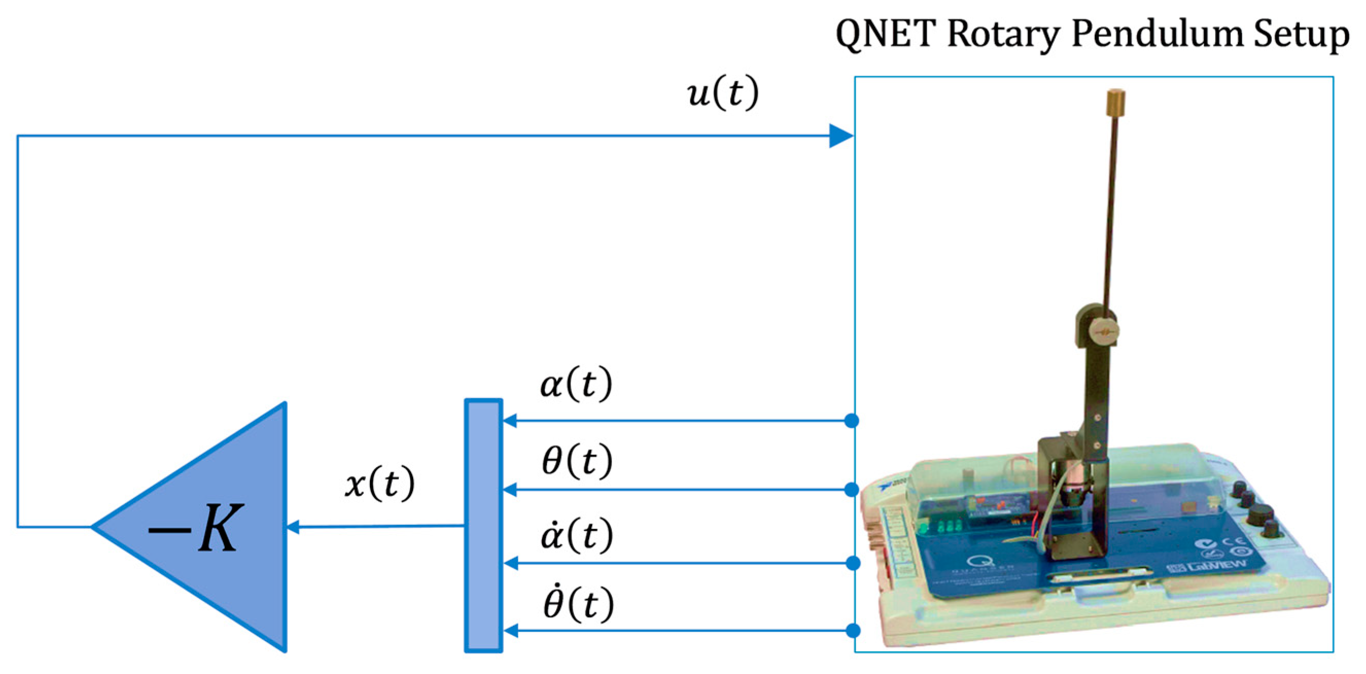
Since Q 0 and R > 0 , it follows that V ˙ t < 0 , ensuring the LQR law maintains asymptotic stability. The block diagram of the LQR law is depicted in Figure 2.

3. Proposed Control Methodology

The prescribed self-regulating FLQR method for the position regulation of the SLRIP systems is systematically formulated in this section.

3.1. Fuzzy-Based Linear Quadratic Regulator (FLQR)

The FLQR strategy is introduced to improve the resilience of the SLRIP system against parametric uncertainties and external disruptions. The proposed control procedure integrates the LQR’s optimal control capabilities with the adaptive nature of fuzzy logic to adaptively reconfigure the control actions as the error dynamics vary [29]. The main goal of this approach is to enhance the system’s transient behavior and strengthen its ability to damp oscillations while preserving its control input economy. The proposed FLQR is realized by designing a customized linear decomposition function (LDF) that decomposes the baseline LQR control law into two components: a CSE variable and a CSED variable. To acquire the said compounded error variables, the state feedback gain vector of the LQR law is rewritten as shown in Equation (20), [29].
K ^ = k α k θ 0 0 0 0 k α ˙ k θ ˙
The formulation of the LDF for the SLRIP is defined as follows [29].
ε t ε ˙ t = K ^ x t
s u c h   t h a t ,     ε t = k α   α t k θ   θ t ,
a n d ,     ε ˙ t = k α ˙   α ˙ t k θ ˙   θ ˙ t .
where ε t is the CSE variable and ε ˙ t is the CSED variable. The arrangement above consolidates the system’s multiple state variables into the CSE and CSED. These aggregated variables encapsulate the system’s dynamic behavior and simplify the implementation of the FIS to generate an adaptive and robust control input. The FIS leverages fuzzy logic principles to enhance the system’s adaptability and robustness by dynamically re-adjusting control actions in response to state variations and disturbances. It employs a set of heuristically designed fuzzy logic (qualitative) rules and predefined membership functions (MFs) to infer precise control actions from input data. The fuzzy logical rules are formulated using the expert’s knowledge to regulate the control effort as a function of the system’s tracking error variations. Considering the operational requirements of the SLRIP’s balancing control problem, the meta rules established to construct the fuzzy qualitative rules are listed below.
  • Amplify the control effort when the system deviates from the desired state.
  • Reduce the control effort as the system approaches the stable equilibrium.
The above rules are computationally implemented for the online refinement of control actions through a two-input Mamdani-type FIS, where the inputs are derived from the error dynamics of the system. The two compounded error variables are normalized (between −1 and +1) by processing them through a cubic HTF [21]. The cubic HTF is employed in this study due to its favorable combination of smooth saturation, odd symmetry, and adjustable steepness via tunable variation rate [21]. Its waveform ensures smooth normalization of the error signals within the bounded range of ±1. Moreover, its cubic formulation introduces selective amplification and suppression regions, such that it significantly attenuates small error fluctuations, reducing unnecessary control effort and chattering, while sharply amplifying larger errors to ensure rapid corrective action [21]. The cubic HTF is preferred over other odd-symmetric functions, like the hard-tanh or soft-sign functions. The hard-tanh function renders abrupt transitions, which introduce discontinuities or chattering in control signals [44]. On the other hand, the soft-sign function offers gentler scaling but weaker nonlinearity near the origin. This cubic nonlinear scaling enhances the controller’s sensitivity in critical conditions, improving control efficiency and robustness [45]. The normalized compounded error variables are expressed below.
ε n t = tanh γ   ε t 3
ε ˙ n t = tanh δ   ε ˙ t 3
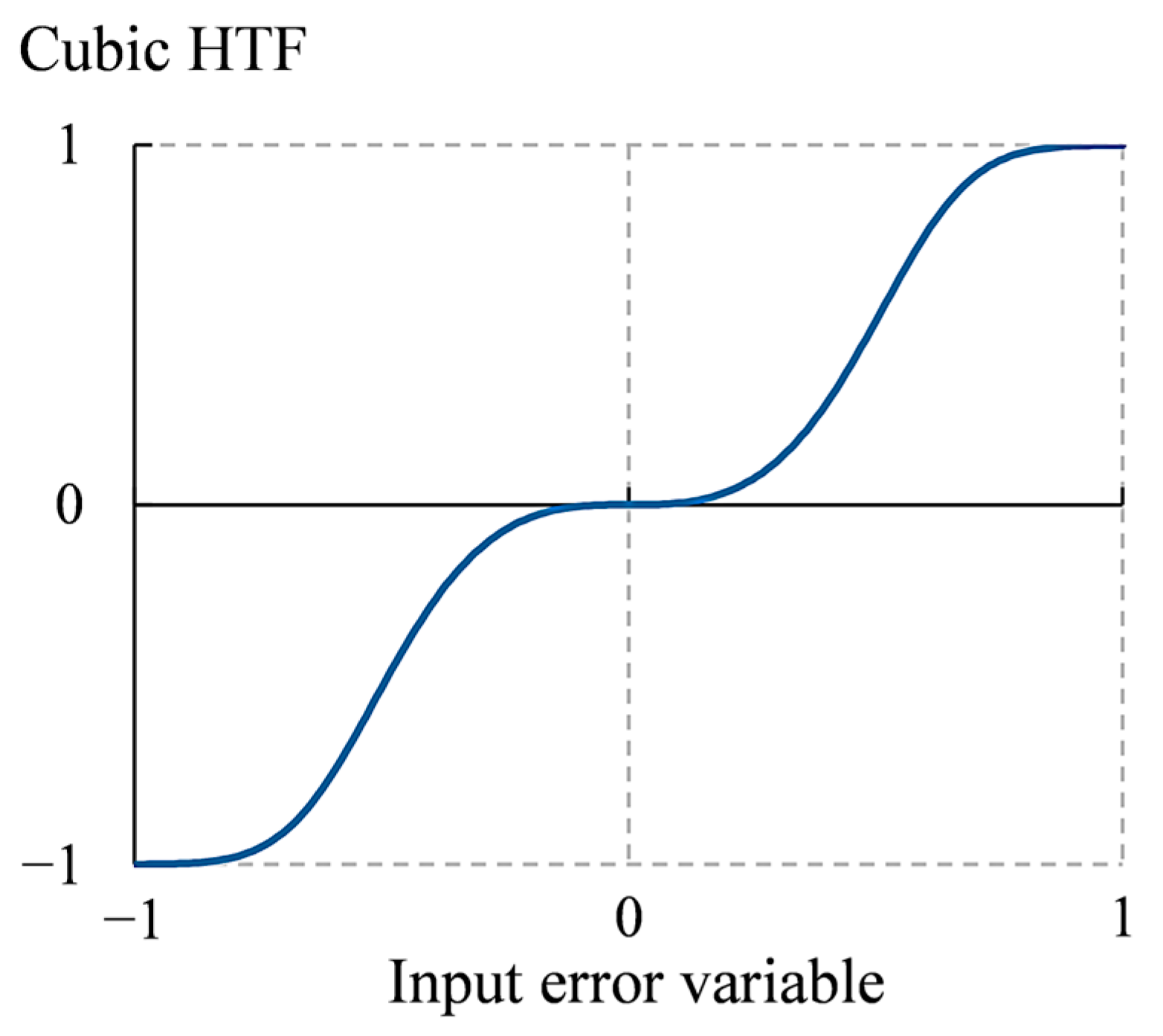
where tanh . represents the HTF, and γ and δ are the pre-determined variation rates of the HTFs. The parameters γ and δ are determined by using the offline tuning procedure (explained in Section 4). The cube of the CSE and CSED is fed the input to the HTFs. The waveform of the prescribed cubic HTF, formulated in Equations (22) and (23), with respect to an input error variable is depicted in Figure 3.
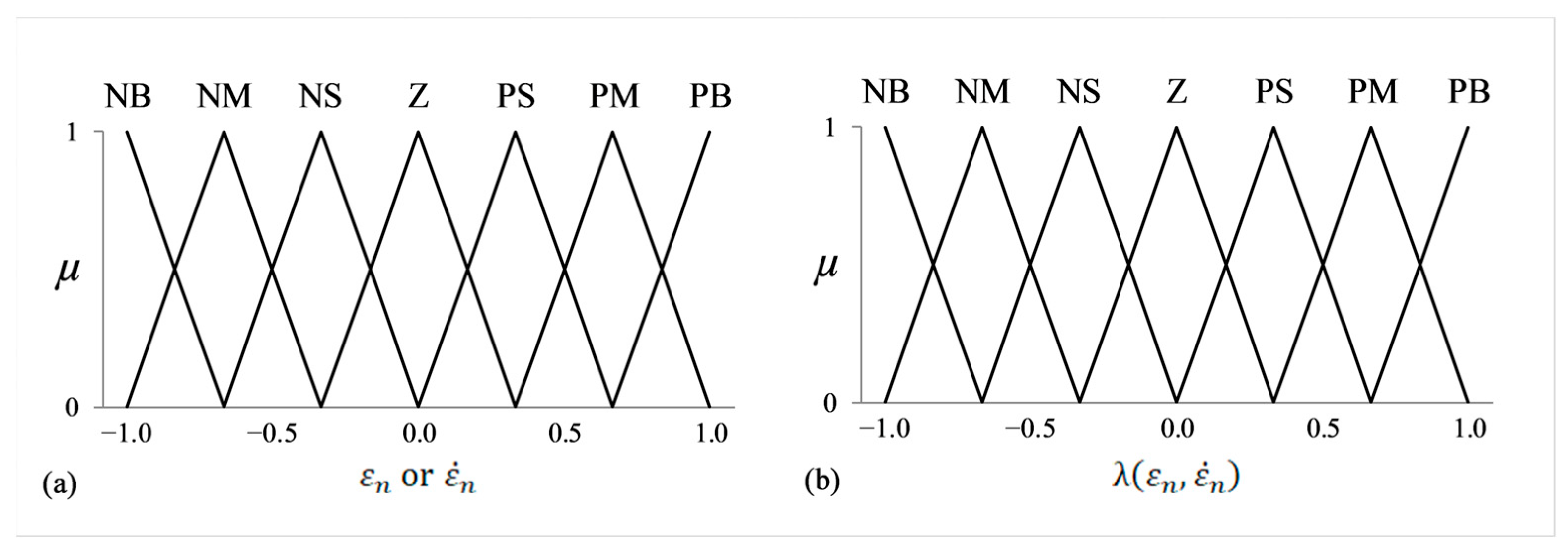
As discussed earlier, the formulation of the cubic HTF generates distinct amplified and suppressed error regions, as illustrated in Figure 3, leading to a sharp increase in the magnitude of ε n t and ε ˙ n t under large error conditions, while significantly reducing it for smaller errors [46]. The preprocessing of CSE and CSED variables via the above-mentioned CHTFs not only normalizes them within ±1 but also creates selective attenuation and amplification regions for improved control efficiency. The normalized error variables ε n t and ε ˙ n t serve as inputs to the FIS, while the normalized control action λ ε n , ε ˙ n serves as the output of the FIS. The crisp input values are converted into fuzzy linguistic variables by the fuzzification module. The input and output variables are classified into seven linguistic categories: Negative Big (NB), Negative Medium (NM), Negative Small (NS), Zero (Z), Positive Small (PS), Positive Medium (PM), and Positive Big (PB). Table 2 presents the complete fuzzy rule-base, which consists of 49 qualitative rules. For fuzzy implication, the max-min inference method stated in Equation (24), is employed.
μ i = min g i ε n , g i ε ˙ n
where μ is the degree of the MF, i is the number of rule, and g i . is the triangular input MF of the following form [16].
g f = 1 + f c i b i ,     b i f c i 0 1 f c i b i + ,     0 f c i b i + 0 ,                 o t h e r w i s e
where f represents the normalized value of the input ε n and ε ˙ n , while b i , c i , and b i + correspond to the left-half width, centroid, and right-half width of the input MF, respectively. Symmetrical triangular MFs are adopted in this work to simplify computation during fuzzy implication and aggregation.
The waveforms of the input MFs as well as the output fuzzy MFs are depicted in Figure 4a and Figure 4b, respectively. While the membership functions appear visually similar due to the use of identical triangular shapes and evenly spaced centroids for design uniformity, Figure 4a corresponds to the fuzzification of the compounded error variables, whereas Figure 4b represents the output control signal space. The centroid defuzzification method, defined in Equation (26), is used to acquire the crisp output λ ε n , ε ˙ n [16].
λ ε n , ε ˙ n = i = 1 N μ i   w i i = 1 N μ i j
where w represents the output MF’s centroid, and N = 49 denotes the number of fuzzy rules. The resulting crisp output is then processed using the saturation function, formulated in Equation (27), to generate the refined control action.
u t = V s a t tanh λ ε n , ε ˙ n
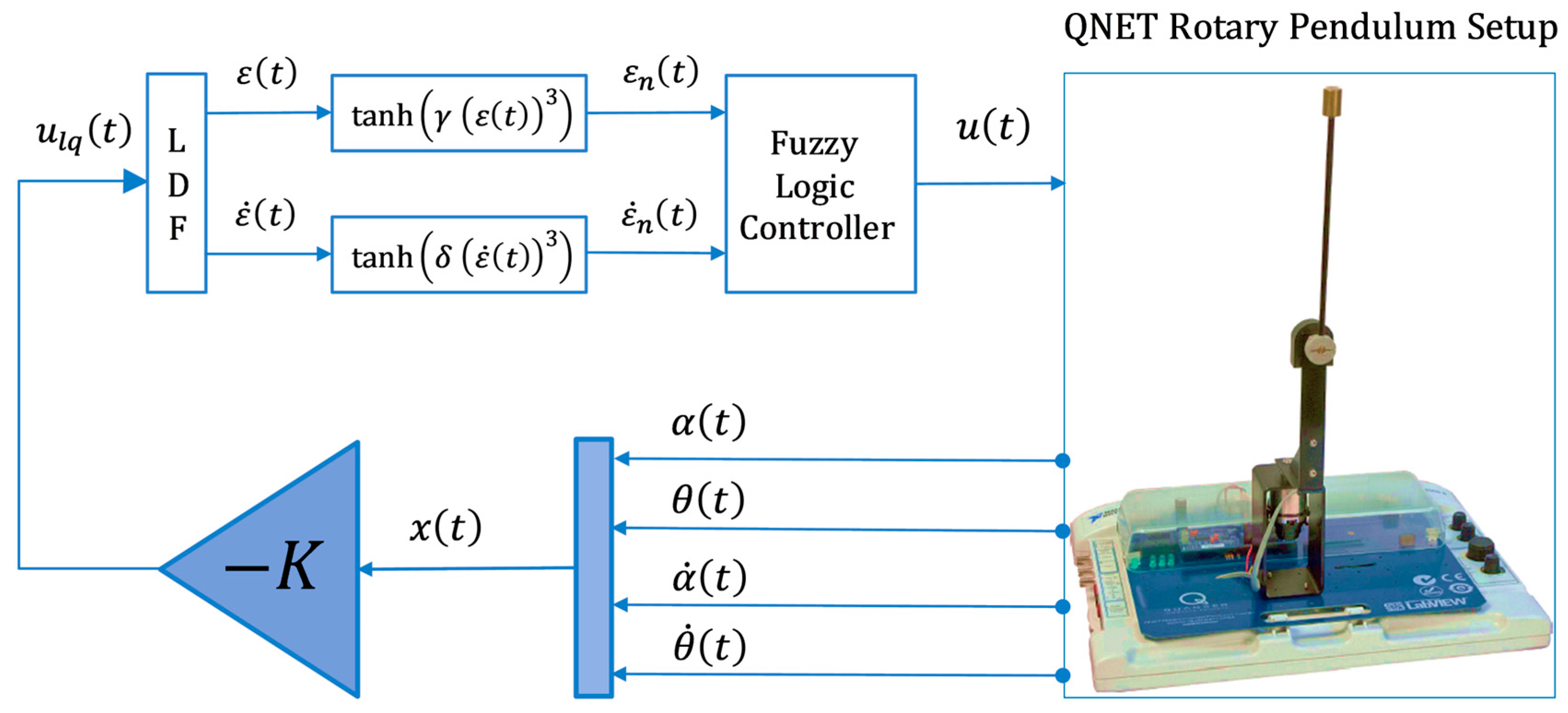
where V s a t sets the lower and upper bounds of the applied control input, preventing the SLRIP’s actuator (DC motor) from getting saturated. The value of V s a t is set to 15.0   V as per the guidelines provided in [32]. The schematic of the FLQR scheme is shown in Figure 5.

3.2. Self-Regulating FLQR Law

The selection of fixed variation rates for the CHTFs, in the FLQR law, formulated for the nonlinear preprocessing of the CSE and CSED variables, presents a fundamental limitation, as it constrains the controller’s adaptability to reject parametric variations and environmental uncertainties. This issue is addressed by dynamically self-regulating the variation rates through a model-free online adaptive tuning law, which optimizes the inflation or depreciation of the applied control force in real time. This enhancement improves system sensitivity and responsiveness, allowing the controller to efficiently modulate control effort, minimize oscillations, and compensate for disturbances with reduced energy consumption.
The online self-tuning mechanism, proposed in [47], is employed due to its robust tracking performance. It is formulated by using pre-configured anti-dissipative and dissipative functions that adjust the hyperbolic function’s variation rates after each sampling interval based on the system’s CSE and CSED variables [39,45]. The formulations of the aforesaid Variance Adaptation Functions (VAFs) are expressed as follows [47].
γ ˙ t = σ 1 γ t + β 1 ε t 2  
δ ˙ t = σ 2 δ t + β 2 ε t ε ˙ t
where σ 1 and σ 2 represent the pre-configured positive decay rates, and β 1 and β 2 represent the pre-configured positive adaptation rates associated with the online adaptation functions. The parameters governing adaptation and damping rates are optimized as per the offline tuning method described in Section 4. The constructed VAFs dynamically regulate the stiffness or softness of control action depending on the state’s deviations from the reference, ensuring adaptive performance. Each of these VAFs consists of a dissipative term and an anti-dissipative term, as demonstrated below.
Dissipative term: σ 1 γ t σ 2 δ t Anti-dissipative term: β 1 ε t 2 β 2 ε t ε ˙ t
Each of these terms serves a specific purpose while modifying the variation rate. The rationale is presented as follows [47].
  • Dissipative term: Reduces the variation rate under small error conditions, ensuring gentle settlement of the response as it approaches reference, reducing steady-state fluctuations, and preventing wind-up.
  • Anti-dissipative term: Amplifies the variation rate when the state error increases, promoting an aggressive control action to suppress overshoots, while speeding up the transient recovery response.
The VAFs formulated in Equations (28) and (29) are unified as a first-order differential equation, expressed in Equation (30).
v ˙ t = H v t + M ϵ t
s u c h   t h a t ,   v t = γ t δ t , H = σ 1 0 0 σ 2 , M = β 1 0 0 β 2 , ϵ t = ε t 2 ε t ε ˙ t
where v t represents a vector of time-varying variation rate gains, while ϵ t denotes a vector containing state-error-dependent terms. The H and M matrices are positive-definite, where H contains the decay rates σ 1 and σ 2 , and M includes the adaptation rates β 1 and β 2 . At each sampling interval, the ordinary differential equation in Equation (30) is integrated numerically to determine v t , thereby updating the variation-rates. The variation rate adaptation process is computationally realized by solving the ordinary differential equation in Equation (30), as expressed in Equation (31).
v t = e x p H t v 0 + 0 t e x p H t p M ϵ p d p
where exp . denotes the exponential function. The initial variation rate vector v 0 contains the offline optimized values of γ and δ (refer to Section 4). The coefficients of the vector v t are adaptively modified online after each sampling interval based on the system’s state and error variations. The rate adaptation process initiates with the initial variation rates, v 0 , prescribed for FLQR in Section 4. As long as the exponent of the exponential term H remains negative definite, e x p H t decays to zero over time. This behavior ensures that the proposed adaptation law exhibits exponential stability, as the output progressively diminishes. These VAFs deliver time-varying variation rates γ t and δ t , which are then incorporated into the cubic HTFs. The expressions of the self-regulating CSE and CSED variables are shown in Equations (32) and (33).
ε n , s r t = tanh γ t   ε t 3
ε ˙ n ,   s r t = tanh δ t   ε ˙ t 3
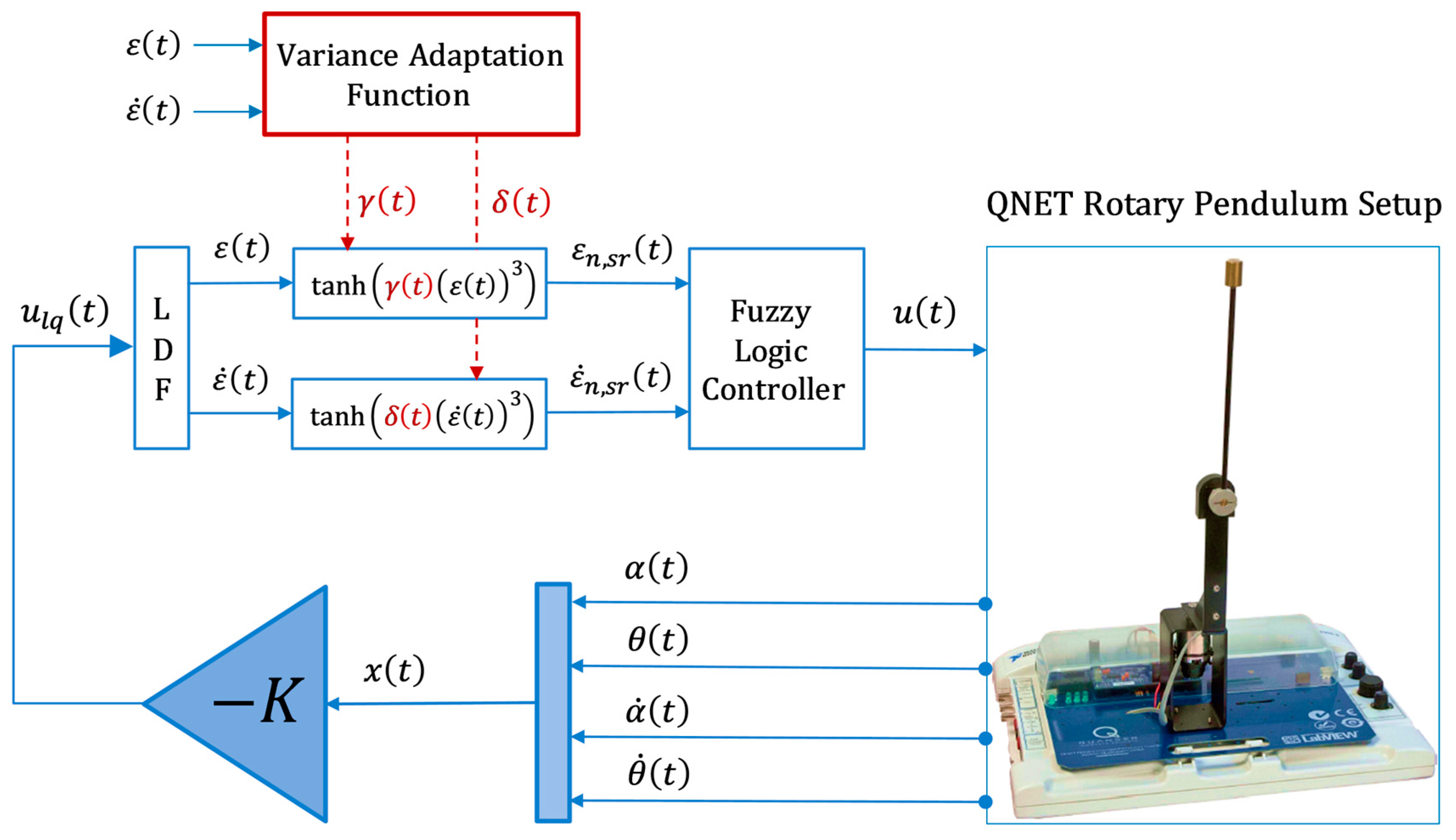
where ε n , s r t and ε ˙ n ,   s r t represent the self-regulating compounded error variables. After adaptive preprocessing via VAFs, the modified compounded error variables are fed directly to the FIS as input variables for the computation of the final control action. This arrangement dynamically reconfigures the shape and form of the cubic HTFs as per the state deviations, influencing the normalized CSE and CSED variables to manipulate the strength of the damping control action yielded by the FIS. Thus, apart from normalizing the input variables within ±1 for improved fuzzy reasoning and introducing selective attenuation and amplification regions to enhance control input efficiency, the designed VAFs adaptively reconfigure the waveform of CHTF to improve the FLQR’s flexibility and responsivity to effectively reject external disturbances. Consequently, the system efficiently mitigates overshoots, steady-state fluctuations, and disruptive control actions. The proposed control procedure is referred to as the Self-Regulating FLQR (SR-FLQR) law. The block diagram of SR-FLQR law is illustrated in Figure 6.

4. Parameter Optimization Method

The effectiveness of the LQR depends on both the system’s state deviations and the adjustments in the control signal. The optimal control performance is achieved by appropriately selecting the weighting factors for the state matrix Q = d i a g q α q θ q α ˙ q θ ˙ and control input factor R = ρ . The operation of the FLQR scheme is dictated by the optimal selection of the pre-determined variation rates, γ and δ , of the HTFs. Similarly, the performance of the proposed self-regulating FLQR scheme, formulated in Section 3.2, is influenced by the predefined selection of the learning gains ( σ 1 , σ 2 , β 1 , and β 2 ) associated with the VAFs that dynamically reconfigure the waveform of the HTFs.

4.1. Tuning Algorithm

To optimize the aforementioned controller parameters offline, the cost function in Equation (34) is minimized [21].
J c = 0 T e α t 2 + e θ t 2 + u t 2 d t
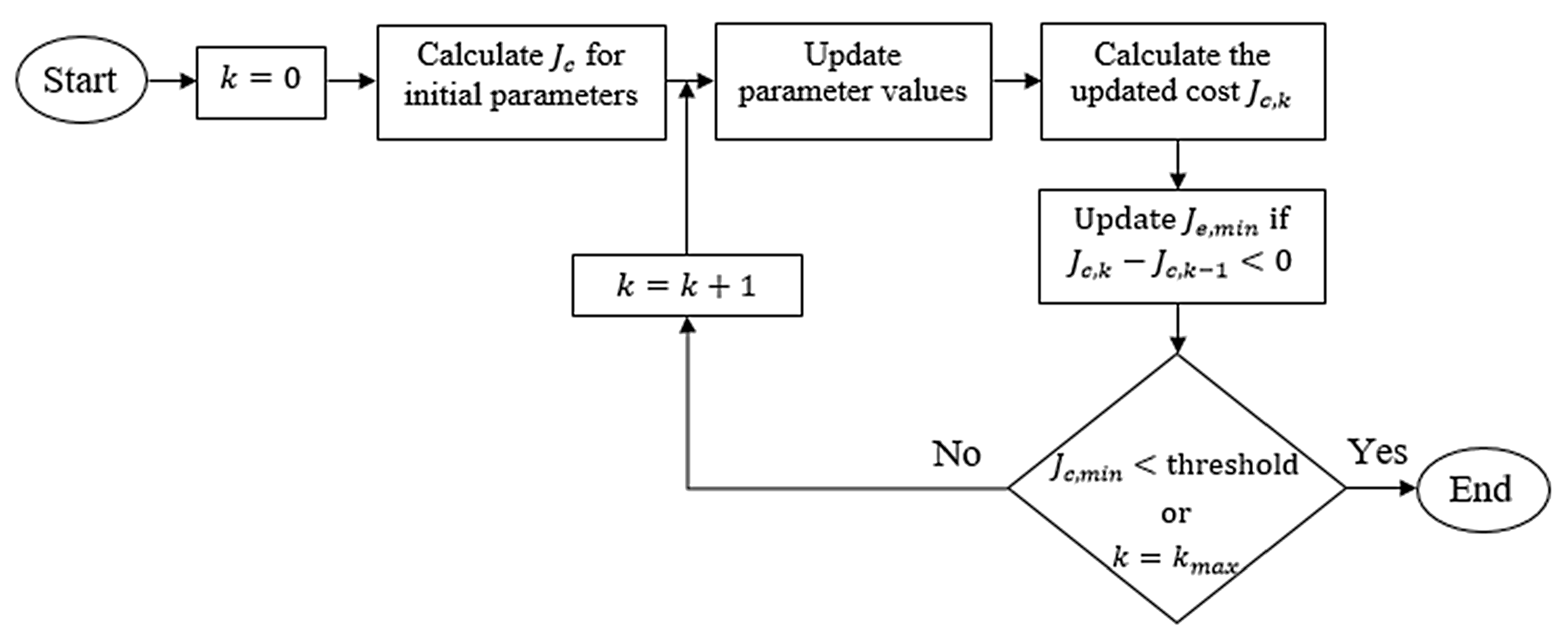
where T represents the duration of an experimental trial, e α t = α t α 0 and e θ t = θ t π , denote the deviation (or error) in the horizontal arm and pendulum link from their respective reference positions. The pendulum link’s reference position is set at π radians, while the arm’s reference is set at its initial position, α 0 . Equal weights are applied to the variables in the cost function J c to ensure a balanced compromise between tracking accuracy and control efficiency. This approach avoids biasing the controller toward any single objective. This setting ensures that neither the position errors nor the control effort are overly prioritized, leading to a well-rounded controller that maintains accurate reference tracking while minimizing excessive control actions. For the baseline LQR design, the weighting coefficients for the state error and control cost terms are selected within the range [0, 100] to balance performance and energy efficiency [1]. For the FLQR design, the variation rates, γ and δ , of the HTFs are selected within the range [0, 10]. For the self-regulating FLQR design, the decay rates ( σ 1 and σ 2 ) and adaptation rates ( β 1 and β 2 ) associated with the VAFs are selected within the range [0, 1] and [0, 10], respectively. The parameter selection and tuning process is depicted in Figure 7 [21]. The experimental implementation details are provided in Section 5.
The tuning procedure begins by setting all initial controller parameters to unity. Each iteration involves modifying the designated control parameters, manually positioning the pendulum rod in an upright state, and balancing it for a duration of 10 s to evaluate the corresponding cost J c , k , where k denotes the trial number. The optimization follows a gradient-based approach, iteratively refining the parameters to minimize the cost function [21]. If the cost associated with the current trial, J c , k , is less than that of the preceding trial, J c , k 1 , the local minimum cost, J c , m i n , is revised accordingly.
The tuning process terminates when either the predefined maximum number of trials, k m a x , is reached or J c , m i n falls below a specified threshold. The termination threshold is empirically determined through preliminary algorithmic trials, which assess different threshold values to achieve the best trade-off between solution accuracy and computational efficiency while avoiding premature convergence. In this study, the initial minimum cost is recorded as J c , m i n 0 0.89 × 10 6 [21]. A scaling factor of 0.01 is applied to establish the stopping criterion, ensuring efficient convergence while mitigating unnecessary computational complexity. A larger scaling factor would impose an excessive computational cost, whereas a smaller factor risks premature termination. Consequently, the algorithm concludes when J c , m i n reaches 0.01   J c , m i n 0 . For this study, the final threshold values for J c , m i n and k m a x are set at 1 × 10 4 and 30, respectively.

4.2. Controller Parameterization

Upon completion of the optimization process, the following set of parameters is acquired. For the LQR, the weighting coefficients of the state and control matrices are obtained as Q = d i a g 32.82 52.23 6.12 2.51 and R = 1.02 . The corresponding state feedback gain matrix, computed using (15), is K = 6.21 130.56 4.22 17.83 . For the FLQR design, the variation rates of the cubic HTF used to normalize the compounded error and its derivative are obtained as γ = 1.59 and δ = 0.87 . For the SR-FLQR design, the learning gains associated with the VAFs are selected as σ 1 = 0.082 , σ 2 = 0.065 , β 1 = 3.14 , and β 2 = 2.61 .

5. Experimental Results and Discussions

This section details the hardware-in-loop (HIL) implementation of the designed control procedures on Quanser’s SLRIP platform.

5.1. HIL Implementation

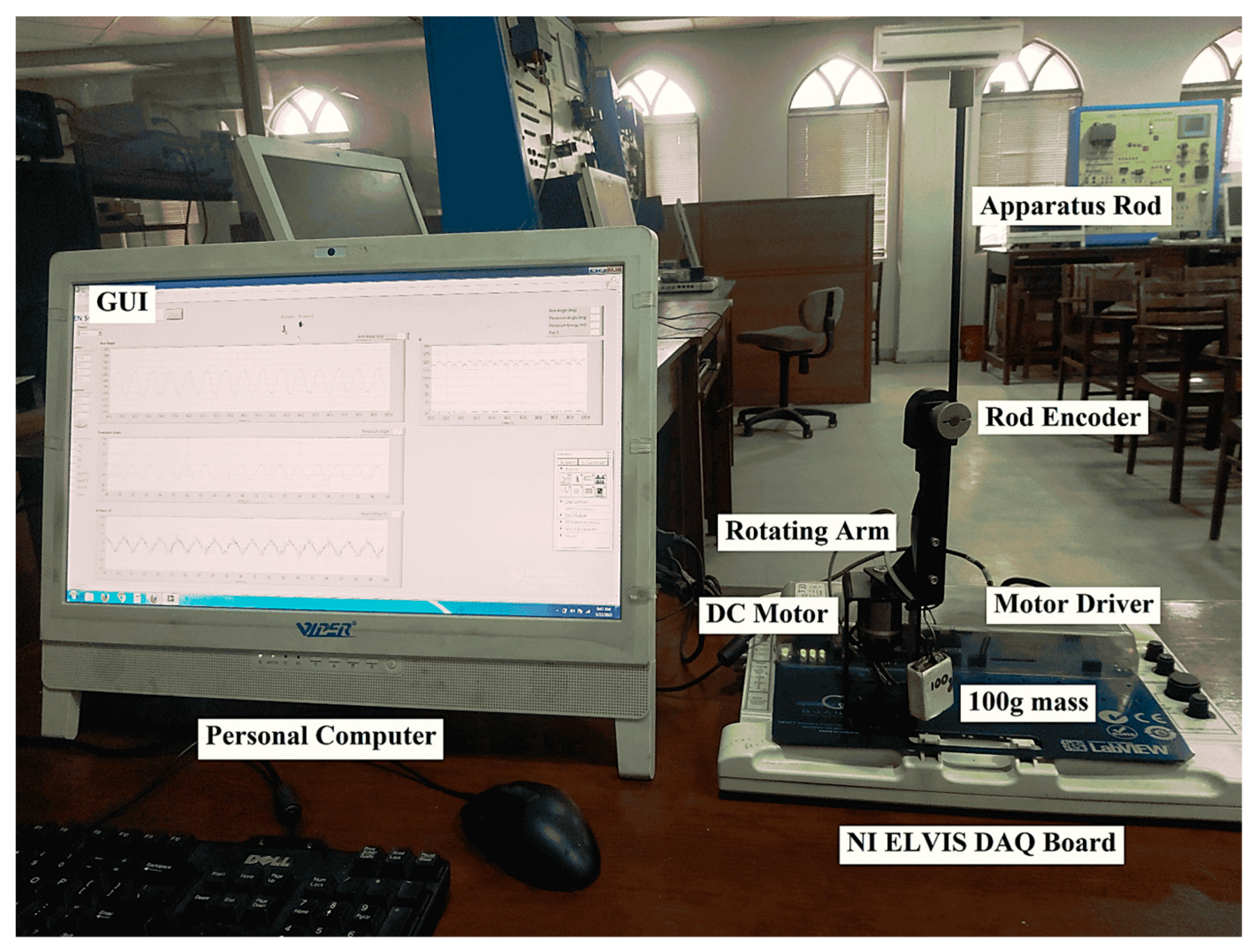
The resilience of the designed control procedures is evaluated through customized experiments conducted on the Quanser rotary pendulum platform, depicted in Figure 8.
The angular positions of the SLRIP’s arm and rod are measured using high-resolution encoders at a 1.0 kHz sampling frequency, with data acquisition performed via an NI-DAQ Board. The encoder resolution was explicitly accounted for in the digital implementation. The measured angles are obtained from raw encoder counts as shown in Equation (35).
θ = 2 π N C
where N is the encoder counts and C is the encoder resolution in counts per revolution. This conversion ensures that the control algorithm operates on precise angular states rather than raw counts, thereby maintaining accuracy in the feedback loop. The received signals are filtered and then communicated to the control application over a 9600-bps serial link. A customized LabVIEW-based software application is developed using LabVIEW 2018’s Block Diagram tool. The control software runs on a 64-bit, 2.1 GHz Intel Core i7 processor with 16 GB RAM, which efficiently handles the fuzzy logic computations as well as the recursive computations associated with the online variance adaptation functions. These functions are implemented using C-language programming within LabVIEW’s Math Script tool, while additional required functions are selected from the function palette. The customized graphical user interface of the control application provides real-time monitoring and data logging of the system’s control input and state variations. The angular velocities of both the pendulum link and the rotary arm were computed from encoder position measurements by numerical differentiation, followed by low-pass filtering to suppress measurement noise. These filtered velocity estimates were then used in the control computations. The control algorithm continuously performs the fuzzy logic computations and updates the control signal at each sampling interval, leveraging the real-time clock of the embedded processor. The SLRIP’s onboard motor driver modulates these updated signals to actuate the DC servomotor, ensuring safe operation under discontinuous control demands. Each experiment begins with the manual stabilization of the pendulum link, ensuring consistent initial conditions for a fair performance comparison.

5.2. Experimental Validation

To assess the performance and robustness against disturbances, each prescribed control procedure is tested to maintain the pendulum link in the upright position and the horizontal arm at its initial (reference) position. The following HIL experiments are used to validate system resilience.
A.
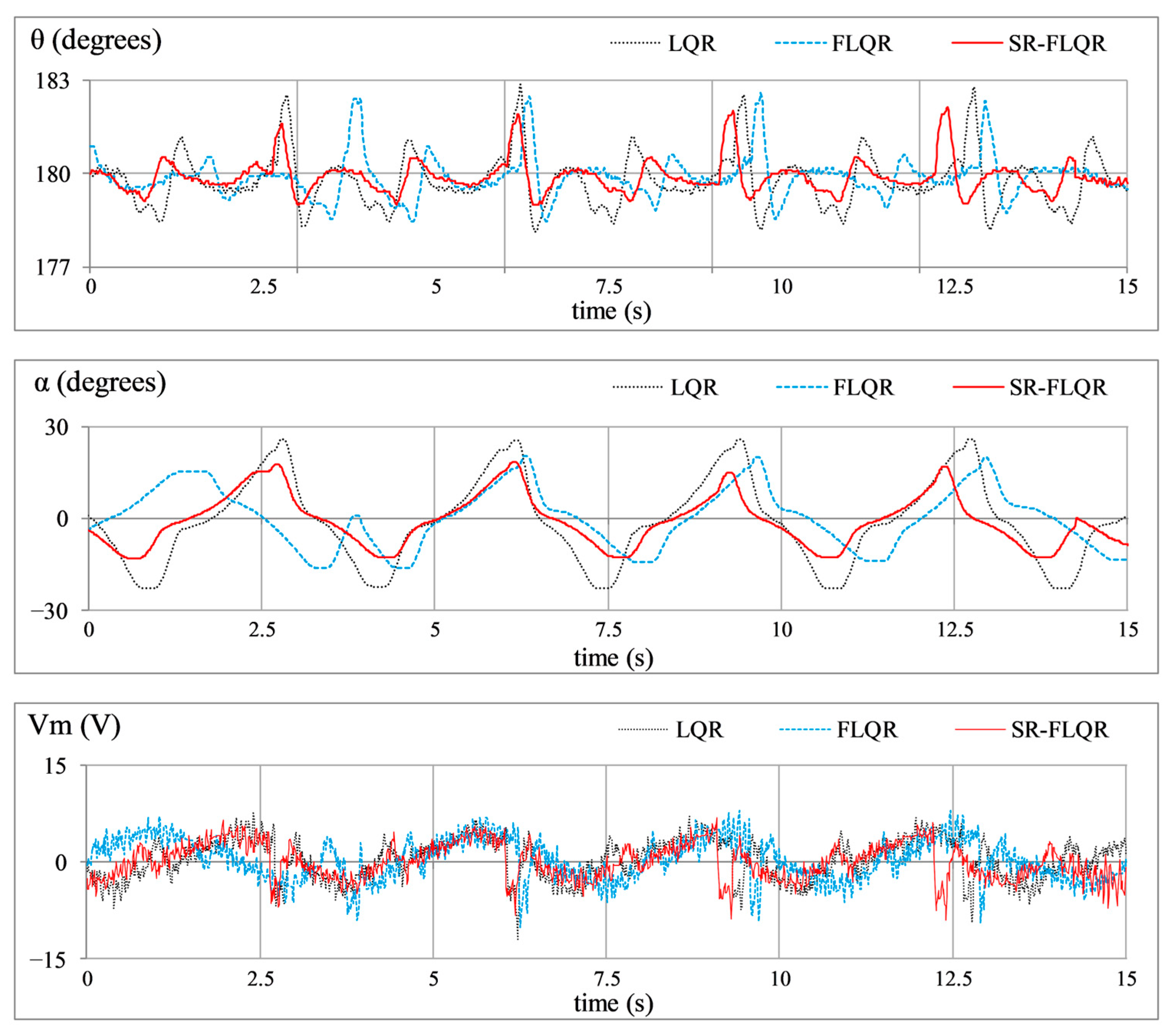
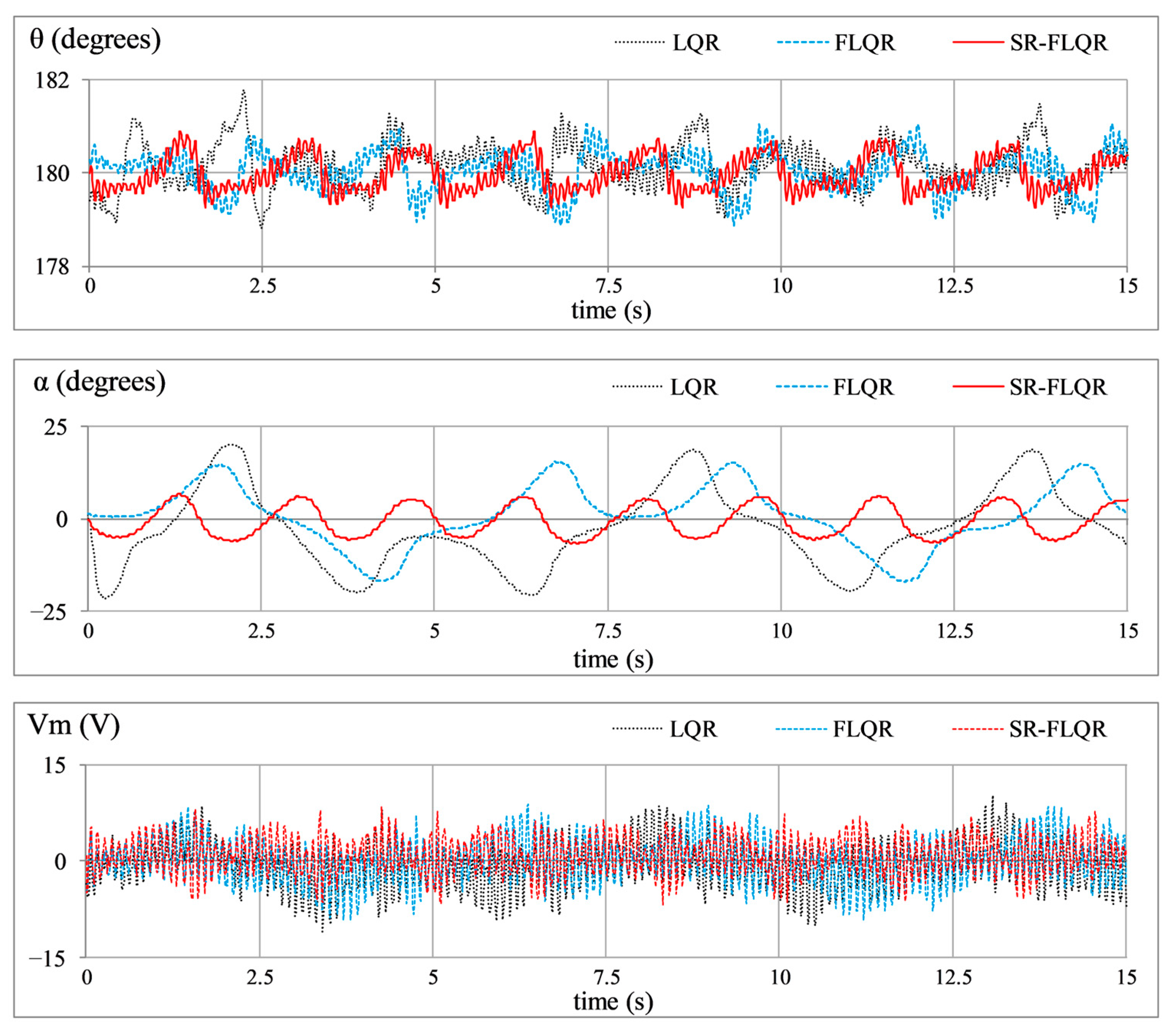
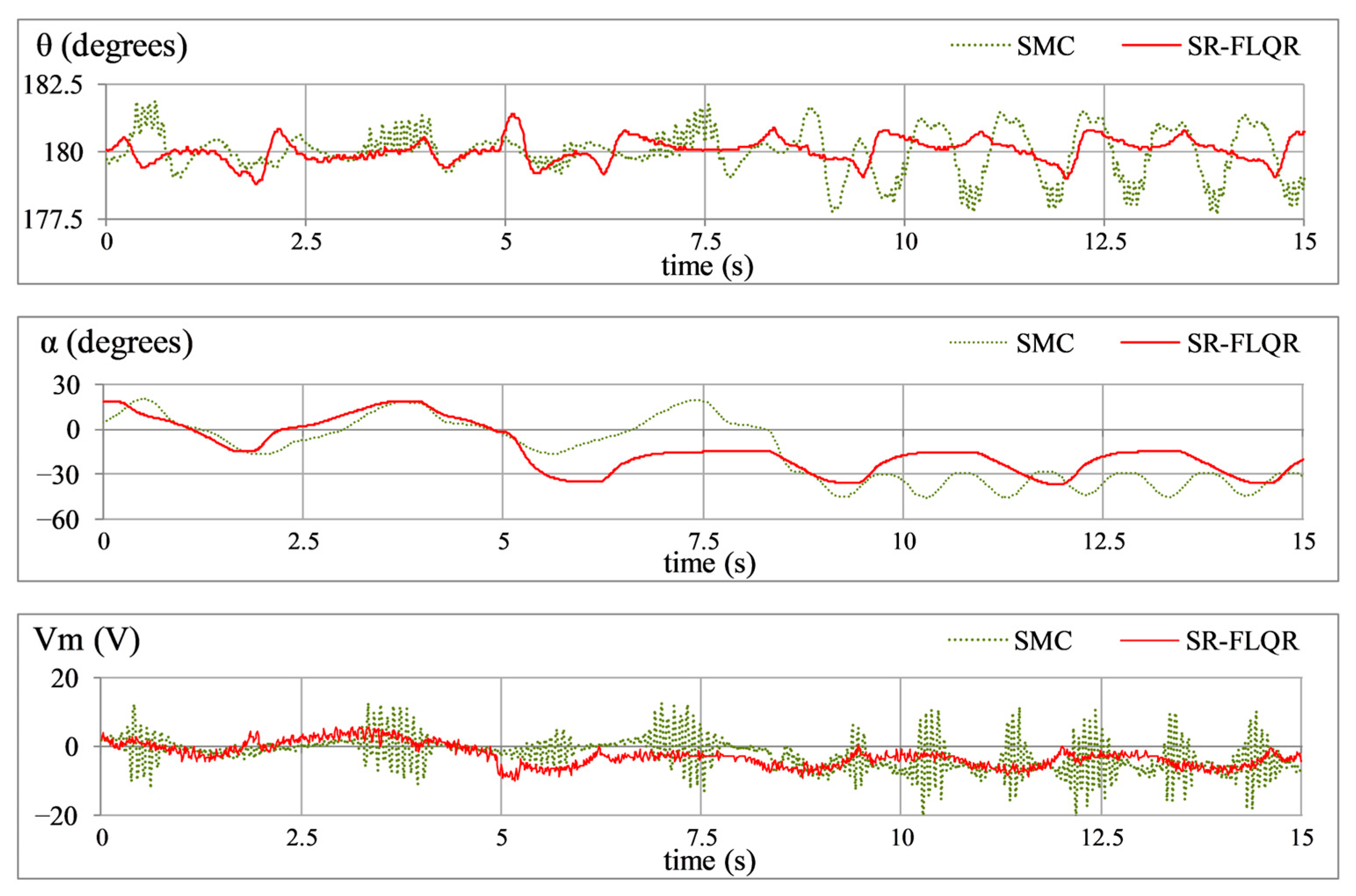
Position Regulation: This baseline experiment evaluates the system’s ability to maintain its reference positions without external disturbances. It replicates real-world scenarios where a robotic system or an industrial manipulator must remain stable under normal operating conditions. The time-domain profiles of θ t , α t , and V m t are manifested in Figure 9.
B.
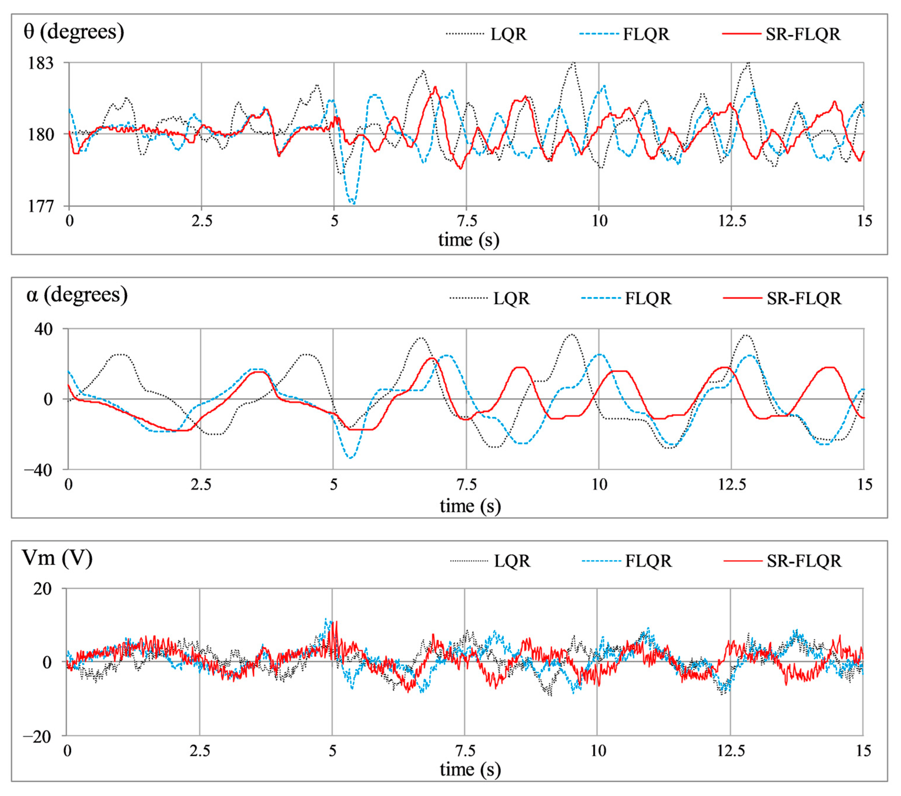
Impulse Disturbance Rejection: This experiment is conducted to evaluate the system’s response to transient impacts. An impulse disturbance is injected into the control input to assess the system’s capability to recover from sudden external shocks, such as power transients, abrupt mechanical impacts, sudden hardware failures, or seismic forces in engineering applications. A simulated 5.0 V pulse, having a span of 100 ms, is applied whenever the horizontal arm reaches its maximum position. The corresponding profiles of θ t , α t , and V m t are illustrated in Figure 10.
C.
Step Disturbance Compensation: This experiment evaluates the effect of a sudden and sustained external force, similar to wind gusts on aircraft, ocean currents affecting marine vessels, or sustained mechanical loads on industrial robots. A −5.0 V step input is introduced in the control signal at t = 10 s to examine the control scheme’s ability to manage abrupt but constant disturbances. The resulting variations in θ t , α t , and V m t are depicted in Figure 11.
D.
Sinusoidal Disturbance Attenuation: This test examines the control system’s resilience against periodic disturbances and mechanical vibrational effects, which are very common in robotics, aerospace, and automotive control systems. Although real disturbances such as sensor noise, friction, and backlash are non-periodic in nature, a sinusoidal disturbance is employed for this test case as a structured input to systematically test the controller’s robustness. The sinusoidal disturbance provides a repeatable and well-defined disturbance with continuous excitation across time, which makes it suitable for stressing both the tracking and regulation capabilities of the controller [48]. Moreover, stochastic disturbances are inherently present during the hardware experiments, meaning the proposed controller was simultaneously exposed to realistic non-periodic perturbations as well. A sinusoidal disturbance signal of the form, d t = sin 20 π t , is injected into the control signal to evaluate robustness. The corresponding responses of θ t , α t , and V m t are shown in Figure 12.
E.
Model Error Rejection: This scenario assesses the controller’s capacity to compensate for model inaccuracies and parametric variations, which occur in real-world applications where the system dynamics evolve/alter over time. To simulate this effect, a 0.1 kg mass is attached beneath the pendulum link, creating a mismatch between the real and modeled system dynamics. The system’s adaptability to this perturbation is investigated via the time domain profiles of θ t , α t , and V m t shown in Figure 13.

5.3. Analysis and Discussions

The following seven Quantitative Performance Measures (QPMs) are used to evaluate each controller’s performance under the given test scenarios.
  • RMSEz—Root mean square (RMS) error in the pendulum link and arm positions.
  • Mp,θ—Peak overshoot magnitude of the rod following a disturbance.
  • Ts,θ—Time required for the pendulum link to settle within ±5% of π rad. reference of the pendulum (~0.157 rad.) after a transient disturbance.
  • αoff—Offset in the horizontal arm’s position after disturbance application.
  • αp-p—Peak-to-peak magnitude of oscillations in the arm after disturbance application.
  • MSVm—Mean squared value of the motor control voltage.
  • Vp—Maximum control voltage after disturbance application.
The RMS error is evaluated as shown in Equation (36).
R M S E z = 1 M k = 1 M e z t 2
where z = α or θ , and M is the number of samples. The settling time Ts,θ is evaluated from the pendulum’s response as expressed in Equation (37).
T s , θ = m i n t   |   e z t 0.157
The mean-squared value of motor control voltage is evaluated as shown in (38).
M S V m = 1 M k = 1 M u t 2
The HIL experimental results confirm that the proposed SR-FLQR scheme exhibits superior position regulation, robust disturbance compensation, rapid response speed, and minimal control energy consumption. A quantitative analysis of the experimental results is presented in Table 3, with a qualitative discussion presented below.
In Experiment A, the fixed-gain LQR exhibits the weakest performance among the tested controllers, exhibiting the highest position-regulation errors and excessive control energy usage. The FLQR improves accuracy and reduces control costs, while the SR-FLQR further enhances tracking precision and energy efficiency. In Experiment B, LQR demonstrates weak disturbance rejection, leading to slow recovery, large overshoots, and high control demands. FLQR mitigates overshoots and speeds up response, but at the cost of disrupted control activity. SR-FLQR ensures faster recovery, better damping, and lower peak control input demands, optimizing efficiency. In Experiment C, LQR fails to compensate for step disturbances, resulting in large angular offsets. FLQR reduces fluctuations, but with erratic control energy usage. SR-FLQR provides faster recovery, better disturbance rejection, and smoother control with lower peak torque requirements. In Experiment D, LQR struggles with sinusoidal disturbances, causing large state fluctuations and poor control efficiency. The FLQR offers better immunity, but SR-FLQR outperforms both by minimizing fluctuations and reducing chattering while maintaining smooth control. In Experiment E, LQR inadequately handles modeling errors, leading to large perturbations. The FLQR improves position regulation and control efficiency, while SR-FLQR delivers the best error compensation with strong damping and optimal energy usage.
Quantitatively, SR-FLQR improves position regulation, energy efficiency, transient recovery, and overshoot reduction by significant margins over both LQR and FLQR. As compared to the baseline LQR, SR-FLQR exhibits a 22.4% improvement in RMSEθ, a 26.2% reduction in RMSEα, and a 22.0% reduction in MSVm under nominal conditions. In the disturbed state, as compared to LQR, the SR-FLQR demonstrates a 25.1% reduction in Mp,θ, a 33.3% reduction in Ts,θ, a 24.7% reduction in the peak servo control demands, a 39.7% improvement in αoff, and a 30.6% enhancement in αp-p. As compared to the baseline FLQR, SR-FLQR exhibits an 11.6% improvement in RMSEθ, a 19.2% improvement in RMSEα, and a 17.2% improvement in MSVm under nominal conditions. In the disturbed state, as compared to FLQR, the SR-FLQR demonstrates a 16.7% reduction in Mp,θ, a 14.8% reduction in Ts,θ, a 10.5% reduction in the peak servo control demands, a 15.1% improvement in αoff, and a 36.9% enhancement in αp-p.
These enhancements stem from its self-regulating weight-adjusting function, which increases adaptability and enables dynamic restructuring of the control scheme for optimal performance. The superior responsiveness of SR-FLQR is evident in its rapid yet precise variance adjustments, allowing it to effectively counteract disturbances.
In practical digital implementations, the proposed SR-FLQR offers strengths such as online self-tuning without requiring explicit system models, robustness against parameter variations, and ease of integration with existing LQR frameworks. However, its limitations include increased computational demand due to the fuzzy inference and variance adaptation layers, potential sensitivity to discretization delays at low sampling rates, and the need for careful tuning of adaptation gains to avoid excessive actuator effort. These aspects should be considered when deploying the controller in embedded hardware with limited resources.

5.4. Comparison with a Robust SMC Controller

To benchmark the proposed control strategy further, a comparison was performed against Gao’s power-rate SMC law, a well-known robust method designed to handle model uncertainties and external disturbances. The SMC was implemented using the same system model and experimental setup. The SMC formulation adopted for comparison in this study follows the control law design proposed in [7], and is expressed in Equation (39).
u t = F T B 1 F T A x t + m s t γ s g n s t
where s t is the sliding surface, F T is a state-error weighting vector, m is a positive scaling factor, γ is the positive fractional power of s t , and s g n . is the “signum” function. The sliding surface s t is computed as shown in Equation (40).
s t = F T p t
s u c h   t h a t ,   p t = x t x r e f
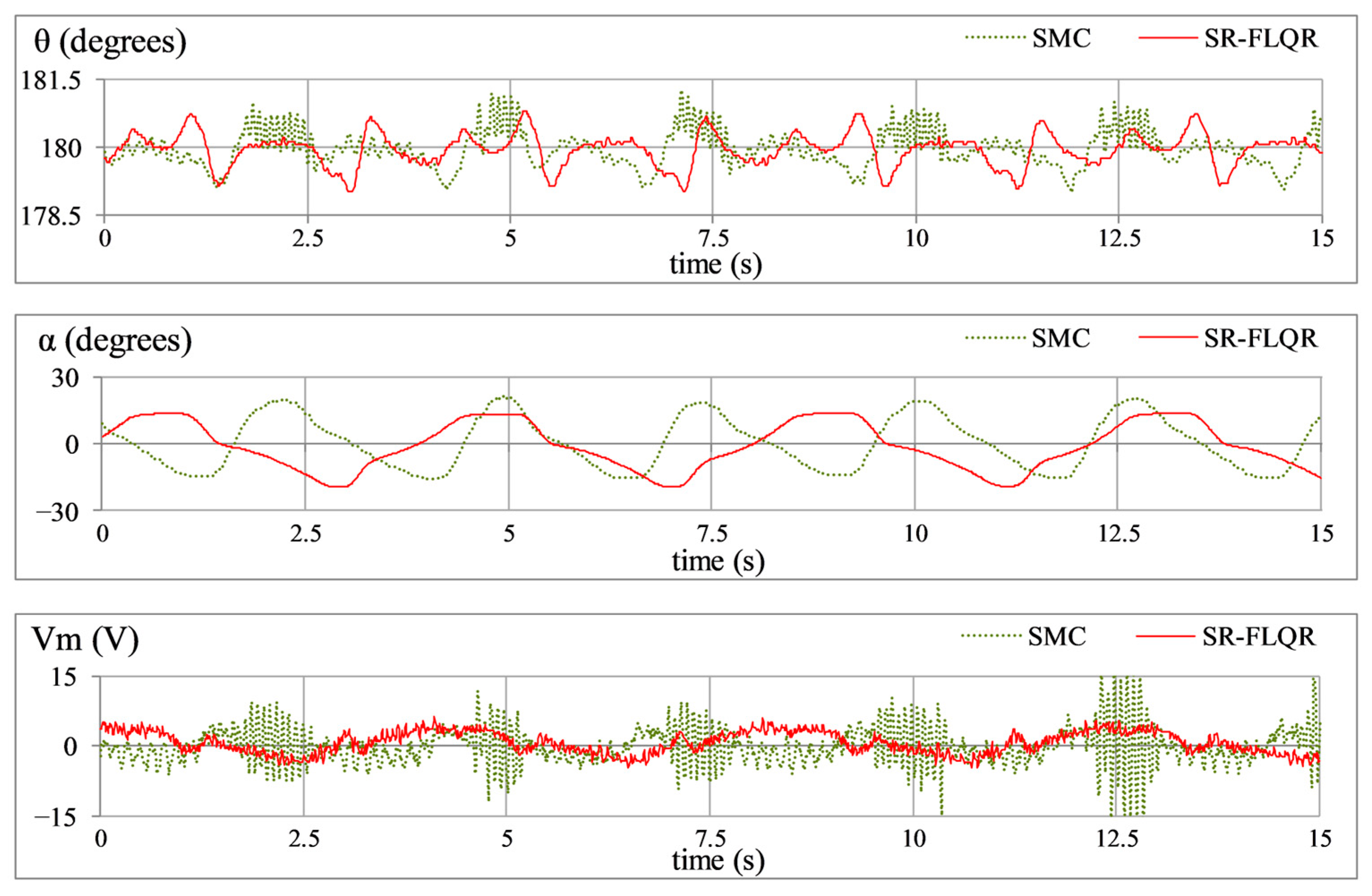
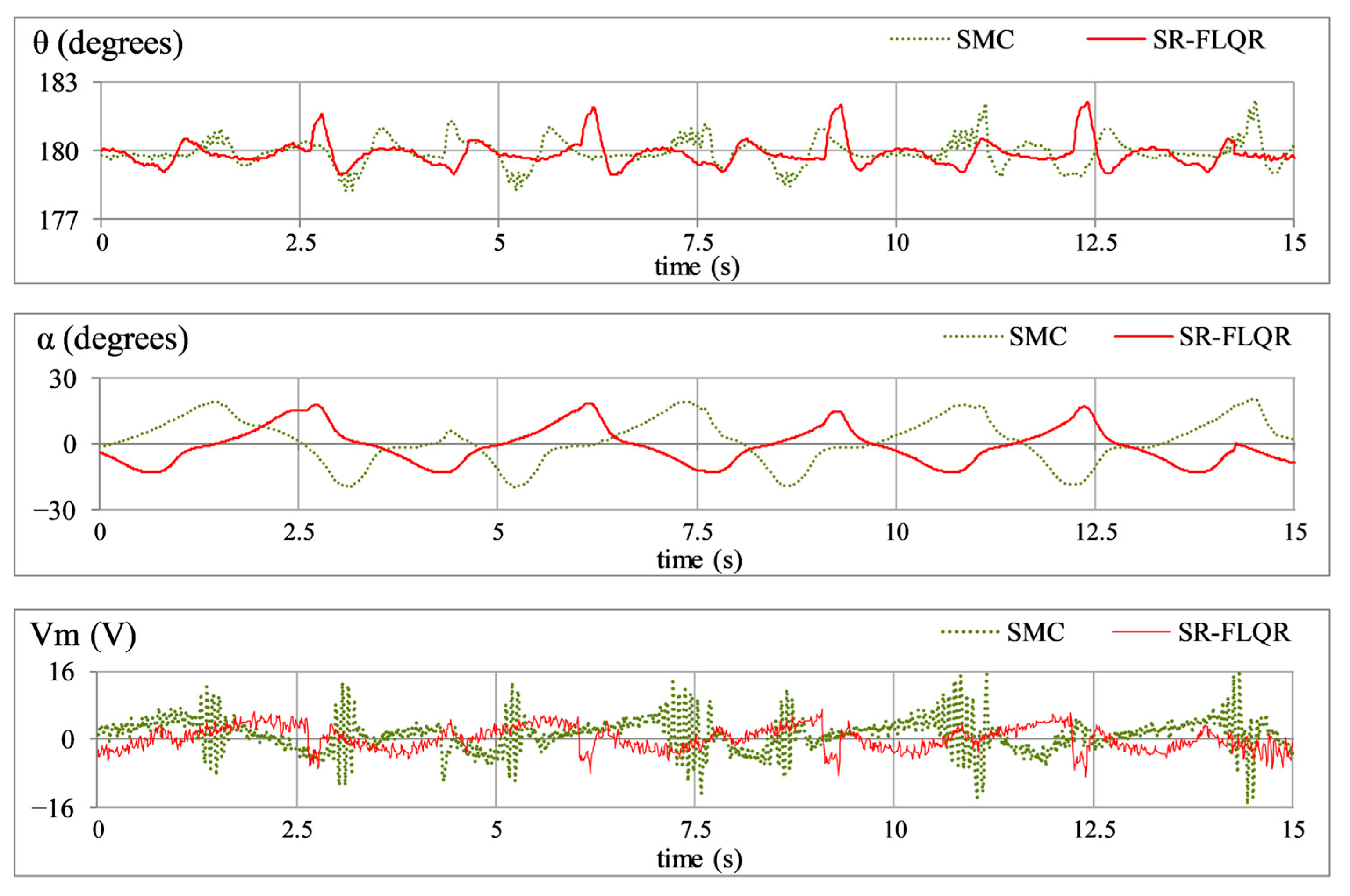
where x r e f = 0 π 0 0 T is the reference state vector. The tuned parameter values used for controlling the Quanser SLRIP system were adopted from the study in [7], with m = 4.07 , γ = 0.45 , and F T = 3.16 73.48 3.02 9.25 . The SMC-regulated SLRIP system is subjected to the same tests as discussed in Section 5.2. The graphical results yielded by Experiments A to E, conducted to compare the performance of the SR-FLQR against the SMC, are shown in Figure 14, Figure 15, Figure 16, Figure 17 and Figure 18.
The experimental results are quantitatively presented in Table 4. The experimental results show that while the SMC law achieves acceptable stabilization of the rotary inverted pendulum, it exhibits chattering in the control input and larger steady-state fluctuations in both the pendulum angle and the rotary arm position. In contrast, the proposed SR-FLQR significantly reduces oscillations, improves tracking precision, and requires lower control effort. Quantitatively, SR-FLQR yielded smaller variance and RMSE values across all state variables compared to SMC, thereby demonstrating superior disturbance rejection and smoother control action.
These findings confirm that the proposed SR-FLQR framework not only enhances performance over conventional LQR and FLQR but also outperforms an established robust control method such as SMC, highlighting its practical effectiveness for inverted pendulum stabilization.

6. Conclusions

This study validates the effectiveness of a self-regulating fuzzy-LQR control approach incorporating reconfigurable hyperbolic functions for intermediate error modulation in SLRIP systems. The proposed controller leverages self-regulating nonlinear scaling techniques to enhance adaptability, resilience, and transient response against bounded external disturbances. By dynamically modifying the variances of cubic HTFs, the scheme eliminates inaccuracies in heuristic calibration and optimally reconfigures its control structure in real time. The experimental results demonstrate that the adaptive variance adjustments significantly improve transient behavior, reinforce control action against tracking fluctuations, and reduce the actuator’s control demands while preserving the system’s closed-loop stability under diverse operating conditions. The proposed methodology effectively mitigates nonlinear complexities and parametric uncertainties, offering a more flexible and resilient control strategy. The proposed SR-FLQR technique is notably scalable and can be extended to numerous underactuated electromechanical systems, including flexible joint manipulators, bipedal robots, quadrotors, or VTOL platforms. In all these cases, the LQR component of the control law would necessitate an accurate linearized state-space model around a predefined equilibrium point. However, as system dynamics become more complex, the selection of fuzzy rules, membership functions, and scaling parameters would also become nontrivial and computationally demanding.
Future research may explore several directions to strengthen the robustness of the proposed control framework further. First, the LQR component may be replaced with state-dependent Riccati equation control or nonlinear MPC to address the challenges associated with the system’s nonlinearities. Second, the proposed control scheme can be validated on a broader class of underactuated electromechanical systems, such as flexible manipulators, quadrotors, and humanoid robots. Third, the manual formulation and tuning of fuzzy rules and membership functions can be streamlined through data-driven techniques, including adaptive neuro-fuzzy inference systems (ANFISs), evolutionary algorithms, or reinforcement learning. Fourth, online self-organizing algorithms can be integrated with the proposed control framework for real-time shape adaptation of scaling functions. Fifth, the integration of a fuzzy adaptive system with fractional-order PID control to adaptively regulate the control input can also be investigated in future work. Finally, the influence of viscous friction in DC motors must be explicitly incorporated into the system model in future work. Accounting for this effect is expected to improve the accuracy of the system’s dynamic model representation and provide deeper insight into the controller’s robustness under more realistic actuator conditions.

Author Contributions

Conceptualization, O.S.; methodology, O.S.; software, O.S. and S.A.; validation, J.I.; formal analysis, S.A.; investigation, O.S. and S.A.; writing—original draft preparation, O.S. and S.A.; writing—review and editing, J.I.; visualization, J.I.; supervision, J.I.; validation, J.I. All authors have read and agreed to the published version of the manuscript.

Funding

This research received no external funding.

Data Availability Statement

The original contributions presented in this study are included in the article. Further inquiries can be directed to the corresponding author.

Conflicts of Interest

The authors declare no conflicts of interest.

References

  1. Aguilar-Avelar, C.; Moreno-Valenzuela, J. A composite controller for trajectory tracking applied to the Furuta pendulum. ISA Trans. 2015, 57, 286–294. [Google Scholar] [CrossRef] [PubMed]
  2. Costanzo, M.; Mazza, R.; Natale, C. Digital Control of an Inverted Pendulum Using a Velocity-Controlled Robot. Machines 2025, 13, 528. [Google Scholar] [CrossRef]
  3. Ramírez-Neria, M.; Sira-Ramírez, H.; Garrido-Moctezuma, R.; Luviano-Juarez, A. Linear active disturbance rejection control of underactuated systems: The case of the Furuta pendulum. ISA Trans. 2014, 53, 920–928. [Google Scholar] [CrossRef]
  4. Gritli, H.; Belghit, S. Robust feedback control of the underactuated Inertia Wheel Inverted Pendulum under parametric uncertainties and subject to external disturbances: LMI formulation. J. Frankl. Inst. 2018, 355, 9150–9191. [Google Scholar] [CrossRef]
  5. Kim, S.; Kwon, S. Nonlinear optimal control design for underactuated two-wheeled inverted pendulum mobile platform. IEEE/ASME Trans. Mechatron. 2017, 22, 2803–2808. [Google Scholar] [CrossRef]
  6. Wang, F.-C.; Chen, Y.-H.; Wang, Z.-J.; Liu, C.-H.; Lin, P.-C.; Yen, J.-Y. Decoupled Multi-Loop Robust Control for a Walk-Assistance Robot Employing a Two-Wheeled Inverted Pendulum. Machines 2021, 9, 205. [Google Scholar] [CrossRef]
  7. Saleem, O.; Mahmood-ul-Hasan, K. Adaptive State-space Control of Under-actuated Systems Using Error-magnitude Dependent Self-tuning of Cost Weighting-factors. Int. J. Control Autom. Syst. 2021, 19, 931–941. [Google Scholar] [CrossRef]
  8. Prasad, L.B.; Tyagi, B.; Gupta, H.O. Optimal control of nonlinear inverted pendulum system using PID controller and LQR: Performance analysis without and with disturbance input. Int. J. Autom. Comput. 2014, 11, 661–670. [Google Scholar] [CrossRef]
  9. Boubaker, O. The Inverted Pendulum Benchmark in Nonlinear Control Theory: A Survey. Int. J. Adv. Robot. Syst. 2013, 10, 233. [Google Scholar] [CrossRef]
  10. Wang, J.J. Simulation studies of inverted pendulum based on PID controllers. Sim. Mod. Pract. Theory 2011, 19, 440–449. [Google Scholar] [CrossRef]
  11. Wang, J.J.; Kumbasar, T. Optimal PID control of spatial inverted pendulum with big bang–big crunch optimization. IEEE/CAA J. Autom. Sin. 2018, 7, 822–832. [Google Scholar] [CrossRef]
  12. Saleem, O.; Mahmood-ul-Hasan, K. Robust stabilisation of rotary inverted pendulum using intelligently optimised nonlinear self-adaptive dual fractional-order PD controllers. Int. J. Syst. Sci. 2019, 50, 1399–1414. [Google Scholar] [CrossRef]
  13. Batiha, I.M.; Momani, S.; Batyha, R.M.; Jebril, I.H.; Judeh, D.A.; Oudetallah, J. DC motor speed control via fractional-order PID controllers. Int. J. Fuzzy Log. Intell. Syst. 2024, 24, 74–82. [Google Scholar] [CrossRef]
  14. Huang, Y.; Wang, D.; Zhang, J.; Guo, F. Controlling and synchronizing a fractional-order chaotic system using stability theory of a time-varying fractional-order system. PLoS ONE 2018, 13, e0194112. [Google Scholar] [CrossRef]
  15. Nguyen-Vinh, Q.; Pham-Tran-Bich, T. Sliding mode control of induction motor with fuzzy logic observer. Electr. Eng. 2023, 105, 2769–2780. [Google Scholar] [CrossRef]
  16. Saleem, O.; Alsuwian, T.; Amin, A.A.; Ali, S.; Alqarni, Z.A. Stabilization control of rotary inverted pendulum using a novel EKF-based fuzzy adaptive sliding-mode controller: Design and experimental validation. Automatika 2024, 65, 538–558. [Google Scholar] [CrossRef]
  17. Chu, T.D.; Chen, C.K. Design and Implementation of Model Predictive Control for a Gyroscopic Inverted Pendulum. Appl. Sci. 2017, 7, 1272. [Google Scholar] [CrossRef]
  18. Waheed, F.; Yousufzai, I.K.; Valášek, M. A TV-MPC Methodology for Uncertain Under-Actuated Systems: A Rotary Inverted Pendulum Case Study. IEEE Access 2023, 11, 103636–103649. [Google Scholar] [CrossRef]
  19. Le, H.D.; Nestorović, T. Integral Linear Quadratic Regulator Sliding Mode Control for Inverted Pendulum Actuated by Stepper Motor. Machines 2025, 13, 405. [Google Scholar] [CrossRef]
  20. Xue, D.; Chen, Y.Q.; Atherton, D.P. Linear Feedback Control: Analysis and Design with MATLAB; SIAM: Philadelphia, PA, USA, 2007. [Google Scholar]
  21. Saleem, O.; Iqbal, J. Phase-Based Adaptive Fractional LQR for Inverted-Pendulum-Type Robots: Formulation and Verification. IEEE Access 2024, 12, 93185–93196. [Google Scholar] [CrossRef]
  22. Saleem, O.; Abbas, F.; Iqbal, J. Complex Fractional-Order LQIR for Inverted-Pendulum-Type Robotic Mechanisms: Design and Experimental Validation. Mathematics 2023, 11, 913. [Google Scholar] [CrossRef]
  23. Szuster, M.; Hendzel, Z. Intelligent Optimal Adaptive Control for Mechatronic Systems; Springer: Berlin/Heidelberg, Germany, 2017. [Google Scholar]
  24. Zabihifar, S.H.; Yushchenko, A.S.; Navvabi, H. Robust control based on adaptive neural network for Rotary inverted pendulum with oscillation compensation. Neural Comput. Appl. 2020, 32, 14667–14679. [Google Scholar] [CrossRef]
  25. Ochoa, P.; Peraza, C.; Melin, P.; Castillo, O.; Geem, Z.W. Type-3 Fuzzy Dynamic Adaptation of the Crossover Parameter in Differential Evolution for the Optimal Design of Type-3 Fuzzy Controllers for the Inverted Pendulum. Machines 2025, 13, 450. [Google Scholar] [CrossRef]
  26. Moness, M.; Mahmoud, D.; Hussein, A. Real-time Mamdani-like fuzzy and fusion-based fuzzy controllers for balancing two-wheeled inverted pendulum. J. Ambient Intell. Humaniz. Comput. 2022, 13, 3577–3593. [Google Scholar] [CrossRef]
  27. Nguyen, T.V.A.; Dao, Q.T.; Bui, N.T. Optimized fuzzy logic and sliding mode control for stability and disturbance rejection in rotary inverted pendulum. Sci. Rep. 2024, 14, 31116. [Google Scholar] [CrossRef]
  28. Hazem, B.Z.; Bingül, Z. A comparative study of anti-swing radial basis neural-fuzzy LQR controller for multi-degree-of-freedom rotary pendulum systems. Neural Comput. Appl. 2023, 35, 17397–17413. [Google Scholar] [CrossRef]
  29. Hazem, B.Z.; Fotuhi, M.J.; Bingül, Z. Development of a Fuzzy-LQR and Fuzzy-LQG stability control for a double link rotary inverted pendulum. J. Frankl. Inst. 2020, 357, 10529–10556. [Google Scholar] [CrossRef]
  30. Shang, W.W.; Cong, S.; Li, Z.X.; Jiang, S.L. Augmented Nonlinear PD Controller for a Redundantly Actuated Parallel Manipulator. Adv. Robot. 2009, 23, 1725–1742. [Google Scholar] [CrossRef]
  31. Li, Z.; Zhang, X.; Huang, J. Tank-level robust control of LNG carrier based on hyperbolic tangent function nonlinear modification. Transp. Saf. Environ. 2024, 6, tdae010. [Google Scholar] [CrossRef]
  32. Qasem, O.; Gutierrez, H.; Gao, W. Experimental validation of data-driven adaptive optimal control for continuous-time systems via hybrid iteration: An application to rotary inverted pendulum. IEEE Trans. Ind. Electron. 2023, 71, 6210–6220. [Google Scholar] [CrossRef]
  33. Unluturk, A.; Aydogdu, O. Machine learning based self-balancing and motion control of the underactuated mobile inverted pendulum with variable load. IEEE Access 2022, 10, 104706–104718. [Google Scholar] [CrossRef]
  34. Lee, T.; Ju, D.; Lee, Y.S. Transition Control of a Double-Inverted Pendulum System Using Sim2Real Reinforcement Learning. Machines 2025, 13, 186. [Google Scholar] [CrossRef]
  35. Oh, Y.; Lee, T.; Ryoo, S.; Koh, K.C.; Han, S.; Lee, Y.S. Reinforcement Learning to Achieve Real-time Control of a Quadruple Inverted Pendulum. Int. J. Control Autom. Syst. 2025, 23, 2797–2806. [Google Scholar] [CrossRef]
  36. Israilov, S.; Fu, L.; Sánchez-Rodríguez, J.; Fusco, F.; Allibert, G.; Raufaste, C.; Argentina, M. Reinforcement learning approach to control an inverted pendulum: A general framework for educational purposes. PLoS ONE 2023, 18, e0280071. [Google Scholar] [CrossRef]
  37. Hernandez, R.; Garcia-Hernandez, R.; Jurado, F. Modeling, simulation, and control of a rotary inverted pendulum: A reinforcement learning-based control approach. Modelling 2024, 5, 1824–1852. [Google Scholar] [CrossRef]
  38. Razmjooei, H.; Palli, G.; Abdi, E.; Strano, S.; Terzo, M. Finite-time continuous extended state observers: Design and experimental validation on electro-hydraulic systems. Mechatronics 2022, 85, 102812. [Google Scholar] [CrossRef]
  39. Saleem, O.; Iqbal, J.; Afzal, M.S. A robust variable-structure LQI controller for under-actuated systems via flexible online adaptation of performance-index weights. PLoS ONE 2023, 18, e0283079. [Google Scholar] [CrossRef] [PubMed]
  40. Balamurugan, S.; Venkatesh, P. Fuzzy sliding-mode control with low pass filter to reduce chattering effect: An experimental validation on Quanser SRP. Sadhana 2017, 42, 1693–1703. [Google Scholar] [CrossRef]
  41. Astom, K.J.; Apkarian, J.; Karam, P.; Levis, M.; Falcon, J. Student Workbook: QNET Rotary Inverted Pendulum Trainer for NI ELVIS; Quanser Inc.: Waterloo, ON, Canada, 2011. [Google Scholar]
  42. Peláez, G.; Izquierdo, P.; Peláez, G.; Rubio, H. A Multibody-Based Benchmarking Framework for the Control of the Furuta Pendulum. Actuators 2025, 14, 377. [Google Scholar] [CrossRef]
  43. Lewis, F.L.; Vrabie, D.; Syrmos, V.L. Optimal Control, 3rd ed.; John Wiley & Sons: Hoboken, NJ, USA, 2012. [Google Scholar]
  44. Lupu, D.; Necoara, I. Exact representation and efficient approximations of linear model predictive control laws via HardTanh type deep neural networks. Syst. Control Lett. 2024, 186, 105742. [Google Scholar] [CrossRef]
  45. Wang, Y.; Li, Y.; Song, Y.; Rong, X. The Influence of the Activation Function in a Convolution Neural Network Model of Facial Expression Recognition. Appl. Sci. 2020, 10, 1897. [Google Scholar] [CrossRef]
  46. Alagoz, B.B.; Ates, A.; Yeroglu, C.; Senol, B. An experimental investigation for error-cube PID control. Trans. Inst. Meas. Control 2015, 37, 652–660. [Google Scholar] [CrossRef]
  47. Saleem, O.; Rizwan, M.; Iqbal, J. Adaptive optimal control of under-actuated robotic systems using a self-regulating nonlinear weight-adjustment scheme: Formulation and experimental verification. PLoS ONE 2023, 18, e0295153. [Google Scholar] [CrossRef] [PubMed]
  48. Kumar, S.; Ajmeri, M. Robust stabilization and tracking control of spatial inverted pendulum using super-twisting sliding mode control. Int. J. Dyn. Control 2023, 11, 1178–1189. [Google Scholar] [CrossRef]
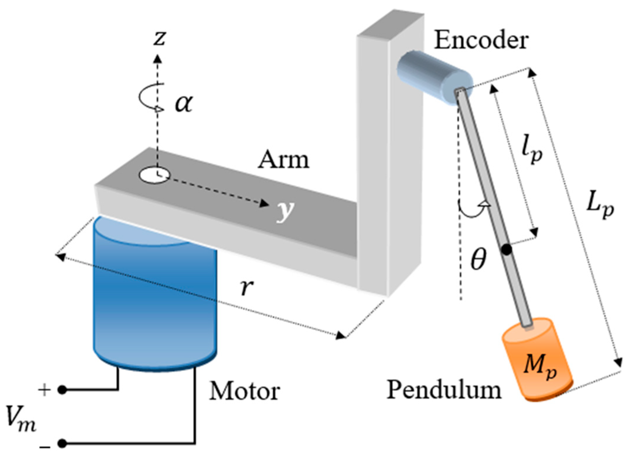
Figure 1. Schematic of the SLRIP system [22].
Machines 13 00939 g001
Figure 2. Block diagram of the baseline LQR law.
Machines 13 00939 g002
Figure 3. Waveform of the cubic HTF formulated for error normalization.
Machines 13 00939 g003
Figure 4. MF waveforms of (a) input variables, and (b) output variable.
Machines 13 00939 g004
Figure 5. Block diagram of the FLQR law.
Machines 13 00939 g005
Figure 6. Block diagram of the proposed SR-FLQR law.
Machines 13 00939 g006
Figure 7. Parameter selection process [21].
Machines 13 00939 g007
Figure 8. Quanser rotary pendulum platform used for HIL experiments [21].
Machines 13 00939 g008
Figure 9. Experiment A: Normal position regulation behavior of SLRIP.
Machines 13 00939 g009
Figure 10. Experiment B: Impulsive disturbance compensation behavior of SLRIP.
Machines 13 00939 g010
Figure 11. Experiment C: Step disturbance compensation behavior of SLRIP.
Machines 13 00939 g011
Figure 12. Experiment D: Sinusoidal disturbance attenuation behavior of SLRIP.
Machines 13 00939 g012
Figure 13. Experiment E: Model error rejection behavior of SLRIP.
Machines 13 00939 g013
Figure 14. Experiment A: Normal position regulation behavior of SLRIP.
Machines 13 00939 g014
Figure 15. Experiment B: Impulsive disturbance compensation behavior of SLRIP.
Machines 13 00939 g015
Figure 16. Experiment C: Step disturbance compensation behavior of SLRIP.
Machines 13 00939 g016
Figure 17. Experiment D: Sinusoidal disturbance attenuation behavior of SLRIP.
Machines 13 00939 g017
Figure 18. Experiment E: Model error rejection behavior of SLRIP.
Machines 13 00939 g018
Table 1. Model specifications of Quanser SLRIP [41].
ParameterDescriptionValueUnit
MpPendulum’s mass0.027kg
lpPivot to pendulum’s center distance0.153m
LpPendulum link length0.191M
rHorizontal arm length0.083M
MarmArm’s mass0.028Kg
gAcceleration due to gravity9.810m/s2
JeMoment about motor shaft1.23 × 10−4kgm2
JpMoment about pendulum1.10 × 10−4kgm2
RmMotor’s armature resistance3.30Ω
LmMotor’s armature inductance47.0mH
KtMotor torque coefficient0.028Nm
KmBack-EMF coefficient0.028V/(rad/s)
TmMaximum torque0.14Nm
Table 2. Fuzzy inference rule-base used for online control adjustment.
ε n / ε ˙ n NBNMNSZPSPMPB
NBNBNBNBNBNMNSZ
NMNBNBNBNMNSZPS
NSNBNBNMNSZPSPM
ZNBNMNSZPSPMPB
PSNMNSZPSPMPBPB
PMNSZPSPMPBPBPB
PBZPSPMPBPBPBPB
Table 3. Quantitative evaluation of experimental results.
ExperimentQPMControl Scheme
SymbolUnitLQRFLQRSR-FLQR
ARMSEθdeg.0.490.430.38
RMSEαdeg.14.6413.3810.81
MSVm V27.537.095.87
BRMSEθdeg.0.820.660.52
Mp,θdeg.2.872.582.15
Ts,θs.0.780.610.52
RMSEαdeg.13.749.828.42
MSVmV210.0610.197.52
VpV−11.94−10.05−8.99
CRMSEθdeg.0.960.680.45
RMSEαdeg.34.8126.9821.31
αoffdeg.−42.12−29.92−25.40
αp-pdeg.30.7833.8821.37
MSVm V227.7021.0117.98
DRMSEθdeg.0.510.470.38
RMSEαdeg.10.938.214.29
MSVm V213.2111.348.57
ERMSEθdeg.1.010.830.62
RMSEαdeg.16.8414.2211.18
MSVm V211.2912.4210.03
Table 4. Comparative analysis of SMC with SR-FLQR.
ExperimentQPMControl SchemeImprovement in SR-FLQR (%)
SymbolUnitSMC [7]SR-FLQR
ARMSEθdeg.0.400.385.0
RMSEαdeg.11.8510.818.8
MSVm V219.715.8770.2
BRMSEθdeg.0.610.5214.8
Mp,θdeg.2.202.152.3
Ts,θs.0.720.5227.8
RMSEαdeg.10.348.4218.6
MSVmV214.717.5248.9
VpV−16.02−8.9943.9
CRMSEθdeg.0.910.4550.5
RMSEαdeg.27.7021.3123.1
αoffdeg.−35.91−25.4029.3
MSVm V230.3317.9840.7
DRMSEθdeg.0.440.3813.6
RMSEαdeg.8.694.2950.6
MSVm V219.948.5757.0
ERMSEθdeg.1.060.6241.5
RMSEαdeg.12.4211.1810.0
MSVm V222.5410.0355.5
Disclaimer/Publisher’s Note: The statements, opinions and data contained in all publications are solely those of the individual author(s) and contributor(s) and not of MDPI and/or the editor(s). MDPI and/or the editor(s) disclaim responsibility for any injury to people or property resulting from any ideas, methods, instructions or products referred to in the content.