Fault Diagnosis in a 2 MW Wind Turbine Drive Train by Vibration Analysis: A Case Study

Abstract

This paper presents a vibration analysis method for detecting typical faults in gears of the drive train of a 2 MW wind turbine. The data were collected over a one-year period from an operating wind turbine with a gearbox composed of one planetary stage and two helical gear stages. Failures in two pairs of helical gears were identified: one involving pitting and wear in the gears connecting the intermediate-speed shaft to the low-speed shaft, and another one involving significant material detachment in the gears connecting the intermediate-speed shaft to the high-speed shaft. The continuous evaluation of time signals, frequency spectra, and amplitude modulations allowed the most sensitive sensors and frequencies for predicting surface damage on gear teeth in this type of turbine to be determined. A steady-state frequency analysis was performed, enabling the detection of the aforementioned surface faults. This approach is simpler compared with more complex transient-state techniques. By tracking vibration signals over time, the importance of analyzing gear mesh frequencies and their harmonics was highlighted. Additionally, it was found that the progression of gear damage was dependent on the power output of the wind turbine. As a result, the most appropriate ranges of power were identified, within which the evolution of the vibration measurement was associated with the damage evolution. Since many turbines currently in operation have similar designs and power output levels, the present findings can serve as a guideline for monitoring an extensive number of units.

1. Introduction

Growing interest in promoting energy sources that reduce the dependence on non-renewable sources and that have a lower environmental impact has driven the development of the wind energy industry over the past three decades [1]. Wind turbines have become particularly attractive given that their carbon emissions are 99% lower than those of most fossil fuels throughout their lifecycle [2]. By 2024, global wind energy capacity reached 906 GW, with significant contributions from China, Brazil, the USA, and Europe. Of this installed capacity, 70.6% corresponds to onshore turbines and 29.4% to offshore turbines [3]. Although studies indicate that larger turbines result in reduced carbon emissions per kilowatt-hour of generated electricity [4], 2 MW turbines, such as the models from Vestas, GAMESA, and Siemens (2.3 MW), remain prevalent.

The expansion of wind energy has driven the demand for reliable and efficient turbines; however, these systems are susceptible to failures such as torsional vibration, lateral bending, and longitudinal tower flexion due to the complex variable mechanical loads they endure. These loads impact the structural integrity of the blades and the nacelle, with issues in the drive train being the most critical within the turbine [1]. According to the National Renewable Energy Laboratory, the maintenance cost of a wind turbine is approximately $43 per kW per year [5]. The high cost of maintenance, the associated downtime, and the risk of catastrophic failures have focused researchers’ attention on predictive maintenance for drive trains in these types of turbines.

Monitoring techniques such as oil analysis, electrical signal analysis, and vibration analysis have been developed to detect faults in wind turbine drive trains; however, the most popular of them for rotating parts such as gearboxes and bearings is vibration analysis [6]. Primary faults that can be detected through vibration analysis in drive trains are those occurring in bearings and gears, which are the most critical components in power transmission. Vibration analysis for these types of elements can be performed through signal processing in the time domain, in the frequency domain, or through time–frequency analysis [7]. F. Castellani et al. [8] developed a fault detection algorithm for the drive train of wind turbines by processing statistical variables in the time domain using vibration measurements taken on the tower rather than from the gearbox. D. Siegle et al. [9] studied time-synchronous averaging with narrowband and residual methods for the parallel-stage gears and the ring gear of a wind turbine. Time-domain techniques are also complemented by research that develops dynamic models of certain drive-train components. P. Srikanth and A.S. Sekhar [10] proposed an 18-degree-of-freedom model of the rotor, gearbox, and generator of a 5 MW turbine, obtaining time-domain responses as a preliminary step for condition monitoring in this type of turbine, where signals are nonlinear and non-stationary. Additionally, C.V.H. Gayatri and A.S. Sekhar [11] developed a more robust 22-degree-of-freedom model specifically for the two helical stages of the gearbox, obtaining the system’s time-domain response.

Frequency analysis provides a better exploration of fault origins compared with time analysis, using classical methods such as Fast Fourier Transform for stationary signals [12]. For non-stationary signals, advanced methods, including, among others, the Wavelet Transform, Variational Mode Decomposition, and Local Mean Decomposition methods [13, 14, 15], have been developed and refined in recent years, which enable a more effective analysis of these signals. While these methods address many issues with non-stationary signals, wind turbine drive trains are complex systems subject to highly variable force ranges due to their dependence on wind speed and humidity. This variability can reduce the detection accuracy, often necessitating a specific analysis approach for each turbine type. Studies have therefore been conducted on wind turbines to obtain their unique signature [16] and to allow for damage detection by identifying amplitude changes at fault frequencies [8]. Various predictive approaches have also been proposed based on outputs from SCADA systems, as seen in studies by A.R. Nejad et al. [17] and Q. Zhong et al. [18], and as reviewed by Z. Liu and L. Zhang [7].

Although many vibration analysis techniques can be applied to wind turbines, detecting a fault in the power transmission system and monitoring its evolution over time may not be an easy task. This is because not all vibration sensors installed in a wind energy system are capable of capturing every fault and therefore cannot always track their development. Vibration monitoring systems in wind turbines measure vibrations within specific frequency ranges, which are limited by the sensitivity and sampling rate of each sensor. These parameters depend on both the sensor’s capabilities and its configured settings.

As a result, some sensors may not detect faults that occur at frequencies beyond their measurable range or outside their sensitivity threshold. In real-world applications where Supervisory Control and Data Acquisition (SCADA) systems are used, accelerometer data are stored in predefined frequency bands, where typical faults are expected to occur. However, the configuration of these frequency bands may not always be precise, which limits the accurate identification of faults.

Assessing the actual fault detection capability of accelerometers in wind turbines is challenging, as this would require inducing controlled and isolated faults to evaluate their impact on vibration measurements—a process that is not feasible in operational turbines. Given the limited information on this topic in the current literature, this work investigates the vibration signals of a 2 MW wind turbine, measured at various positions, and it compares these findings with inspection results that identified pitting and spalling on gears, as these are essential components in wind energy systems [19, 20]. The turbine examined is part of a 20-turbine wind farm with a total capacity of 40 MW. Although these turbines operate under transient conditions, it is possible to study anomalies at various stages of progression through steady-state analysis by appropriately selecting the monitoring parameters in the time and frequency domains, which, in turn, can significantly simplify the turbine condition assessment. The results identify which sensors are the most effective in detecting the studied faults and clarify the relationship between vibration measurements, operating conditions, and the failure progression for this type of turbine.

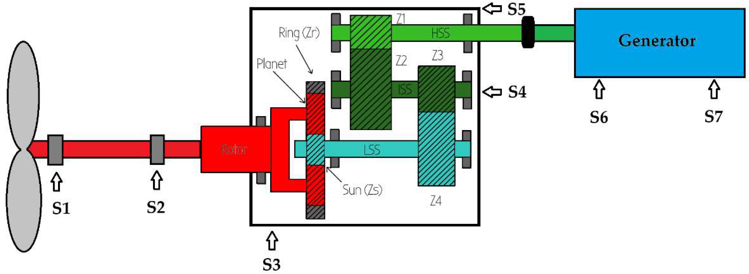
2. Description of the Turbine and Gearbox

Vibration signals were recorded from an operational 2 MW wind turbine. The turbine consists of the rotor, nacelle, and tower. The rotor includes fiberglass-reinforced plastic blades that convert the linear motion of the wind into rotational motion, with a rotor diameter of 90 m. The hub serves as the connection between the blades and the main shaft, transmitting wind force into the nacelle. Finally, the rotor nose extends outward from the blade–hub junction to direct airflow from the rotor front toward the nacelle vents and to minimize turbulence.

The gearbox, housed within the nacelle, adjusts the main shaft’s rotational speed to match the generator’s nominal speed (1500 rpm). The gearbox has multiple stages to handle high power and load requirements and to significantly increase the shaft’s rotational speed. In the first stage, the low-speed shaft (LSS), which is connected to the rotor that rotates at the blade speed, is coupled with the hollow shaft inside the gearbox via a planetary gear set. The rotor is coupled to the planet gears, while the hollow shaft is connected to the sun gear. After the rotor’s motion is transmitted to the hollow shaft, it is sequentially transferred to the intermediate-speed shaft (ISS) and, finally, to the high-speed shaft (HSS). These two last transmissions occur between parallel shafts via helical gears. The total transmission ratio is 112.8 for the turbine. Figure 1 shows a schematic representation of the analyzed wind turbine: Z1 is the number of teeth on the pinion of the HSS, Z2 is the number of teeth on the gear wheel of the ISS, Z3 is the number of the teeth on the pinion of the ISS, Z4 is the number of teeth on the gear wheel of the LSS, Zs is the number of teeth on the sun gear, and Zr is the number of teeth on the ring. The gears are manufactured from high-strength alloy steel that has been carburized, ground, and hardened to improve its durability under high-torque loads. All the gear components are mounted in a housing constructed from nodular cast iron.

In gear vibration analysis, an important frequency is the gear mesh frequency (GMF), defined as the product of the shaft rotation frequency and the number of gear teeth. This frequency represents the interaction frequency between pairs of teeth. Therefore, in this type of turbine, three gear mesh frequencies are of interest: GMF1, which is induced by the interaction between the planet gears and the sun gear; GMF2, which is induced by the interaction between the LSS gear and the ISS gear; and GMF3, which is induced by the interaction between the ISS gear and the HSS gear. The expressions to calculate the last two frequencies mentioned, which were analyzed in this work, are shown in Equations (1) and (2) as a function of the rotor frequency, f₀, and the number of teeth, Z, of the gears.

$$GMF2=Z4\left(f_0{\displaystyle \frac{Z_s+Z_r}{Z_s}}\right)$$

(1)

$$GMF3=Z2\left[{\displaystyle \frac{Z4}{Z3}}\left(f_0{\displaystyle \frac{Z_s+Z_r}{Z_s}}\right)\right]$$

(2)

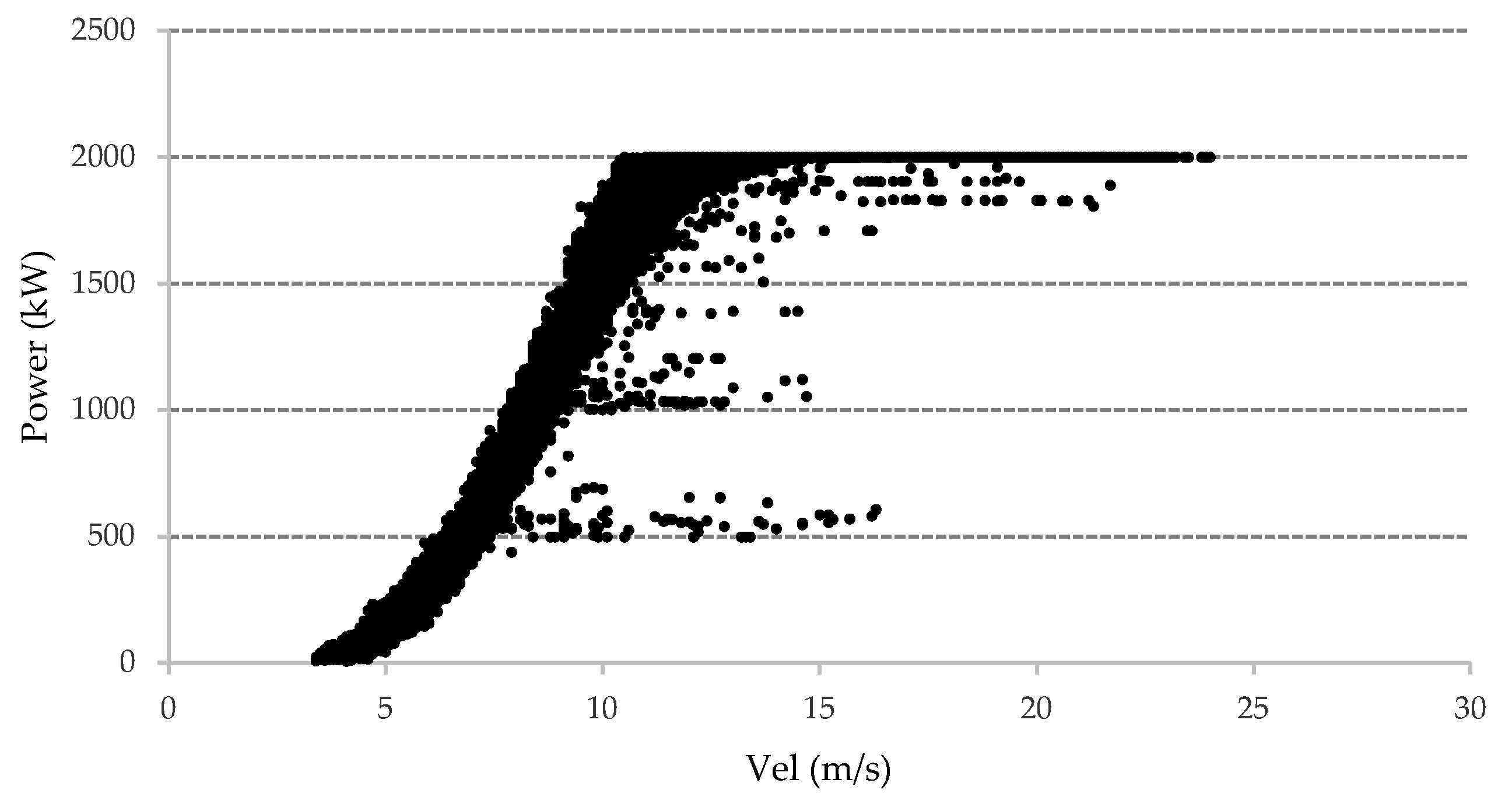
Operating Conditions

To ensure the proper operation of a wind turbine, effective control against wind fluctuations is essential to protect it from unacceptable maximum wind speeds. Regulating the rotational speed of wind turbines is straightforward, as explained below. When the wind speed reaches the cut-in speed (4 m/s), which is sufficient to release the brakes, the rotor begins to turn. At this point, the power output is low and gradually varies according to the wind speed. Through torque control of the generator, the rotor is regulated to reach its precise operational speed, or nominal speed, at which the turbine can function under standard conditions. When operating under optimal conditions—nominal speed and power—further increases in wind speed are undesirable. At this stage, regulation is achieved by adjusting the blade pitch angle, or the angle of attack of the wind on the blades. If the wind speed exceeds a certain threshold (cut-out speed, 25 m/s), the wind turbine brakes or disconnects, as the rotor’s structural integrity could be at risk. Figure 2 shows the characteristic curve of the turbine over a period of one year, with data taken every 10 min. Some points are observed that deviate from the ideal curve due to adjustments made in the machine according to the energy demand at the time.

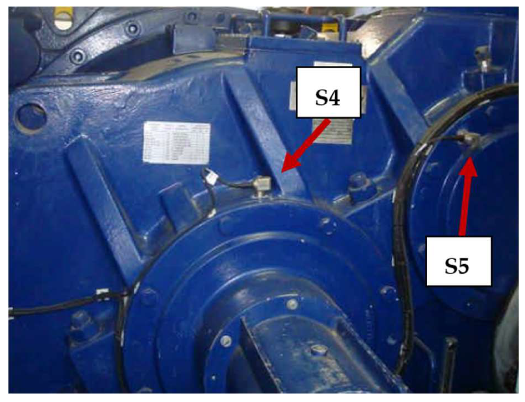
3. Vibration Monitoring System

The machines are equipped with a condition monitoring system that allows the reception of signals from seven industrial IEPE accelerometers located at different positions along the drive train. Vibration levels are expressed in acceleration units, and the signals can be saved in the time domain for later processing. The notation of the accelerometers and the nearest element to where they are located are shown in Figure 1 as follows: S1, front rotor bearing; S2, rear rotor bearing; S3, planetary transmission multiplier; S4, parallel transmission multiplier (vertical); S5, parallel transmission multiplier (axial); S6, front generator bearing; and S7, rear generator bearing. The actual location of two sensors can be seen in the photograph shown in Figure 3. The system enables remote monitoring of the wind farm. Changes detected in some components can be reported via a network (TCP/IP) to the wind-farm operator and the service provider. The signal from each sensor is analyzed using the signal acquisition system, which allows for the calculation and storage of up to 12 values per sensor. The system records acceleration values at predefined frequencies at which faults may occur in components such as shafts, blades, bearings, or gears. For the studied turbine, the recorded frequencies related to shaft failures are the shaft’s rotational frequency (1X) and its third harmonic (3X), which corresponds to the turbine’s blade-passing frequency (BPF) and which serves to detect blade faults. To detect bearing faults, the system records the ball spin frequency (BSF), the ball pass frequency on the inner race (BPFI) and its second harmonic (2XBPFI), the ball pass frequency on the outer race (BPFO) and its second harmonic (2XBPFO), as well as the fundamental train frequency (FTF). For faults associated with gears, the recorded frequencies include the previously described gear mesh frequencies (GMFs), along with certain harmonics, as follows: GMF1, 2XGMF1, 3XGMF1, 4XGMF1, 5XGMF1, GMF2, 2XGMF2, 3XGMF2, 4XGMF2, GMF3, 2XGMF3, 3XGMF3, and 4XGMF3.

The system is configured to store the amplitudes of up to 12 specific narrowband frequencies per sensor, based on the most probable damage that can be detected with that sensor. As an example, for sensor S6, the stored frequencies include BB, FTF, 1X, BPFO up to its third harmonic, 2XBSF, 2X(2XBSF), 3X(2XBSF), and BPFI up to its third harmonic. These frequencies are expected to be the main indicators of faults associated with the front bearing of the generator.

4. Methodology

This study analyzed the vibration data from an operational 2 MW wind turbine using its existing condition monitoring system. The turbine’s native configuration included seven accelerometers (S1–S7) at standard gearbox and bearing locations (Figure 1). Sensors S1, S2, and S3 had a sensitivity of 500 mV/g with a frequency range from 0.16 to 8000 Hz, while sensors S4, S5, S6, and S7 had a sensitivity of 100 mV/g with a frequency range from 0.5 to 8000 Hz. The sampling frequencies were 300 Hz for S1, 600 Hz for S2 and S3, 3000 Hz for S4, and 6000 Hz for S5 and S6. The time lengths of the recorded samples were 1.36 and 0.68 s for the measurements sampled at 3000 and 6000 Hz, respectively.

Vibration signals were processed through the turbine’s onboard system, which computed the following:

• Time-domain waveforms.
• Frequency spectra via Fast Fourier Transform (FFT).
• RMS amplitudes for 12 predefined narrowband frequencies per sensor (including GMFs and bearing-fault frequencies).

Given the system’s limitations and operational reality, steady-state analysis was prioritized. While wind turbines experience speed variations, the short-length data acquired and a validation check of the steady conditions carried out during the measurements allowed a reliable analysis through the following:

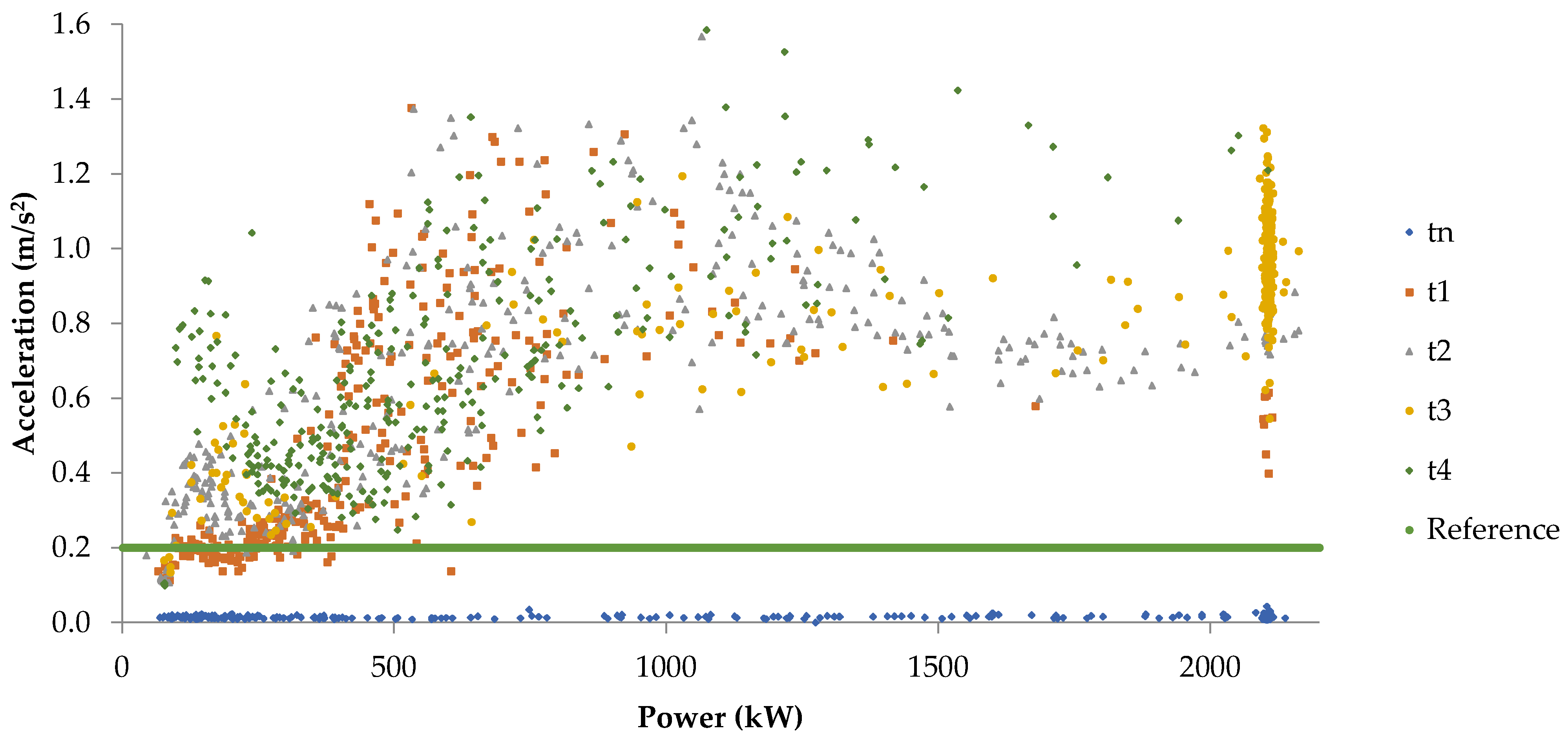
• Minimizing transient effects.
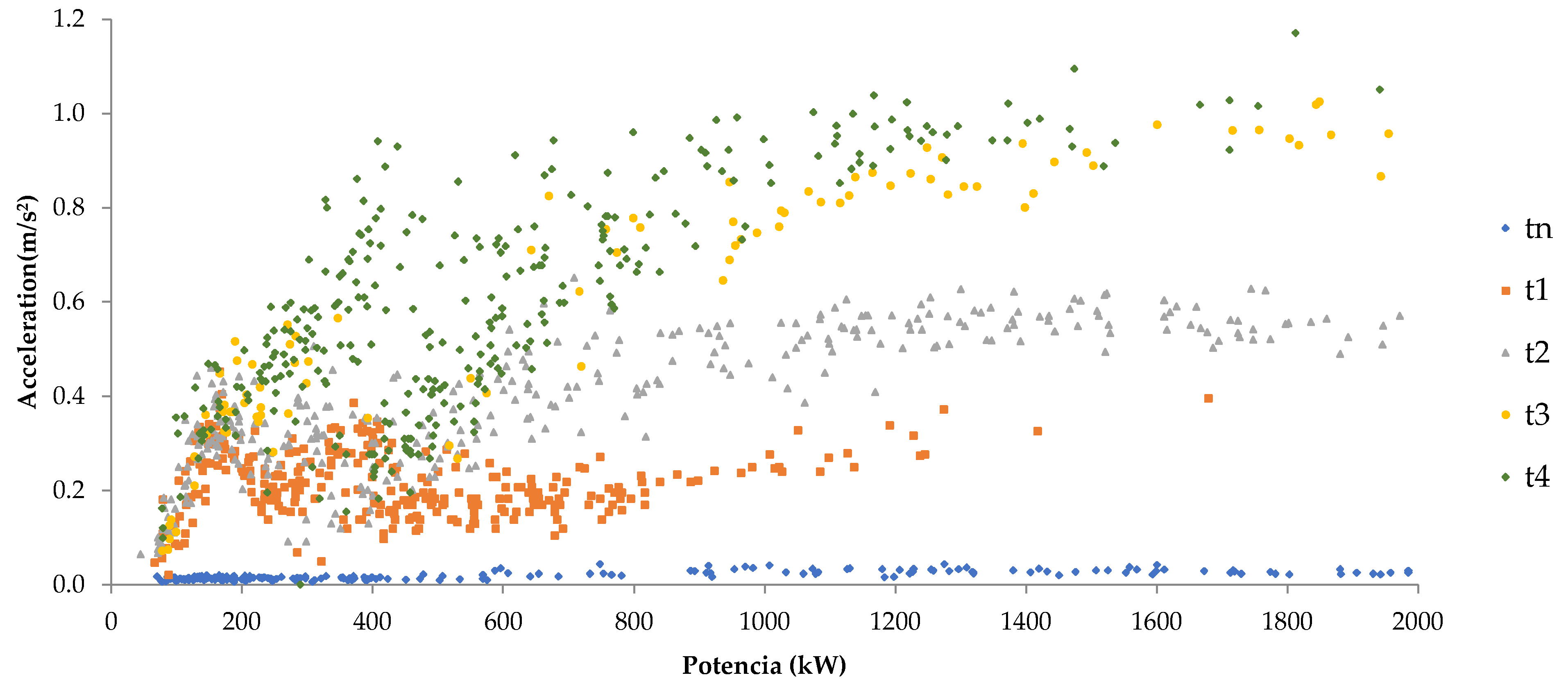
• Allowing a comparison of signals at similar power outputs.
• Focusing on higher harmonics (3XGMF/4XGMF), where fault progression was most evident.

Gear faults were first identified through vibration anomalies, then confirmed via endoscopic inspections during maintenance (Figure 4 and Figure 5). Data from a replaced gearbox and historical signatures of healthy turbines [16] served as baselines. Due to the proximity of the sensors to the studied faults, accelerometers S4, S5, and S6 were analyzed in more detail. The different frequency bands stored by the acquisition system were examined to identify where a significant increase occurred and in which band the damage progression could be observed. For those identified frequencies that showed a progressive increase in acceleration values, a regression model was proposed for each of the time intervals studied. This model was developed using an analysis of variance (ANOVA), and its statistical validity has been demonstrated for the operating ranges considered. Since power output appears to be a more direct indicator of drive-train loading than wind speed, we focused our comparative analysis of vibration spectra and amplitude levels on consistent power output ranges.

5. Results and Discussion

5.1. Data Acquisition and Processing

To study gear damage in the gearbox of the turbine, data from a 12-month period were analyzed. This period was segmented into three intervals of four months each to evaluate whether the targeted damage showed progression over time. In each interval, 300 data points were collected over at least five consecutive days. More specifically, four observation periods were defined and named consecutively: t1, for the initial observation period; t2, in the fourth month; t3, in the eighth month; and t4, in the twelfth month. For validation purposes, the data from an additional period, tn, located 9 months after the end of period t4 was also considered. These data correspond to a completely new gearbox that replaced the damaged one.

To investigate the damage associated with gear pairs mounted on the HSS and ISS, data from sensors S4, S5, and S6 were analyzed due to their proximity to the gears. Although sensor S6 is located on the generator, it was included in the analysis because of its position near the HSS.

The monitoring system installed in this equipment allows two types of data to be recorded: time signals of acceleration levels at different sampling frequencies, depending on the sensor; and amplitude levels of the predefined frequency bands of the turbine rotating speed (up to 12 per sensor), as mentioned before. The time-domain acceleration signals are digitized and processed using a digital signal processor, which enables the calculation of their frequency spectra and their storage in the monitoring system’s memory. To determine the amplitude levels of the frequencies of interest, the system computes the root mean square (RMS) value A_RMS of the frequency spectrum within a specified band, as expressed with Equation (3). The minimum frequency, f₁, and maximum frequency, f₂, are defined when the system is configured.

$$A_{RMS}=\sqrt{{\displaystyle \frac{1}{N}}{\sum }_{f_1-f_2}{A}^2}$$

(3)

Although wind turbine speed conditions are inherently variable, a transient analysis could make fault detection unnecessarily complex. One of the objectives of this work is to demonstrate that steady-state analysis can be effectively applied to such equipment for the detection of certain faults and yield good results. To achieve this, the monitoring system automatically verifies if a measurement has been taken during a range between the cut-in speed and the cut-out speed. The sampling rate and the time period are 6000 Hz and 0.68 s for sensors S6 and S5, and they are 3000 Hz and of 1.36 s for sensor S4. Nevertheless, the frequency plots used in the present study were double-checked to ensure that no distortions occurred in critical frequencies because of a possible speed variation during the measurement.

As shown in Figure 2, the output power vs. wind speed data closely align with the machine’s characteristic curve due to the power control system integrated into the equipment. However, certain power restrictions are evident, particularly at 500 kW and 1000 kW and within other ranges. These restrictions occur because even though the speed at certain moments could allow for a higher power output, the values are constrained by the existing energy demand conditions, as previously mentioned. Excluding cases that deviate from the theoretical operating curve, the output power can be considered a variable that is dependent on the speed. Therefore, to enable meaningful comparisons between spectra, it is necessary to analyze data collected under similar power conditions, as these will also correspond to similar wind speed values for the reasons explained above.

In order to assess the measurements against some reference levels, it was decided to use the results obtained in a previous study, where a large sample of healthy wind turbines of identical sizes and designs from the same wind farm was investigated to determine the average vibrational signatures of the drive-train components during normal operation [16]. The values recorded in that study correspond to averaged values for all the turbines in that wind farm at different frequencies of interest, making them useful as a comparative reference.

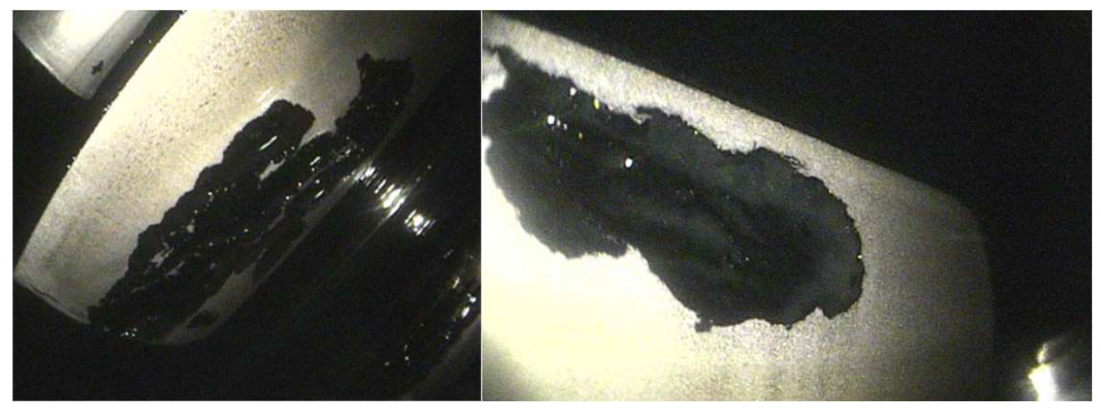
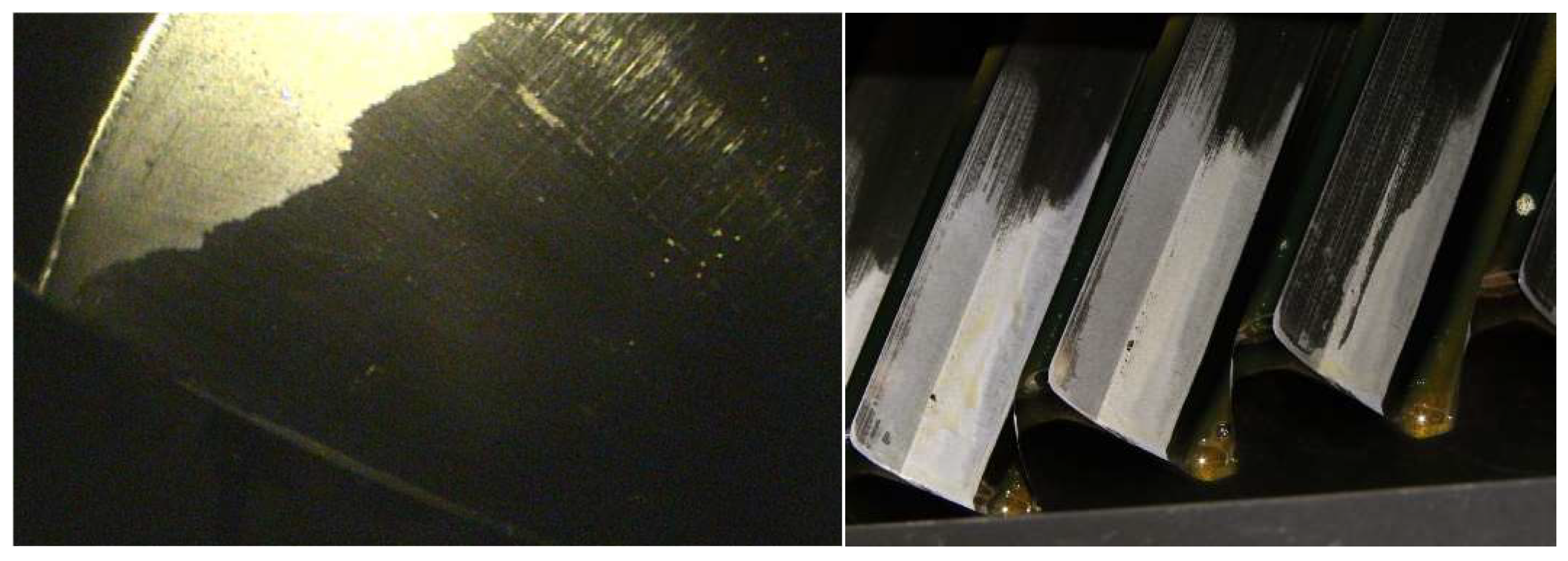
5.2. Pitting and Spalling

The internal inspection of the gearbox using an endoscope revealed damage in the gear pair coupled to the HSS, which consisted of pitting and spalling on the pinion teeth, as can be seen in the photographs shown in Figure 4. Pitting is a type of damage caused by surface fatigue resulting from the repeated pulsed loading of gear teeth during mesh engagement. It manifests as small, localized craters. This initial form of surface fatigue can progress to a more severe stage, known as spalling, where the damage leads to the detachment of material fragments from the surface. This type of damage is usually expected to manifest at the GMF3 gear mesh frequency or its harmonics. For detection purposes, these frequencies were examined using data from sensors S4, S5, and S6.

5.2.1. Sensor S4

It has to be noted that 1500 Hz is the maximum frequency that can be considered in the S4 spectrum given the sampling rate, according to the Nyquist theorem. Moreover, given the number of teeth, the GMF3 value for the turbine is 25 times the rotational frequency of the HSS. Therefore, for the vertically orientated S4 sensor, the monitoring system only records GMF3 and 2XGMF3 values as higher harmonics, such as 3XGMF3 or 4XGMF3, exceed 1500 Hz at many speeds.

The acceleration levels of the GMF3 frequency in S4 versus the turbine’s output power values are shown in Figure 6, which illustrates the values corresponding to the four observation periods with the damaged gearbox: t1, t2, t3, and t4, and the later observation period with the new gearbox. The graph shows that the values prior to the replacement are significantly higher compared with those measured with the new gearbox. Moreover, there is significant data dispersion, and no clear increasing trend over time is observed. Another important consideration is that the refence vibration signatures of the healthy wind turbines report a value of 0.8 m/s² for GMF3 at S4. So, it can be seen that, in spite of the advanced damage observed, all values across the different time intervals are found to be below that threshold. Given the fact that the acceleration values drop significantly after the gearbox replacement, this fact highlights that machine signatures and their reference levels, while a useful guide, might not be reliable as a unique indicator to detect damage.

For the 2XGMF3 frequency, a trend similar to that of GMF3 is observed, where the values before the gearbox replacement are higher than those with the new gearbox, as can be seen in Figure 7. In this case, the values starting from t3 within the power range of 1900 kW to 2000 kW clearly exceed the value of the reference signature, which is 0.2 m/s².

5.2.2. Sensor S5

The acceleration values for the GMF3 and 2XGMF3 frequencies were recorded for sensor S5. For GMF3, all values exceed the previously reported value of 1.25 m/s² from the vibration signature across all the studied times, as is shown in Figure 8. The lowest value, within the 1900 kW to 2100 kW power range, is 2 m/s², while the highest reaches 6 m/s². Although the amplitudes are significantly higher than those of the data recorded after the gearbox replacement, and the range between them is broad, no clear trend is observed for this frequency over time. For 2XGMF3, the behavior is similar, as can be seen in Figure 9. For this frequency, all values exceed the reference level of 0.2 m/s² taken from the reference signature, which ranges from 0.6 m/s² to 1.3 m/s², and are also well above the values reported for the new gearbox. However, no increasing trend over time is evident.

5.2.3. Sensor S6

The radial sensor S6 located at the front of the generator records acceleration values for the GMF3, 2XGMF3, and 3XGMF3 frequencies. However, for these frequencies, there is no evidence that the values recorded before the gearbox replacement are higher than those recorded after. The values for the 2 MW turbine range between 0.22 m/s² and 0.42 m/s². In this case, no reference amplitudes for healthy turbines using the signature information were available for these frequencies. Given that the reported values do not provide conclusive evidence of damage, this sensor may be irrelevant for analyzing this gear pair unless signatures for these frequencies are obtained. This behavior may occur because the sensor is located in the generator and is the farthest from the fault zone among the three analyzed sensors.

5.2.4. Comparison Between Sensors S4 and S5

When analyzing the 2XGMF3 frequency values, it is observed that relying solely on the signature values would suggest that sensor S4 begins to indicate damage only from t3 onward (Figure 7), despite the damage being expected to be present from t1. In this sense, these acceleration levels would provide a delayed warning for a fault that is already significantly advanced.

In contrast, sensor S5 shows high values above the reference threshold from t1 onward. Additionally, it can be observed in Figure 8 and Figure 9 that the values recorded by sensor S5 for the fault frequencies associated with this gear pair are higher than those from sensor S4. This may indicate that in this case, the development of pitting and material detachment had a greater impact on the axial forces than on the radial forces. This is plausible given the characteristics of helical gears, which transmit tangential, radial, and axial forces. Therefore, the fault will manifest more prominently in one direction or another depending on the location and propagation direction of the damage within the gear, as well as on the severity of the fault.

Based on the results presented for sensors S4 and S5, it is observed that although GMF3 and 2XGMF3 exhibit values that are higher across all times than both the reference values from vibration signatures and the values recorded for the new gearbox, no increasing trend is evident. This could indicate either that the damage was already well developed during the first period of time, t1, or that progression occurred but is only reflected in higher harmonics, such as 3XGMF3 or 4XGMF3. Therefore, it is recommended for this application to expand the sampling range for S4 and to store data for the 3XGMF3 and 4XGMF3 frequencies.

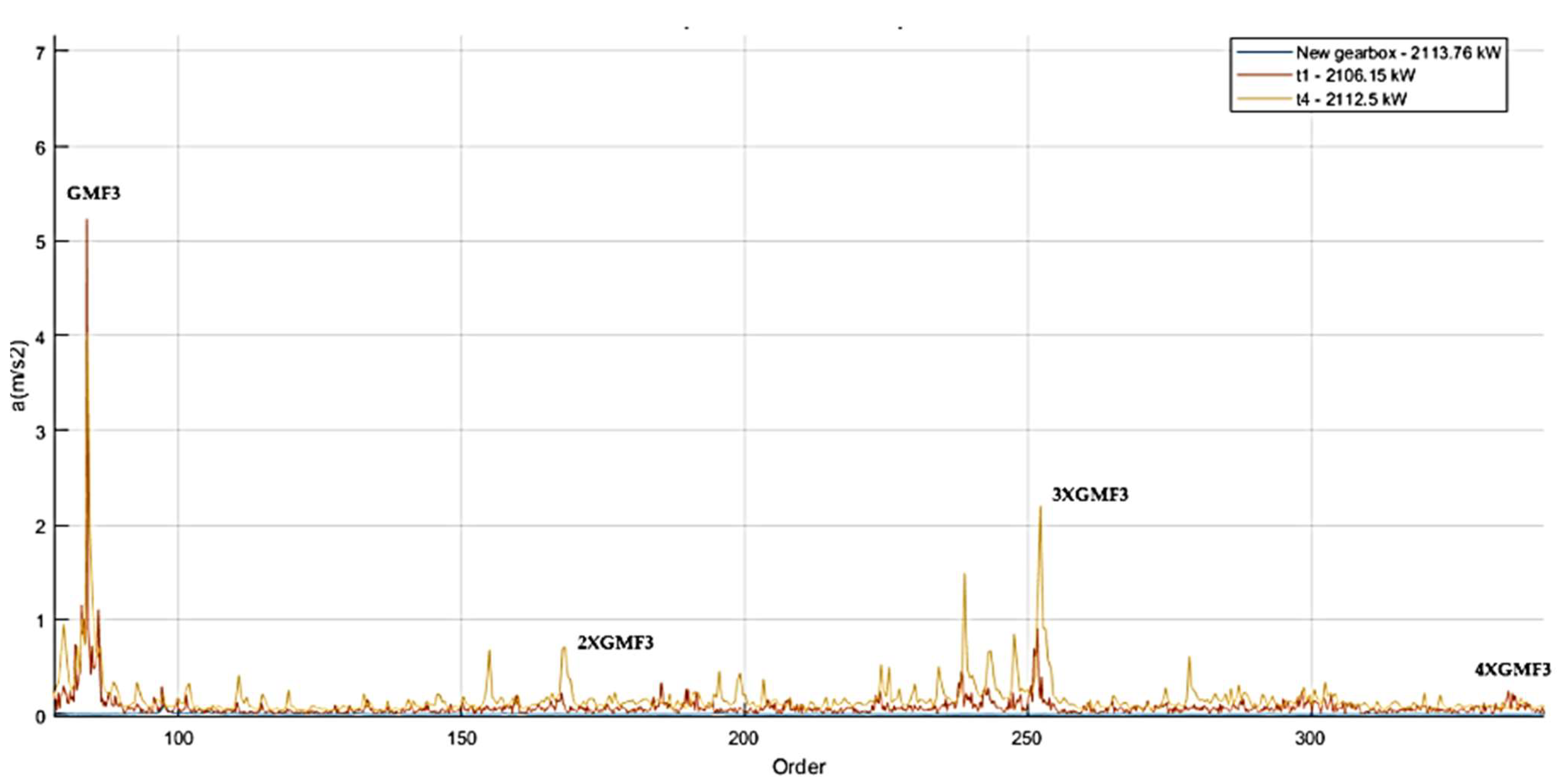
5.2.5. Spectra Comparison

Figure 10 shows three spectra corresponding to measurements from the axial sensor S5 at the start of monitoring during t1 and t4 as well as a spectrum from the newly installed gearbox. These spectra were taken when the turbine was operating at similar rotating speeds and power outputs of approximately 2100 MW. The spectra are presented in the order domain for better visualization, where an order of 1 corresponds to the rotational speed of the ISS.

The spectra in Figure 10 show vibration values for the gear mesh frequencies of the gear pair transmitting motion between the HSS and the ISS. Specifically, they show GMF3, 2XGMF3, 3XGMF3, and 4XGMF3, which correspond to orders 84, 168, 252, and 336, respectively. It can be observed that all acceleration values for these frequencies are above those of the new gearbox; however, there is a decrease in GMF3 between t1 and t4, making it unsuitable for monitoring damage evolution using this frequency.

In contrast, for 2XGMF3 and 3XGMF3, there is an increase in the vibratory signal over time, while for 4XGMF3, the signal decreases. Therefore, for these turbines, it is recommended to record 3XGMF3 results from the axial sensor to verify whether this type of damage could be monitored through this frequency.

5.3. Pitting and Wear

Upon inspection, pitting and wear were found on the pinion teeth of the gear pair connecting the ISS to the LSS., as shown in Figure 5. The frequencies of interest for detecting these faults are GMF2 and its multiples. Data recorded by sensors S4 and S5 were analyzed in this case. In addition, sensor S6 was also checked for validation purposes. The coexistence of pitting and wear in the ISS-LSS gear pair suggests a multi-stage failure process: initial pitting from contact fatigue (under adequate lubrication), followed by wear accelerated by micro-pitting-induced surface roughness, and transient lubrication breakdowns at high loads. This is consistent with the harmonic-specific vibration trends observed in S5 (Figure 11, Figure 12, Figure 13 and Figure 14) as will be shown.

5.3.1. Sensor S4

From sensor S4, the acceleration values of the GMF2 frequency and its second harmonic were analyzed. The values for the GMF2 frequency show no trend across the different time periods. The values are low both before and after the gearbox replacement, with the highest value being 0.07 m/s². While the signature value is 0.05 m/s², no increase is observed for power ranges near 2000 kW. The behavior at the 2XGMF2 frequency is similar, as there is no pattern in the data nor any evidence of a decrease after the gearbox replacement. The values for this frequency are also quite low, with the highest being 0.042 m/s². In this regard, these two frequencies do not represent an indicator for this type of gear failure.

5.3.2. Sensor S5

From the axial sensor S5, acceleration values were recorded for the GMF2, 2XGMF2, 3XGMF2, and 4XGMF2 frequencies. The GMF2 values are higher than the signature value of 0.05 m/s² across all times and are also greater than those recorded after the gearbox replacement. However, no increasing trend over time is observed. A similar behavior is noted for the 2XGMF2 frequency, where the values prior to the gearbox replacement exceed both the signature value of 0.2 m/s² and the post-replacement values, yet no clear progression over the studied times is evident.

The acceleration data recorded at the 3XGMF2 frequency by S5 are presented in Figure 11. It is evident that the values before the gearbox replacement are higher across all times compared with those recorded after the replacement. Additionally, an increasing trend is observed over the four studied time intervals, particularly for power levels between 1000 kW and 2000 kW. In this range, all values across all the studied times exceed the signature value of 0.1 m/s², with the minimum value being 0.24 m/s² in t1.

Since differentiated acceleration values by time intervals are evident for this frequency, the corresponding regressions were estimated for each period of time to analyze the relationship between output power and the measured acceleration levels and to understand how damage progresses at a given power range. In this context, the model inputs are power and time intervals, and the output is the acceleration measured at the given frequency. An analysis of variance (ANOVA) was conducted to identify the significant variables and interactions, ensuring that the model adequately describes the acceleration behavior for each time interval studied. Since it is more appropriate to use a separate regression model for each time interval, the significant variables were found to be power or exponential terms of power.

In this case, the model that best predicts the acceleration response is a sixth-degree polynomial equation, as the terms P, P², P³, P⁴, P⁵, and P⁶ were found to be statistically significant in every time interval, with p-values below 0.05.

To assess the relative dispersion of the data with respect to the mean, the coefficient of variation (CV) was calculated as a percentage according to Equation (4), where σ is the standard deviation of the data, and µ is the mean of the data. Given that the standard deviation is 0.1019 and the mean is 0.5204, the CV is 19.6%.

$$CV(\%)=\left({\displaystyle \frac{\sigma }{\mu }}\right)\times 100$$

(4)

For a regression model, a low CV is desirable, as it indicates good precision in the predictions, with residuals not being widely dispersed. Although 19.6% is not extremely low, this value is not considered alarming. This is further supported by the coefficient of determination (R²) and the adjusted R², which are 0.8904 and 0.8830, respectively. These are high values and show minimal difference between them.

Another parameter used to validate statistical models is the Adeq Precision, which evaluates how well the model can distinguish the “signal” from the “noise”. This is assessed through the signal-to-noise ratio, where a value greater than 4 is considered desirable. In this case, the value is 65.38, confirming that the model is suitable for predicting acceleration at this frequency within the studied operating range.

Figure 12 illustrates these regression models, and the equations for each time interval are shown in Equations (5)–(8), where a₁, a₂, a₃, and a₄ represent the vibration estimation in $m{s}^{-2}$ for the time periods t1, t2, t3, and t4, respectively, and P is the power in kW.

$$a_1=-6.81\times {10}^{-2}+3.55\times {10}^{-3}P-1.40\times {10}^{-5}{P}^2+2.23\times {10}^{-8}{P}^3-1.75\times {10}^{-11}{P}^4+6.57\times {10}^{-15}{P}^5-9.45\times {10}^{-19}{P}^6$$

(5)

$$a_2=8.68\times {10}^{-3}+3.05\times {10}^{-3}P-1.10\times {10}^{-5}{P}^2+1.96\times {10}^{-8}{P}^3-1.63\times {10}^{-11}{P}^4+6.37\times {10}^{-15}{P}^5-9.45\times {10}^{-19}{P}^6$$

(6)

$$a_3=-2.22\times {10}^{-1}+5.45\times {10}^{-3}P-1.70\times {10}^{-5}{P}^2+2.52\times {10}^{-8}{P}^3-1.89\times {10}^{-11}{P}^4+6.82\times {10}^{-15}{P}^5-9.45\times {10}^{-19}{P}^6$$

(7)

$$a_4=1.52\times {10}^{-2}+3.81\times {10}^{-3}P-1.30\times {10}^{-5}{P}^2+2.15\times {10}^{-8}{P}^3-1.73\times {10}^{-11}{P}^4+6.58\times {10}^{-15}{P}^5-9.45\times {10}^{-19}{P}^6$$

(8)

In Figure 12, it can be observed that the measured acceleration values in each time interval increase as power rises, as expected. However, analyzing the behavior of acceleration values for a given power reveals an increase over time within the range from 1000 kW to 2000 kW. For power levels below 1000 kW, there is no clear evidence of damage progression associated with an increase in acceleration, particularly between t3 and t4. At power levels below 250 kW, the acceleration values are even more scattered, and no damage progression can be observed in any of the times. Figure 5 and Figure 11 show the results for gear frequencies and their multiples for two different gear pairs: the one connecting the HSS to the ISS and the one connecting the ISS to the LSS. Since both figures indicate that for power levels below 1000 kW, it is not possible to detect damage across all the time intervals, it is recommended that wear-damage monitoring for this type of turbine be performed at power levels exceeding 1000 kW.

In the range between 1500 kW and 2000 kW, for the frequency 3XGMF2, it is observed that the acceleration levels grow progressively with time for all the power levels. Given that the inspection revealed evidence of wear and pitting, it can be deduced that the measured acceleration changes at this frequency are related to the progression of this wear. Figure 13 shows the evolution of acceleration at the 3XGMF2 frequency over the analyzed time period at the nominal power of 2000 kW. By the 12th month of analysis, the observed damage at the end of the time period was significantly large. At the reference value, where no wear is present, an acceleration of 0.1 m/s² was recorded. The figure illustrates the evolution of the acceleration level associated with wear; however, due to the nonlinearity of the process caused by load variations, a direct relationship between acceleration and wear cannot be established. Nevertheless, the figure serves as a reference for the evolution of acceleration levels linked to the increase in gear wear.

Acceleration values measured by sensor S5 at the 4XGMF2 frequency also show wear progression over time, although there are no clear differences between t3 and t4. Similarly to the approach used for the 3XGMF2 frequency, a relationship could be established between the acceleration and the analyzed time for a given power level. This would provide an additional indicator for estimating the evolution of the acceleration from another sensor associated with damage to the gear.

5.3.3. Sensor S6

For sensor S6, values for the GMF2 frequency or its harmonics were not recorded. However, an analysis of the spectra available from this sensor during the studied time periods revealed the presence of peaks corresponding to GMF2, 2XGMF2, 3XGMF2, and 4XGMF2. This finding must be approached with caution as, for this wind turbine, the GMF2 frequency coincides with the ball pass frequency of the outer race (BPFO) of a generator bearing. A demodulation analysis was performed, revealing that frequencies between 2000 and 2500 Hz demodulate to the BPFO frequency. While the BPFO of the generator’s front bearing in this case matches the GMF2 gear mesh frequency, it is more reasonable to attribute this demodulation to a bearing fault rather than to a gear frequency. Demodulations caused by gear faults are typically observed at the shaft rotation frequency. Therefore, it is likely that the signal captured by S6 corresponds to an anomaly in the generator’s front bearing rather than a failure in the gear pair.

5.3.4. Spectra Comparison

Figure 14 shows the gear mesh frequency of the gear pair connecting the ISS to the LSS and its first four harmonics: GMF2, 2XGMF2, 3XGMF2, and 4XGMF2, which correspond to orders 16, 32, 48, and 64, respectively. It can be observed that for GMF2 and 2XGMF2, the values at t1 and t4 are higher than those for the new gearbox. However, no increase is observed in the value at t4 compared with that at t1; in fact, for 2XGMF2, the value is lower, reflecting the previously mentioned observation that these frequencies do not allow for the monitoring of the progression of surface damage.

For 3XGMF2 and 4XGMF2, an increase in acceleration values is observed at t4 compared with at t1, with values higher than those recorded for the new gearbox. This confirms the importance of monitoring these two harmonics for tracking this type of damage.

5.4. Sensor Data Relationships and Optimization Implications

5.4.1. Multi-Sensor Correlation Analysis

Our study compared vibration signals from axial (S5), vertical (S4), and radial (S6) sensors to assess their sensitivity to gear faults. As a summary:

• Axial sensor S5 showed higher sensitivity to gear mesh frequencies (GMF3, 3XGMF2) and earlier fault detection (Figure 7, Figure 8, Figure 9, Figure 11 and Figure 12), which is likely due to helical-gear axial force transmission.
• Vertical sensor S4 provided complementary data but with lower amplitude signals (Figure 5 and Figure 6), suggesting that radial forces were less affected by the studied faults.

This contrast underscores the importance of multi-directional sensor placement to capture fault signatures comprehensively.

5.4.2. Fault-Specific Sensor Efficacy

• For HSS-ISS gear-pair damage (pitting/spalling), S5 (axial) outperformed S4 (vertical) in detecting 2XGMF3 and 3XGMF3 harmonics.
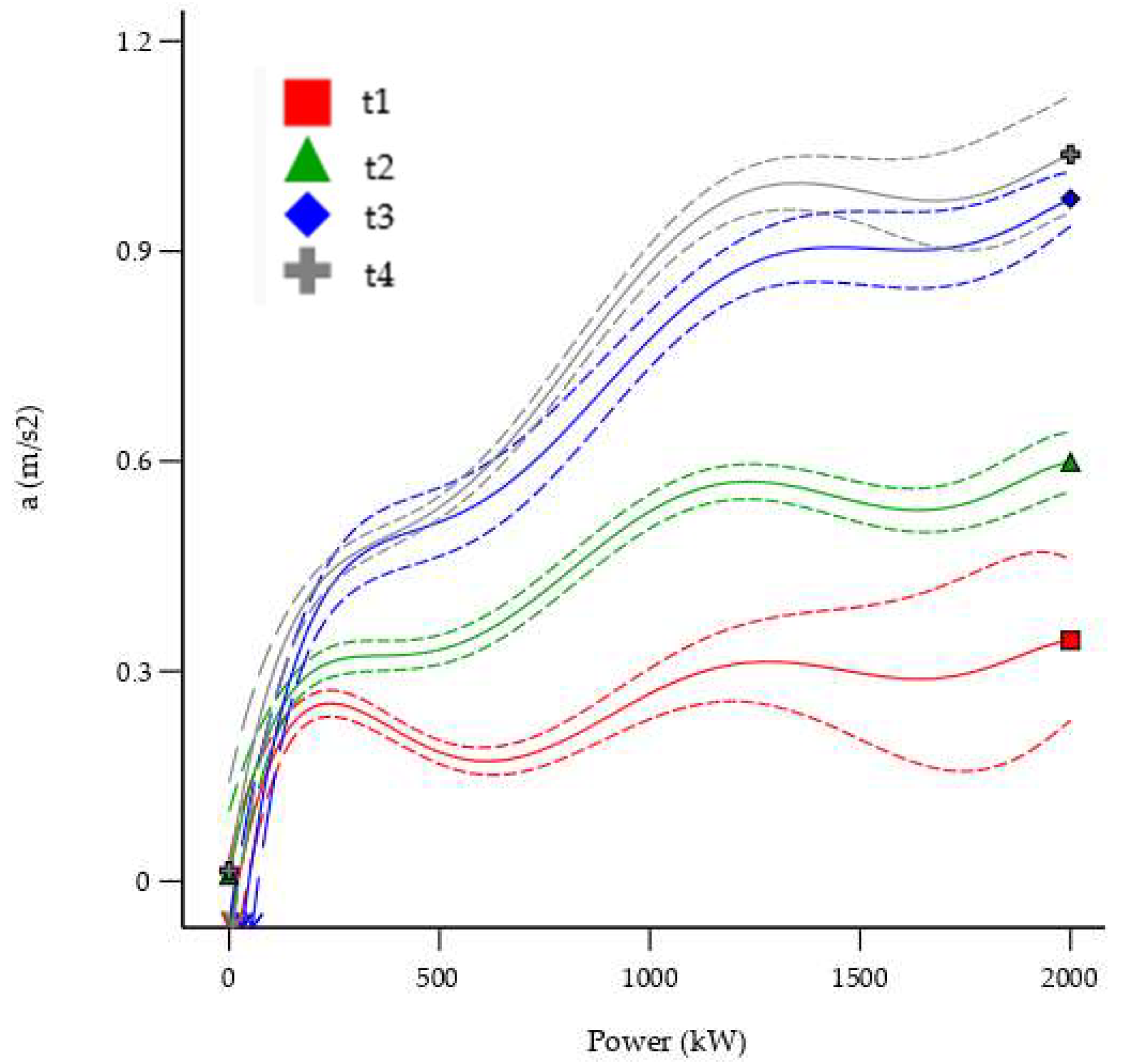
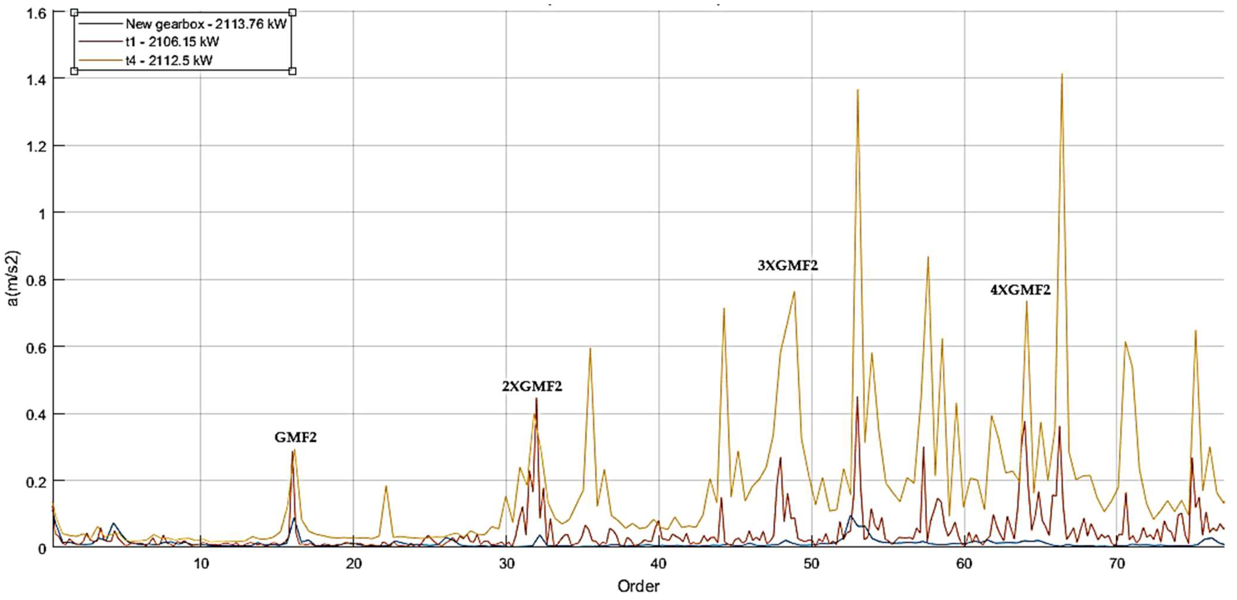
• For ISS-LSS gear wear, S5’s 3XGMF2 and 4XGMF2 harmonics exhibited clear progression trends (Figure 11), while S4’s GMF2/2XGMF2 data were inconclusive.
• Sensor S6 (generator-bearing) was less relevant for gear faults but highlighted risks of frequency aliasing (e.g., GMF2 overlapping with BPFO).

5.4.3. Implications for Sensor Optimization:

• Axial sensors are critical for helical-gear fault detection, as they capture axial load variations from tooth wear/pitting.
• Higher harmonics (3XGMF, 4XGMF) should be prioritized in monitoring systems, as they reveal damage progression better than fundamental GMFs (Figure 9 and Figure 14).
• Sensor placement should avoid spectral overlaps (e.g., gear and bearing frequencies) to reduce false alarms.

6. Conclusions

This study demonstrates that steady-state vibration analysis can effectively detect and monitor gear surface damage (pitting, spalling, and wear) in the examined 2 MW wind turbine gearbox under typical operating conditions. While transient methods may offer advantages for certain fault types or extreme operational scenarios, our results show that steady-state approaches provide a reliable and practical alternative for monitoring progressive gear wear (1) when the analysis focuses on higher gear mesh harmonics (3XGMF/4XGMF), and (2) when measurements are taken at power outputs above 1000 kW. The axial-sensor position proved particularly valuable for helical-gear monitoring, outperforming other radial/vertical sensors in sensitivity in detecting developing faults. These findings suggest that for turbines with similar designs and operating profiles, condition monitoring systems could benefit from prioritizing axial-sensor data and from incorporating higher harmonic analysis. However, we recommend complementary transient analysis when investigating incipient faults or when operating outside normal parameters. Future work should explore the boundaries of steady-state methods across different turbine classes and fault types.

References

1. Machado, M.R.; Dutkiewicz, M. Wind turbine vibration management: An integrated analysis of existing solutions, products, and Open-source developments. Energy Rep. 2024, 11, 3756–3791. [Google Scholar] [CrossRef]
2. Orsted. What Is the Carbon Footprint of Offshore Wind? 2022. Available online: https://orsted.com/en/what-we-do/insights/the-fact-file/what-is-the-carbon-footprint-of-offshore-wind (accessed on 1 February 2025).
3. Lee, J.; Zhao, F. Global Wind Report 2024. 2024. Available online: https://img.saurenergy.com/2024/05/gwr-2024_digital-version_final-1-compressed.pdf (accessed on 27 November 2024).
4. Smoucha, E.A.; Fitzpatrick, K. Life Cycle Analysis of the Embodied Carbon Emissions from 14 Wind Turbines with Rated Powers between 50 Kw and 3.4 Mw. J. Fundam. Renew. Energy Appl. 2016, 6, 1000211. [Google Scholar] [CrossRef]
5. Stehly, T.; Duffy, P. 2020 Cost of Wind Energy Review. 2020. Available online: www.nrel.gov/publications (accessed on 13 May 2025).
6. Teng, W.; Ding, X.; Tang, S.; Xu, J.; Shi, B.; Liu, Y. Vibration analysis for fault detection of wind turbine drivetrains—A comprehensive investigation. Sensors 2021, 21, 1686. [Google Scholar] [CrossRef] [PubMed]
7. Liu, Z.; Zhang, L. A review of failure modes, condition monitoring and fault diagnosis methods for large-scale wind turbine bearings. Measurement 2020, 149, 107002. [Google Scholar] [CrossRef]
8. Castellani, F.; Garibaldi, L.; Daga, A.P.; Astolfi, D.; Natili, F. Diagnosis of faulty wind turbine bearings using tower vibration measurements. Energies 2020, 13, 1474. [Google Scholar] [CrossRef]
9. Siegel, D.; Zhao, W.; Lapira, E.; Abuali, M.; Lee, J. A comparative study on vibration-based condition monitoring algorithms for wind turbine drive trains. Wind Energy 2014, 17, 695–714. [Google Scholar] [CrossRef]
10. Srikanth, P.; Sekhar, A.S. Dynamic analysis of wind turbine drive train subjected to nonstationary wind load excitation. Proc. Inst. Mech. Eng. C J. Mech. Eng. Sci. 2015, 229, 429–446. [Google Scholar] [CrossRef]
11. Gayatri, C.V.H.; Sekhar, A.S. Dynamic analysis and characterization of two stage epicyclic gear box in wind turbine drive train. AIP Conf. Proc. 2018, 2044, 020018. [Google Scholar] [CrossRef]
12. Jian, T.; Cao, J.; Liu, W.; Xu, G.; Zhong, J. A novel wind turbine fault diagnosis method based on compressive sensing and lightweight SqueezeNet model. Expert Syst. Appl. 2025, 260, 125440. [Google Scholar] [CrossRef]
13. Wei, H.; Zhang, Q.; Shang, M.; Gu, Y. Extreme learning Machine-based classifier for fault diagnosis of rotating Machinery using a residual network and continuous wavelet transform. Measurement 2021, 183, 109864. [Google Scholar] [CrossRef]
14. Dibaj, A.; Ettefagh, M.M.; Hassannejad, R.; Ehghaghi, M.B. A hybrid fine-tuned VMD and CNN scheme for untrained compound fault diagnosis of rotating machinery with unequal-severity faults. Expert Syst. Appl. 2021, 167, 114094. [Google Scholar] [CrossRef]
15. Yang, J.; Delpha, C. An incipient fault diagnosis methodology using local Mahalanobis distance: Fault isolation and fault severity estimation. Signal Process. 2022, 200, 108657. [Google Scholar] [CrossRef]
16. Escaler, X.; Mebarki, T. Full-scale wind turbine vibration signature analysis. Machines 2018, 6, 63. [Google Scholar] [CrossRef]
17. Nejad, A.R.; Odgaard, P.F.; Gao, Z.; Moan, T. A prognostic method for fault detection in wind turbine drivetrains. Eng. Fail. Anal. 2014, 42, 324–336. [Google Scholar] [CrossRef]
18. Zhong, Q.; Liu, S.; Liu, C.; Liu, W.; Liu, S.; Zhao, Y.; Wu, Y. Fault Diagnosis of Wind Turbine Gearboxes Based on Multisource Signal Fusion. IEEE Trans. Instrum. Meas. 2025, 74, 3526413. [Google Scholar] [CrossRef]
19. Wu, J.; Wei, P.; Zhu, C.; Zhang, P.; Liu, H. Development and application of high strength gears. Int. J. Adv. Manuf. Technol. 2024, 132, 3123–3148. [Google Scholar] [CrossRef]
20. Bußkamp, P.; Jacobs, G.; Röder, J. Multiobjective wind turbine gearbox design optimization to reduce component damage risk during grid faults. Forsch. Ingenieurwes. 2025, 89, 48. [Google Scholar] [CrossRef]
Figure 1. Gearbox diagram and sensor locations (S) in the analyzed turbine. Zi indicates the number of teeth for each gear shown.
Machines 13 00434 g001
Figure 2. Power output vs. wind speed curve for the turbine during a year.
Machines 13 00434 g002
Figure 3. Photograph showing the location of the vertical accelerometer (S4) and axial accelerometer (S5) on the gearbox near the ISS and HSS, viewed from the generator.
Machines 13 00434 g003
Figure 4. Pitting and spalling on the pinion gear mounted on the HSS.
Machines 13 00434 g004
Figure 5. Pitting (left) and wear (right) on the pinion gear mounted on the ISS.
Machines 13 00434 g005
Figure 6. Acceleration amplitudes of the GMF3 frequency versus power output in sensor S4 for the different time intervals: t1, for the initial observation period; t2, in the fourth month; t3, in the eighth month; t4, in the twelfth month; and tn, for the new gearbox replaced 9 months after the end of the t4 period.
Machines 13 00434 g006
Figure 7. Acceleration amplitudes of the 2XGMF3 frequency versus power output in sensor S4 for the different time intervals: t1, for the initial observation period; t2, in the fourth month; t3, in the eighth month; t4, in the twelfth month; and tn, for the new gearbox replaced 9 months after the end of the t4 period. The horizontal green line is the reference value for this frequency.
Machines 13 00434 g007
Figure 8. Acceleration amplitudes of the GMF3 frequency versus power output in sensor S5 for the different time intervals: t1, for the initial observation period; t2, in the fourth month; t3, in the eighth month; t4, in the twelfth month; and tn, for the new gearbox replaced 9 months after the end of the t4 period.
Machines 13 00434 g008
Figure 9. Acceleration amplitudes of the 2XGMF3 frequency versus power output in sensor S5 for the different time intervals: t1, for the initial observation period; t2, in the fourth month; t3, in the eighth month; t4, in the twelfth month; and tn, for the new gearbox replaced 9 months after the end of the t4 period. The horizontal green line is the reference value for this frequency.
Machines 13 00434 g009
Figure 10. Zoom frequency spectra in the order domain to visualize acceleration signals from the axial sensor S5 at the GMF3, 2XGMF3, 3XGMF3, and 4XGMF3 frequencies for measurements taken during three different periods of time: t1, for the initial observation period; t4, in the twelfth month; and for the new gearbox replaced 9 months after the end of the t4 period.
Machines 13 00434 g010
Figure 11. Acceleration amplitudes of the 3XGMF2 frequency versus power output in sensor S5 for the different time intervals: t1, for the initial observation period; t2, in the fourth month; t3, in the eighth month; t4, in the twelfth month; and tn, for the new gearbox replaced 9 months after the end of the t4 period.
Machines 13 00434 g011
Figure 12. Regression models of the 3XGMF2 frequency acceleration amplitudes in sensor S5 as a function of output power for each period of time: t1, for the initial observation period; t2, in the fourth month; t3, in the eighth month; t4, in the twelfth month. The dashed lines represent the confidence interval for each regression model.
Machines 13 00434 g012
Figure 13. Acceleration amplitudes of the 3XGMF2 frequency in sensor S5 as a function of time for an output power of 2000 kW.
Machines 13 00434 g013
Figure 14. Frequency spectra in the order domain of sensor S5 with an indication of the frequencies GMF2, 2XGMF2, 3XGMF2, and 4XGMF2 for three different periods of time: t1, for the initial observation period; t4, in the twelfth month; and for the new gearbox replaced 9 months after the end of the t4 period.
Machines 13 00434 g014
Disclaimer/Publisher’s Note: The statements, opinions and data contained in all publications are solely those of the individual author(s) and contributor(s) and not of MDPI and/or the editor(s). MDPI and/or the editor(s) disclaim responsibility for any injury to people or property resulting from any ideas, methods, instructions or products referred to in the content.